Acoustics Field and Active Structural Acoustic Control Modeling in ANSYS

M. S. Khan, C. Cai and K. C. Hung Institute of High Performance Computing

89-C Science Park Drive #02-11/12, The Rutherford Singapore Science Park 1, Singapore 118261

Abstract: This article attempts to examine acoustic finite element analysis coupled with structure, and provides the necessary information to apply ANSYS for a wide class of structural acoustics problem. First part of this article describes the acoustic field and hence the uses of acoustic point sources in ANSYS. Results are explained and compared with that of analytical solution. And second part deals with the active control of structural acoustic problems. Results are presented for global cancellation of a primary monopole's sound field by the use of multiple piezoelectric elements bonded to the surface of the elastic structure to provide control forces.

Introduction: As we know, ANSYS can be applied to carry out the acoustic analysis, which includes the generation, propagation, scattering, diffraction, transmission, radiation, attenuation, and dispersion of sound pressure waves in a fluid medium [1, 2]. In the ANSYS/Multiphysics and ANSYS/Mechanical programs, an acoustic analysis usually involves modeling the fluid medium and the surrounding structure. The ANSYS program supports a harmonic response analysis due to harmonic excitation, as well as modal and transient acoustic analyses. The normal procedure includes four major steps in a harmonic acoustic analysis: build the model, apply boundary conditions and loads, obtain the solution and review the results. One of the purposes of this paper is to address the acoustic field modeling during the model creation and the flow-type load application when considering the sound scattering and reflection problems.

Active control of structural acoustic has been a great interest to the researchers in the recent years. Piezoelectric substance such as PZT has the ability to control acoustic field by the introduction of electric fields or voltage potentials. Few FEA packages are available where piezoelectric material strongly coupled with fluid medium can be included directly for the purpose of active control. This paper will also show the ability of ANSYS to examine the global reduction of the radiated sound pressure in a harmonically excited enclosed fluid medium, where piezoelectric material will be used as the control force.

Acoustic Fluid-Structure Coupling: For the coupled fluid-structure interaction problem, the fluid pressure load acting at the interface is added to the structure equation of motion as follows,

)1(000

000

+=

+

+

LFF

Vu

KKKK

VuC

VuM pr

dTZ

Z

&

&

&&

&&

Where,

matrix mass Structural=M

matrix damping lSteructura=C

matrix stifness Structural=K

matrixty conductivi dielectric=dK

matrix coupling ricpiezoelect=zK

forces)body and forces suface forces, nodal of(vector vector load structural=F

vectorcharge nodal applied vector,load electric=L

vectorload pressure fluid=prF

The fluid pressure load vector at the interface S is obtained by integrating the pressure over the area of the fluid/structure interface surface.

{ } { } (2) dS∫∫ ′= nPNF pr

Where { are the shape functions employed to discretize the displacement components u, v, w (obtained from the structural element), {n} is the unit normal to fluid/structure boundary. Details of finite element formulation of fluid structure coupling along with the piezoelectric analysis can be found in reference [3].

}N ′

Acoustic Field: The theoretical model underlying all mathematical models of the acoustic propagation is the wave equation. The wave equation is derived from the more fundamental equation of state, continuity and motion.

The assumptions made in acoustics and fluid-structure analyses are that the fluid behaves as an ideal acoustic medium. This implies that (i) the fluid is isotropic and homogeneous, (ii) thermodynamic processes are adiabatic, (iii) the fluid is inviscid (no viscous damping), and that (iv) acoustic pressure and displacement amplitudes are small relative to the fluid’s ambient state.

The acoustic wave equation is given by

)3(12

2

22

tp

cp

∂

∂=∇

where, c is the acoustic wave speed. c2 = κ/ρ. ρ is the fluid density, and κ is the fluid bulk modulus.

This paper will not dig into the finite element formulation of structural acoustics. Details of finite element formulation of the wave equation can be found in references [2,3].

Apply flow-type loads on the model:

There is four load types in acoustic analysis of ANSYS: constraints (displacement, pressure); forces (force, moment, flow loading); surface loads (pressure impedance, fluid-structure interaction flag) and inertia loads (gravity, spinning, etc.). Generally, it is straightforward work to specify the load on the FEM model except for the flow loading when applying an acoustic loading at a node in the acoustic medium. How to interpret the physical concept of the flow-type source is crucial for us to apply it in a correct way.

Sound pressure field in 2D acoustic problem: It is found that the flow-type acoustic source in the ANSYS 2-dimensional acoustic analysis behaves as a pulsating cylindrical source when the element behavior is set to be plane strain. Suppose that we have a long cylinder of radius a, which is expanding and contracting uniformly in such a manner that the velocity

of the surface of the cylinder is v . The acoustic field close to the source is complicated, but a simple expression can be obtained in the far field approximation.

tiVe ω=

The pressure and velocity at large distances from the pulsating cylindrical sound source are [4]

)4(4πct) -i(rki

er

cfVaρπp+

=

)5(4πct) -i(rki

ecrfVaπν

+=

where r is the distance from the source to the observing point. k is the wave number, which equals to ω/c. ω is the circular frequency. c is the sound speed and f is the frequency. ρ is the mass density of acoustic medium.

The flowing load provided in the ANSYS is simulated using effective “fluid loads” [2] as

)6(-AF 2

2ρρ Q

tu &&−=

∂

∂=

where A is a representative area associated with the flowing source. u is the outward normal displacement of fluid particle to the surface of a fluid mesh. Q is the volume acceleration. &&

From equation (6), it is seen that the flowing load is actually a product of the volume acceleration and medium density. Therefore, we have the volume acceleration expression as for a given cylindrical flow source with radius of a and length of l:

)7(2 tiVealiQ ωωπ=&&

So the particle velocity close to the source will be, if the flow source F is given:

)8(2

tiealiFv ωωρπ

=

For plane strain problem, we may make t be one, Hence the velocity amplitude term is

)9(2 ωρπa

FV =

For pressure amplitude only, equation (4) can be written as

)10(2

αωω

itiikr eeerfcF

p −+=

or

)11(2

αωω

ρ itiikr eeerfcQ

P −+−=&&

Equation (10) describes the relationship between a flow-type source, specified in ANSYS and the pressure field generated by the source at far field.

Line source consisted of cylindrical sources: The sound pressure field generated by a line source (length=2L) consisting of the cylindrical sources for far field can be describe as [5]

( ) ( ) ( ) ( ) )12(coscos

cossin4

2, 04 θθθ

πρθ

πω kLjrpkL

kLeeefrcQLrp cs

itiikr =−= −&&

where ( ) 4

42

πωπρ itiikr

cs eeefrc

rQLrp −−=&&

is the pressure field radiated from an imaginary cylindrical

source in free space located at the origin whose volume acceleration is that of the whole line source. jo is the spherical Bessel function.

Sound field radiated by a cylindrical point source with an infinite rigid boundary:

The sound field in the half space bounded by a rigid baffle can be described as [5]

( ) ( ) )13(1,,coscos2

,2

<<≈Re

Rkeekee

rQrp tiikr ωθπρθ&&

where e is the distance of sources from the baffle and R is the radius of the boundary.

Global reduction of 2D scattering sound pressure: A two-end simply supported bilaminated plate, which is composed of an elastic layer in contact with the fluid, and a piezoelectric layer, loaded with half-space fluid (water) has been considered for global scattering sound pressure problem. The elastic and piezoelectric layers are in perfect contact, and the interface between the two is an electrode of negligible thickness, which can produce a voltage differential across the piezoelectric layer. The piezoelectric layer is assumed to be polarized in the direction normal to the elastic/piezoelectric interface, and is composed of PZT4. The dimensions of the elastic and piezo layer are of 1m x 0.02m and 1m x 0.01m respectively. Figure 1 shows the schematic of the problem described above. The fluid medium has been constructed by a half circle of radius, r = 3m, from the center of the plate. Source strength, F=100 kg/sec2, which is described in the previous section, has been chosen for this case.

Figure 1 - Sketch of scattering pressure reduction problem

The infinite acoustic elements (FLUID129) used along the circular boundary can absorb the pressure waves which simulates the outgoing effects of a domain that extends to infinity beyond the acoustic field modeled by finites elements of FLUID29. FLUID129 provides a second-order absorbing boundary condition so that an outgoing pressure wave reaching the boundary of the model is absorbed with minimal reflections back into the fluid domain. The infinite elements perform well for low as well as high frequency excitations. It states that the placement of the absorbing elements at a distance of approximately 0.2λ beyond the region occupied by the structure or source of vibration can produce accurate solutions. Here λ is the dominant wavelength of the pressure waves. For example, in the case of a submerged circular or spherical shell of diameter D, the radius of the enclosing boundary should be at least ( )λ2.02 +D . 10 elements per wavelength have been taken for each case.

The plate structure is excited with the flow source at x= -0.4m, y= 0.4m. Under the pressure radiated by the source noise, the plate will vibrate and radiate sound to the upper half-space fluid medium. The noise level at any point in the field depends on the properties of the point source (primary source) and the control force (secondary source) applied at each piezoelectric element. For a given set of actuators, the control forces that minimize the average acoustic response can be easily calculated by complex LMS algorithm. Method for choosing location of the actuator is needed.

Objective function of the optimization strategy is to minimize the sum of squared pressure at the field nodes. Under the assumption of superposition, the total radiated sound pressure generated in the field can be stated as the sum of sound pressures due to the primary source and the control forces.

Pt = Ps + Pc (14)

where

Pt is the total sound pressure

Ps is the sound pressure created by point source

Pc is the sound pressure generated by piezoelectric elements

Matrix form of this pressure equation is as follows,

{ } [ ] { } { } )15(1,1,,1, nsLLnnt PXAP +=

where

{Pt} = vector of total sound pressure at nodes

[A] = transfer function matrix, whose columns are composed of the sound pressure component contributed by the unit voltage of different piezo element.

{X} = vector of desired voltage at different piezo element

{Ps} = vector of calculated sound pressure at different node in the area of concern with no active control.

n = no. of node in the area of interest.

L = no. of piezo electric element used for the cancellation problem.

To achieve desired reduction of sound pressure it is necessary to know the relationship, transfer

function matrix A in equation (15), between the force (or applied voltage) of each piezoelectric element and

the sound field generated by the piezoelectric element. Therefore, we make use of the fully acoustic-

piezoelectric-mechanical coupled function provided by the commercial FEM code: ANSYS. The transfer

function matrix A is developed by calculating the sound pressure field due to the unit amplitude of applied

voltage in the every single piezoelectric element leaving the other elements short-circuited and thus the

column of transfer matrix A can be comprised separately. Implicit form of the above mentioned matrices

are as follows:

=

nP

PP

M2

1

sP ,

=

L

cLcc

L

cLccL

cLcc

VnP

VnP

VnP

VP

VP

VP

VP

VP

VP

)()()(

)2()2()2(

)1()1()1(

2

2

1

1

2

2

1

12

2

1

1

L

MOMM

L

L

A , (16)

=

LV

VV

M2

1

X

To reduce the pressure field, which is produced by the primary source, the objective function to be minimized for the optimization purpose is chosen as the sum of the squared pressures over the nodes (n), which represent the response field.

( ) ( )∑=

=n

iitit PPo

1

* )17(

Where * is the complex conjugate.

The cost function, which will be checked during the optimization, can be written on a decibel scale to compare the global pressure with and without control. A negative result in the cost function represents a decrease in sound pressure level caused by the PZT actuators.

)18(10log10cos

1

*

1

*

=

∑

∑

=

=n

iss

n

itt

PP

PP

t

The least squares approach has been used in this work to estimate the required voltage at every piezo electric element to cancel out the sound pressure at a specified area of interest.

{ } [ ] { } { } )19(1,1,,1, nsLLnn PXAE −=

where {E} is the vector of error terms.

If L = n, then the voltages in the different piezo element would be uniquely determined with {E}= 0 and equation (15) being solved for {X} by direct inversion.

The method of least squares is used to determine the voltage {X}. For that,

( )∑=

n

iiE

1

2 is to be minimized. The minimization is presented by

( ))20(01

2

=∂

∂∑=

j

n

ii

X

E

where Xj is the jth component of {X}. Note that

{ } { } ( )∑=

=n

ii

T EEE1

2

{ } { } { } [ ] [ ]{ } { } [ ] [ ] { } { }sT

ssTTTTT PPPAXXAAXEE +−= 2

Minimizing this with respect to {X}T (equation (17)), it may be shown that:

{ } [ ] [ ]{ } [ ] [ ]sTT PAXAA 220 −=

or

[ ] [ ] { } [ ] { } )21(sTT PAXAA =

Finally,

{ } [ ] [ ]( ) [ ] { } )22(1

sTT PAAAX

−=

For a given set of L actuators, the forces X which minimize the either equation (17) or (18) can be calculated by solving the complex least-squares equation (22).

Results and Discussion: The primary goal of this study is to model acoustic field and hence to implement active control using piezoelectric elements with the help of coupled field analysis of FEM software, ANSYS. First, acoustic field generated by point source and line source will be discussed for a free fluid medium of radius 1 m, and then the influence of the distance of the point source from the baffle will be discussed. Finally, a case of global reduction of sound pressure and structural vibration using multiple piezoelectric elements bonded to the elastic structure enclosed by a fluid medium of radius 3 m will be demonstrated.

Two-dimensional problem has been chosen for the case studies. The finite element model used is a symmetric solid half-circle of radius 1 m, filled with acoustic fluid elements and an infinite acoustic radiation boundary has been defined along the circular boundary. Cylindrical sources of strength of 100 kg/sec2 have been chosen for all cases if any. Harmonic analysis is performed with a fixed frequency of 5 kHz.

Figures 2 and 3 show the pressure fields generated by a pulsating cylindrical source (monopole) via analytical calculation (equation 10) and FEM simulation respectively. It is observed that there is a good agreement between two results.

Figure 2 - Pressure at infinite boundary for monopole source

Figure 3 - Pressure contour for monopole source

Figure 4 to 7 shows the pressure field generated by two cylindrical sources and its accuracy dependence on the spacing between two sources. It is noticed that the deviations of the directivity patterns become obvious with the increase of the source spacing. It is because there exists a requirement when applying the infinite boundary element, which absorbs the waves that are outgoing. It is concluded that the center of the boundary circle should be as close to the center of the model as possible.

Figure 4 - Pressure at boundary for distance between sources of 0.4 m

Figure 5 - Pressure contour for distance between sources of 0.4 m

Figure 6 - Pressure at boundary for distance between dipole sources of 1.6 m

Figure 7 - Pressure contour of dipole source for distance between sources of 1.6 m

A simple case of continuous line source considering a distribution of cylindrical sources along the line has been employed to clarify further the ANSYS result with that of analytical one. The near field acoustic field (r,θ) of a continuous line source of length L (=1m), distance between the sources is of 0.02m, is found by summing the contributions of the simple cylindrical sources designated along the line. Figure 8 shows the pressure amplitude at the circular boundary, centered at the center of the line, of radius 1m. ANSYS result shows exact value like the analytical result where most of the acoustic energy is projected in the major lobe, which is in the direction perpendicular to the line source. Figure 9 shows the corresponding pressure contour for continuous line source.

Figure 8 - Pressure at boundary by distributed sources with spacing 0.02m

Figure 9 - Pressure contour for distributed sources with spacing of 0.02 m

Frequency of 300 Hz and 500 Hz have been considered to examine the relative error of ANSYS result compared to analytical result with respect to the distance of flow source from the baffle. Figure 10 shows the relative % error vs. distance of source from the baffle. Percentage of error increases with the increment of distance from the baffle, which is desired. However the relative error decrease with the increase of frequency considered because the radius of circular boundary is larger. For example, Figure 11 and Figure 12 show the pressure at the radial boundary and the pressure contour of the field for distance of source of 1m from the baffle for high frequency like 2000 Hz and 3000 Hz. It can be concluded that ANSYS results show good agreement with that of analytical result when flow source is placed away from baffle.

Figure 10 - Relative error% vs. distance from the baffle for frequency of 300 and 500 Hz.

Figure 11 - Pressure at boundary for point source at a distance of 1 m from the baffle (f =2000 Hz)

Figure 12 - Pressure at boundary for point source at a distance of 1 m from the baffle (f =3000 Hz)

Global reduction with 10 piezo elements has been implemented with complex LMS method as an optimization tool. An ANSYS macro file, in APDL (ANSYS parametric design language), has been used to construct the transfer function matrix due to the actuators and measurement due to the noise source only both for sound level and structural displacement. Complex LMS method has been implemented in this macro file, which will give the reduction of sound level, structural vibration in db and required force in the actuators with all piezo elements in action.

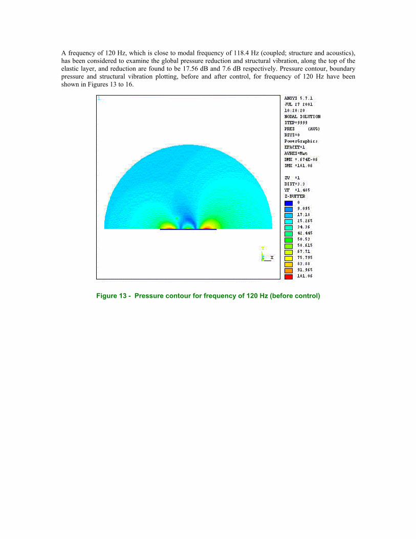
A frequency of 120 Hz, which is close to modal frequency of 118.4 Hz (coupled; structure and acoustics), has been considered to examine the global pressure reduction and structural vibration, along the top of the elastic layer, and reduction are found to be 17.56 dB and 7.6 dB respectively. Pressure contour, boundary pressure and structural vibration plotting, before and after control, for frequency of 120 Hz have been shown in Figures 13 to 16.

Figure 13 - Pressure contour for frequency of 120 Hz (before control)

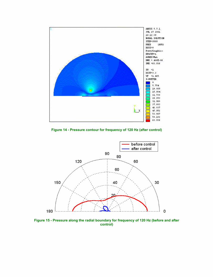
Figure 14 - Pressure contour for frequency of 120 Hz (after control)

Figure 15 - Pressure along the radial boundary for frequency of 120 Hz (before and after control)

Figure 16 - Displacement along the top of the elastic layer for frequency of 120 Hz (before and after control)

Conclusion: Acoustic field and the strength of source used in ANSYS have been described and the result of various cases associated with the acoustic pressure field creation has been compared with the analytical result. All results are in good agreement with the analytical outcome. This study provides a clear view of the acoustic noise field generation in the commercial finite element code, ANSYS. For 2-D acoustic FEM of ANSYS, the acoustic point source is cylindrical point source. The radius of circular infinite boundary is crucial for the FEM results. Active control of structurally radiated sound into a fluid medium has also been implemented in ANSYS where piezo electric material is used as a controlling tool. The cost function that was minimized is the sum of the squared sound pressures at the nodes in the fluid medium. A simple control system with multiple piezoelectric actuators is able to reduce the global sound level. It can be concluded that minimization of sound field radiated by a source for a given excitation frequency can be achieved using multiple piezo elements in ANSYS. The active control study reported in this paper is preliminary which is limited to the active reduction of sound in single frequency and 2-D model with small number of piezo elements. 3-D model and multi-frequency noise reduction with active actuator can be simulated for the future study.

Reference: 1) G. R. Liu, C. Cai, X. M. Zhang and K. Y. Lam, Effects of Piezocomposite Coating on Sound

Radiation and Scattering by a Submerged Cylindrical Structure, 70th shock and Vibration Symposium Nov. 15-19, 1999, USA (Albuquerque, NM).

2) ANSYS, Acoustic and Fluid-Structure Interaction, A Revision 5.0 Tutorial, ANSYS, Inc., June 1992.

3) ANSYS, "Theory Reference, Release 5.7," ANSYS, Inc., March. 2001.

4) P. M. Morse and K. U. Ingard, Theoretical Acoustics, New York: McGraw-Hill, Inc., 1968, pp-358.

5) Miguel C. Junger and David Feit, “Sound, Structures and their interaction”, Cambridge, Mass,

MIT press, 1972.