A Theoretical Analysis of the Lean Startup’s Product ...

Submitted to

A Theoretical Analysis of the Lean Startup’s ProductDevelopment Process

Onesun Steve YooUCL School of Management, University College London, London E14 5AB, United Kingdom, [email protected]

Tingliang HuangCarroll School of Management, Boston College, Chestnut Hill, MA 02467, USA, {[email protected]}

Kenan ArifogluUCL School of Management, University College London, London E14 5AB, United Kingdom, [email protected]

The widely-touted Lean Startup method is emerging as a best practice for entrepreneurs’ early product

development, and it is also featured in entrepreneurship curriculums in academia. Central to its paradigm

is that startups should iteratively launch minimum viable products (MVPs) to gather consumer feedback

and then modify (or “pivot”) the product design goals in response to that feedback. This approach purport-

edly helps entrepreneurs to efficiently learn and develop what consumers want. Despite its influence in the

entrepreneurship and academic communities, there is to date no theoretical formalization for the effectiveness

of the Lean Startup. Some practitioners experience difficulty implementing it in practice, and researchers

question its generalizability. This paper attempts to fill this void by presenting and analyzing a stylized

model of the Lean Startup’s product development process. We find that the Lean Startup’s effectiveness in

learning about consumer tastes is highly dependent on the entrepreneur’s choice of the quality of the MVP.

We also characterize how the potential benefit and implementability (robustness and feasibility) of the Lean

Startup depend on the product–market environment.

Key words : lean startup, entrepreneurship, new product development, Bayesian learning

1. Introduction

A chief aim of the entrepreneur is to understand consumer needs and deliver what they

want to the market. Successful pursuits lead to financial rewards for the entrepreneur and

positive changes for society (Schumpeter 1934). Yet this is also a fundamental challenge for

entrepreneurs, because it is difficult to know exactly which future innovation consumers

will be willing to adopt, not least because consumers seldom know themselves.

The Lean Startup method is a conceptual paradigm aimed at helping entrepreneurs

tackle this challenge. Its key mechanism is learning what consumers want by iteratively

(a) launching products with important but underdeveloped attributes—minimum viable

1

Author: Analysis of the Lean Startup2 Article submitted to ; manuscript no. (Please, provide the mansucript number!)

products (MVPs)—to acquire feedback and then (b) modifying the initial development

goals—or pivoting—to meet consumer needs (Blank 2013). Compared to the traditional

“waterfall” development process, the Lean Startup paradigm is beneficial because it encour-

ages startups to learn quickly from MVP failures and thus reduce the time and resources

that would otherwise be wasted on developing the wrong product (see Figure 1). This

paradigm has effectively replaced the previous practice and teaching of business planning

(e.g., Delmar and Shane 2003) and has also lowered the cost of starting a company (Hell-

mann and Thiele 2015). Blank (2013) claims that “using lean methods across a portfolio

of startups will result in fewer failures than using traditional methods” (p. 7).

Figure 1 “Traditional” versus “Lean Startup” approach to product development (adapted from Blank 2013).

��

��

��

� ��

��

��

� ��

��

� ��

��

��

� ��

��

��

� � ��

� ��

� ��

��

��

��

��

� � ��

� ��

� ��

� � ��

� ��

��

��

� ��

��

Despite its influence in practice and in academic curriculums, there is to date no theo-

retical foundation for examining the effectiveness of the Lean Startup method. This raises

two important concerns. First, it is unclear how the Lean Startup method should be imple-

mented in practice to maximize its benefits. Practitioners often report that it is challenging

to gather useful feedback through early versions of the product (Hokkanen et al. 2015,

Hokkanen et al. 2016), and they have difficulty progressing the MVP towards the final

product that consumers seek (Bosch et al. 2013, Dennehy et al. 2016). There is presently no

guidance regarding which MVP should be developed and launched. Also, the term “mini-

mum” in MVP suggests that the lower the quality of the MVP, the better it is. But does

the quality of the MVP influence its effectiveness? If so, how? A better theoretical under-

standing can help us better understand the challenges of implementing the Lean Startup

approach and help entrepreneurs maximize the benefit from this approach.

Author: Analysis of the Lean StartupArticle submitted to ; manuscript no. (Please, provide the mansucript number!) 3

Second, the extent to which the Lean Startup method is applicable in different settings

is unclear. Teece et al. (2016) observe that the Lean Startup implicitly deals with “cir-

cumstances where development (and adjustment) costs are relatively low, the decisions are

not irreversible (e.g., as in capacity investments), and rapid feedback from customers and

learning is possible ... it is suitable for software entrepreneurs targeting consumer mar-

kets, but less so for aircraft or automobile industries” (p. 26). It is also not suitable if an

entrepreneur’s innovation is closely monitored by the competition (Mihm et al. 2015). Even

in settings where applying the Lean Startup method appears to be suitable—i.e., those

with a low cost, a high level of consumer feedback, and minimal competitive monitoring—it

may not be. A theoretical formalism can help refine our understanding of when the Lean

Startup approach is most suitable in terms of potential benefit and implementability.

In this paper, we aim to address the lack of a theoretical formalism by presenting a

stylized model of the Lean Startup product development process. We employ a spatial

differentiation model (i.e., a Hotelling model) where consumers are heterogeneous in their

horizontal preferences (i.e., taste). Consumer tastes are clustered around a collection of

attributes (or a design), but the entrepreneur does not know this design’s location in the

attribute space. Developing the product that maps onto this design location results in high

profit (i.e., it is the “ideal product”), and to accomplish this, the entrepreneur must learn

through launching MVPs. Specifically, the entrepreneur makes decisions about which MVP

to launch and what its quality should be and then, depending on the sales outcome for

the MVP, the entrepreneur updates his or her belief in a Bayesian manner and determines

whether to continue developing the MVP to a full product or to “pivot” and develop a

different product.

The model’s analysis addresses the two previously cited concerns. First, it reveals insights

into the operational-level decisions that can facilitate successful implementation. Regarding

the joint choice of an MVP and its quality, we find that the entrepreneur should launch the

MVP of the product that he or she thinks is more likely to become the ideal product. We

also isolate the benefit of the Lean Startup. We find that the Lean Startup is less beneficial

to an entrepreneur who has a strong prior belief. Interestingly, we also find that the benefit

of the Lean Startup is nonmonotonic in the quality of the MVP, with an intermediate

MVP quality revealing the most information about consumer tastes. In other words, in


contrast to the connotation suggested by “minimum,” the vertical quality of the MVP

plays a significant role for learning about consumers’ horizontal tastes.

Second, our parsimonious model reveals how the product–market environment (i.e., the

parameter settings) impacts the potential benefit of the Lean Startup. In some settings,

the benefit of the Lean Startup can be marginal even when it is optimally implemented

by the entrepreneur (with an optimal choice of the MVP and its quality). Our model

also provides insights regarding the practical implementability of the Lean Startup in

terms of its robustness and feasibility. In particular, we observe that in some settings,

the benefit of the Lean Startup will fall sharply when the launched MVP quality deviates

from the optimal quality and that in other settings, the benefit of the Lean Startup will

be nonexistent unless the entrepreneur launches a high-quality MVP. We examine the

impact of each model parameter on the potential benefit and implementability of the Lean

Startup and find that although the roles of some parameters are straightforward, others

are more complex. For example, when the potential product designs that the entrepreneur

is considering differ more from each other, the potential benefit of the Lean Startup always

increases. However, an increase in the level of heterogeneity in consumer tastes increases

the potential benefit of the Lean Startup, but it also makes it less robust. Our model

thus presents insights regarding the product–market environments where the Lean Startup

approach should be encouraged.

2. Literature Review

The Lean Startup focuses on the concept development stage in the new product develop-

ment process, where firms learn about consumer preferences (Krishnan and Ulrich 2001).

It marries the two concepts of early consumer engagement and agile development in the

entrepreneurial setting (Ries 2011, Blank 2013) and thus presents a unique framework that

deserves formal enquiry. We examine how our work relates to the streams of the literature

on marketing, new product development, and operations management.

Engaging consumers and learning about their preferences in the new product concept

stage is a central theme in the field of marketing that has been extensively studied. One

of the predominant approaches uses multiattribute models of consumer preferences and

estimates the preference models’ parameters. Conjoint analysis is a well-researched method

for extracting consumer preferences for different attributes by asking them to evaluate a


set of alternatives (Green and Srinivasan 1978, Green and Srinivasan 1990). The method is

widely adopted in practice (Mahajan and Wind 1992), and its application domain has been

extended to include managers’ prior beliefs (Sandor and Wedel 2001), consumer learning

(Yu et al. 2011), and mental simulation and analogies for choices involving really new prod-

ucts (Hoeffler 2003). Another approach is to use internet-based crowds, e.g., to test product

concepts using virtual images (Dahan and Srinivasan 2000) or to extract ideas from the

community of consumers (crowdsourcing) (Bayus 2013). In these studies, the fundamental

approach is to learn about consumer preferences without the actual product. In contrast,

the Lean Startup method promotes learning by selling an MVP for a marginal price and

receiving feedback about the product from the actual customers. This approach allows

customers to use the product or service and enables entrepreneurs to learn by observing

consumer purchase behavior. Also, while these studies examine estimation techniques, our

study employs a stylized analytical model to aid the implementation of the Lean Startup

approach to learning.

Our work is relevant to a stream of the marketing literature that incorporates consumer

utility models and analyzes the impact of consumer heterogeneity. Consumer heterogeneity

has been characterized along either the vertical or horizontal dimension. In the product

line design literature, consumers are heterogeneous in their preferences for vertical quality,

and firms must make their vertical quality assortment decision considering potential canni-

balization (Mussa and Rosen 1978, Moorthy 1984, Villas-Boas 1998, Netessine and Taylor

2007). In contrast, the Lean Startup is more concerned with entrepreneurs in the early

stages of learning about consumer tastes (horizontal quality) and deciding on one product

rather than a line of products. Our modeling approach is therefore more consistent with

various spatial differentiation models where customers are assumed to be heterogeneous

in their horizontal taste preferences (Hotelling 1929). These models have been applied in

marketing and operations management settings to study the impact of taste heterogene-

ity on a firm’s product introductions, pricing, and advertising decisions (Lancaster 1990,

Grossman and Shapiro 1984, Soberman 2004, Kinshuk et al. 2010). We apply such a model

to the study of Lean Startups. Specifically, we assume that the center of consumer tastes

is unknown to the entrepreneur and examine how the entrepreneur can learn consumer

tastes by launching MVPs.


The setting of sequential learning in the early stages of product development has been

studied by a vast literature on new product development. In particular, Thomke (1998)

views experimentation as a fundamental innovation process activity and examines its role

in product design. Other studies examine the efficacy of the sequential trial and error

method compared to parallel learning (Loch et al. 2001), how the results of this comparison

are influenced by complexity and uncertainty (Sommer and Loch 2004), and how design

complexity influences the number of experiments (Erat and Kavadias 2008). A related

mechanism for learning is for firms to hold innovation tournaments to come up with the

“best idea” for product designs (Terwiesch and Ulrich 2009, Girotra et al. 2010). The

primary focus of this literature is, however, how firms can arrive at the optimal (or a

feasible) functional solution for a product (e.g., the algorithm for Netflix), with the func-

tional aim of the product typically assumed to be fixed. In contrast, in the setting of the

Lean Startup, entrepreneurs learn about consumer tastes, and the product to be devel-

oped often changes as a result of the learning. Moreover, in the entrepreneurial setting,

parallel testing or determining a portfolio of products is not part of the decision set. Ter-

wiesch and Loch (2004) examine the setting of collaborative prototyping where the firm

and customer jointly search for the ideal specification. Their study, however, considers a

single consumer (e.g., an architect and her client) and focuses on potential agency issues.

Our setting does not involve agency issues but instead focuses on identifying the central

preference of consumers who are not strategic.

A key framework widely employed in the new product development literature uses search

models (Weitzman 1979, Massala and Tsetlin 2015). The key trade-off in the search liter-

ature is between the cost of the search and the expected benefit of continuing the search.

While conceptually similar to a search problem, our model fundamentally differs in two

respects. First, our key trade-off does not hinge on the cost component. Instead, we exam-

ine how the vertical quality of launched MVPs can influence the information value (for

learning about horizontal taste) of their sales outcome. Specifically, everybody (nobody)

will purchase an MVP if the quality is too high (too low), regardless of whether it contains

the ideal features, which leads to little information coming from the sales outcome. Second,

unlike in search models, where the searcher observes the true value of an alternative, in

our setting the entrepreneur observes a noisy signal about consumer taste. Thus, our form


of learning is similar to sequential experimentation models that employ Bayesian updating

of beliefs using sample information.

Sequential updating models, such as partially observed Markov decision processes or

multiarmed bandit models, are widely used in the operations management literature in

the context of inventories (Scarf 1959, Iglehart 1964, Azoury 1985, Larson et al. 2001),

dynamic pricing (Aviv and Pazgal 2005, Harrison et al. 2012), and dynamic assortment

(Caro and Gallien 2007, Caro and Yoo 2010). Although these models examine learning

regarding an unknown parameter (e.g., inventory demand), it is not linked to consumers’

taste. Ulu et al. (2012) do examine the retail assortment decision based on learning about

consumer taste; however, our study is the first to examine how an entrepreneur can use

the vertical quality of an MVP to learn about horizontal preferences for the new product.

Finally, the sequential launch of MVPs is similar to firms’ launches of newer versions of

the same product (e.g., iPhone versions). For example, Bhaskaran et al. (2013) examine how

start-ups should sequentially launch products to generate revenue to balance innovation

and survival, while Lobel et al. (2016) study how firms should launch new versions of

existing products when consumers are strategic. The decision concerning MVP launches is,

however, fundamentally different, because its objective is not to earn revenue, but rather

to learn about consumer tastes.

3. Model

In our model, the entrepreneur first develops and launches a product, and then the con-

sumers decide whether to purchase the product based on its fit with their tastes. Demand

will be high (low) if the launched product has a good (poor) fit with consumer taste, and

thus the entrepreneur seeks to develop a product that consumers want. In this section,

following the spirit of backward induction, we first characterize consumer adoption and

market demand based on the product’s fit with the consumers’ taste (§3.1), followed by

the entrepreneur’s implementation problem (§3.2).

3.1. Consumer Purchase Decision and Aggregate Market Demand

To model heterogeneity in consumers’ horizontal preferences (taste), we employ the spatial

differentiation model (Hotelling 1929, Grossman and Shapiro 1984). For simplicity, we

assume a product design with a single attribute. A consumer’s taste is represented by

the consumer’s position x ∈ (−∞,∞) on the attribute line and is the consumer’s private


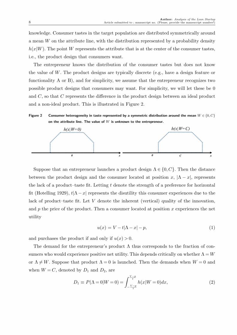
knowledge. Consumer tastes in the target population are distributed symmetrically around

a mean W on the attribute line, with the distribution represented by a probability density

h(x|W ). The point W represents the attribute that is at the center of the consumer tastes,

i.e., the product design that consumers want.

The entrepreneur knows the distribution of the consumer tastes but does not know

the value of W . The product designs are typically discrete (e.g., have a design feature or

functionality A or B), and for simplicity, we assume that the entrepreneur recognizes two

possible product designs that consumers may want. For simplicity, we will let these be 0

and C, so that C represents the difference in the product design between an ideal product

and a non-ideal product. This is illustrated in Figure 2.

Figure 2 Consumer heterogeneity in taste represented by a symmetric distribution around the mean W ∈ {0,C}

on the attribute line. The value of W is unknown to the entrepreneur.

0 x

0 x

h(x|W=0)

h(x|W=C)

C

0 x

0 x

h(x|W=0)

h(x|W=C)

C

Suppose that an entrepreneur launches a product design Λ ∈ {0,C}. Then the distance

between the product design and the consumer located at position x, |Λ− x|, represents

the lack of a product–taste fit. Letting t denote the strength of a preference for horizontal

fit (Hotelling 1929), t|Λ−x| represents the disutility this consumer experiences due to the

lack of product–taste fit. Let V denote the inherent (vertical) quality of the innovation,

and p the price of the product. Then a consumer located at position x experiences the net

utility

u(x) = V − t|Λ−x| − p, (1)

and purchases the product if and only if u(x)> 0.

The demand for the entrepreneur’s product Λ thus corresponds to the fraction of con-

sumers who would experience positive net utility. This depends critically on whether Λ =W

or Λ 6=W . Suppose that product Λ = 0 is launched. Then the demands when W = 0 and

when W =C, denoted by D1 and D2, are

D1 ≡ P (Λ = 0|W = 0) =

∫ V−pt

−V−pt

h(x|W = 0)dx, (2)


D2 ≡ P (Λ = 0|W =C) =

∫ V−pt

−V−pt

h(x|W =C)dx. (3)

This is illustrated in Figure 3. The left panel represents the case where the mean W is

0, which is equal to the entrepreneur’s product Λ (= 0). In this case, all of the consumers

have positive utility, and so the entrepreneur will capture the entire market. The right

panel represents the case where the mean W is C, which does not correspond to the

entrepreneur’s product Λ (= 0). In this case, only a fraction of the consumers (those located

to the left of (V − p)/t)) have positive utility, and consequently the entrepreneur will lose

the remaining fraction of potential consumers.

Figure 3 Impact of location (Λ) on demand. The solid lines represent the utility function u(x) = V − t|Λ−x|−p.

Assuming that the entrepreneur develops Λ = 0, the left panel illustrates the case where W = 0 and

the right panel W =C.

�

��

��

��

��

�

��

��

��

��

Clearly, D1 >D2, and thus, developing a product Λ =W can be thought of as developing

the “ideal product.” Due to the symmetry of the distribution h(x|W ), we have P (Λ =

C|W =C) = P (Λ = 0|W = 0) =D1 and P (Λ =C|W = 0) = P (Λ = 0|W =C) =D2. In other

words, D1 represents the demand when the entrepreneur launches the ideal product, and

D2 represents the demand when the entrepreneur launches a non-ideal product.

3.2. The Entrepreneur’s Lean Startup Implementation Problem

The entrepreneur aims to develop a product Λ that matches the center of the consumers’

tastes, W . In the early product development process, when the entrepreneur does not know

whether W = 0 or W =C, he or she has a prior belief, namely, P (W = 0) = r. Consistent

with the Bayesian assumption that beliefs and outcome probabilities are equivalent, when

the entrepreneur develops product Λ = 0 (or, equivalently, Λ =C), it will result in the ideal

product with probability r, and a non-ideal product with probability 1− r.In implementing the Lean Startup approach, the entrepreneur aims to improve the prob-

ability of launching the ideal product. The key mechanism of the Lean Startup is learning


from the MVP. Recall that an MVP is a product that contains the key attributes of the

final product, but is underdeveloped. In other words, an MVP (denoted λ) occupies the

same locations on the attribute line as the final product (Λ) would, but has a quality v

that is lower than that of the final product (V ).

Implementation of a Lean Startup requires the entrepreneur to decide which MVP λ ∈

{0,C} to develop, along with its quality v ∈ [0, V ]. Since the entrepreneur launches the

MVP at a marginal price, we assume for simplicity that the price of the MVP is set to

zero. Also, developing an MVP requires fewer resources and less lead time than developing

the full product. For simplicity, we assume that launching an MVP and pivoting (or not

pivoting) has a fixed cost K.

After an MVP is launched, sales are observed. For simplicity, we assume that a single

consumer1 with location x is randomly picked from the consumer distribution h(x|W ) and

that the consumer decides to purchase the MVP based on whether or not his or her net

utility from obtaining the MVP is positive, i.e., u(x) = v − t|λ − x| ≥ 0. The MVP can

either generate a sale or lead to no sale. If the MVP λ= 0 was launched, the probabilities

that a randomly selected customer will purchase the MVP when W = 0 and when W =C,

respectively denoted by q1(v) and q2(v), are:

q1(v) ≡ P (λ= 0 & sale|W = 0) =

∫ v/t

−v/th(x|W = 0)dx, (4)

q2(v) ≡ P (λ= 0 & sale|W =C) =

∫ v/t

−v/th(x|W =C)dx. (5)

The probabilities (4)-(5) are determined the same way as the demands in (2)-(3). In Fig-

ure 3, they can be represented by replacing the final quality V with the MVP quality v,

the price p with 0, and the product location Λ with λ.

Due to the inherent randomness in the selection of a customer, even launching an ideal

MVP (λ=W ) can lead to no sale when the selected consumer’s taste is located far away

from W . Similarly, launching a non-ideal MVP (λ 6=W ) can lead to a sale when the selected

consumer’s taste is located close to λ. Nevertheless, developing and launching the MVP

of the ideal product will have a higher chance of generating a sale, and thus the sales

outcome yields information. Specifically, after observing the sales outcome for MVP λ= 0,

1 One can easily generalize to an arbitrary number of samples, but with additional complexity.


the entrepreneur’s prior belief r = P (W = 0) will be updated according to Bayes’ rule as

follows:

P (W = 0|λ= 0 & sale) =P (λ= 0 & sale|W = 0)P (W = 0)

P (λ= 0 & sale|W = 0)P (W = 0) +P (λ= 0 & sale|W =C)P (W =C)

=q1(v)r

q1(v)r+ q2(v)(1− r). (6)

Similarly, there are three other possible updated beliefs, depending on which MVP λ ∈

{0,C} was launched and whether or not a sale occurred:

P (W = 0|λ= 0 & no sale) =(1− q1(v))r

(1− q1(v))r+ (1− q2(v))(1− r), (7)

P (W =C|λ=C & sale) =q1(v)(1− r)

q1(v)(1− r) + q2(v)r, (8)

P (W =C|λ=C & no sale) =(1− q1(v))(1− r)

(1− q1(v))(1− r) + (1− q2(v))r. (9)

If the MVP λ= 0 (or λ=C) resulted in a sale, then the entrepreneur’s belief that W = 0

(or W =C) is raised, and it may be optimal to continue developing the product attributes

to full quality and launch the product Λ = 0 (or Λ = C). If the MVP resulted in no sale,

then the entrepreneur’s belief that W = 0 (or W = C) is lowered, and it may be optimal

to “pivot” and develop and launch Λ =C (or Λ = 0) instead. The entrepreneur’s objective

is to maximize the expected profit from the final product launch by (a) deciding which

MVP to launch and with what quality, and (b) determining whether or not to pivot after

observing the sales outcome for the MVP. The sequence is represented in Figure 4.

Figure 4 Sequence of events.

Entrepreneur’s decisions: •  Which MVP to launch? •  What quality v?

Entrepreneur has prior belief about ideal product, P(W=0)=r.

Entrepreneur’s decision: •  Continue development

or pivot?

MVP sale outcome realized, and entrepreneur updates belief about ideal product

Final product sale outcome and profit realized

time

To understand the learning dynamics, we will consider a single iteration (§5.1 examines

the impact of multiple iterations). To focus on learning, we assume that the values V


and p are exogenously given. One can consider pricing as a secondary decision when it is

determined either by consumer demand or technology/cost constraints in the market place.

(We will show in §5.2 that the results are robust when prices are endogenous.) By definition,

developing an MVP and then pivoting requires minimal development/adjustment costs,

so for simplicity, we will assume these costs are zero. (We will discuss the impact of the

development and adjustment costs in §5.3).

4. Analysis of the Lean Startup

We present the structural results for the optimal implementation policy in §4.1 and examine

the Lean Startup’s potential benefit and implementability in §4.2.

4.1. Structure of the Optimal Policy

Using backward induction, we first examine the entrepreneur’s optimal pivoting decision

after observing the sales outcome for the MVP.

Lemma 1 (Optimal Pivoting). Suppose that the entrepreneur launched the MVP λ=

0 (or λ= C) with quality v, and let r̃ represent the posterior belief that the ideal product

W is 0 based on (6)–(7) (or (8)–(9)). Then it is optimal to pivot if and only if r̃ < 0.5 (or

r̃ > 0.5).

Lemma 1 shows that it is optimal to pivot if, after observing the MVP sale outcome,

the entrepreneur believes that there is a higher probability that the other product is the

ideal product. From expressions (6)–(9), we observe that the posterior belief r̃ depends on

which MVP λ∈ {0,C} was launched, its quality, and the prior belief r.

Let πLS(λ, v|r) denote the expected profit when applying the Lean Startup with MVP

λ∈ {0,C} and quality v ∈ [0, V ] given the prior belief P (W = 0) = r, assuming that optimal

pivoting occurs. The next result shows the relationship between the optimal MVP choice

and its quality as well as the expression for the optimal expected profit.

Proposition 1 (Optimal MVP Choice and Quality, and Expected Profit).

(i) The optimal MVP choice λ∗ depends on the quality v, as follows:

λ∗(v) =

0, v≥ v̄

C, v≤ v̄if r≥ 0.5, λ∗(v) =

C, v≥ v̄

0, v≤ v̄if r < 0.5,


where v̄ is such that q1(v) + q2(v) = 1 for v= v̄. (ii) The optimal expected profit is given by

πLS(λ∗(v), v|r) =

(r+β(v|r))D1p+ (1− r−β(v|r))D2p, r≥ 0.5,

(1− r+β(v|r))D1p+ (r−β(v|r)))D2p, r < 0.5,

where, letting [a]+ ≡max{0, a},

β(v|r) ,

min{

[1− 2r+ rq1(v)− (1− r)q2(v)]+, [(1− r)q1(v)− rq2(v)]+}, r≥ 0.5,

min{

[2r− 1 + (1− r)q1(v)− rq2(v)]+, [rq1(v)− (1− r)q2(v)]+}, r < 0.5.

The first part of the proposition reveals that the entrepreneur should either launch the

MVP for the product design that he or she believes is more likely to be the ideal product

(λ= 0 if r ≥ 0.5 or λ=C if r < 0.5) at a high quality (v ≥ v̄) or launch the MVP for the

product design that he or she believes is not likely to be the ideal design (λ=C if r≥ 0.5

or λ = 0 if r < 0.5) at a low quality (v ≤ v̄). Suppose that the prior belief r is greater

than 0.5. Then launching an MVP that is more likely to be ideal at a low quality v < v̄ is

suboptimal because its probability of a sale, q1(v), is lower than the probability of having

no sale when launching a non-ideal product, 1− q2(v). It is preferable to launch either a

higher quality MVP (v > v̄) that is more likely to be the ideal product or a lower quality

MVP (v < v̄) that is more likely to be a non-ideal product.

The second part of the proposition reveals that implementing the Lean Startup devel-

opment process increases the entrepreneur’s probability of attaining the ideal product

(demand case D1) by β(v|r), compared to the probability based on the entrepreneur’s prior

belief, max{r, 1 − r}. Thus, we will refer to the term β(v|r) as the benefit of the Lean

Startup.

The next two results examine how the benefit β(v|r) is influenced by the entrepreneur’s

prior belief r and the choice of the MVP quality v.

Corollary 1 (Impact of the Prior Belief r). For any v, the benefit of the lean

Startup is the greatest when r= 0.5 and decreases as r→ 0 or r→ 1.

This is intuitive. The entrepreneur will benefit the most when the strength of his or

her prior belief, max{r, 1− r}, is the lowest, i.e., when r= 0.5. If, on the other hand, the

entrepreneur has a strong prior belief, i.e., when r is sufficiently far from 0.5, it may be

undesirable to learn, considering the cost K > 0 of implementing the Lean Startup process.


Next, we note that for any prior belief r, the expression β(v|r) contains the weighted

difference ρq1(v)− (1− ρ)q2(v), for ρ ∈ [0,1]. Thus, maximizing the benefit of the Lean

Startup requires choosing the quality v of the MVP. Recalling that we did not assume any

cost associated with the development of the MVP, it may appear that launching a higher

quality MVP should always be beneficial. Our next result shows that this is not the case.

Corollary 2 (Nonmonotonic Impact of MVP Quality v). For any r, the bene-

fit of the Lean Startup is increasing-decreasing (i.e. unimodal) in v.

The intuition for Corollary 2 is as follows. Suppose that v is high. Then all consumers

will purchase the MVP regardless of whether it is the MVP of the ideal product or not,

i.e., q1 = q2 = 1. In such a case, the probability updating according to the Bayesian rule in

Eqs. (6) and (8) results in little change and therefore no learning. Similarly, if v is low, no

consumer will purchase the MVP regardless of whether it is the MVP of the ideal product,

i.e., q1 = q2 = 0. Such a setting again leads to little probability updating in Eqs. (7) and

(9) and hence no learning.

In sum, there is a range of quality values for the MVP that the entrepreneur can choose

from when implementing the Lean Startup. While the connotation given by “minimum”

suggests that choosing the lowest value possible is desirable, Corollary 2 shows that doing

so will not lead to maximal learning. The effectiveness of the Lean Startup is typically

maximized for some nonlimiting value of the MVP quality v.

4.2. Potential Benefit and Implementability of the Lean Startup

Considering the cost of implementing the Lean Startup (K ≥ 0), it is important to under-

stand the potential benefit it can achieve. Also, in terms of implementation, it may be

challenging for the entrepreneur to select the precise optimal quality v∗ for the MVP (e.g.,

due to the modularity of systems or because it is too high relative to the full quality V ). If

the benefit of the Lean Startup drops sharply as the entrepreneur deviates from the optimal

quality v∗, the actual benefit attained in practice will likely be low. It would also be less

feasible to implement the Lean Startup if its benefit is small unless a high-quality MVP is

launched. In this section, we examine how the product–market environment influences the

Lean Startup’s potential benefit and its implementability.

To attain clear insights, we assume that consumers are distributed uniformly along the

attribute line between W − ε and W + ε for some W ∈ {0,C}, ε ≥ C/2. The inequality


ensures that there is some overlap between the two distributions h(x|W = 0) and h(x|W =

C). The expressions for the demand for ideal and non-ideal products (2)-(3), and those for

the probability of a sale of ideal and non-ideal MVPs (4)-(5) are, respectively:

D1 = min

(V − pεt

, 1

), D2 = min

([V − p

2εt− (C − ε)

2ε

]+, 1

); (10)

q1(v) = min( vεt, 1), q2(v) = min

([v

2εt− (C − ε)

2ε

]+, 1

). (11)

The next result presents the optimal MVP choice λ∗ and quality v∗, along with the

expected profit.

Proposition 2 (Optimal Policy). Suppose that h(x|W ) is uniformly distributed in

[W − ε,W + ε] for some W ∈ {0,C} and ε > C/2. Then it is optimal to launch the MVP

λ∗ = 0 (λ∗ =C) when r≥ 0.5 (r < 0.5) and to set the quality v∗ = εt. Moreover,

πLS(λ∗(v), v∗ = εt|r) =

(r+β(v∗|r))D1p+ (1− r−β(v∗|r))D2p, r≥ 0.5,

(1− r+β(v∗|r))D1p+ (r−β(v∗|r))D2p, r < 0.5,(12)

where

β(v∗ = εt|r) =

(1− r)(1− q2(εt)), r≥ 0.5,

r(1− q2(εt)), r < 0.5.(13)

The proposition states that it is optimal to launch the MVP of the product that the

entrepreneur thinks is more likely to be the ideal product, and to always set its quality

to v∗ = εt. For the uniform case, due to the piecewise linearity of the weighted difference

between q1(v) and q2(v), it is interesting to note that any marginal change in r does not

influence the value v∗ of the optimal MVP quality.

We examine the intuition behind the optimal MVP quality v∗. From (11), the optimal

level of the MVP quality v∗ = εt is such that if the MVP that was launched represents the

ideal product, then all consumers will purchase it (q1 = 1), and if it represents a non-ideal

product, some consumers may not purchase it (q2 = 1− C2ε

). In other words, if the MVP

with the optimal quality v∗ leads to no sales, then this will reveal that the entrepreneur

is developing a non-ideal product. In this case, the entrepreneur can pivot to develop the

ideal product.


To examine how the product–market environment impacts the Lean Startup’s potential

benefit and implementability, we next consider an entrepreneur who has a prior belief

r = 0.5, which is when the benefit of the Lean Startup is potentially the highest. When

r= 0.5, the choice of λ∈ {0,C} is indifferent, and the expression simplifies to

β(v|r= 0.5) =q1(v)− q2(v)

2.

The next proposition examines its comparative statics.

Proposition 3 (Comparative Statics). Suppose that h(x|W ) is uniformly dis-

tributed in [W − ε,W + ε] for some W ∈ {0,C}, ε >C/2. Then:

(i) maxv β(v|r= 0.5) = C4ε

;

(ii) ∂∂v|β(v|r= 0.5)| |v=v∗= 1

4εt;

(iii) V − arg maxv β(v|r= 0.5) = V − εt.

The first part of Proposition 3 shows that the potential benefit of the Lean Startup

increases in C and decreases in ε. The intuitions are as follows. First, recall that the

parameter C denotes the difference between the two product designs that the entrepreneur

thinks may be the ideal product. The parameter ε of the uniform distribution denotes

the range of the consumers’ taste distributions. A high C or low ε indicates that the two

distributions overlap less, and therefore a sale (or no sale) of an MVP can be attributed

more to whether the MVP of the ideal product (non-ideal product) was launched and less

to the random selection of a customer who was offered the MVP. In other words, the ratio

C/ε can be interpreted as the signal-to-noise ratio, and a higher ratio signifies that the

MVP sales outcome provides more information, making the Lean Startup potentially more

beneficial.

The second part of Proposition 3 shows that the Lean Startup is highly sensitive to

the choice of the MVP quality v when the quantity εt is low, or equivalently, that it is

more robust when εt is high. Recall that the parameter t represents the strength of the

consumer’s horizontal preferences (or tastes). A low t implies that consumers will purchase

primarily based on the vertical quality. In such a case, discerning the consumers’ horizontal

preferences becomes inherently difficult: a small deviation from the optimal MVP quality

v∗ could lead to either all consumers purchasing the product (the MVP will always sell) or

no consumers purchasing the product (the MVP will never sell), depending on the vertical


quality. Similarly, because a low ε indicates that consumer tastes are concentrated around

a product design, this also makes it an “all-or-nothing” proposition for the entrepreneur:

If the MVP quality v is high, the entrepreneur will capture the entire market (the MVP

always sells), regardless of whether or not it represents the ideal product, and if the MVP

quality v is low, the entrepreneur will miss the market entirely (the MVP never sells),

regardless of whether or not the MVP represents the ideal product. Thus, when either ε

or t is low, a small deviation from the optimal MVP quality can result in a significant

reduction in information about the consumers’ tastes.

Finally, the third part of Proposition 3 represents the “slack” in the MVP quality con-

straint. The greater the slack, the more feasible it is to implement the Lean Startup method.

Thus, feasibility increases with smaller ε or t. The contextual dependencies of the Lean

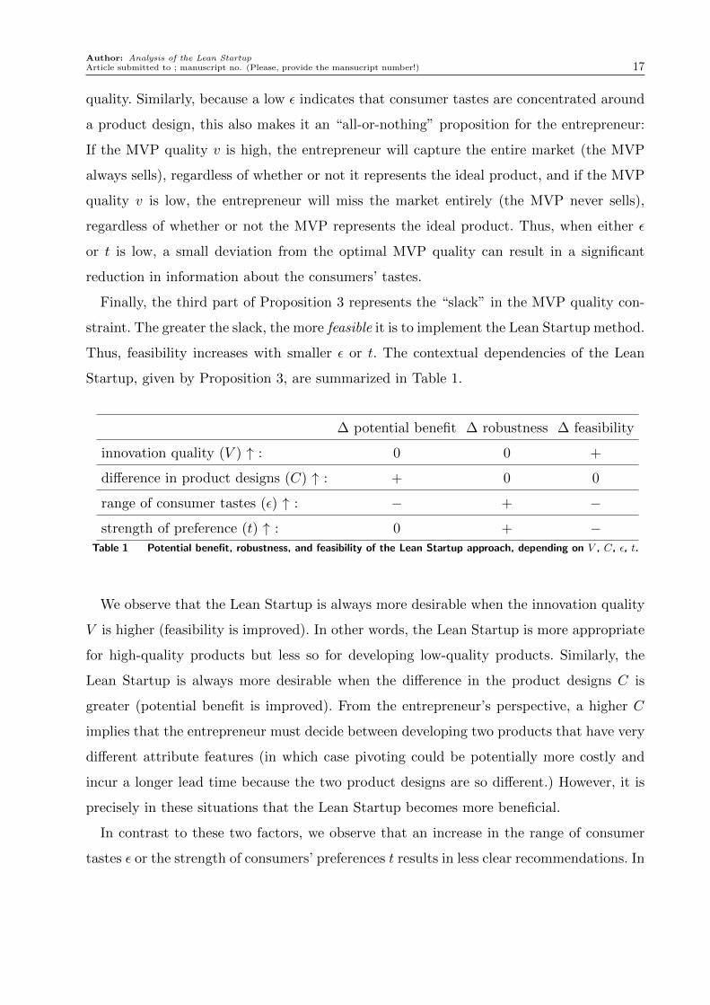
Startup, given by Proposition 3, are summarized in Table 1.

∆ potential benefit ∆ robustness ∆ feasibility

innovation quality (V ) ↑ : 0 0 +

difference in product designs (C) ↑ : + 0 0

range of consumer tastes (ε) ↑ : − + −

strength of preference (t) ↑ : 0 + −Table 1 Potential benefit, robustness, and feasibility of the Lean Startup approach, depending on V , C, ε, t.

We observe that the Lean Startup is always more desirable when the innovation quality

V is higher (feasibility is improved). In other words, the Lean Startup is more appropriate

for high-quality products but less so for developing low-quality products. Similarly, the

Lean Startup is always more desirable when the difference in the product designs C is

greater (potential benefit is improved). From the entrepreneur’s perspective, a higher C

implies that the entrepreneur must decide between developing two products that have very

different attribute features (in which case pivoting could be potentially more costly and

incur a longer lead time because the two product designs are so different.) However, it is

precisely in these situations that the Lean Startup becomes more beneficial.

In contrast to these two factors, we observe that an increase in the range of consumer

tastes ε or the strength of consumers’ preferences t results in less clear recommendations. In


particular, an increase in the range of consumer tastes increases the Lean Startup’s robust-

ness, but it simultaneously hurts its effectiveness and feasibility. Similarly, an increase in

the strength of consumers’ preference increases robustness but at the expense of feasibility.

Figure 5 Potential benefit and implementability of the Lean Startup, depending on (C, ε, t).

0 1 2 3 4 50

0.05

0.1

0.15

0.2

0.25

0.3

0.35

MVP quality (v)

VoLS

(v)

(C,ε,t)=(1,1,0.25)(C,ε,t)=(1,2,3)(C,ε,t)=(2,1.5,1)

β(v|r=0.5)

Note. In the case of the dotted curve, the Lean Startup is too sensitive for implementation. In the case of the dashed

curve, it is not feasible. In the case of the solid curve, it is robust and has a high potential benefit.

Figure 5 illustrates that the potential benefit and implementability of the Lean Startup

are highly dependent on the product–market characteristics. The three curves plot the ben-

efit β(v|r= 0.5) for different values of the parameters (C, ε, t) for a fixed innovation quality

V = 5. The solid curve represents the product–market setting with (C, ε, t) = (2,1.5,1).

This is a setting in which the Lean Startup is most desirable in terms of potential bene-

fit, robustness (robust around v∗ = 1.5), and feasibility (V = 5> εt). Relative to the solid

curve, the dotted curve with setting (C, ε, t) = (1,1,0.25) is relatively unsuitable for the

Lean Startup. Although it is highly feasible and has a comparable potential benefit, it is

highly sensitive to the choice v of MVP quality. A slight miscalibration of the MVP quality

can lead to little or no benefit. Similarly, the dashed curve with setting (C, ε, t) = (1,2,3)

is less desirable for implementing the Lean Startup due to unfeasibility. To attain a benefit

from the Lean Startup in this case, the entrepreneur must launch an MVP whose quality

is too high. If an MVP with low quality is launched, the entrepreneur will enjoy no benefit

from the Lean Startup.


Our parsimonious model helps us understand the settings in which the Lean Startup is

potentially most beneficial and its implementability least challenging.

5. Other Considerations

In this section, we discuss other considerations: (i) multiple iterations of MVP launches,

(ii) endogenous pricing decisions, (iii) the role of development and adjustment costs, and

(iv) comparisons with the traditional approach to product development.

5.1. Multiple Iterations of the MVP Launch

The previous section assumed a single iteration of an MVP launch. In the multiple-iteration

setting, the entrepreneur has the option to launch another MVP after observing the sales

outcome for the first MVP launch and updating his or her belief. In such a setting, would

it be optimal to launch an MVP of the product that is likely not the ideal product? Should

the quality of the MVP increase over time? To gain insight, we examine two iterations

(similar analysis can be carried out for n iterations).

Proposition 4 (Optimal Policy for Two Iterations). Suppose that h(x|W ) is

uniformly distributed in [W − ε,W + ε], ε >C/2. Let λt ∈ {0,C} and vt ∈ [0, V ] denote the

optimal MVP choice and quality in period t∈ {1,2}. The optimal policy is as follows.

Period 1: If r≥ 0.5, launch MVP λ1 = 0 with quality v∗1 = εt; if r < 0.5, launch MVP λ1 =C

with v∗1 = εt.

Period 2: If an MVP sale occurred in period 1, launch the same MVP λ∗1 with the same

quality v∗2 = εt. If a sale did not occur in period 1, this reveals that the current product

is not the ideal product. Thus, pivot and develop the other product without launching an

additional MVP.

The proposition reveals that regardless of the number of iterations, it is optimal in period

1 to launch the MVP of the product that the entrepreneur believes to be the ideal product

with quality v1 = εt. Morever, the multiple iteration setting does not require launching a

different MVP (i.e., λ∗1 = λ∗2) or improving its quality (i.e., v∗1 = v∗2). The following corollary

reveals the maximum benefit of the Lean Startup involving two iterations of MVP launches

when the entrepreneur has a prior belief r.

Corollary 3 (Benefit of Lean Startup with Two Iterations). The benefit of

the Lean Startup with two iterations of MVP launches, β2(v1, v2|r), is given by


β2(v∗1 = v∗2 = εt|r) =

(1− r)(1− [q2(εt)]2), r≥ 0.5,

r(1− [q2(εt)]2), r < 0.5.

When r = 0.5, the benefit of the Lean Startup with two iterations of MVP launches

β2(v∗1 = v∗2 = εt|r= 0.5) is 1−[q2(εt)]2

2. Recall that in the single iteration setting, the benefit of

the Lean Startup β(v∗ = εt|r = 0.5) is 1−[q2(εt)]2

. Thus, the additional iteration of an MVP

launch increases the benefit of the Lean Startup, but it does so in a marginally decreasing

manner.

5.2. Endogenizing Pricing Decision

Thus far, the price of the final product, p, has been exogenously given. However, after

launching an MVP, observing the sales outcome, and deciding whether or not to pivot, the

entrepreneur may determine the price of the final product before launching it. How would

endogenous pricing influence the present results concerning the optimal implementation

of the Lean Startup? Does price optimization influence the choice of the MVP or its

quality? Does the updated belief due to the Lean Startup prompt the entrepreneur to

charge higher/lower prices?

To examine the impact of the pricing decision, we examine the setting of a single iteration

of an MVP launch with pricing. For analytical simplicity, consider the uniform setting

with ε= C, and assume that the entrepreneur has the possibility of optimizing the price

of the final product within the range p ∈ [V − εt, V ]. For this set of parameter values, the

expressions for the demand (10) and probability of an MVP sale (11) for the uniform case

simplify to:

D1(p) =V − pεt

, D2(p) =V − p

2εt; (14)

q1(v) =v

εt, q2(v) =

v

2εt. (15)

These assumptions make the MVP decisions independent of price optimization. The

resulting optimal Lean Startup implementation policy and expected profit with pricing

decisions are provided next.

Proposition 5 (Optimal Policy with Pricing Decisions). Suppose consumer

tastes are uniformly distributed within [W − ε,W + ε], for ε = C, and let p ∈ [V − εt, V ].


The entrepreneur should develop λ= 0 if r≥ 0.5 and develop λ=C if r < 0.5, and should

set the quality at v∗ = εt in either case. Moreover, letting [a]+ ≡max{0, a},

πLS(λ∗(v), v= εt|r) =

(r+ 1−r

2

)p∗D1(p

∗) +((1− r)− 1−r

2

)p∗D2(p

∗), r≥ 0.5,((1− r) + r

2

)p∗D1(p

∗) +(r− r

2

)p∗D2(p

∗), r < 0.5,

where

p∗D1(p∗) = min

{V 2

4εt, V − εt

}, p∗D2(p

∗) = min

{V 2

8εt,V − εt

2

}.

Observe that this expression is equivalent to that in Proposition 2, with the expressions

for the profits pD1(p) and pD2(p) optimized, and setting q2(εt) = 0.5. Adding the pricing

optimization problem in the final step requires solving, for any instance of an MVP launch

λ∈ {0,C} and its sales outcome,

maxpp [Q1(λ, v, r)D1(p) +Q2(λ, v, r)D2(p)] .

The coefficients Q1 and Q2 do not depend on the price, but their values do impact the

pricing decision. Under the assumptions ε=C and p∈ [V − εt, V ], the resulting expressions

arising from the price optimization retain the same structure when substituted in the Lean

Startup optimization problem. However, this is not the case under the general assumptions

ε > C/2 and p ∈ [0, V ], where the pricing decision does interact with the implementation

of the Lean Startup and may impact its optimal policy.

Due to the complexities, general analytical characterization is difficult. However, we

observe, based on extensive numerical investigations, that the interaction arising from the

pricing decision does not contribute significantly to either the decisions about the Lean

Startup or the optimal expected profit that results. In other words, price optimization

adds value by increasing both pD1(p) and pD2(p) (as illustrated in Proposition 5), and

implementing Lean Startup adds value by increasing the probability of attaining the higher

profit pD1(p). Any additional value due to their interaction is marginal.

5.3. Role of Development and Adjustment Costs

Thus far, the cost K has played a marginal role as a parameter of the model. This is

because (i) a low development (adjustment) cost is an implicit condition necessary for the

application of the Lean Startup approach (Teece et al. 2016), and (ii) our research aim is

to examine the Lean Startup’s learning mechanism utilizing the launch of MVPs.


In this section, we examine how the presence of an MVP development cost that is convex

increasing in its quality (K1(v)) and the cost of pivoting (K2) impact the entrepreneur’s

Lean Startup implementation decisions. The next result shows that the cost of pivoting

makes pivoting less desirable to the entrepreneur when implementing the Lean Startup.

Lemma 2 (Optimal Pivoting with Cost). Suppose the entrepreneur has launched

MVP λ = 0 (or λ = C) with some quality v, and let r̃ represent the updated belief that

the ideal product W is 0, depending on the sales outcome, according to Eqs. (6)–(7) (or

(8)–(9)). If there is a positive cost K2 of pivoting, then it is optimal to pivot if and only if

r̃ < r̄ < 0.5 (or r̃ > r > 0.5).

Compared to when there is no cost for pivoting (Lemma 1), the threshold belief for

pivoting is lower in this case (r̄ < 0.5). That is, when there is a cost for pivoting, the

entrepreneur will prefer to continue developing the product that he or she initially believed

in (compared to when there is no cost) due to the friction created by the cost of pivoting.

The next result shows the optimal policy in the presence of an MVP development cost.

Proposition 6 (Optimal MVP Quality with Cost). Let v∗ represent the optimal

MVP quality in the setting without any cost for MVP development (Proposition 1), and let

v+ represent the optimal MVP quality in the presence of a convex increasing development

cost K1(v). Then v+ < v∗.

In the presence of an MVP development cost, the entrepreneur will develop an MVP

that is strictly lower quality than when there is no MVP development cost (Proposition 1).

Moreover, recall that in Proposition 1, when a low-quality MVP is to be developed (v < v̄),

it is preferable to launch the MVP of the product that the entrepreneur believes is less

likely to be the ideal product.

As expected, the presence of development/adjustment costs does impact how the Lean

Startup is implemented and also prevents the entrepreneur from deriving its full benefit.

Nevertheless, our numerical studies suggest that, provided the costs are not too high,

it does not significantly alter the key insights. In other words, our results are robust to

settings where costs do not play a significant role. In settings where the development or

adjustment costs are high, the implementation of the Lean Startup would be driven by the

entrepreneur’s cost considerations, including cash constraints. This decision will involve

different tradeoffs, which deserve a formal enquiry that is outside the scope of this paper.


5.4. Comparison with Traditional Method of Learning

So far, we have examined the benefit of the Lean Startup, measured relative to the

entrepreneur’s prior belief. However, as illustrated by the traditional approach in Figure 1,

the entrepreneur can also develop a product following the traditional approach, which

involves upfront market research to learn about consumer tastes (e.g., conjoint analysis)

followed by focused product development.

We now illustrate how traditional learning can also be represented in the context of our

model. Suppose that the upfront market research leads to a prediction regarding whether

the ideal product W is 0 or C. The accuracy of the prediction can be represented by

a parameter ω ∈ [0.5,1]. Specifically, if the market research predicts W = 0, the proba-

bility that W = 0 is ω, or P (W = 0 |W = 0 & Predicted) = ω. If ω = 0.5, then P (W =

0 |W = 0 & Predicted) = 0.5, and the prediction does not offer any improvement over a coin

flip; if ω = 1, then P (W = 0 |W = 0 & Predicted) = 1, i.e., the prediction leads to perfect

knowledge. This notion of accuracy is consistent with the notion of “targeting accuracy”

employed in the marketing literature (e.g., Chen et al. 2001), which can be measured (e.g.,

using historical data).

For simplicity of illustration, assume that the cost of conducting market research is

zero. The expected profit when employing the traditional method of development with

prediction accuracy ω and prior belief r, denoted by πT (ω|r), is as follows.

Proposition 7. The expected profit using the traditional development approach is

πT (ω|r) =

(r+α(ω|r))D1p+ (1− (r+α(ω|r)))D2p, r≥ 0.5,

((1− r) +α(ω|r))D1p+ (r−α(ω|r))D2p, r < 0.5,

where

α(ω|r) =

max{0, ω− r}, r≥ 0.5,

max{0, ω− (1− r)}, r < 0.5.

Observe that, similar to the benefit of the Lean Startup (β), the traditional approach

(α) also benefits the entrepreneur by increasing the probability of developing the ideal

product. Clearly, the benefit of this approach is greatest when the prior belief r is 0.5, and

it is symmetric and increases linearly as r approaches either 0 or 1. Thus, our modeling

framework allows for formal comparison of the effectiveness of the two approaches in a


unified framework. For example, in the setting where r= 0.5, the merits of the Lean Startup

approach and the traditional approach to development can be compared by examining

whether

q1(v)− q2(v)

2≥ ω− 1

2.

Admittedly, applying the comparison is not straightforward. The prediction accuracy of

the traditional approach, ω, will depend on the amount of resources invested in the mar-

ket research. With the increasing sophistication of predictive data analytics (e.g., conjoint

analysis) and corresponding reduction in cost, entrepreneurs may be better able to predict

consumer preferences than before. The effectiveness of the Lean Startup approach, as we

have analyzed it, depends on the entrepreneur’s implementation (selecting and launching

the appropriate quality MVP), as well as the product–market environment. A formal inves-

tigation comparing the effectiveness of the two approaches, while outside the scope of this

paper, would be a fruitful research direction.

6. Conclusion

The Lean Startup approach is widely touted and is emerging as a best practice for

entrepreneurs’ early product development and in academic curriculums. Its key paradigm

is to learn early from customers about what they want and to incorporate their feedback

to adjust product development objectives. Despite the influence of this approach, to date

there has been no theoretical formalization for its effectiveness. This paper attempts to

address this gap by presenting a stylized model of the Lean Startup product development

process. Conceptualizing the Lean Startup process via a formal model has allowed us to

(a) rigorously investigate the optimal implementation of the Lean Startup—which MVP to

launch and what its quality should be, as well as when to pivot—and also (b) identify the

product–market conditions in which it is most beneficial and most easily implementable.

We find that when learning about consumers’ (horizontal) taste, the (vertical) quality

of the minimum MVP plays an important role, namely, the quality should not be too low

or too high. In the former case, nobody would buy the MVP, while in the latter case,

everybody would buy the MVP, regardless of whether the MVP contains key attributes.

The optimal quality of an MVP should maximize the difference between the chances of a

consumer purchasing an ideal product and those for purchasing a non-ideal product.


In addition, we find that the Lean Startup’s potential benefit and its implementability

are highly dependent on the product–market environment and that it is not in general a

panacea for entrepreneurs in the product concept stage. For example, in settings involving

low innovation quality or few differences in the choice of product designs, the Lean Startup

is not recommended. With the increase in available consumer-level data (e.g., social media,

consumer reviews, purchase histories) and advances in data analytics, entrepreneurs may

be able to elicit consumer preference information for their innovations (and for different

innovation qualities) more accurately and cost effectively. Our theoretical underpinning

helps entrepreneurs to better understand the settings where Lean Startup can be most

useful and to compare it to the traditional product development approach.

To the best of our knowledge, our paper is the first to critically examine the Lean Startup

product development context. As a first attempt, our study has focused on the learning

mechanism that is employed using the MVP launch. While learning from consumers and

employing agile development is a key part of the Lean Startup, our study is not a compre-

hensive study of the approach. From a broader perspective, the Lean Startup is a paradigm

regarding the need to test hypotheses about various components of the business model,

which includes learning not only about consumers, but also suppliers, costs, and more. We

believe that there are fruitful research opportunities for examining various aspects of the

Lean Startup.

ReferencesAzoury, K.S. 1985. Bayes solution to dynamic inventory models under unknown demand distribution. Man-

agement Science, 31(9), 1150–1160.

Aviv, Y., A. Pazgal. 2005. A partially observed Markov decision process for dynamic pricing ManagementScience, 51(9), 1400–1416.

Bhaskaran, S., S. Erzurumlu, K. Ramachandran. 2013. Sequential innovation by start-ups: Balancing survivaland profitability. Working Paper available on SSRN.

Blank, S. 2013. Why the lean start-up changes everything. Harvard Business Review, May, 1-9.

Bayus, B.L. 2013. Crowdsourcing New Product Ideas over Time: An Analysis of the Dell IdeaStorm Com-munity. Management Science, 59(1), 226–244.

Bosch, J., H. Holmstrom Olsson, J. Bjork, J. Ljungblad. 2013. The early stage software startup developmentmodel: A framework for operationalizing lean principles in software startups. In: Fitzgerald B., ConbyK., Power K., Valerdi R., Morgan L., Stol KJ. (eds) Lean Enterprice Software and Systems. LectureNotes in Business Information Processing, vol 167. Springer, Berlin, Heidelberg.

Caro, F., J. Gallien. 2007. Dynamic assortment with demand learning for seasonal consumer goods. Man-agement Science, 53(2), 276–292.

Caro, F., O.S. Yoo. 2010. Indexability of bandit problems with response delays. Probability in the Engineeringand Informational Sciences, 24(3), 349–374.

Chen, Y., C. Narasimhan, Z.J. Zhang. 2001. Individual marketing with imperfect targetability. MarketingScience, 20(1), 23–41.


Dahan, E., V. Srinivasan. 2000. The predictive power of internet-based product concept testing using visualdepiction and animation. Journal of Product Innovation Management, 17(2), 99–109.

Delmar, F., S. Shane. 2003. Does business planning facilitate the development of new ventures? StrategicManagement Journal, 24(12), 1165–1185.

Dennehy, D., L. Kasraian, P.O’Raghallaigh, K. Conboy. 2016. Product market fit frameworks for lean productdevelopment. R&D Management Conference 2016, “From Science to Society: Innovation and ValueCreation.” 3–6 July 2016, Cambridge, UK.

Erat, S., S. Kavadias. 2008. Sequential testing of product designs: Implications for learning ManagementScience, 54(5), 956–968.

Girotra, K., C. Terwiesch, K.T. Ulrich. 2010. Idea generation and the quality of the best idea. ManagementScience, 56(4), 591–605.

Green, P.E., V. Srinivasan. 1978. Conjoint analysis in consumer research: Issues and outlook. Journal ofConsumer Research, 5(2), 103–123.

Green, P.E., V. Srinivasan. 1990. Conjoint analysis in marketing: New developments with implications forresearch and practice. Journal of Marketing, 54(4), 3–19.

Grossman, G.M., C. Shapiro. 1984. Informative advertising with differentiated products. The Review ofEconomic Studies, 51(1), 63–81.

Harrison, J.M., N.B. Keskin, A. Zeevi. 2012. Bayesian dynamic pricing policies: Learning and earning undera binary prior distribution. Management Science, 58(3), 570–586.

Hellmann, T., V. Thiele. 2015. Friends or foes? The interrelationship between angel and venture capitalmarkets. Journal of Financial Economics, 115(2015), 639–653.

Hoeffler, S. 2003. Measuring preferences for really new products. Journal of Marketing Research, 40(4),406–420.

Hokkanen, L., K. Kuusinen, K. Vaananen. 2015. Early product design in startups: Towards a UX Strategy. In:Abbrahamsson P., Corral L., Olivo M., Russo B. (eds) Product-focused Software Process Improvement.Lecture Notes in Computer Science, vol 9459. Springer, Cham.

Hokkanen, L., K. Kuusinen, K. Vaananen. 2015. Minimum viable user experience: A framework for supportingproduct design in startups. In: Sharp H., Hall T. (eds) Agile Processes, in Software Engineering, andExtreme Programming. Lecture Notes in Business Information Processing, vol 251. Springer, Cham.

Hotelling, H. 1929. Stability in competition. The Economic Journal, 153(39), 41–57.

Iglehart, D.L. 1964. The dynamic inventory problem with unknown demand distribution. Management Sci-ence, 10(3), 429–440.

Kinshuk J., S. Netessine, S.K. Veeraraghavan. 2010. Revenue management with strategic customers: Lastminute selling and opaque selling. Management Science, 56(3), 430–448.

Krishnan, V., K.T. Ulrich. 2001. Product development decisions: A review of the literature. ManagementScience, 47(1), 1–21.

Lancaster, K. 1990. The economics of product variety: A survey. Marketing Science, 9(3), 189–206.

Larson, C.E., L.J. Olson, S. Sharma. 2001. Optimal inventory policies when the demand distribution is notknown. Journal of Economic Theory, 101(1), 281–300.

Lobel, I., J. Patel, G. Vulcano, J. Zhang. 2016. Optimizing product launches in the presence of strategicconsumers. Management Science, 62(6), 1778–1779.

Loch, C.H., C. Terwiesch, S. Thomke. 2001. Parallel and sequential testing of design alternatives. Manage-ment Science, 47(5), 663–678.

Mahajan, V., J. Wind. 1992. New product models: Practice, shortcomings and desired improvements. Jouralof Product Innovation Management, 9(2), 128–139.

Massala, O., I. Tsetlin. 2015. Search before trade-offs are known. Decision Analysis, 12(3), 105–121.

Mihm, J., F.J. Sting, T. Wang. 2015. On the effectiveness of patenting strategies in innovation races. Man-agement Science, 61(11), 2662–2684.

Moorthy, K.S. 1984. Market segmentation, self-selection, and product line design. Marketing Science, 3(4),288–307.

Mussa, M., S. Rosen. 1978. Monopoly and product quality. Journal of Economic Theory, 18(2), 301–317.

Netessine, S., T.A. Taylor. 2007. Product line design and production technology. Marketing Science, 26(1),


101–117.

Ries, E. 2011. The Lean Startup. Penguin Group, New York, NY.

Sandor, Z., M. Wedel. 2001. Designing conjoint choice experiments using managers’ prior beliefs. Journal ofMarketing Research, 38(4), 430–444.

Scarf, H. 1959. Bayes solutions of the statistical inventory problem. The Annals of Mathematical Statistics,30(2), 490–508.

Schumpeter, J. 1934. The Theory of Economic Development. Oxford University Publishing, Oxford, UK.

Soberman, D.A. 2004. Research note: Additional learning and implications on the role of informative adver-tising. Management Science, 50(12), 1744–1750.

Sommer, S.C., C.H. Loch. 2004. Selectionism and Learning in Projects with Complexity and UnforeseeableUncertainty. Management Science, 50(10), 1334–1347.

Teece, D., M. Peteraf, S. Leih. 2016. Dynamic capabilities and organizational agility: Risk, uncertainty, andstrategy in the innovation economy. California Management Review, 58(4), 13–35.

Terwiesch, C., C.H. Loch. 2004. Collaborative prototyping and the pricing of custom-designed products.Management Science, 50(2), 145–158.

Terwiesch, C., K.T. Ulrich. 2009. Innovation Tournaments: Creating and Selecting Exceptional Opportunities.Harvard Business Press, Boston, MA.

Thomke, S.H. 1998. Managing experimentation in the design of new products. Management Science, 44(6),743–762.

Ulu, C., D. Honhon, A. Alptekinoglu. 2012. Learning consumer tastes through dynamic assortments. Oper-ations Research, 60(4), 833–849.

Villas-Boas, J.M. 1998. Product line design for a distribution channel. Marketing Science, 17(2), 156–169.

Weitzman, M.L. 1979. Optimal search for the best alternative. Econometrica, 47(3), 641–654.

Yu, J., P. Goos, M. Vandebroek. 2011. Individually adapted sequential Bayesian conjoint-choice designs in thepresence of consumer heterogeneity. International Journal of Research in Marketing, 28(4), 378–388.

AppendixProof of Lemma 1–2. Let K2 ≥ 0 denote the cost of pivoting (K2 = 0 for Lemma 1). If MVP λ= 0 was

launched at quality v and r̃ is the updated belief that W = 0, then it is optimal to pivot if and only if

r̃D1 + (1− r̃)D2 < (1− r̃)D1 + r̃D2−K2 ⇔ r̃ < 0.5− K2

2(D1−D2)≡ r̄≤ 0.5.

If MVP λ = C was launched at quality v and that r̃ is the updated belief that W = 0, i.e., (1− r̃) is theupdated belief that W =C, then it is optimal to pivot if and only if

(1− r̃)D1 + r̃D2 < r̃D1 + (1− r̃)D2−K2 ⇔ r̃ > 0.5 +K2

2(D1−D2)≡ r≥ 0.5. �

Proof of Proposition 1. We will examine the comprehensive decision tree in Figure A-1.(i) The entrepreneur has prior belief, P (W = 0) = r. We analyze the top half of the tree when the

entrepreneur decides to develop MVP λ= 0. The expected profit is

πLS(λ= 0, v|r) = [q1(v)r+ q2(v)(1− r)] ·max

{q1(v)rD1 + q2(v)(1− r)D2

q1(v)r+ q2(v)(1− r),q2(v)(1− r)D1 + q1(v)rD2

q1(v)r+ q2(v)(1− r)

}+[(1− q1(v))r+ (1− q2(v))(1− r)] ·max

{(1− q2(v))(1− r)D1 + (1− q1(v))rD2

(1− q1(v))r+ (1− q2(v))(1− r),

(1− q1(v))rD1 + (1− q2(v))(1− r)D2

(1− q1(v))r+ (1− q2(v))(1− r)

}= max{q1(v)rD1 + q2(v)(1− r)D2, q2(v)(1− r)D1 + q1(v)rD2} (A-1)

+ max{(1− q2(v))(1− r)D1 + (1− q1(v))rD2, (1− q1(v))rD1 + (1− q2(v))(1− r)D2}.In the event of a sale of MVP, by Lemma 1 and (6), not pivoting is optimal if and only if

q1(v)r

q1(v)r+ q2(v)(1− r)> 0.5 ⇔ r >

q2(v)

q1(v) + q2(v).


Figure A-1 A decision tree representing the Lean Startup product development process of Figure 1.

��

��

��

��

��

��

��

��

��

��

��

��

��

��

��

��

��

��

��

��

��

��

��

��

��

��

��

��

��

��

��

��

��

��

��

��

��

��

��

��

��

��

��

��

��

��

��

��

��

��

��

��

��

��

��

��

��

��

��

��

��

Note. Square nodes represent decisions, circle nodes represent uncertainties.

Since, q1(v)≥ q2(v) for all v, r≥ 0.5 is a sufficient condition for not pivoting in the case of MVP sale. Thus,

πLS(λ= 0, v|r≥ 0.5) = q1(v)rD1 + q2(v)(1− r)D2

+ max{(1− q2(v))(1− r)D1 + (1− q1(v))rD2, (1− q1(v))rD1 + (1− q2(v))(1− r)D2}= rD1 + (1− r)D2 + max{0, [(1− 2r) + {rq1(v)− (1− r)q2(v)}](D1−D2)}.

Similarly, in the event of a no sale of MVP, by Lemma 1 and (7), pivoting is optimal if and only if

(1− q1(v))r

(1− q1(v))r+ (1− q2(v))(1− r)< 0.5 ⇔ r <

1− q2(v)

(1− q1(v)) + (1− q2(v)).

Since, q1(v)≥ q2(v) for all v, r≤ 0.5 is a sufficient condition for pivoting in the case of no MVP sale. Thus,

πLS(λ= 0, v|r≤ 0.5) = (1− q2(v))(1− r)D1 + (1− q1(v))rD2

+ max{q1(v)rD1 + q2(v)(1− r)D2, q2(v)(1− r)D1 + q1(v)rD2}= (1− r)D1 + rD2 + max{0,{q1(v)r− (1− r)q2(v)}(D1−D2)}.

Thus, we have

πLS(λ= 0, v|r) =

{rD1 + (1− r)D2 + max{0, [(1− 2r) + {rq1(v)− (1− r)q2(v)}](D1−D2)}, r≥ 0.5,(1− r)D1 + rD2 + max{0,{q1(v)r− (1− r)q2(v)}(D1−D2)}, r≤ 0.5.

Applying the same logic for the bottom half of the tree, we have

πLS(λ=C,v|r) =

{rD1 + (1− r)D2 + max{0,{(1− r)q1(v)− rq2(v)}(D1−D2)}, r≥ 0.5,(1− r)D1 + rD2 + max{0, [(2r− 1) + {(1− r)q1(v)− rq2(v)}](D1−D2)}, r≤ 0.5.


To find the relationship between λ∗ and v, we compare π(λ= 0, v|r) and π(λ=C,v|r). If r≥ 0.5, then

πLS(λ= 0, v|r)>π(λ=C,v|r) ⇔ (1− 2r) + rq1(v)− (1− r)q2(v)> (1− r)q1(v)− rq2(v) ⇔ q1(v) + q2(v)> 1.

Similarly, if r≤ 0.5, then

πLS(λ= 0, v|r)<π(λ=C,v|r) ⇔ rq1(v)− (1− r)q2(v)< (2r− 1) + (1− r)q1(v)− rq2(v) ⇔ 1< q1(v) + q2(v).

Thus, combining the decisions in terms of MVP quality v, we have the expression for λ∗(v).(ii) In terms of the optimal MVP choice λ∗(v), we have

πLS(λ∗(v), v|r≥ 0.5) =

{(rD1 + (1− r)D2)p+ [1− 2r+ rq1(v)− (1− r)q2(v)]+(D1−D2)p, v≥ v̄,(rD1 + (1− r)D2)p+ [(1− r)q1(v)− rq2(v)]+(D1−D2)p, v≤ v̄.

= (rD1 + (1− r)D2)p+ min{[1− 2r+ rq1(v)− (1− r)q2(v)]+, [(1− r)q1(v)− rq2(v)]+}(D1−D2)p;

πLS(λ∗(v), v|r≤ 0.5) =

{(1− r)D1 + rD2 + [2r− 1 + (1− r)q1(v)− rq2(v)]+(D1−D2)p, v≤ v̄,(1− r)D1 + rD2 + [rq1(v)− (1− r)q2(v)]+(D1−D2)p, v≥ v̄.

= (1− r)D1 + rD2 + min{[2r− 1 + (1− r)q1(v)− rq2(v)]+, [rq1(v)− (1− r)q2(v)]+}(D1−D2)p.

Thus, we have

πLS(λ∗(v), v|r)

=

{(rD1 + (1− r)D2)p+ min{[1− 2r+ rq1(v)− (1− r)q2(v)]+, [(1− r)q1(v)− rq2(v)]+}(D1−D2)p, r≥ 0.5,(1− r)D1 + rD2 + min{[2r− 1 + (1− r)q1(v)− rq2(v)]+, [rq1(v)− (1− r)q2(v)]+}(D1−D2)p, r≤ 0.5.

=

{((r+β(v|r))D1 + (1− r−β(v|r))D2)p, r≥ 0.5,((1− r+β(v|r))D1 + (r−β(v|r))D2)p, r≤ 0.5.

�

Proof of Corollary 1. Rearranging the expression for β(v|r) in terms of r, we have

β(v|r) =

{min{[1− q2(v)− (2− (q1(v) + q2(v)))r]+, [q1(v)− (q1(v)− q2(v))r]+} , r≥ 0.5,min{[(2− (q1(v) + q2(v)))r− (1− q1(v))]+, [(q1(v) + q2(v))r− q2(v)]+} , r≤ 0.5.

Clearly, the expression is decreasing in r for r≥ 0.5 and increasing in r for r≤ 0.5. �Proof of Corollary 2. First note that the expressions ρq1(v)− (1− ρ)q2(v) for any ρ ∈ [0,1] is unimodal

in v. Since the minimum operations preserves unimodality, β(v|r) is also unimodal in v. �Proof of Proposition 2. We first show that the following two properties hold when consumers are uni-

formly distributed between [W − ε,W + ε], where ε >C/2.

Lemma A.1. The v∗ ∈ {εt, (C − ε)t} maximizes ρq1(v)− (1− ρ)q2(v) for any ρ∈ [0,1].

Lemma A.2. If C < 2ε, then q2(εt)< 1− q1((C − ε)t). In other words, q2(εt)

1−q1((C−ε)t)+q2(εt)< 0.5.

Proof of Lemma A.1–A.2. First, recall that q1(v) = min(1, v

εt

)and q2(v) = min

(1, v

2εt− C−ε

2ε

). Thus,

ρq1(v)− (1− ρ)q2(v) = min(ρ,ρ

εtv)−min

(1− ρ, 1− ρ

2εtv− (1− ρ)(C − ε)

2ε

).

Thus, the piecewise linear function can achieve the maximum difference in the point where either q1(v)or q2(v) hit the inflection points v = εt and v = (C − ε)t respectively. Moreover, since q2(εt) = 1− C

2εand

q1((C − ε)t) = C−εε

,

q2(εt)< 1− q1((C − ε)t) ⇔ 1− C

2ε< 1− C − ε

ε⇔ C − ε

ε<C

2ε⇔ ε >C/2. �

By Lemma A.1, we need to only consider v ∈ {εt, (C − ε)t} when evaluating for optimal v∗ in

π(λ= 0, v|r) =

{rD1 + (1− r)D2 + max{0, [(1− 2r) + {rq1(v)− (1− r)q2(v)}](D1−D2)}, r≥ 0.5,(1− r)D1 + rD2 + max{0,{q1(v)r− (1− r)q2(v)}(D1−D2)}, r≤ 0.5.

π(λ=C,v|r) =

{rD1 + (1− r)D2 + max{0,{(1− r)q1(v)− rq2(v)}(D1−D2)}, r≥ 0.5,(1− r)D1 + rD2 + max{0, [(2r− 1) + {(1− r)q1(v)− rq2(v)}](D1−D2)}, r≤ 0.5.

If v∗ = εt, then q1(v∗) = 1 and q2(v∗)< 1; if v∗ = (C − ε)t, then q1(v∗)> 0 and q2(v∗) = 0. Identifying theoptimal MVP quality v∗ require comparing the weighted difference ρq1(v)− (1− ρ)q2(v), ρ∈ [0,1].

ρ− (1− ρ)q2(εt)≷v∗=εtv∗=(C−ε)t ρq1((C − ε)t) ⇔ ρ(1− q1((C − ε)t))≷v∗=εtv∗=(C−ε)t (1− ρ)q2(εt)


⇔ ρ≷v∗=εtv∗=(C−ε)t

q2(εt)

1− q1((C − ε)t) + q2(εt). (A-2)

For the case r ≥ 0.5, we have, π(λ = 0, v|r) = rD1 + (1 − r)D2 + max{0, [(1 − 2r) + {rq1(v) − (1 −r)q2(v)}](D1 − D2)}, which involves maximizing rq1(v) − (1 − r)q2(v). Since, r > 0.5 > q2(εt)

1−q1((C−ε)t)+q2(εt)(Lemma A.2), v∗ = εt, i.e., π(λ= 0, v= εt|r)>π(λ= 0, v= (C − ε)t|r).

We next show that π(λ= 0, v = εt|r)≥max{π(λ=C,v = εt|r), π(λ=C,v = (C − ε)t|r)}. We have, π(λ=0, v= εt|r)>π(λ=C,v= εt|r) ⇔ 1−r− (1−r)q2(εt)> (1−r)−rq2(εt) ⇔ r > 0.5; and π(λ= 0, v= εt|r)>π(λ= C,v = (C − ε)t|r) ⇔ 1− r− (1− r)q2(εt)> (1− r)q1((C − ε)t) ⇔ 1− q1((C − ε)t)> q2(εt). Thus, ifr > 0.5, it is optimal to launch the MVP of λ= 0, and set quality v= εt.

Similarly, one can show that it is optimal to launch the MVP of λ=C and set quality v= εt when r < 0.5.Moreover, combining the expression for v∗ = εt, we have

π(λ∗(v), v= εt|r) =

{(rD1 + (1− r)D2)p+ [(1− 2r) + r− (1− r)q2(εt)](D1−D2)p, r≥ 0.5,((1− r)D1 + rD2)p+ [(2r− 1) + (1− r)− rq2(εt)](D1−D2)p, r≤ 0.5.

=

{(r+β(v= εt|r))D1p+ (1− r−β(v= εt|r))D2p, r≥ 0.5,(1− r+β(v= εt|r))D1 + (r−β(v= εt|r))D2p, r≤ 0.5.

(A-3)

where

β(v= εt|r) =

{(1− r)(1− q2(εt)), r≥ 0.5,r(1− q2(εt)), r≤ 0.5.

�

Proof of Proposition 3. The results follow from the following derivations:

(i) β(v∗|r= 0.5) =1

2

(1−

(1− C

2ε

))=C

4ε.

(ii)∂|β(v|r= 0.5)|

∂v|v=εt=

∂

∂v

1

2

∣∣∣∣vε −(v

2εt− C − ε

2ε

)∣∣∣∣= 1

2

(1

εt− 1

2εt

)=

1

4εt.

(iii) V − arg maxβ(v|r= 0.5) = V − εt. �

Proof of Proposition 4. After launching an MVP and observing sales, the entrepreneur with prior beliefP (W = 0) = r will begin the second iteration with an updated belief r̃ according to (6)–(9). For any belief r̃,the optimal MVP choice λ∗2, quality v∗2, and optimal expected profit π∗2(r̃), π(λ∗2(v2), v∗2 = εt|r̃) is given byProposition 2. The expected profit π(λ, v|r) for the first iteration based on MVP choice λ1 and quality v1 is,

π(λ= 0, v|r) = [q1(v)r+ q2(v)(1− r)]π∗2(

q1(v)r

q1(v)r+ q2(v)(1− r)

)+[(1− q1(v))r+ (1− q2(v))(1− r)]π∗2

((1− q1(v))r

(1− q1(v))r+ (1− q2(v))(1− r)

),

π(λ=C,v|r) = [q1(v)(1− r) + q2(v)r]π∗2

(q1(v)(1− r)

q1(v)(1− r) + q2(v)r

)+[(1− q1(v))(1− r) + (1− q2(v))r]π∗2

((1− q1(v))(1− r)

(1− q1(v))(1− r) + (1− q2(v))r

).

We will examine the optimal MVP choice λ∗ and quality v∗ in the first period by comparing the abovetwo expressions. By Corollary 1, π∗2(r) is symmetric around r= 0.5. Rearranging expression (A-3),

π(λ∗(v), v= εt|r) =

[D1p−

q2(εt)

2(D1−D2)p

]+ q2(εt)(D1−D2)p

∣∣∣∣r− 1

2

∣∣∣∣≡A+B|r− 0.5|.

We first examine the expression for π(λ= 0, v|r). We have,

π(λ= 0, v|r) = [q1(v)r+ q2(v)(1− r)]{A+B

∣∣∣∣ q1(v)r

q1(v)r+ q2(v)(1− r)− 1

2

∣∣∣∣}+[(1− q1(v))r+ (1− q2(v))(1− r)]

{A+B

∣∣∣∣ (1− q1(v))r

(1− q1(v))r+ (1− q2(v))(1− r)

∣∣∣∣}= A+B

{[q1(v)r+ q2(v)(1− r)]

∣∣∣∣ q1(v)r

q1(v)r+ q2(v)(1− r)− 1

2

∣∣∣∣


+ [(1− q1(v))r+ (1− q2(v))(1− r)]∣∣∣∣ (1− q1(v))r

(1− q1(v))r+ (1− q2(v))(1− r)− 1

2

∣∣∣∣} .Observe that (1−q1(v))r

(1−q1(v))r+(1−q2(v))(1−r)< r < q1(v)r

q1(v)r+q2(v)(1−r), so we have three cases:

(i) If (1−q1(v))r(1−q1(v))r+(1−q2(v))(1−r)

< q1(v)r

q1(v)r+q2(v)(1−r)< 1

2(equivalently, r < q2(v)

q1(v)+q2(v)), then

π(λ= 0, v|r) = A+B

{−[q1(v)r+ q2(v)(1− r)]

(q1(v)r

q1(v)r+ q2(v)(1− r)− 1

2

)− [(1− q1(v))r+ (1− q2(v))(1− r)]

((1− q1(v))r

(1− q1(v))r+ (1− q2(v))(1− r)− 1

2

)}.

(ii) If (1−q1(v))r(1−q1(v))r+(1−q2(v))(1−r)

< 12< q1(v)r

q1(v)r+q2(v)(1−r)(equivalently, r ∈

[q2(v)

q1(v)+q2(v), 1−q2(v)

1−q1(v)+1−q2(v)

]), then

π(λ= 0, v|r) = A+B

{[q1(v)r+ q2(v)(1− r)]

(q1(v)r

q1(v)r+ q2(v)(1− r)− 1

2

)− [(1− q1(v))r+ (1− q2(v))(1− r)]

((1− q1(v))r

(1− q1(v))r+ (1− q2(v))(1− r)− 1

2

)}.

(iii) If 12< (1−q1(v))r

(1−q1(v))r+(1−q2(v))(1−r)< q1(v)r

q1(v)r+q2(v)(1−r)(equivalently, r≥ 1−q2(v)

1−q1(v)+1−q2(v)), then

π(λ= 0, v|r) = A+B

{[q1(v)r+ q2(v)(1− r)]

(q1(v)r

q1(v)r+ q2(v)(1− r)− 1

2

)+ [(1− q1(v))r+ (1− q2(v))(1− r)]

((1− q1(v))r

(1− q1(v))r+ (1− q2(v))(1− r)− 1

2

)}.

Thus, after algebraic simplifications, we have

π∗(λ= 0, v|r) =

A+B

{12− r}, r < q2(v)

q1(v)+q2(v),

A+B{q1(v)r− q2(v)(1− r) + 1

2− r}, r ∈

[q2(v)

q1(v)+q2(v), 1−q2(v)

1−q1(v)+1−q2(v)

],

A+B{r− 1

2

}, r≥ 1−q2(v)

1−q1(v)+1−q2(v)

Using the same logic, we have

π∗(λ=C,v|r) =

A+B

{12− (1− r)

}, (1− r)< q2(v)

q1(v)+q2(v),

A+B{q1(v)(1− r)− q2(v)r+ 1

2− (1− r)

}, (1− r)∈

[q2(v)

q1(v)+q2(v), 1−q2(v)

1−q1(v)+1−q2(v)

],

A+B{

(1− r)− 12

}, (1− r)≥ 1−q2(v)

1−q1(v)+1−q2(v),

Observe that π∗(λ= 0, v|r) is increasing in r and that π∗(λ= C,v|r) is decreasing in r and that π∗(λ=0, v|r) and π∗(λ=C,v|r) are symmetric around r= 0.5. Thus, regardless of v, it is always optimal to launchλ= 0 if r≥ 0.5 and λ=C if r≤ 0.5. This results in

π∗(λ= 0, v|r≥ 0.5) =

{A+B

{q1(v)r− q2(v)(1− r) + 1

2− r}, r≤ 1−q2(v)

1−q1(v)+1−q2(v),

A+B{r− 1

2

}, r≥ 1−q2(v)

1−q1(v)+1−q2(v)

π∗(λ=C,v|r < 0.5) =

{A+B

{q1(v)(1− r)− q2(v)r+ 1

2− (1− r)

}, (1− r)≤ 1−q2(v)

1−q1(v)+1−q2(v),

A+B{

(1− r)− 12

}, (1− r)≥ 1−q2(v)

1−q1(v)+1−q2(v),

Since both expression involve optimizing ρq1(v)− (1− ρ)q2(v) with respect to v for ρ > 0.5, by Eq (A-2),v∗ = εt. Furthermore, if v∗ = εt, the q1(εt) = 1, so the inequalities become 1−q2(v)

1−q1(v)+1−q2(v)= 1. �

Proof of Corollary 3. We have

π∗(λ∗(v), v∗ = εt|r) =

[D1p− q2(εt)

2(D1−D2)p

]+ q2(εt)(D1−D2)p

{12− q2(εt)(1− r)

}, r≥ 0.5,[

D1p− q2(εt)

2(D1−D2)p

]+ q2(εt)(D1−D2)p

{12− q2(εt)r

}, r≤ 0.5.

=

{rD1p+ (1− r)D2p+ (1− r)(1− [q2(εt)]2)(D1−D2)p, r≥ 0.5,(1− r)D1p+ rD2p+ r(1− [q2(εt)]2)(D1−D2)p, r≤ 0.5.

Thus, we have that

β∗2 =

{(1− r)(1− [q2(εt)]2), r≥ 0.5,r(1− [q2(εt)]2), r≤ 0.5.

�


Proof of Proposition 5. We examine the expression when MVP λ= 0 is launched (Same logic applies forthe case when MVP λ=C is launched). Since the pricing decision occur after the MVP quality decisions,

π(λ= 0, v|r) = [q1(v)r+ q2(v)(1− r)]×

max

{maxpp

[q1(v)r

q1(v)r+ q2(v)(1− r)D1(p) +

q2(v)(1− r)q1(v)r+ q2(v)(1− r)

D2(p)

],

maxpp

[q2(v)(1− r)

q1(v)r+ q2(v)(1− r)D1(p) +

q1(v)r

q1(v)r+ q2(v)(1− r)D2(p)

]}+[(1− q1(v))r+ (1− q2(v))(1− r)]×

max

{maxpp

[(1− q1(v))r

(1− q1(v))r+ (1− q2(v))(1− r)D1(p) +

(1− q2(v))(1− r)(1− q1(v))r+ (1− q2(v))(1− r)

D2(p)

],

maxpp

[(1− q2(v))(1− r)

(1− q1(v))r+ (1− q2(v))(1− r)D1(p) +

(1− q1(v))r

(1− q1(v))r+ (1− q2(v))(1− r)D2(p)

]};

When ε=C and p∈ [V − εt, V ], the inner pricing maximization problem effectively becomes

π∗ ≡maxpp [Q1D1(p) +Q2D2(p)] = max

p∈[V−εt,V ]

[Q1

(V − pεt

)+Q2

(V − p

2εt

)]p.

for some Q1 and Q2 that do not depend on price. Taking the first order condition of this quadratic function,

∂π

∂p=

[Q1

(V − pεt

)+Q2

(V − p

2εt

)]+ p

[−Q1

εt− Q2

2εt

]= 0 ⇔ p=

V

2.

Taking into consideration the boundary condition, p∗ = V2

if V2>V − εt, and p∗ = V − εt otherwise. Substi-

tuting the optimal price p∗,

π∗ =

{[2Q1 +Q2] V

2

8εt, V ≤ 2εt,

[2Q1 +Q2] V−εt2, V > 2εt.

= [2Q1 +Q2] min

(V 2

8εt,V − εt

2

).

π(λ= 0, v|r) = [q1(v)r+ q2(v)(1− r)] max

{2q1(v)r+ q2(v)(1− r)q1(v)r+ q2(v)(1− r)

min

(V 2

8εt,V − εt

2

),

2q2(v)(1− r) + q1(v)r

q1(v)r+ q2(v)(1− r)min

(V 2

8εt,V − εt

2

)}+

[(1− q1(v))r+ (1− q2(v))(1− r)] max

{2(1− q1(v))r+ (1− q2(v))(1− r)(1− q1(v))r+ (1− q2(v))(1− r)

min

(V 2

8εt,V − εt

2

),

2(1− q2(v))(1− r) + (1− q1(v))r

(1− q1(v))r+ (1− q2(v))(1− r)min

(V 2

8εt,V − εt

2

)}= max

{q1(v)rmin

(V 2

4εt, V − εt

)+ q2(v)(1− r) min

(V 2

8εt,V − εt

2

),

q2(v)(1− r) min

(V 2

4εt, V − εt

)+ q1(v)rmin

(V 2

8εt,V − εt

2

)}+

max{

(1− q1(v))rmin

(V 2

4εt, V − εt

)+ (1− q2(v))(1− r) min

(V 2

8εt,V − εt

2

),

(1− q2(v))(1− r) min

(V 2

4εt, V − εt

)+ (1− q1(v))rmin

(V 2

8εt,V − εt

2

)}.

Observe that this expressions for π(λ = 0, v|r) is identical to (A-1) with D1p and D2p replaced with

min(V 2

4εt, V − εt

)and min

(V 2

8εt, V−εt

2

)respectively. Thus, the result for Proposition 2 hold here. �

Proof of Proposition 6. Since β(v|r) is unimodal in v, and (D1−D2)p does not depend on v, and K2(v)is convex increasing in v,

v+ ≡ arg maxv

{β(v|r)(D1−D2)p−K2(v)} < v∗ ≡ arg maxv

{β(v|r)(D1−D2)p} . �


Figure A-2 A decision tree representing the traditional approach to product development.

��

��

�

��

��

��

��

��

��

��

��

��

��

� ��

�

��

�

��

��

��

��

��

��

Proof of Proposition 7 The sequence of the traditional development approach is represented in the deci-sion tree in Figure A-2. The entrepreneur first conducts market research, and then develops the productaccording to its recommendation. The realized demand will either be high with probability ω (prediction iscorrect) or low with probability 1−ω (prediction is incorrect). Rolling back the tree, se have,

πT (ω|r) = r(ωD1p+ (1−ω)D2p) + (1− r)(ωD1p+ (1−ω)D2p) = ωD1p+ (1−ω)D2p.

Compared with the value based on the entrepreneur’s prior belief r, rD1p+ (1− r)D2p (r ≥ 0.5) and (1−r)D1p+ rD2p (r≤ 0.5), we arrive at the expression for α(ω|r). �

A Theoretical Analysis of the Lean Startup’s Product ...

Documents

Transcript of A Theoretical Analysis of the Lean Startup’s Product ...