A TEST OF TRADE THEORIES WHEN EXPENDITURE IS HOME BIASED

November 2001

MARIUS BRÜLHART FEDERICO TRIONFETTI

University of Lausanne King’s College London

ABSTRACT

We develop and apply a criterion to distinguish two paradigms of international trade theory: constant-returns perfectly competitive models, and increasing-returns monopolistically competitive models. Our analysis makes use of the pervasive presence of home-biased expenditure. It predicts that countries’ relative output and their relative home biases are positively correlated in increasing-returns sectors, while no such relationship exists in constant-returns sectors. We estimate country-level sectoral home biases through a gravity equation for international and intranational trade, and we use those estimates to implement our test on input-output data for six European Union economies.

JEL classification: F1, R3 Keywords: international specialisation, new trade theory, home-market effects,

border effects Corresponding author: Marius Brülhart, Département d’Econométrie et Economie Politique,

Ecole des HEC, University of Lausanne, 1015 Lausanne, Switzerland.

Acknowledgements:

We thank David Greenaway, Thierry Mayer and Alan Winters for useful suggestions, and we gratefully acknowledge financial support from the Swiss National Science Foundation and from the British Economic and Social Research Council (“Evolving Macroeconomy” programme, ESRC grant L138251002).

2

1. Introduction

International trade theory is dominated by two major paradigms. One paradigm belongs to the

neo-classical world with constant returns to scale in production (CRS) and perfectly competitive

product markets (PC). The other paradigm rests on the assumption of increasing returns to scale

(IRS) and, in its most prominent formulation, monopolistically competitive markets (MC). While

other important models exist which combine features of both paradigms, much of the theoretical

and empirical debate has concentrated on these two benchmark cases.

To distinguish between paradigms is of more than academic interest. Trade policies, market

integration, migration, and other economic changes may have very different positive and welfare

consequences depending on the underlying paradigm. It is therefore worthwhile to look for a

way of distinguishing the two paradigms in the data, and to quantify their respective importance

in shaping industrial specialisation patterns. This is the purpose of our study.

In the theoretical part, we develop a discriminating criterion suitable for empirical estimation.

The criterion relies on the assumption that demand is home biased. It posits that the home bias

influences international specialisation in sectors that are characterised by increasing returns and

monopolistic competition (IRS-MC), while such bias is inconsequential for sectors characterised

by constant returns and perfect competition (CRS-PC). We test this hypothesis in 18 industries,

based on data for the six major EU economies for 1970-85. Our results suggest that five

industries, accounting for about a quarter of industrial output, can be associated with the IRS-

MC paradigm.

3

The paper is structured as follows. In Section II we briefly review the relevant literature. Section

III sets out our theoretical model and derives the discriminatory hypothesis. We operationalise

this test empirically in Section IV. Section V concludes.

2. Related Literature

Numerous studies have directly or indirectly attempted to gauge the relative explanatory power

of the two main paradigms in trade theory.

A first group of studies focused on intra-industry trade as evidence of the importance of the IRS-

MC paradigm (see Greenaway and Milner, 1986; and, for a critical appraisal, Leamer and

Levinsohn, 1995). Since intra-industry trade was generally associated with IRS-MC models, the

observed large and increasing shares of intra-industry trade were interpreted as evidence of the

growing relevance of non-neoclassical trade models. This evidence became less persuasive when

some studies, like Falvey and Kierzkowski (1987) and Davis (1995), demonstrated that intra-

industry trade could also be generated in suitably amended versions of the CRS-PC framework.

A second approach was to enlist the excellent empirical performance of the gravity equation in

support of the IRS-MC paradigm, since the gravity equation has a straightforward theoretical

counterpart in the IRS-MC model (Helpman, 1987). This view was challenged by studies that

showed that the gravity equation could also arise in a variety of other models (Davis and

Weinstein, 2001a; Deardorff, 1998; Evenett and Keller, 2001; Feenstra, Markusen and Rose,

2001; Haveman and Hummels, 1997). Furthermore, it was found that the gravity equation is an

excellent predictor of trade volumes among non-OECD economies, a piece of evidence that is

4

prima facie at odds with the assumptions of the IRS-MC paradigm (Hummels and Levinsohn,

1995).

A third approach was to derive a testable discriminating hypothesis from the models that could

serve to distinguish among theoretical paradigms through rigorous statistical inference. Work

along this line started with Davis and Weinstein (1999, 2001b). They developed a separation

criterion based on the feature of IRS-MC models that demand idiosyncrasies are reflected in the

pattern of specialisation more than one for one, thus giving rise to a magnification effect (pointed

out originally in Krugman, 1980). The magnification effect does not appear in a CRS-PC model.

This feature can serve as the basis for empirical investigation. Sectors that exhibit the

magnification effect are associated with the IRS-MC paradigm, while sectors that do not exhibit

the magnification effect are associated with CRS-PC. Davis and Weinstein have estimated the

magnification effect empirically in data for Japanese regions (1999) and for OECD countries

(2001b), which allowed them to attribute industrial sectors to one of the two paradigms. This

work has stimulated several further developments. Feenstra, Markusen and Rose (2001) found

that the magnification effect may be generated also in CRS models with reciprocal dumping.

Instead of the magnification effect they used a discriminating criterion according to which, in a

gravity equation, the income elasticity of exports should be higher for differentiated goods than

for homogeneous commodities. Head and Ries (2001) and Head, Mayer and Ries (2001) also

showed that the magnification effect can arise in settings that do not necessarily conform with

the IRS-MC paradigm. It has furthermore been found that the magnification effect can be

sensitive to the modelling of trade costs (Davis, 1998). Head and Ries (2001) recognised this

sensitivity to trade costs as a useful feature. They found that in CRS sectors the size of the

magnification effect increases with trade costs whilst in IRS sectors it decreases with trade costs,

and they used this difference as a discriminating criterion.

5

Our study follows this third approach in extracting a discriminating criterion from the theory to

distinguish between the main trade models. We make use of the widely documented reality that

goods from different countries are ipso facto considered imperfect substitutes (the Armington

assumption), and that buyers are for a variety of reasons biased in favour of either home- or

foreign-produced goods.1 In such a model, a different type of home-market effect emerges, one

that arises from the relative magnitude of home bias in expenditure. Our theoretical result is as

follows. In an IRS-MC setting, relatively strong home bias in a country’s aggregate expenditure

on a good will make the country relatively specialised in the production of that good; whereas in

a CRS-PC framework, relative home biases have no impact on the location of production. This

result forms the basis for our empirical separation criterion.

Our model hinges on the existence of home-biased demand. We argue that this is a sensible

claim, given the strong empirical evidence in its support. For example, Winters (1984) argued

that, while demand for imports is not completely separable from demand for domestic goods,

substitution elasticities between home and foreign goods are nevertheless finite. Davis and

Weinstein (2001a) and Trefler (1995) found that by allowing for home-biased demand the

predictive power of the HOV model could be improved very significantly. Head and Mayer

(2000) identified home bias in expenditure as one of the most potent sources of market

fragmentation in Europe. Helliwell (1996, 1997), McCallum (1995) and Wei (1996) found that

trade volumes among regions within countries are generally a multiple of trade volumes among

1 Feenstra et al. (2001) and Head and Ries (2001) have used the Armington assumption in a similar context. Note

that we parametrise the home bias in the utility function instead of defining it in terms of the income elasticity of

imports, as in, e.g., Anderson and Marcouiller (2000).

6

different countries even after controlling for geographical distance and other barriers. The

assumption of home bias therefore seems to rest on solid empirical grounds.

Finally, our discriminating criterion remains valid even if trade costs are zero. This is an

attractive feature, considering how difficult it is to quantify trade costs empirically.

3. Theory: Derivation of a Discriminating Criterion

A model suitable for our analysis needs to accommodate both the CRS-PC and the IRS-MC

paradigms. For this purpose, we use a framework close to that of Helpman and Krugman (1985,

part III).

The world is composed of two countries indexed by i (i=1,2) and two homogeneous factors of

production indexed by V (V=L,K). Each country is endowed with a fixed and exogenous quantity

Li and Ki of the factors. L and K are used to produce three commodities indexed by S (S =Y, X

and Z).2

3.1 Technologies and Factor Markets

It is assumed that commodities Y and Z are produced by use of a CRS technology and traded in

perfectly competitive markets without transport costs.3 Good X is assumed to be subject to an

2 As will become clear below, the presence of trade costs results in the loss of one degree of freedom. To assure

factor price equalisation we therefore use a three-goods-two-factors framework.

3 The discriminating criterion that we develop does not hinge on this assumption; it is also valid if we assume

positive trade costs in the CRS-PC sector. See Appendix 1.

7

IRS technology and to trade costs. These trade costs are of the conventional “iceberg” type,

where for each unit shipped only a fraction � � [0,1] arrives at its destination. The average and

marginal cost function associated with a CRS sector is cS(w,r), where w and r are the rewards to

L and K respectively. Production of X entails a fixed cost f(w,r) and a constant marginal cost

m(w,r). It is assumed that technologies are identical across countries. In order to make factor

intensities independent of plant scale, it is assumed that the functions m(w,r) and f(w,r) use

factors in the same relative proportion. Thus, factor proportions depend only on relative factor

prices. It is also assumed that there are no factor intensity reversals. The average cost function in

the X sector is cX(w,r,x) = m(w,r)+f(w,r)/x, where x is output. The number of varieties of X

produced in the world, denoted by N, and the number of varieties produced in country i, denoted

by ni, are determined endogenously. The industry-level demand functions for L and K obtain

from the cost functions through Shephard’s lemma and are denoted by lS(w,r) and kS(w,r).

The efficiency conditions and factor-market clearing conditions are:

� �rwcp SS ,� , S= Y, Z (1a)

� �rwmpX ,)/11( �� � , (1b)

� �xrwcp XX ,,� , (2)

� � � � � � iiZiXiY LZrwlxnrwlYrwl ��� ,,, i = 1,2 (3a)

� � � � � � iiZiXiY KZrwkxnrwkYrwk ��� ,,, i = 1,2 (3b)

where � is the elasticity of substitution among varieties of X����>1). Equations (1a) and (1b) state

the usual conditions that marginal revenue equals marginal cost in all sectors and countries.

Equation (2) states the zero-profit condition in sector X in all countries. Equations (3a) and (3b)

state the market-clearing conditions for factors in all countries. These equations describe the

8

supply side of the model. Free trade assures commodity price equalisation for goods Y and Z.

The f.o.b. price of X, pX, is the same across countries and the c.i.f. price is simply �/Xp .

3.2 Demand

Households’ preferences feature love for variety, represented by the traditional nested CES-

Cobb-Douglas utility function. We extend the basic model by assuming that household demand

is home biased. For simplicity, we model the home bias parametrically at the Cobb-Douglas

level of the utility function, and represent it by the parameter hi�[0,1]. This is a common way of

parametrising the home bias (see, e.g. Miyagiwa, 1991; Trionfetti, 2001), but other structures are

conceivable. One alternative representation would be through a parameter that is inserted inside

the CES aggregate, as in Head and Ries (2001). In Appendix 1 we show that the salient results

also hold if the home bias is modelled in this alternative form.

When hi=0, the household is not home biased. As hi increases the household becomes

increasingly home biased, and when hi=1 the household purchases only domestically produced

commodities. Thus, the representative utility function for the consumer in country i is as follows:

� � � � � � ZiZiZiZiYiYiYiYiXiXiXiXi hi

hhi

hhi

hi ZZYYXXU ������ ���� 111 , with 1��S Si� ,

and with CES sub-utility

� � � �� ���

����

�

�

�

�

�

��

���

�� ��

1/

/1/1

21 nkk

nkk ccX .

Denoting with ESi the aggregate expenditure of households of country i on commodity S, we

have ESi = �SiIi , where Ii is aggregate income of households in country i (households have

claims on capital). Two-stage utility maximisation and aggregation over individuals yields the

aggregate expenditure of households of country i on each domestic variety of the commodity X.

9

The ratio �i SiSi EE / is country i’s share of world demand for good S. This ratio will serve as the

basis for the calculation of magnification effects.

3.3 Equilibrium in Product Markets

The equilibrium conditions in the product market require that demand equals supply for each

commodity and each variety. The market-clearing conditions are:

� � � � 111

2212

111

111 XXXX

X

-1X

XiX

X

-1X

X Ehn

+EhP

pEh

P

pxp ����

�� �

�

�

� � (4)

� � � � 222

2212

111

111 XXXX

X

1-X

XiXX

1-X

X Ehn

+EhP

pEh

P

pxp ����

�� �

�

�

�� (5)

� �2121 YYpEE YYY ��� (6)

where 1�� ��� , and PXi is the usual CES price index Equation (4) states the equilibrium condition

for the varieties of IRS good produced in country 1, expression (5) states the equilibrium

condition for the varieties produced in country 2, and expression (6) states the equilibrium

condition in the market for CRS good Y. According to Walras’ law, the equilibrium condition for

the other CRS good Z is redundant. The model so far is standard except for the home bias. The

system (1)-(6) is composed of eleven independent equations and twelve unknowns (pX, pY, pZ, x,

n1, n2, Y1, Y2, Z1, Z2, w, r). Taking pZ as the numéraire, the system is perfectly determined.

Note that for analytical convenience we have built a tree-by-two model instead of the more usual

two-by-two structure. This allows us to work within the factor-price equalisation set.4

4 A two-by-two model would guarantee full dimensionality of the factor-price-equalisation set in the absence of

trade costs (eight independent equations and nine unknowns). The presence of trade costs segments the market for

the differentiated commodity and, therefore, requires two equations for that market. Thus, in the presence of trade

10

3.4 A Discriminating Criterion

There is a difference between the two CRS-PC sectors and the IRS-MC sector that can be

immediately found by inspection of equations (4)-(6). The difference is that the parameter

representing the home bias cancels out of equation (6), while it does not cancel out in equations

(4) and (5). Hence, the home bias does not affect international specialisation in the CRS-PC

sectors but it affects international specialisation in the IRS-MC sectors. This is the essence of our

discriminating criterion. In Appendix 1 we show that this criterion remains valid even if we

assumed trade costs in the homogeneous goods. We associate sectors with the IRS-MC paradigm

if the home bias is significant in explaining international specialisation in the sector in question.

Conversely, if the home bias is not significant, we associate the sector with CRS-PC.

It is useful at this point to rewrite equations (4)-(5) in terms of the ratios 21 / nn�� and

21 / XX EE�� . This gives:

� �� � � � � � � �� �� �� � � � � � � �� � 011111

11111

112

212

2112

22

32

�����������

����������

hhhhh

hhhhh

����������

���������� (7)

It is well known that the roots of a third degree polynomial, especially when there are so many

parametric coefficients, are unwieldy expressions. Fortunately, we can glean the fundamental

features of the model by simple inspection of (7), without having to use the explicit solutions. To

examine the relevant issues, we consider an exogenous idiosyncratic preference shock

21 XX ddd ��� ��� that generates the idiosyncratic expenditure shock 21 XX dEdEd ���� .

costs, it is necessary that there is one good more than there are factors in order to have full dimensionality of the

factor price equalisation set. While working within the factor-price equalisation set is convenient, the results also

hold outside it.

11

1. The magnification effect when expenditure is unbiased. If demand is unbiased in both

countries (i.e., if h1=h2=0) then the left-hand side of (7) reduces to a first-degree polynomial

whose solution is: � � � ������ ��� 1 . This is the benchmark case. It has the property that

1/ ��� dd , i.e. it gives rise to a magnification effect. Since the magnification effect is a

feature of IRS-MC sectors and not of CRS-PC sectors, it has been employed as a

discriminating criterion.

2. The magnification effect when expenditure is home biased. If demand is home biased, the

derivative �� dd / is not necessarily larger than one for the IRS-MC sector (see Appendix 1).

That implies that the magnification effect may fail to constitute a discrimination criterion.

However, it is possible in this framework to derive an alternative discriminating criterion.

3. The discriminating criterion when expenditure is home biased. It is straightforward to show

that 0/021�

���� dhdhdhdhd� for any parameter value. Consider a symmetric change dh1=-

dh2>0. As a consequence of the change, the term on the right-hand side of (4) increases by

� �� � � � 0/ 21

2111

2112 ���� ��

XX EnnEnnnn ���� .

Since the left-hand side of (4) is constant, the increase in the right-hand side requires an

increase in n1 in order to satisfy (4). The same holds, mutatis mutandis, for (5), and for any

values of parameters and for any associated solution of the system. The explicit solutions for

most configurations are extremely complex; but, as a useful example, the case of identical

countries can be solved in a manageable way. Setting 1�� and h1=h2=h, then solving for �

and differentiating around the solution we have:

� � � �� � 04114/ 2

021�����

����

hdhddhdhdh

����� ,

which confirms a positive response of production shares to idiosyncrasies in the degree of

home bias.

12

4. Robustness to zero trade costs. The test based on home-biased demand gives a

discriminating criterion that is valid even in the absence of trade costs. To see this it suffices

to set 1�� in equation (7). This yields the unique solution � �21 / hh�� � . In this extreme

case, the home bias fully determines the pattern of specialisation. Note that, if neither

country is home biased (h1=h2=0), and there are no trade costs, the solution is undetermined

(0/0) and the derivative is zero in all paradigms. The independence of the discriminating

criterion from trade costs is a welcome feature. This is not because we think trade costs are

unimportant in reality, but because it makes the discriminating criterion more robust.

We can use these findings to devise a discriminating criterion based on home biased demand.

Differentiating (7) around any of its solutions with respect to an idiosyncratic change

21 XX dEdEd ���� and to a change 21 dhdhdh ��� gives:

dhcdcd 21 �� �� , (8)

where the coefficients c1 and c2 are the partial derivatives. The interpretations of parameters c1

and c2 are summarised in Table 1.

Based on the fact that home-biased demand matters only for IRS-MC sectors, we can derive the

following discriminating criterion. Sector S is associated with IRS-MC if the estimated c2 is

larger than zero, and with CRS-PC if the estimated c2 equals zero. That is:

� if c2 > 0 for sector S, then S is associated with IRC-MC, and

� if c2 = 0 for sector S, then S is associated with CRS-PC.

13

This discriminating criterion and its empirical implementation are the focus of this paper. In

addition, our model implies that idiosyncratic demand does not affect international specialisation

if trade costs are zero. Accordingly, an estimated value of c1 larger than zero reveals the

importance of trade costs.

4. Empirical Implementation

In operationalising our discriminating criterion, we proceed in two stages. First, we estimate

home biases across industries and countries. Those bias estimates can then be used as an

ingredient to the estimation of our testing equation (8).

4.1 Estimating Home Bias

We estimated home separately for each country-industry pair, using an augmented form of the

standard gravity equation. Thanks to the general compatibility of this approach with the major

theoretical paradigms, using of the gravity equation at the first stage of our exercise should not

prejudice our inference in stage two.5 We estimated variants of the following regression equation

separately for six importing countries and 18 manufacturing sectors:

tijij

ijtijijij

tijijtjti

tjtiijtij

uNTB

CLOSEDUMPTADUMLANGDUMBORDUM

LOGREMOTELOGDISTLOGPOPFLOGPOPH

LOGGDPFLOGGDPHHOMEDUMLOGIM

,12

11,1098

,76,5,4

,3,21,

�

����

����

�����

�

, (9)

5 On the generality of the gravity equation, see Davis and Weinstein, 2001; Deardorff, 1998; Evenett and Keller,

2001; Feenstra et al., 2001; Haveman and Hummels, 1997. The gravity model has been shown to be successful even

14

where the variable names have the following meanings (for details on the construction of these

variables, see Appendix 2):

LOGIMij,t = log of imports of country i from country j in year t,

HOMEDUM = dummy which is 1 if i=j, and zero otherwise,

LOGGDPH(F) = log of home-country (foreign-country) GDP,

LOGPOPH(F) = log of home-country (foreign-country) population,

LOGDIST = log of geographical distance between the two countries,

LOGREMOTE = a measure of remoteness of i and j from the other sample countries,

BORDUM = dummy which is 1 if i and j share a common border, and zero otherwise,

LANGDUM = dummy which is 1 if i and j share a common language, and zero otherwise,

PTADUM = dummy which is 1 if i and j are fellow members of a preferential trade

agreement,

CLOSEDDUM = dummy which is 1 if at least one of the two countries was described as

“closed” by Sachs and Warner (1995),

NTB = Harrigan (1993) measure of non-tariff import barriers by importer, exporter

and industry in 1983.

The object of our interest is 1, the coefficient on trade within countries. A positive (negative)

coefficient is interpreted as positive (negative) home bias. By including variables for distance,

adjacency, language, PTAs and institutional obstacles to trade we aim to control for physical

transport costs, tariff and non-tariff barriers as well as for informational and marketing costs in

at the level of individual industries inter alia by Bergstrand, 1990; Davis and Weinstein, 2001; Feenstra et al., 2000;

Head and Mayer, 2000.

15

accessing foreign markets.6 To the extent that we manage to control for supply-side-driven cost

differentials between domestic and foreign suppliers through inclusion of these variables,

HOMEDUM will pick up the effect of home-biased demand.

Another potentially important issue concerns the degree of substitutability of goods contained

within an industry. As argued, among others, by Deardorff (1998) and demonstrated by Evans

(2000), border effects depend not only on home biases and trade costs, but also on the elasticity

of substitution among an industry’s products: border effects are higher if imports and domestic

products are close substitutes in terms of their objective attributes, ceteris paribus. This issue is

important for inter-industry comparisons. The main purpose of our home-bias estimates,

however, is to allow for comparison across countries and over time, industry by industry, and

hence our final exercise is unlikely to be affected by this concern.

The practical difficulties in implementing this approach are twofold. First, one has to find a

measure of “trade within countries”, and, second, the distance variable also has to be defined for

intra-country trade. Following Wei (1996) and Helliwell (1997), we define trade within countries

as output minus exports.7 The validity of this measure rests on the assumption that all output

recorded in the statistics is sold in a different location from its place of production, i.e. neither

consumed in situ nor used as an intermediate input in the original plant. The official definition of

the “production boundary” in national accounts statistics supports us in making this assumption:

“goods and services produced as outputs must be such that they can be sold on markets or at

6 See Rauch (1999) on informational trade costs. Anderson and Marcouiller (2000) have shown that corruption and

imperfect contract enforcement can act as additional impediments to international trade. It seems plausible that these

effects will be less significant in our OECD-dominated country sample than in their data set, which included a large

share of developing countries.

16

least be capable of being provided by one unit to another […]. The System [of national accounts]

includes within the production boundary all production actually destined for the market” (OECD,

1999).

For estimates of “intra-country distances” we used the approach of Keeble, Offord and Walker

(1986) and Leamer (1997), who defined them as equivalent to a fraction of the radius of a circle

with the same area as the country in question:

)1log(

iii

AreaxLOGDIST � . (10)

This method may appear crude, but Head and Mayer (2000) found it to produce strikingly

similar results to a more sophisticated approach that could draw on regional data for the EU. The

main weakness of this approach is its sensitivity to the choice of divisor x, which is arbitrary. For

most of our analysis, we set x=3. As we will discuss below, however, this arbitrariness is of no

consequence for our study, since our model requires a measure of relative, not absolute, home

biases.

Having constructed the intra-country variables, we estimated equation (9) on data for 18

industrial sectors, six importing countries (Belgium, France, Germany, Italy, Netherlands, UK),

22 exporting countries (OECD members) and 16 years (1970-85), drawing mainly on the

OECD’s COMTAP database as made available by Feenstra, Lipsey and Bowen (1997). This

yielded a data set with close to 38,000 year- and industry-level bilateral observations. A full

description of variables and data sources can be found in Appendix 2.

7 Hence, LOGIMii,t = log(Output-Exports)ii,t.

17

We began by running several variants of equation (9) on the entire data set. These results are

given in Table 2. First, we pooled the data and estimated the gravity equation using OLS,

excluding the NTB variable (column (1) of Table 2). All coefficients have the expected signs and

magnitudes and are statistically significant. A coefficient of 0.64 on HOMEDUM suggests that

ceteris paribus a country’s trade with itself is on average 1.9 (=e0.64) times as large as trade with

another country. This estimate may seem high. However, it fits at the lower end of the range

found by Wei (1996) for aggregate trade among a smaller OECD sample, which lie between 1.3

and 8.7, and it is smaller than the coefficient estimated by Helliwell (1997, Table 3) in his most

comparable specifications.8

In a second step, we re-ran the full equation (9) including the NTB variable. In principle, this

should be regarded as a valuable control variable if the coefficient on HOMEDUM is to pick up

home bias rather than cost differences between imports and domestic produce. However, due to

incomplete coverage of the NTB data, inclusion of this regressor reduced the sample size by

more than 40 percent.9 With the exception of foreign GDP, all coefficients remained statistically

significant and correctly signed. Somewhat surprisingly, the coefficient on HOMEDUM

increased to 1.54. This result, however, is due entirely to the sample selection forced through the

inclusion of NTB; when we estimated specification (1) on those observations for which NTB was

8 This figure might also seem at first sight to be incompatible with openness ratios (trade/GDP), which, in our data

sample, range between 0.14 (US) and 0.90 (Belgium). However, it must be borne in mind that this is a bilateral and

conditional exercise. A coefficient on HOMEDUM of 0.64 suggests that, on average, a representative agent facing

two potential trade partners, one domestic and one foreign, will be 1.9 times more likely to trade with the domestic

partner, even after controlling for distance and other cost factors, but it does not mean that the average openness

ratio ��should satisfy �=(1-�)/1.9=0.34.

9 The variable CLOSEDDUM had to be dropped in this specification, since the NTB variable is available for none of

the countries for which CLOSEDDUM=1.

18

defined, the estimated coefficient on HOMEDUM was virtually identical. In other words,

inclusion of the NTB variable limited the size of our data set but did not significantly affect the

size of the estimated coefficient of interest. We therefore proceeded without including NTB.

Our next step was to replace OLS by the Tobit estimator, to take account of the censoring in our

data set due observations with zero trade (column (3) of Table 2). LOGIM is recorded as zero in

1,574 observations (4%), whereof 86 are intra-country.10 This resulted in a slightly lower point

estimate on HOMEDUM than OLS (0.54 vs. 0.64), which should not surprise, since zero

observations account for a somewhat larger share of intra-country observations than of inter-

country observations.

Wei (1996) has shown that the magnitude of the estimated home bias is sensitive to the way we

proxy intra-national distances. We have therefore experimented with different definitions of

LOGDISTii. LOGDIST1 (column (4) of Table 2) assumes intra-national distances to be

equivalent to the full radius of a circle with the country’s surface area, that is LOGDIST1

assumes larger average intra-national distances than the default LOGDIST, for which we set x=3.

As a consequence, the estimated home bias increases to a factor 6.1 (=e1.81). The converse is true

in the case of LOGDIST2, which assumes smaller average intra-national distances than

LOGDIST, using a divisor x of 6 (column (5) of Table 2). With LOGDIST2, the estimated home-

bias factor turns negative, to –1.3 (=e-0.25). Obviously, one must be careful in interpreting the

absolute magnitude of the home-bias estimates. Fortunately, this is not a problem in the context

of our paper, since what we need in order to apply our discriminating criterion is an estimate of

relative home biases, and these are unaffected by the definition of LOGDIST.

10 We set intra-country trade to zero where exports exceeded production.

19

Imposing identical coefficients across the three dimensions of our panel is restrictive. Our paper

builds on the presumption, that home biases differ across countries and sectors.11 Hence, our

next step was to run equation (9) separately for each of the 108 country-industry observations (6

importing countries times 18 industries), so as to obtain individual home-bias estimates. We used

the same specification as that of model (3) in Table 2. The resulting coefficients on HOMEDUM,

averaged by country, are reported in Table 3. On average, we find the strongest home biases for

France and Germany, while the mean home bias for Italy is negative. As Table 3 shows,

however, the mean home bias estimates hide large variances. This is borne out by Table 4, where

we report the same estimation results, but averaged by industry. The highest average home

biases are found in the sectors tobacco, meat, and other food; whilst the lowest average home

biases appear in the sectors motor vehicles, timber and furniture, and paper and printing. These

results appear to be quite plausible. They are the key ingredient to our testing equation, which we

estimate in the second part of our empirical exercise.

4.2 An Empirical Test of the Discriminating Criterion

We estimated the following variant of equation (8) for each of the 18 industries s across the six

importing countries i,j and four years t (1970, 75, 80, 85):

sit

sit

ssit

ssit

sssit uIDIOBIASIDIODEMSHAREOutput ����� 321 ���� , (11)

where subscripts denote countries and years, superscripts denote industries, and:

11 We also ran fixed-effects and random-effects panel models with year dummies to relax the restriction of identical

intercepts across years, countries and sectors and found that the panel effects were significant and had non-

negligible effect on the estimated coefficient on HOMEDUM. These results are available from the authors on

request.

20

���

��

s

sit

i s

sit

i

sit

sit Output

Output

Output

SHARE * ,

���

�

���

s

sit

i s

sit

i

sit

s

sit

sits

it OutputeExpenditur

eExpenditur

eExpenditur

eExpenditurIDIODEM *)( , and

���s

sit

st

si

sit OutputBiasBiasIDIOBIAS *)])[median(( .

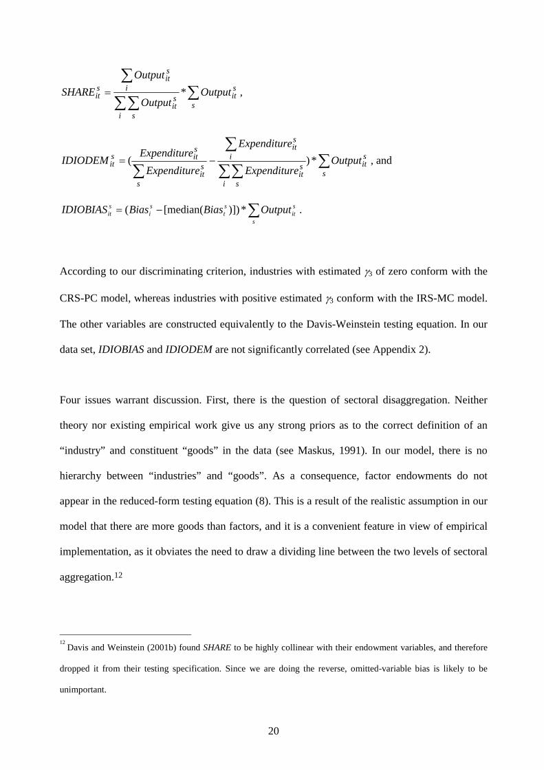
According to our discriminating criterion, industries with estimated �3 of zero conform with the

CRS-PC model, whereas industries with positive estimated �3 conform with the IRS-MC model.

The other variables are constructed equivalently to the Davis-Weinstein testing equation. In our

data set, IDIOBIAS and IDIODEM are not significantly correlated (see Appendix 2).

Four issues warrant discussion. First, there is the question of sectoral disaggregation. Neither

theory nor existing empirical work give us any strong priors as to the correct definition of an

“industry” and constituent “goods” in the data (see Maskus, 1991). In our model, there is no

hierarchy between “industries” and “goods”. As a consequence, factor endowments do not

appear in the reduced-form testing equation (8). This is a result of the realistic assumption in our

model that there are more goods than factors, and it is a convenient feature in view of empirical

implementation, as it obviates the need to draw a dividing line between the two levels of sectoral

aggregation.12

12 Davis and Weinstein (2001b) found SHARE to be highly collinear with their endowment variables, and therefore

dropped it from their testing specification. Since we are doing the reverse, omitted-variable bias is likely to be

unimportant.

21

Second, there may exist potential for simultaneity of expenditure and output, and therefore bias

in the estimates of �2. The use of input-output tables allows us to obviate to this problem. One

source of simultaneity could arise from the use of the same data source in the construction of

expenditure and output variables. If expenditure is constructed by subtracting net exports from

output, measurement error will simultaneously affect dependent and independent variables, and

thus bias estimated coefficients. This is why we draw our expenditure and output data from

input-output tables. As pointed out by Trionfetti (2001), input-output tables should be immune

from the simultaneity problem through measurement error, because output and expenditure data

(horizontal and vertical entries) are collected from independent sources of raw data. In addition,

simultaneity bias could arise if some sectoral expenditure represents demand for intermediate

inputs that are classified under the same sector heading. Our testing equation (8) implies the

assumption that expenditure shares are an exogenous determinant of output location, but this

assumption is rarely satisfied in the data. It is for this reason that we have chosen to compute net

expenditure per sector as well as gross expenditure, which is possible in input-output tables. The

definition of “net expenditure” should include expenditure from those sources that use the

industry’s output for final consumption, and exclude expenditure from those sources that use the

output as intermediate inputs. Net expenditure is therefore computed as expenditure on the

industry’s output by private households and by the public sector, excluding expenditure by the

industry itself and by all other manufacturing industries.13 We call IDIODEM1 the variable

computed from gross expenditure values and IDIODEM2 the variable computed from net

expenditure values.

13 Specifically, net expenditure is calculated as the sum of the following four expenditure headings in the input-

output tables (NACE-Clio R44 codes in brackets): “final consumption of households on the economic territory”

(01), “general public services” (810), non-market services of education and research (850), and non-market services

of health (890).

22

Third, situ is likely to be heteroskedastic, as the variance of errors may well be positively

correlated with the size of countries.14 Our significance tests are therefore based on White-

corrected standard errors. We make this conservative adjustment in order to minimise the risk of

wrongly attributing sectors to the IRS-MC paradigm due to underestimation of the standard error

of �3.

Fourth, IDIODEM is a generated regressor, which could lead to bias in the coefficient estimates

on it and on all other explanatory variables (Pagan, 1980). No unbiased or consistent estimator

has as yet been derived analytically for the situation where an estimated coefficient of one

equation enters as an explanatory variable in another. We therefore resort to bootstrap

techniques. Resampling the data 5,000 times with replication, we re-estimated the coefficient

vectors and standard errors for each model. The difference between the original regression

coefficients and their bootstrap equivalents is a measure of estimation bias. We followed Efron’s

(1982) rule that bias is only a serious concern when the estimated bias is larger than 25 percent

of the standard error. It turned out that the estimated biases were significantly below that

threshold in all of the specifications that we estimated. Hence, we report the original coefficient

estimates together with original as well as bootstrap estimated standard errors.15

14 A Cook-Weisberg heteroskedasticity test on the pooled model strongly rejects the null of constant error variance.

15 One might think that the average estimated bootstrap coefficient is superior to the original regression estimate.

However, the bootstrap coefficient estimates have an indeterminate amount of random error and may thus have

greater mean square error than the (potentially biased) original regression estimates (Mooney and Duval, 1993). We

therefore report the original regression estimates.

23

4.3 Results

We first ran our model on the full data sample. The results are given in Table 5. In specification

(1), we use OLS to estimate the specification based on gross expenditure values (IDIODEM1).

This yields a coefficient on IDIOBIAS that is positive but not significantly different from zero,

hence we would infer that on the whole the CRS-PC model dominates the IRS-MC model. In

specification (2) we re-ran the same equation with IDIODEM2, which is based on net

expenditure values. We find that the coefficient on IDIODEM2 is significantly smaller than

IDIODEM1, the two coefficients being 0.60 and 1.17 respectively. This is confirms that the

coefficient on demand idiosyncrasies is biased upward if demand is measured in gross terms. We

also find that the estimated coefficient on IDIOBIAS is larger in the second specification and has

become statistically significantly different from zero. This suggests that, on average, the IRS-MC

model has stronger explanatory power than the CRS-PC model. Specifications (3) and (4), where

we account for observed heteroskedasticity across sectors and countries by estimating a panel

GLS model, confirm this result: the coefficient on IDIOBIAS, corresponding to c2 of our testing

equation (8) is always statistically significantly positive.

We know a priori that pooled runs impose too much structure, since our motivating hypothesis is

to find different parameter estimates for individual industries. The results of industry-by-industry

regressions are given in Table 6. The equation generally performs well, yielding R2s in the range

0.56 to 0.99. Coefficient estimates on IDIOBIAS are in the expected positive or insignificant

range for all industries.

At the 95-percent confidence level we find that, of the 18 industries, five conform with the IRS-

MC paradigm. The allocation of sectors looks broadly plausible.

24

It is interesting to measure the relative importance of the two paradigms in terms of their share of

industrial output (Table 6, columns 5/6). According to our results based on the six largest EU

economies, IRS-MC sectors account for around one quarter of industrial production. This share

was increasing over our sample period. The combined output share of the five IRS sectors in our

data set was 24.7 percent in 1970 and 26.7 percent in 1985.

A final comment is in order. Our estimates of the parameter �2 are consistent with those of Davis

and Weinstein (1996), namely, we do not find evidence of the magnification effect. Our

interpretation is different however. We do not interpret the absence of magnification effects as

validation of the CRS-PC paradigm, because, as discussed in the theory section, �2 may be

smaller than one in both CRS-PC and IRS-MC sectors when demand is home biased. According

to our model, �2 will take positive values, and will reflect important trade costs if it is

significantly larger than zero. Our results are consistent with this prediction. The estimated

coefficients on IDIODEM are never significantly negative, but they are significantly positive in

ten of our 18 sectors. This is another indication that the empirical testing equation, which is tied

closely to the underlying theoretical model, performs well in our data set.

25

5. Conclusions

We have developed and applied an empirical test to separate two paradigms of international

trade theory: a model with constant returns and perfect competition (CRS-PC), and a model with

increasing returns a monopolistic competition (IRS-MC). The discriminating criterion makes use

of the assumption that demand is home biased, an assumption that is strongly supported in the

empirical literature. We show theoretically that specialisation patterns are affected by inter-

country differences in the degree of home bias if an industry conforms to the IRS-MC paradigm,

but not if it is characterised by CRS-PC. This result provides us with a discriminating criterion

that we implement empirically. In the empirical part we estimate industry- and country-level

home biases through disaggregated gravity regressions, and use these estimates to apply our test

to a data set with 18 industries for the six major EU countries in 1970-85. The results suggest

that five industries, accounting for around a quarter of industrial output, can be associated with

IRS-MC.

In addition to the assumption that demand is home biased, our study distinguishes itself from the

literature on home-market effects in two principal ways. One feature is that the discriminating

criterion holds regardless of whether trade costs exist, and regardless of whether they exist only

in the IRS-MC sector or in both. This is a welcome feature especially in the light of the

sensitivity, highlighted in the recent literature, of the magnification effect to the way trade costs

appear in the model. Another innovation is that, in the empirical part, we draw on input-output

data. This allows us to relate production to final expenditure, and hence to avoid simultaneity

problems that might arise from regressing production on total expenditure where there are intra-

sectoral input-output linkages.

26

Bibliography

Anderson, James E. and Marcouiller, Douglas (2000) “Insecurity and the Pattern of Trade: An

Empirical Investigation”. Boston College Working Papers in Economics, No. 418.

Bergstrand, Jeffrey H. (1990) “The Heckscher-Ohlin-Samuelson Model, the Linder Hypothesis

and the Determinants of Bilateral Intra-Industry Trade”. Economic Journal, vol. 100, pp.

1216-1229.

Davis, Donald R. (1995) “Intraindustry Trade: A Heckscher-Ohlin-Ricardo Approach”. Journal

of International Economics, vol. 39, pp. 201-226.

Davis, Donald R. (1998) “The Home Market, Trade and Industrial Structure”. American

Economic Review, vol. 88, pp. 1264-.

Davis, Donald R. and Weinstein, David E. (1999) “Economic Geography and Regional

Production Structure: An Empirical Investigation”. European Economic Review, vol. 43, pp.

379-407.

Davis, Donald R. and Weinstein, David E. (2001a) “An Account of Global Factor Trade”.

American Economic Review, forthcoming.

Davis, Donald R. and Weinstein, David E. (2001b) “Market Access, Economic Geography and

Comparative Advantage: An Empirical Assessment”. Journal of International Economics,

forthcoming.

Deardorff, Alan V. (1998) “Determinants of Bilateral Trade: Does Gravity Work in a

Neoclassical World?” In: Frankel, Jeffrey A. (ed.) The Regionalization of the World

Economy, University of Chicago Press and NBER.

Efron, Bradley (1982) The Jackknife, the Bootstrap and Other Resampling Plans. Society for

Industrial and Applied Mathematics, Philadelphia.

27

Evans, Carolyn (2000) “The Economic Significance of National Borders”. Mimeo, Federal

Reserve Bank of New York.

Evenett, Simon J. and Keller, Wolfgang (2001) “On Theories Explaining the Success of the

Gravity Equation”. Journal of Political Economy, forthcoming.

Falvey, Rodney E. and Kierzkowski, Henryk (1987) “Product Quality, Intra-Industry Trade and

(Im)perfect Competition”. In: Kierzkowski, H. (ed.) Protection and Competition in

International Trade, Oxford University Press, pp. 143-161.

Feenstra, Robert C., Lipsey, Robert E. and Bowen, Harry P. (1997) “World Trade Flows, 1970-

1992, With Production and Tariff Data”. NBER Working Papers, No. 5910.

Feenstra, Robert C., Markusen, James A. and Rose, Andrew K. (2001) “Using the Gravity

Equation to Differentiate Among Alternative Theories of Trade”. Canadian Journal of

Economics, vol. 34, pp. p 430-47.

Greenaway, David and Milner, Chris (1986) The Economics of Intra-Industry Trade. Oxford,

Basil Blackwell.

Harrigan, James (1993) “OECD Imports and Trade Barriers in 1983”, Journal of International

Economics, vol. 35, pp. 95-111.

Haveman, Jon D. and Hummels, David (1997) “Gravity, What is it good for? Theory and

Evidence on Bilateral Trade”. Mimeo, Purdue University, W. Lafayette (IN).

Head, Keith and Mayer, Thierry (2000) “Non-Europe: The Magnitude and Causes of Market

Fragmentation in the EU”. Weltwirtschaftliches Archiv, vol. 136, pp. 284-314.

Head, Keith; Mayer, Thierry and Ries, John (2001) “On the Pervasiveness of Home Market

Effects”. Economica, forthcoming.

Head, Keith and Ries, John (2001) “Increasing Returns Versus National Product Differentiation

as an Explanation for the Pattern of US-Canada Trade”. American Economic Review,

forthcoming.

28

Helliwell, John F. (1996), “Do national borders matter for Quebec’s trade?”, Canadian Journal

of Economics, 29(3), pp. 507-22.

Helliwell, John F. (1997) “National Borders, Trade and Migration”. Pacific Economic Review,

vol. 3, pp. 165-185.

Helpman, Elhanan (1987), “Imperfect competition and international trade: evidence from

fourteen industrial countries”, Journal of the Japanese and International Economics, vol. 1,

pp. 62-81.

Hummels, David and Levinsohn, James (1995) “Monopolistic Competition and International

Trade: Reconsidering the Evidence”. Quarterly Journal of Economics, vol. 110, pp. 799-836.

Helpman, Elhanan and Krugman, Paul (1985) Market Structure and Foreign Trade. Cambridge

(Mass.), MIT Press.

Keeble, David; Offord, John and Walker, Sheila (1986) Peripheral Regions in a Community of

Twelve Member States. Commission of the European Communities, Luxembourg.

Krugman, Paul (1980) “Scale Economies, Product Differentiation, and the Pattern of Trade”.

American Economic Review, vol. 70, pp. 950-959.

Leamer, Edward E. (1997) “Access to Western Markets and Eastern Effort Levels”. In: Zecchini,

S. (ed.) Lessons from the Economic Transition. Kluwer, Boston.

Leamer, Edward E. and Levinsohn, James (1995) “International Trade Theory: The Evidence”.

In: Grossman, G. and Rogoff, K. (eds.) Handbook of International Economics, vol. 3,

Elsevier, New York.

Maskus, Keith (1991), “Comparing International Trade Data and Product and National

Characteristics Data for the Analysis of Trade Models”. In: Hooper, P. and Richardson, J.D.

(eds) International Economic Transactions: Issues in Measurement and Empirical Research,

University of Chicago Press, pp. 17-56.

29

McCallum, John (1995) “National Borders Matter: Canada-U.S. Regional Trade Patterns”.

American Economic Review, vol. 85, pp. 615-623.

Miyagiwa, Kaz (1991) “Oligopoly and Discriminatory Government Procurement Policy”.

American Economic Review, vol. 81, pp. 1321-1328.

Mooney, Christopher Z. and Duval, Robert D. (1993) Bootstrapping: A Nonparametric

Approach to Statistical Inference. Sage, Newbury Park (CA).

OECD (1999) Technical Note on OECD National Accounts. Organisation for Economic Co-

operation and Development, Paris. (http://www.oecd.org/std/natechn.htm)

Pagan, Adrian (1980) “Econometric Issues in the Analysis of Regressions with Generated

Regressors”. International Economic Review, vol. 25, pp. 221-247.

Polak, Jacques (1996) “Is APEC a Natural Regional Trading Bloc?” World Economy, vol. 19,

pp. 533-543.

Rauch, James E. (1999) “Networks Versus Markets in International Trade”. Journal of

International Economics, vol. 47, pp. 317-345.

Sachs, Jeffrey D. and Warner, Andrew M. (1995) “Economic Reform and the Process of Global

Integration”. Brookings Papers on Economic Activity, vol. 1, pp. 1-118.

Trefler, Daniel (1995) “The Case of Missing Trade and Other Mysteries”. American Economic

Review, vol. 85, pp. 1029-1046.

Trionfetti, Federico (2001) “Using Home-Biased Demand to Test for Trade Theories.”

Weltwirtschaftliches Archiv, vol. 137, pp. 404-426.

Wei, Shang-Jin (1996) “How Reluctant are Nations in Global Integration?” NBER Working

Paper, No. 5531.

Winters, Alan (1984) “Separability and the Specification of Foreign Trade Functions”. Journal

of International Economics, vol. 17, pp. 239-263.

30

TABLE 1: Interpretation of Parameter Values in the Testing Equation

c1 c2 Paradigm Trade costs

+ + IRS-MC � < 1

0 + IRS-MC � = 1

+ 0 CRS-PC � < 1

0 0 CRS-PC � = 1

31

TABLE 2: Gravity Equations: Full Sample (6 importing countries, 22 exporting countries, 18 sectors, 1970-85: dependent variable = log of

imports; beta coefficients in brackets)

OLS Tobit (1) (2) (3) (4) (5) HOMEDUM 0.64

(0.04) 1.54

(0.13) 0.54

(0.04) 1.81

(0.12) -0.25

(-0.02) LOGGDPH 1.33

(0.16) 2.78

(0.35) 1.33

(0.18) 1.33

(0.18) 1.33

(0.18) LOGGDPF 1.63

(0.26) -0.09# (-0.01)

1.63 (0.30)

1.63 (0.30)

1.63 (0.30)

LOGPOPH 0.68 (0.14)

0.72 (0.17)

0.70 (0.17)

0.70 (0.17)

0.70 (0.17)

LOGPOPF 0.56 (0.17)

0.28 (0.10)

0.57 (0.20)

0.57 (0.20)

0.57 (0.20)

LOGDIST -1.14 (-0.43)

-0.69 (-0.33)

-1.15 (-0.49)

LOGDIST1 -1.15 (-0.45)

LOGDIST2 -1.15 (-0.52)

LOGREMOTE 0.04 (0.25)

0.04 (0.27)

0.04

(0.27) 0.04

(0.27) 0.04

(0.27) BORDUM 0.32

(0.04) 0.38

(0.05) 0.31

(0.04) 0.31

(0.04) 0.31

(0.04) LANGDUM 0.93

(0.09) 0.62

(0.07) 0.97

(0.10) 0.97

(0.10) 0.97

(0.10) PTADUM 0.72

(0.10) 0.99

(0.15) 0.72

(0.11) 0.72

(0.11) 0.72

(0.11) CLOSEDDUM -1.29

(-0.12) -1.39

(-0.15) -1.39

(-0.15) -1.39

(-0.15) NTB -2.53

(-0.21)

No. of observations 37,968 22,176 37,968 37,968 37,968 No. of censored obs. n.a. n.a. 1,526 1,526 1,526 R2 0.44 0.42 n.a. n.a. n.a.

Note: All coefficients pass the t test at the 0.01% level, except that marked by #.

32

TABLE 3: Estimated Home-Country Biases by Country, 1970-85

Country Mean coefficient on HOMEDUM

Standard deviation of coefficients on HOMEDUM

Belgium-Luxembourg 0.50 2.24 France 4.34 2.82

West Germany 3.29 1.45 Italy -0.79 1.16

Netherlands 1.11 2.90 United Kingdom 2.84 1.22

Note: Based on Tobit regression (specification (3) of Table 2) estimated separately for each of the 6 importing countries and 18 sample industries.

33

TABLE 4: Estimated Home-Country Biases by NACE Industry, 1970-85

NACE code: Industry Mean coefficient on HOMEDUM

Standard deviation of coefficients on HOMEDUM

1170: Chemicals 2.21 2.22

1190: Metal goods 1.15 1.39

1210: Machinery 1.69 1.36

1230: Office machines 0.71 4.22

1250: Electrical goods 1.90 2.14

1270: Motor vehicles -0.21 3.59

1290: Other transp. eq. 1.94 1.54

1310: Meat products 3.50 3.35

1330: Dairy products 2.70 2.43

1350: Other food 3.45 1.92

1370: Beverages 2.26 2.97

1390: Tobacco products 4.76 4.70

1410: Textiles, clothing 2.18 3.15

1430: Leather, footwear 1.84 2.64

1450: Timber, furniture 0.39 1.60

1470: Pulp, paper, printing 0.41 1.25

1490: Rubber, plastic 1.63 1.99

1510: Instrum. engineering and other manuf.

2.29 2.28

Note: Based on Tobit regression (specification (3) of Table 2) estimated separately for each of the 6 importing countries and 18 sample industries.

34

TA

BL

E 5

: P

oole

d E

stim

atio

n of

the

Dis

crim

inat

ing

Cri

teri

on

(Dep

ende

nt v

aria

ble

= O

utpu

t; 4

00 o

bser

vatio

ns)

O

LS

GL

S (p

anel

het

eros

keda

stic

ity)

(1

) (2

) (3

) (4

)

SH

AR

E

1.00

66

(0.0

15, 0

.00)

[0

.015

, 0.0

0]

1.00

86

(0.0

25, 0

.00)

[0

.026

, 0.0

0]

1.00

87

(0.0

11, 0

.00)

[0

.021

, 0.0

0]

0.99

21

(0.0

11, 0

.00)

[0

.016

, 0.0

0]

ID

IOD

EM

1 1.

1745

(0

.045

, 0.0

0)

[0.0

49, 0

.00]

ID

IOD

EM

2

0.60

4 (0

.058

, 0.0

0)

[0.0

58, 0

.00]

0.54

3 (0

.024

, 0.0

0)

[0.0

38, 0

.00]

0.51

2 (0

.036

, 0.0

0)

[0.0

39, 0

.00]

IDIO

BIA

S 0.

0002

(0

.000

17, 0

.19)

[0

.000

17, 0

.19]

0.00

05

(0.0

0020

, 0.0

1)

[0.0

0021

, 0.0

1]

0.00

05

(0.0

0011

, 0.0

0)

[0.0

0010

, 0.0

0]

0.00

06

(0.0

0024

, 0.0

1)

[0.0

0017

, 0.0

0]

No.

of

obse

rvat

ions

40

0 40

0 40

0 40

0

R2

0.98

0.

94

n.a.

n.

a.

Pane

ls (

no.)

N

one

Non

e Se

ctor

s (1

8)

Cou

ntri

es (

6)

N

otes

: Rou

nd b

rack

ets:

est

imat

ed s

tand

ard

erro

rs (

Whi

te c

orre

cted

for

OL

S m

odel

s) a

nd P

val

ues.

Squ

are

brac

kets

: Boo

tstr

appe

d st

anda

rd e

rror

s (5

000

repl

icat

ions

with

rep

lace

men

t) a

nd P

val

ues.

Con

stan

t ter

m in

clud

ed in

all

regr

essi

ons

but n

ot r

epor

ted

(nev

er s

tatis

tical

ly s

igni

fica

ntly

di

ffer

ent f

rom

zer

o).

35

TA

BL

E 6

: In

dust

ry-b

y-In

dust

ry E

stim

atio

n of

the

Dis

crim

inat

ing

Cri

teri

on

(OL

S, d

epen

dent

var

iabl

e =

Out

put;

boot

stra

pped

sta

ndar

d er

rors

bra

cket

s)

(1)

(2)

(3)

(4)

(5)

(6)

NA

CE

D

escr

ipti

on

SHA

RE

ID

IOD

EM

ID

IOB

IAS

R2

No.

of

obs.

P

ara-

digm

O

utpu

t sh

are

in 1

970

(%)

Out

put

shar

e in

198

5 (%

) 17

0 C

hem

ical

s 0.

95 (

0.06

)*

-0.1

5 (0

.30)

0.

0019

(0.0

017)

0.

98

23

CR

S 10

.0

12.9

190

Met

al g

oods

1.

18 (

0.06

)*

1.29

(0.

63)

-0.0

021

(0.0

062)

0.

98

23

CR

S 9.

8 8.

4

210

Mac

hine

ry

1.29

(0.

08)*

1.

63 (

1.03

) -0

.002

1 (0

.006

2)

0.95

23

C

RS

9.7

9.5

230

Off

ice

mac

hine

s 1.

05 (

0.06

)*

0.61

(0.

09)*

0.

0005

(0.0

002)

* 0.

99

19

IRS

2.0

2.7

250

Ele

ctri

cal g

oods

1.

16 (

0.10

)*

0.74

(0.

53)

0.00

05 (0

.003

4)

0.97

23

C

RS

8.4

8.8

270

Mot

or v

ehic

les

1.01

(0.

08)*

1.

03 (

0.22

)*

0.00

37 (0

.001

3)*

0.98

23

IR

S 7.

8 8.

4

290

Oth

er tr

ansp

. eq.

0.

80 (

0.15

)*

0.68

(0.

22)*

0.

0015

(0.0

035)

0.

82

23

CR

S 2.

5 3.

1

310

Mea

t pro

duct

s 0.

71 (

0.05

)*

0.42

(0.

04)*

0.

0014

(0.0

005)

* 0.

98

20

IRS

5.3

4.9

330

Dai

ry p

rodu

cts

0.80

(0.

05)*

0.

42 (

0.07

)*

0.00

21 (0

.000

4)*

0.97

23

IR

S 2.

8 3.

0

350

Oth

er f

ood

0.79

(0.

04)*

0.

34 (

0.26

) -0

.002

4 (0

.001

7)

0.97

23

C

RS

9.4

8.9

370

Bev

erag

es

0.97

(0.

07)*

0.

35 (

0.07

)*

0.00

003

(0.0

006)

0.

94

23

CR

S 3.

3 2.

4

390

Tob

acco

pro

duct

s 0.

97 (

0.04

)*

0.39

(0.

04)*

0.

0001

(0.0

002)

0.

98

23

CR

S 2.

4 1.

2

410

Tex

tiles

, clo

thin

g 0.

63 (

0.19

)*

1.21

(0.

56)

0.00

66 (0

.006

3)

0.82

23

C

RS

9.8

7.4

430

Lea

ther

, foo

twea

r 0.

74 (

0.20

)*

1.75

(0.

37)*

0.

0002

(0.0

010)

0.

85

23

CR

S 1.

6 1.

7

450

Tim

ber,

fur

nitu

re

1.06

(0.

08)*

0.

35 (

0.19

) -0

.004

3 (0

.001

8)

0.95

23

C

RS

4.3

3.7

470

Pulp

, pap

er, p

rint

ing

0.84

(0.

06)*

0.

27 (

0.21

) 0.

0070

(0.0

028)

* 0.

98

23

IRS

6.8

7.7

490

Rub

ber,

pla

stic

1.

12 (

0.03

)*

0.58

(0.

23)*

-0

.000

1 (0

.000

3)

0.99

23

C

RS

3.3

3.9

510

Inst

rum

. eng

inee

ring

and

oth

er

man

uf.

0.56

(0.

26)*

0.

39 (

0.15

)*

-0.0

004

(0.0

014)

0.

56

16

CR

S 1.

0 1.

4

Not

es: *

den

otes

sta

tist

ical

sig

nifi

canc

e at

the

95%

con

fide

nce

leve

l.

36

Appendix 1: Theoretical Extensions

A1.1 No Magnification Effect in IRS-MC Sectors When Demand is Home Biased We can show that the derivative �� dd / is not necessarily larger than one when demand is home

biased. Let us define the left-hand side of (7) as a � ���� ,,,, 21 hhP . Unfortunately, in general, the roots of this polynomial are long expression that are not manageable (even for the computer) except in the following two cases. Case A: Identical Countries

Setting 1�� and hhh �� 21 the only positive root of the polynomial is 1�� . Differentiating totally around this root gives:

� � � �� �

� �� � � �� � � � � �

1111

111

/.

/.,

22

22

���������

�����

��hh

hh

P

Ph

d

d

����

��

���

This derivative, although it is larger than one, i.e. it exhibits the magnification effect, is always smaller than the derivative under the benchmark case, which is:

� � � �� �

� �� � 11

1

/.

/.�

��

�����

����

��

���

P

P

d

d

Hence, home-biased demand attenuates the size of the magnification effect. Case B: Non-Identical Countries

In this example we drop the assumption of identical countries by assuming that only country 2 is home biased (i.e., 01 �h ) so that the polynomial � ���� ,,,, 21 hhP reduces to a second-degree polynomial. Differentiating around its only positive root gives:

� � � � � � � �� � � � �

� � � �� 212222

22

222

22

1

2222

22

1222

2111221,,

�����

��������������

�����

������������

��

hhhh

hhhhhhh

d

d

This expression is not particularly informative. Yet, after assigning specific values to one of the three parameters, the expression can be plotted in a three-dimensional space. An example is in

Figure A1, where the expression for � �2,, hd

d��

�� is compared with the constant 1. The figure

(computed at 1�� ) shows a large domain in which � � 1,1, 2 hd

d�

�� , i.e., no magnification effect

exists. Many other combinations of parameter values also yield no magnification effect.

37

0.20.4

0.60.8

1h2

0.30.4

0.50.6

0.70.8

0.91

�

012345

�� dd /

1

Figure A1.1: An Example of the Domain with No Magnification Effect A1.2 Home Bias in the CES Aggregate The home bias may be modelled in the utility function also at the CES sub-utility level, for instance in the following way.

� � � �111 �

�

�

�

�

���

���

��� ��

�

�

�

�

�

�

��ji nk

ijink

iikii ccu ,

where the weights � and � represent the bias. Then, defining iiih �� /� , the market equilibrium

equations (compacted into one) for the IRS-MC product becomes

02221

21

211

1 ���

���

XX Enhn

hE

nnh

h

��

��

,

and the derivative is

� � � �� �21112

2

32

2121

22

121,,,�����

������

��

hhhh

hhhhhhhh

d

d

���

����� ,

which is not necessarily larger than one, even at 1�� . Hence, the magnification effect cannot serve as a robust discrimination criterion here either.

38

A1.3. Trade Costs in the CRS-PC Sector In this section we show that home-biased demand is irrelevant for international specialisation in the CRS-PC sector even if these goods are traded at a transport cost. Introducing trade costs in the homogeneous goods results in the non-equalisation of factor prices. The major consequence for our paper is that we cannot derive equation (7) and the expression for dhd /� as neatly as we do under factor price equalisation. This notwithstanding, we can show the irrelevance of the home bias in CRS-PC sectors by inspection of the market equilibrium equations. For clarity of exposition we consider the situation where, say, country 1 is a net exporter of Y. Naturally, the choice of the country is irrelevant. Assume that for each unit of Y shipped, only a fraction

� �1,0�� arrives at destination. Then, equation (6) becomes

� �� � �� 22112222211111 11 YpYpEhEhpEhEhp YYYYYYYYYYYY �� �������

Once again, hYi cancels out of this expression. This means that the home bias is irrelevant for international specialisation in the CRS-PC sector and, therefore, that the assumption of free trade in Y and Z made in Section 3 is purely a matter of analytical convenience.

39

Appendix 2: Data Description

Output data are taken from input-output tables in Eurostat’s “National Accounts ESA” series. Bilateral trade data are taken from the World Trade Database, available through Feenstra et al. (1997). We retained trade data recorded by the importing countries. These data, original classified under SITC headings, were concorded with the NACE input-output data used for the output values. Hence, all trade flows are c.i.f., and our estimates of trade within countries can be considered conservative. Observations for which estimated intra-country trade was, implausibly, negative (i.e. Output-Exports<0) were set to zero. The following 22 exporting countries are contained in our sample: Australia, Austria, Belgium-Luxembourg, Canada, Denmark, Finland, France, Germany, Greece, Ireland, Italy, Japan, Netherlands, New Zealand, Norway, Portugal, Spain, Sweden, Turkey, UK, USA, Yugoslavia. A list of the 18 NACE industries in our data set can be found in Table 6. Distance data measure great circle distances between the countries’ capital cities. They are from Jon Haveman (www.macalester.edu/research/economics/PAGE/HAVEMAN/Trade.Resources/TradeData.html). Inclusion of a remoteness variable in the gravity model has been advocated persuasively by Polak (1996). LOGREMOTE is defined as follows (in the spirit of Helliwell, 1997):

]2[, ,, � �

���jik tkjkiktij LOGGDPLOGDISTLOGDISTLOGREMOTE .

The linguistic groupings underlying LANGDUM are defined as follows: English: Australia, Canada, Ireland, New Zealand, UK, USA; French: Belgium, Canada, France; German: Austria, Germany; Dutch: Belgium, Netherlands; Scandinavian: Denmark, Sweden, Norway. The preferential trade areas underlying PTADUM are defined as follows: EU: Belgium, Denmark (1973-), Greece (1981-), France, Germany, Ireland (1973-), Italy, UK (1973-). EFTA: Austria, Denmark (-1972), Norway, Portugal, Spain, Sweden, UK (-1972). Australia-New Zealand Free Trade Agreement: Australia, New Zealand. The dummy for trade “closedness” is from Sachs and Warner (1995). The dummy is set to zero if a country satisfies four tests: (1) average tariff rates below 40 percent; (2) average quota and licensing coverage of imports of less than 40 percent; (3) a black market exchange rate premium that averaged less than 20 percent during the 1970s and 1980s; and (4) no extreme controls (taxes, quotas, state monopolies) on exports. It turns out that this measure is time invariant in our data set. According to the Sachs-Warner criteria, New Zealand, Turkey and Yugoslavia were “closed” for the whole time interval 1970-85, whilst the remaining 19 countries were “open” throughout this period. Correlations among the variables of our testing equation (underlying Table 4, 9816 obs.): Output SHARE IDIODEM IDIOBIAS Output 1.000 SHARE 0.624 1.000 IDIODEM 0.219 -0.002 1.000 IDIOBIAS 0.287 0.364 -0.049 1.000