![Jean-Pierre Dupuy IMETIC THEORY AS SCIENCE+Mimetic+Theory.pdf · Jean-Pierre Dupuy 1. MIMETIC THEORY AS SCIENCE This paper is about Mimetic Theory [MT] and its efforts to constitute](https://static.fdocuments.net/doc/165x107/5e17950bec51206ecd3d09f1/jean-pierre-dupuy-imetic-theory-as-mimetictheorypdf-jean-pierre-dupuy-1-mimetic.jpg)
A SPECTRAL MIMETIC LEAST-SQUARES METHOD FOR THE … · A SPECTRAL MIMETIC LEAST-SQUARES METHOD FOR...
22
A SPECTRAL MIMETIC LEAST-SQUARES METHOD FOR THE STOKES EQUATIONS WITH NO-SLIP BOUNDARY CONDITION MARC GERRITSMA AND PAVEL BOCHEV Dedicated to Max Gunzburger’s 70th birthday. Abstract Formulation of locally conservative least-squares finite element methods (LS- FEM) for the Stokes equations with the no-slip boundary condition has been a long stand- ing problem. Existing LSFEMs that yield exactly divergence free velocities require non- standard boundary conditions [3], while methods that admit the no-slip condition satisfy the incompressibility equation only approximately [4, Chapter 7]. Here we address this problem by proving a new non-standard stability bound for the velocity-vorticity-pressure Stokes system augmented with a no-slip boundary condition. This bound gives rise to a norm-equivalent least-squares functional in which the velocity can be approximated by div-conforming finite element spaces, thereby enabling a locally-conservative approxima- tions of this variable. We also provide a practical realization of the new LSFEM using high-order spectral mimetic finite element spaces [15] and report several numerical tests, which confirm its mimetic properties. 1. Introduction In this paper we consider least-squares finite element methods (LSFEMs) for the velocity- vorticity-pressure (VVP) formulation of the Stokes problem (1) ∇× ω + ∇ p = f in Ω ∇× u - ω = 0 in Ω ∇· u = 0 in Ω , where u denotes the velocity, ω the vorticity, p the pressure and f the force per unit mass. Our main focus is on the formulation of conforming LSFEMs that are (i) locally conservative, and (ii) provably stable when the system (1) is augmented with the no-slip (velocity) boundary condition (2) u = 0 on ∂Ω. Note that (2) is equivalent to a pair of boundary conditions (3) u · n = 0 and u × n = 0 on ∂Ω , for the normal and tangential components of the velocity field, respectively. Formulation of conforming LSFEMs that satisfy both (i) and (ii) had been a long- standing challenge. Existing conforming methods generally fall into one of the following two categories. The LSFEMs in the first category, see e.g., [2], [8], are stable and ac- curate for (1) with the boundary condition (2) but satisfy ∇· u = 0 only approximately. Date: August 20, 2015. 1991 Mathematics Subject Classification. Primary 65N30, 65N35; Secondary 35J20, 35J46. Key words and phrases. Least-squares, mimetic methods, spectral element method, mass conservation. This paper is in final form and no version of it will be submitted for publication elsewhere. 1
Transcript of A SPECTRAL MIMETIC LEAST-SQUARES METHOD FOR THE … · A SPECTRAL MIMETIC LEAST-SQUARES METHOD FOR...
A SPECTRAL MIMETIC LEAST-SQUARES METHOD FOR THE STOKESEQUATIONS WITH NO-SLIP BOUNDARY CONDITION
MARC GERRITSMA AND PAVEL BOCHEV
Dedicated to Max Gunzburger’s 70th birthday.
Abstract Formulation of locally conservative least-squares finite element methods (LS-FEM) for the Stokes equations with the no-slip boundary condition has been a long stand-ing problem. Existing LSFEMs that yield exactly divergence free velocities require non-standard boundary conditions [3], while methods that admit the no-slip condition satisfythe incompressibility equation only approximately [4, Chapter 7]. Here we address thisproblem by proving a new non-standard stability bound for the velocity-vorticity-pressureStokes system augmented with a no-slip boundary condition. This bound gives rise toa norm-equivalent least-squares functional in which the velocity can be approximated bydiv-conforming finite element spaces, thereby enabling a locally-conservative approxima-tions of this variable. We also provide a practical realization of the new LSFEM usinghigh-order spectral mimetic finite element spaces [15] and report several numerical tests,which confirm its mimetic properties.
1. Introduction
In this paper we consider least-squares finite element methods (LSFEMs) for the velocity-vorticity-pressure (VVP) formulation of the Stokes problem
(1)
∇ × ω + ∇p = f in Ω
∇ × u − ω = 0 in Ω
∇ · u = 0 in Ω
,
where u denotes the velocity, ω the vorticity, p the pressure and f the force per unitmass. Our main focus is on the formulation of conforming LSFEMs that are (i) locallyconservative, and (ii) provably stable when the system (1) is augmented with the no-slip(velocity) boundary condition
(2) u = 0 on ∂Ω.
Note that (2) is equivalent to a pair of boundary conditions
(3) u · n = 0 and u × n = 0 on ∂Ω ,
for the normal and tangential components of the velocity field, respectively.Formulation of conforming LSFEMs that satisfy both (i) and (ii) had been a long-
standing challenge. Existing conforming methods generally fall into one of the followingtwo categories. The LSFEMs in the first category, see e.g., [2], [8], are stable and ac-curate for (1) with the boundary condition (2) but satisfy ∇ · u = 0 only approximately.
Date: August 20, 2015.1991 Mathematics Subject Classification. Primary 65N30, 65N35; Secondary 35J20, 35J46.Key words and phrases. Least-squares, mimetic methods, spectral element method, mass conservation.This paper is in final form and no version of it will be submitted for publication elsewhere.
1
2 MARC GERRITSMA AND PAVEL BOCHEV
Conversely, the LSFEMs in the second category; see, e.g., [3], [4, Chapter 7] yield exactlydivergence free velocity fields but require the non-standard normal velocity, tangential vor-ticity boundary condition
(4) u · n = 0 and ω × n = 0 on ∂Ω ,
i.e., they specify only the first of the two velocity conditions in (3).Thus far, achieving both stability and mass conservation with the velocity boundary
condition has been only possible by switching to a non-conforming formulations such asthe discontinuous LSFEMs in [6] and [7]. In this paper we address this problem by de-veloping a new, non-standard a priory stability bound for the VVP Stokes system with (2).We refer to this bound as “non-standard” because (i) it uses an operator norm to measurethe residual of the momentum equation in (1), instead of a conventional Sobolev spacenorm, and (ii) it employes a weak curl and grad operator in the second equation of (1).This stability bound gives rise to a norm-equivalent functional, which can be discretizedby using div-conforming elements for the velocity fild. In so doing we are able to obtain aLSFEM that is both locally conservative and stable for (1)–(2).
We have organized the rest of the paper as follows. Section 2 introduces notation andsome necessary background results. In Section 3 a non-standard stability bound will begiven. In Section 4 the associated variational formulation will be presented. Section 5 in-troduces conforming finite dimensional subspaces which respect the properties of the exactsequences. In this section all operations on polynomials will be represented by operationson their expansion coefficients. Results of the mimetic least-squares spectral element willbe presented. Concluding remarks and future work are discussed in Section 7.
2. Preliminaries
In what follows Ω ⊂ Rd, d = 2, 3 is a bounded open region with Lipschitz boundary ∂Ω.We recall the space L2(Ω) of all square integrable functions with norm and inner productdenoted by ‖ · ‖0 and (·, ·)0, respectively, and its subspace L2
0(Ω) of all square integrablefunctions with a vanishing mean. The spaces H(grad,Ω), H(curl,Ω) and H(div,Ω) containsquare integrable functions whose gradient, curl and divergence are also square integrable.When equipped with the graph norms
‖q‖grad := ‖q‖20 + ‖∇q‖20, ‖ξ‖2curl := ‖ξ‖20 + ‖∇ × ξ‖20 , and ‖v‖2div := ‖v‖20 + ‖∇ · v‖20 ,
the spaces H(grad,Ω), H(curl,Ω) and H(div,Ω) are Hilbert spaces.We will also need the factor space H(grad,Ω)/R, which contains equivalence classes
of functions in H(grad,Ω) differing by a constant, and the subspaces
H0(curl,Ω) = v ∈ H(curl,Ω) |v × n = 0 on ∂Ω ,
H0(div,Ω) = v ∈ H(div,Ω) |v · n = 0 on ∂Ω ,
of H(curl,Ω) and H(div,Ω), respectively containing functions whose tangential and nor-mal traces vanish on the boundary. The Poincare inequalities
(5) ‖q‖0 ≤ C‖∇q‖0, ‖ξ‖0 ≤ C ‖∇ × ξ‖0 + ‖∇ · ξ‖0 , ‖v‖0 ≤ C ‖∇ · v‖0 + ‖∇ × v‖0 ,
which hold for all q ∈ H(grad,Ω)/R, ξ ∈ H0(curl,Ω) and v ∈ H0(div,Ω), respectively,imply that the associated semi-norms are norms on these spaces.
The spaces H(grad,Ω), H(curl,Ω) and H(div,Ω), and the associated spaces H(grad,Ω)/R,H0(curl,Ω), and H0(div,Ω) provide the domains for the gradient, divergence and curl oper-ators. We denote the ranges of these operators byR(?), resp., R0(?) where? ∈ ∇,∇×,∇·.For instance, R(∇×) is the range of curl acting on H(curl,Ω) and R0(∇·) is the range of
MIMETIC LSFEM FOR THE STOKES EQUATIONS 3
divergence acting on H0(div,Ω). Likewise, N(?), resp. N0(?) are the nullspaces of theseoperators in the appropriate function spaces.
The vector identities ∇ × (∇) = 0 and ∇ · (∇×) ≡ 0 imply that R0(∇) ⊆ N0(∇×),R0(∇×) ⊆ N0(∇·), and R(∇) ⊆ N(∇×) and R(∇×) ⊆ N(∇·). In this paper we assume thatΩ is such that
(6) R0(∇) = N0(∇×), R(∇) = N(∇×) and R0(∇×) = N0(∇·), R(∇×) = N(∇·).
A sufficient condition1 for (6) to hold is for Ω to be a contractible, or star-shaped. Thisresult is known as general Poincare lemma [19, p.69]
2.1. Adjoint operators and decompositions. The proof of the non-standard stabilitybound in Section 3 uses on orthogonal decompositions of H0(div,Ω) and H(div,Ω). SinceR0(∇×) is a closed subspace of H0(div,Ω) and R(∇×) is a closed subspace of H(div,Ω),assumption (6) implies that
H0(div,Ω) = R0(∇×) ⊕ R0(∇×)⊥ = N0(∇·) ⊕ N0(∇·)⊥
H(div,Ω) = R(∇×) ⊕ R(∇×)⊥ = N(∇·) ⊕ N(∇·)⊥ .For instance, the first decomposition means that every u ∈ H0(div,Ω) can be written as
(7) u = uN + uN⊥ .
where uN ∈ N0(∇·) and uN⊥ ∈ N(∇·)⊥. The nullspace component uN = ∇ × ξ solves thevariational equation: seek ξ ∈ H0(curl,Ω) and µ ∈ H0(grad,Ω) such that
(8)(∇ × ξ,∇ × ζ)0 + (ζ,∇µ)0 = (u,∇ × ζ)0 ∀ζ ∈ H0(curl,Ω),
(ξ,∇λ)0 = 0 ∀λ ∈ H0(grad,Ω)
The orthogonal complement component uN⊥ solves a similar mixed problem: seek uN⊥ ∈
H0(div,Ω) and φ ∈ L20(Ω) such that
(9)(uN⊥ ,v)0 + (φ,∇ · v)0 = 0 ∀v ∈ H0(div,Ω),
(∇ · uN⊥ , ϕ)0 = (∇ · u, ϕ) ∀ϕ ∈ L20(Ω)
For a given φ ∈ L20(Ω) the first equation in (9) induces a mapping φ 7→ uN⊥ which we call
a “weak” gradient ∇∗ of φ. Succinctly, ∇∗ : L20(Ω) 7→ H0(div,Ω) according to
(10) (∇∗φ,v)0 := (φ,−∇ · v)0 , ∀v ∈ H0(div,Ω) .
One can show that under assumption (6) there holds N0(∇·)⊥ = R0(∇∗) and so,
(11) H0(div,Ω) = R0(∇×) ⊕ R0(∇∗) .
In other words, the decomposition assumes the form
(12) u = ∇ × ξ + ∇∗φ
where ξ ∈ H0(curl,Ω) and φ ∈ L20(Ω). In particular, φ ∈ L2
0(Ω) satisfies ∇∗φ · n = 0.We will also need a “weak” version of the curl operator ∇∗×u : H(div,Ω) 7→ H(curl,Ω)
defined by
(13) (∇∗ × u, ξ)0 := (u,∇ × ξ)0 , ∀ξ ∈ H(curl,Ω) .
The operator ∇∗× enforces weakly the boundary condition u × n = 0 on its argument.And we need a “weak” version of the gradient operator ∇∗p : L2(Ω) 7→ H(div,Ω)
defined by
(14) (∇∗p,u)0 := (p,−∇ · u)0 , ∀u ∈ H(div,Ω) .
1The first identity holds if Ω has no loops, whereas the second identity holds if Ω has no holes.
4 MARC GERRITSMA AND PAVEL BOCHEV
2.2. Weak norms and seminorms. The a priory stability bound for (1) that providesthe foundation for our mimetic LSFEM requires nonstandard norms and seminorms forfunctions in H(div,Ω), H(curl,Ω) and L2(Ω). First, for any u ∈ H(div,Ω) we define
(15) ‖u‖D = supv∈H(div,Ω)
(u,v)0
‖v‖div.
Second, for any ξ ∈ H(curl,Ω) we define
(16) ‖∇ × ω‖N0 := supv∈N0(∇·)
(∇ × ω,v)0
‖v‖div.
Lastly, for any p ∈ L2(Ω) we define
(17) ‖∇∗p‖N⊥0 := supv∈N0(∇·)⊥
(p,∇ · v)0
‖v‖div.
Norm (15) is simply the norm on the dual space H(div,Ω)′. Insofar as (16) is concernedtaking sup over the nullspace N0(∇·) implies that
‖∇ × ω‖N0 ≤ ‖∇ × ω‖0
and so we call (16) weak curl semi norm. Finally, it is easy to see that (17) satisfies
‖∇∗p‖N⊥0 ≤ ‖∇∗p‖0
and we will refer to it as the weak norm on L2(Ω).
3. Non-standard stability bound
In this section we establishes a priori stability bound for the VVP Stokes system (1)with the no-slip boundary condition (3). The proof draws upon the techniques in [3] withone important distinction. Stability proof in that paper relies on the orthogonality between∇ × ω and ∇∗p when ω has a vanishing tangential component, i.e., the fact that
(18) (∇ × ω,∇∗p) = 0 ∀ω ∈ H0(curl,Ω) and p ∈ L2(Ω) .
This implies a trivial lower bound (in fact an identity) for the L2-norm of the residual ofthe momentum equation
(19) ‖∇ × ω + ∇∗p‖0 ≥ ‖∇ × ω‖0 + ‖∇∗p‖0 ,
which represents a key juncture in the proof.However, for the case of the no-slip boundary condition of interest to us,ω ∈ H(curl,Ω)
and ∇ × ω is not orthogonal to ∇∗p. As a result, (18), resp. (19) do not hold. Nonetheless,the following theorem demonstrates that a lower bound similar to (19) can be establishedin terms of appropriate weak norms and semi norms.
Theorem 1. For all ω ∈ H(curl,Ω) and all p ∈ L2(Ω) there holds
(20) ‖∇ × ω + ∇∗p‖D ≥12
(‖∇ × ω‖N0 + ‖∇∗p‖N⊥
).
Proof. In order to bound the dual norm (15) from below by the weak curl-seminorm werestrict the supremum to functions in N0(∇·) and use the fact that ∇∗p ∈ N⊥0 (∇·), see (14).As a result,
‖∇ × ω + ∇∗p‖D = supv∈H(div,Ω)
(∇ × ω + ∇∗p,v)0
‖v‖div≥ supv∈N0(∇·)
(∇ × ω + ∇∗p,v)0
‖v‖div
∇∗p∈N⊥0 (∇·)= sup
v∈N0(∇·)
(∇ × ω,v)0
‖v‖div= ‖∇ × ω‖N0 .(21)

MIMETIC LSFEM FOR THE STOKES EQUATIONS 5
Similarly, to bound the dual norm in terms of the weak L2 norm we restrict the supremumto the orthogonal complement N0(∇·)⊥. From (12) we know that all elements of N0(∇·)⊥
are given by ∇∗φ for φ ∈ L20(Ω). From (13) we have that
0 = (∇∗ × ∇∗φ,ω)0 = (∇∗φ,∇ × ω)0 ,
where again ∇∗× weakly enforces ∇∗φ × n = 0:
‖∇ × ω + ∇∗p‖D = supv∈H(div,Ω)
(∇ × ω + ∇∗p,v)0
‖v‖div≥ supv∈N0(∇·)⊥
(∇ × ω + ∇∗p,v)0
‖vp‖div
∇×ω⊥N0(∇·)⊥= sup
v∈N0(∇·)⊥
(∇∗p,v)0
‖v‖div= ‖∇∗p‖N⊥0 .(22)
Combination of these two bounds proves the theorem:
‖∇ × ω + ∇∗p‖D =12‖∇ × ω + ∇∗p‖D +
12‖∇ × ω + ∇∗p‖D
(21,22)≥
12‖∇ × ω‖N0 +
12‖∇∗p‖N⊥ .(23)
Remark 1. Unlike the case of the nonstandard normal velocity-tangential vorticity bound-ary condition considered in [3], in which (19) holds with an identity, Theorem 1 can onlybound a dual norm of the momentum equation from below by weaker semi norms of thevorticity and the pressure. As mentioned at the beginning of this section, the reason for thisis the lack of orthogonality between ∇ × ω and ∇∗p.
To state the main result of this section it is convenient to introduce the “weak” curl norm
‖ω‖2N0= ‖ω‖20 + ‖∇ × ω‖2N0
.
Theorem 2. There exists a constant C > 0 such that
‖∇ × ω + ∇∗p‖2D + ‖ω − ∇∗ × u‖20 + ‖∇ · u‖20 ≥ C‖ω‖2N0
+ ‖u‖div + ‖∇∗p‖2N⊥0
.
for every ω ∈ H(curl,Ω), u ∈ H0(div,Ω) and p ∈ L2(Ω).
Proof. The proof follows the ideas in [3]. We have
(24) ‖∇∗ × u − ω‖20 = ‖∇∗ × u‖20 + ‖ω‖20 − 2(∇∗ × u, ω)
where ∇∗× is the weak curl2 defined in (13). To bound the last term we split it in two equalparts. On the one hand, the Cauchy-Schwartz inequality gives the bound
(∇∗ × u, ω) ≤ ‖∇∗ × u‖0‖ω‖0 .
On the other hand, using (12) and (13)
(∇∗ × u,ω) = (∇∗ × (uN + uN⊥ ),ω) = (∇∗ × uN ,ω) = (uN ,∇ × ω) ,
and since uN ∈ N0(∇·) definition (16) of the weak curl semi norm implies
(uN ,∇ × ω) ≤ ‖uN‖0‖∇ × ω‖N0 ≤ ‖u‖0‖∇ × ω‖N0 .
Using these inequalities in (24) gives the bound
‖∇∗ × u − ω‖20 ≥ ‖∇∗ × u‖20 + ‖ω‖20 − ‖∇
∗ × u‖0‖ω‖0 − ‖u‖0‖∇ × ω‖N0 .
2We recall that this operator enforces u × n = 0 in a weak, variational sense. As a result, the first part ofthe no-slip condition (3) is enforced strongly through u ∈ H0(div,Ω), while the second part is enforced weaklythrough the definition of ∇∗×.
6 MARC GERRITSMA AND PAVEL BOCHEV
Using the ε-inequality for the last two terms gives
‖∇∗ × u − ω‖20
≥
(1 −
δ
2
)‖∇∗ × u‖20 +
(1 −
12δ
)‖ω‖20 −
ε
2‖u‖20 −
12ε‖∇ × ω‖2N0
.(25)
Using Poincare-Friedrichs inequality [4, Theorems A.10-A.11]
(26) ‖∇∗ × u‖20 + ‖∇ · u‖20 ≥1
C2P
‖u‖20 ,
gives
‖∇∗ × u − ω‖20 + ‖∇ · u‖20 ≥12
(1 − δ) ‖∇∗ × u‖20 +12‖∇ · u‖20
+
(1 −
12δ
)‖ω‖20 +
12
1C2
P
− ε
‖u‖20 − 12ε‖∇ × ω‖2N0
.(27)
Adding β times the momentum equation yields and using Theorem 1
β‖∇ × ω+∇∗p‖2D + ‖∇∗ × u − ω‖20 + ‖∇ · u‖20
≥12
(1 − δ) ‖∇∗ × u‖20 +12‖∇ · u‖20 +
(1 −
12δ
)‖ω‖20+
12
1C2
P
− ε
‖u‖20 +12
(β − ε) ‖∇ × ω‖2N0+β
2‖∇∗p‖2N⊥0 .(28)
For the specific choice ε = 1/C2P, δ = 2/3 and β = 1 + 1/C2
P
(1 +1
C2P
)‖∇ × ω + ∇∗p‖2D + ‖∇∗ × u − ω‖20 + ‖∇ · u‖20
≥16‖∇∗ × u‖20 +
12‖∇ · u‖20 +
14‖ω‖20 +
12‖∇ × ω‖2N0
+1
2C2P
(C2P + 1)‖∇∗p‖2N⊥0(29)
≥ min1
6,
12C2
P
(C2P + 1)
(‖ω‖2curl + ‖u‖2H0(div,Ω) + ‖∇∗p‖2N⊥0
).
The theorem follows from
‖ω − ∇∗ × u‖20 + ‖∇ × ω + ∇∗p‖2D + ‖∇ · u‖20
≥C2
P
1 + C2P
(1 +1
C2P
)‖∇ × ω + ∇∗p‖2D + ‖∇∗ × u − ω‖20 + ‖∇ · u‖20
.(30)
4. Variational formulation
Based on the coercivity result in Theorem 2 we define the following least-squares func-tion for (ξ,v, q) ∈ X = H(curl,Ω) × H0(div,Ω) × L2(Ω) and f ∈ H(div,Ω)
(31) J(ξ,v, q;f ) :=12
‖∇∗ × v − ξ‖20 + ‖∇ × ξ + ∇∗q − f‖2D + ‖∇ · v‖20
.
The unique solution (ω,u, p) of the Stokes problem is then given by
(32) (ω,u, p) = arg min(ξ,v,q)∈X
J(ξ,v, q;f ) .
MIMETIC LSFEM FOR THE STOKES EQUATIONS 7
From the definition of the operator norm (15) it follows that for u ∈ H(div,Ω), ‖u‖D = 0 iff(u,v)0 = 0 for all v ∈ H(div,Ω). Every v ∈ H(div,Ω) has a decomposition v = ∇×ξ+∇∗qwith ξ ∈ H(curl,Ω) and q ∈ L2(Ω), although this decomposition is not orthogonal
‖∇ × ω + ∇∗p − f‖D = 0 ⇐⇒ (∇ × ω + ∇∗p − f ,∇ × ξ + ∇∗q)0 = 0 ,
for all ξ ∈ H(curl,Ω) and q ∈ L2(Ω). Taking variations of ‖ω − ∇∗ × u‖20 gives
(ω − ∇∗ × u, ξ − ∇∗ × v)0 = 0 ,
for all ξ ∈ H(curl,Ω) and v ∈ H0(div,Ω). Finally, conservation of mass is satisfied if‖∇ · u‖20 = 0 which implies that
(∇ · u,∇ · v)0 = 0 ,
for all v ∈ H0(div,Ω). If we collect all these conditions for a minimizer we obtain
(33)
(∇ × ω + ∇∗p,∇ × ξ)0 + (ω − ∇∗ × u, ξ)0 = (f ,∇ × ξ)0 ∀ξ ∈ H(curl,Ω)
(∇∗ × u − ω,∇∗ × v)0 + (∇ · u,∇ · v)0 = 0 ∀v ∈ H0(div,Ω)
(∇ × ω + ∇∗p,∇∗q)0 = (f ,∇∗q)0 ∀q ∈ L2(Ω)
Using integration by parts, using (13) and (14), we have: Find (ω,u, p) ∈ X such that(34)
(∇ × ω,∇ × ξ)0 + (ω, ξ)0 − (u,∇ × ξ)0 = (f ,∇ × ξ)0 ∀ξ ∈ H(curl,Ω)
− (∇ × ω,v)0 + (∇∗ × u,∇∗ × v)0 + (∇ · u,∇ · v)0 = 0 ∀v ∈ H0(div,Ω)
(∇∗p,∇∗q)0 = (−∇ · f , q)0 ∀q ∈ L2(Ω)
The well-posedness result, Theorem 2, is inherited on conforming subspaces Ch ⊂
H(curl,Ω), Dh0 ⊂ H0(div,Ω) and S h ⊂ L2(Ω). The variational equation then becomes:
Find (ωh,uh, ph) ∈ Xh = Ch × Dh0 × S h such that
(35) (∇ × ωh,∇ × ξh
)0
+(ωh, ξh
)0−
(uh,∇ × ξh
)0
=(f ,∇ × ξh
)0
∀ξh ∈ Ch
−(∇ × ωh,vh
)0
+(∇∗ × uh,∇∗ × vh
)0
+(∇ · uh,∇ · vh
)0
= 0 ∀vh ∈ Dh0(
∇∗ph,∇∗qh)
0=
(−∇ · f , qh
)0
∀qh ∈ S h
The next section will be devoted to the construction of such finite dimensional conformingsubspaces.
5. Mimetic spectral element method
Mimetic methods aim to decompose partial differential operators in a purely topologicalpart and a metric dependent part. The advantage of the purely topological description is thatit is independent of the size or shape of the mesh or the order of the approximation. We callsuch relations exact. The orthogonal decomposition of Dh
0 into divergence-free vector fieldsand irrotational vector fields is fully represented by the topological part. Approximationtakes place in the metric dependent part. In this section we will present the spectral elementbasis functions which span the finite dimensional spaces Ch, Dh and S h.
Similar ideas can be found in Tonti, [20, 21], Bossavit, [10, 11], Desbrun et al., [13],Bochev and Hyman, [5], Lipnikov et al, [17], Seslija et al., [18], Bonelle and Ern, [9],Lemoine et al., [16], Kreeft et al., [15] and references therein.
8 MARC GERRITSMA AND PAVEL BOCHEV
5.1. One dimensional basis spectral basis functions. Consider the interval [−1, 1] ⊂ Rand the Legendre polynomials, LN(ξ) of degree N, ξ ∈ [−1, 1]. The (N + 1) roots, ξi, of thepolynomial (1− ξ2)L′N(ξ) satisfy −1 ≤ ξi ≤ 1. Here L′N(ξ) is the derivative of the Legendrepolynomial. The zeros are called the Gauss-Lobatto-Legendre (GLL) points. Let hi(ξ) bethe Lagrange polynomial through the GLL points such that
(36) hi(ξ j) =
1 if i = j
0 if i , ji, j = 0, . . .N .
The explicit form of the Lagrange polynomials in terms of the Legendre polynomials isgiven by
(37) hi(ξ) =(1 − ξ2)L′N(ξ)
N(N + 1)LN(ξi)(ξi − ξ).
Let f (ξ) be defined for ξ ∈ [−1, 1] by
(38) f (ξ) =
N∑i=0
aihi(ξ) .
Using property (36) we see that f (ξ j) = a j, so the expansion coefficients in (38) coincidewith the value of f in the GLL nodes. We will refer to this expansion as a nodal expansion.The basis functions hi(ξ) are polynomials of degree N.
From the nodal basis functions we define the functions ei(ξ) by
(39) ei(ξ) = −
i−1∑k=0
dhk(ξ)dξ
dξ = −
i−1∑k=0
dhk(ξ) .
The functions ei(ξ) are polynomials of degree (N − 1). These polynomials satisfy, [14, 15]
(40)∫ ξ j
ξ j−1
ei(ξ) =
1 if i = j
0 if i , ji, j = 1, . . .N .
Let a function f (ξ) be expanded in these functions
(41) f (ξ) =
N∑i=1
biei(ξ) ,
then using (40) ∫ ξ j
ξ j−1
f (ξ) = b j .
So the expansion coefficients bi coincide with the integral of f over the edge [ξi−1, ξi]. Wewill call these basis functions edge functions and refer to the expansion (41) as an edgeexpansion, see for instance [1, 15] for examples of nodal and edge expansions.
Let f (ξ) be expanded in terms Lagrange polynomials as in (38), then the derivative of fis given by, [14, 15]
(42) f ′(ξ) =
N∑i=0
aih′i(ξ) =
N∑i=1
(ai − ai−1)ei(ξ) .
Remark 2. Note that the set of polynomials h′i, i = 0, . . . ,N is linear dependent andtherefore does not form a basis, while the set ei, i = 1, . . . ,N is linear independent andtherefore forms a basis for the derivatives of the nodal expansion (38).
MIMETIC LSFEM FOR THE STOKES EQUATIONS 9
For all integrals we use Gauss-Lobatto integration
(43)∫ 1
−1f (ξ) dξ ≈
N∑i=0
f (ξi)wi ,
where the Gauss-Lobatto weight are given by
(44) wi =
2
N(N+1) if i = 0 and i = N
2N(N+1)L2
N (ξi)if i = 1, . . . ,N − 1
Gauss-Lobatto integration is exact for polynomials of degree 2N − 1, see [12].
5.2. Two dimensional expansions. The decomposition of any vector field in H0(div,Ω)into a divergence-free part and curl-free part, (2.1), is pivotal to the analysis in Section 2.Consider [−1, 1]2 ⊂ R2. We will use tensor products of nodal and edge expansions to con-struct conforming finite dimensional subspaces Ch
0, Dh0 and S h
0, and Ch, Dh of H0(curl,Ω),H0(div,Ω), L2
0(Ω) and H(curl,Ω) and H(div,Ω), respectively. Let (ξi, η j) the GLL pointsin ξ- and η-direction. We will first describe the finite dimensional spaces and the primalvector operations, ∇× and ∇·, between these space.
5.2.1. Spaces and primal vector operators. Let the space Ch consist of the span of hi(ξ)h j(η),i, j = 0, . . . ,N. So any function ωh(ξ, η) ∈ Ch can be written as
(45) ωh(ξ, η) =
N∑i=0
N∑j=0
ωi, jhi(ξ)h j(η) = [h0(ξ)h0(η) . . . hN(ξ)hN(η)]
ω0,0
...
ωN,N
.
From (36) it follows that ωi, j = ω(ξi, η j). We obtain Ch0 from Ch by setting the degrees of
freedom on the boundary to zero, so for ψh ∈ Ch0 we have the expansion
(46) ψh(ξ, η) =
N−1∑i=1
N−1∑j=1
ψi, jhi(ξ)h j(η) = [h1(ξ)h1(η) . . . hN−1(ξ)hN−1(η)]
ψ1,1
...
ψN−1,N−1
.
If we apply the 2D curl to ωh we obtain, using (42)
∇ × ωh =
( ∑Ni=0
∑Nj=1(ωi, j − ωi, j−1)hi(ξ)e j(η)∑N
i=1∑N
j=0(ωi−1, j − ωi, j)ei(ξ)h j(η)
)
=
[h0(ξ)e1(η) . . . hN(ξ)eN(η) 0 . . . 0
0 . . . 0 e1(ξ)h0(η) . . . eN(ξ)hN(η)
]E1,0
ω0,0
...
ωN,N
.(47)
Here E1,0 is called an incidence matrix which contains the values −1, 0 and 1. This inci-dence matrix is very sparse.
Let the space Dh be the span of hi(ξ)e j(η) × ek(ξ)hl(η), for i, l = 0, . . . ,N and j, k =
1, . . . ,N, then (47) shows that ∇× : Ch → Dh.
10 MARC GERRITSMA AND PAVEL BOCHEV
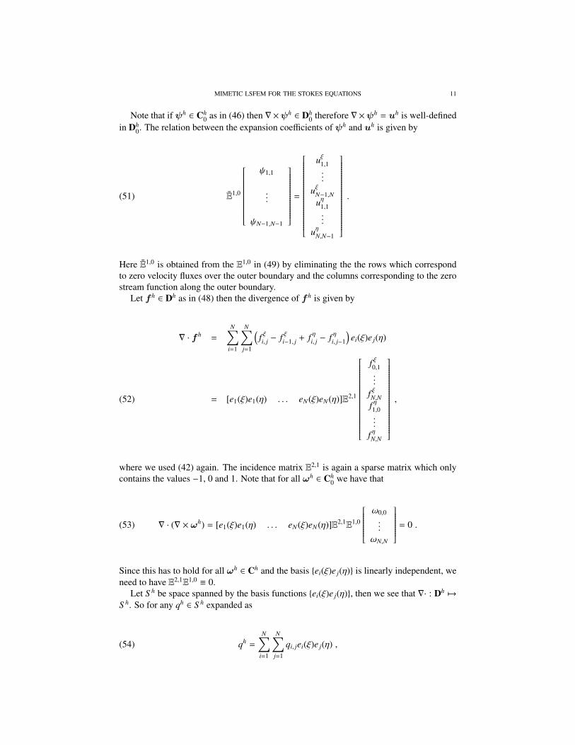
Let f h ∈ Dh, then it can be expanded as
f h =
∑Ni=0
∑Nj=1 f ξi, jhi(ξ)e j(η)∑N
i=1∑N
j=0 f ηi, jei(ξ)h j(η)
=
[h0(ξ)e1(η) . . . hN(ξ)eN(η) 0 . . . 0
0 . . . 0 e1(ξ)h0(η) . . . eN(ξ)hN(η)
]
f ξ0,1...
f ξN,Nf η1,0...
f ηN,N
.(48)
Since both ∇ × ωh ∈ Dh and f h ∈ Dh, the equality ∇ × ωh = f h makes sense in Dh. If weequate (47) and (48), we obtain
(49) E1,0
ω0,0
...
ωN,N
=
f ξ0,1...
f ξN,Nf η1,0...
f ηN,N
,
independently of the basis functions! So ∇× can be discretized by the sparse incidencematrix E1,0 which only contains the entries −1, 0 and 1. This incidence matrix is indepen-dent of the mesh width, the shape of the mesh – you can stretch, twist, shear the grid butthe incidence matrix remains the same – and it is independent of the order of the scheme.E1,0 represents the purely topological part of the derivative. All metric properties, size andshape of the grid and the order of the scheme, are contained in the basis functions.
The space Dh0 is obtained from Dh by setting all fluxes over the outer boundary to zero.
An element uh ∈ Dh0 is therefore represented as
uh =
∑N−1i=1
∑Nj=1 uξi, jhi(ξ)e j(η)∑N
i=1∑N−1
j=1 uηi, jei(ξ)h j(η)
=
[h1(ξ)e1(η) . . . hN−1(ξ)eN(η) 0 . . . 0
0 . . . 0 e1(ξ)h1(η) . . . eN(ξ)hN−1(η)
]
uξ1,1...
uξN−1,Nuη1,1...
uηN,N−1
.(50)
MIMETIC LSFEM FOR THE STOKES EQUATIONS 11
Note that if ψh ∈ Ch0 as in (46) then ∇×ψh ∈ Dh
0 therefore ∇×ψh = uh is well-definedin Dh
0. The relation between the expansion coefficients of ψh and uh is given by
(51) E1,0
ψ1,1
...
ψN−1,N−1
=
uξ1,1...
uξN−1,Nuη1,1...
uηN,N−1
.
Here E1,0 is obtained from the E1,0 in (49) by eliminating the the rows which correspondto zero velocity fluxes over the outer boundary and the columns corresponding to the zerostream function along the outer boundary.
Let f h ∈ Dh as in (48) then the divergence of f h is given by
∇ · f h =
N∑i=1
N∑j=1
(f ξi, j − f ξi−1, j + f ηi, j − f ηi, j−1
)ei(ξ)e j(η)
= [e1(ξ)e1(η) . . . eN(ξ)eN(η)]E2,1
f ξ0,1...
f ξN,Nf η1,0...
f ηN,N
,(52)
where we used (42) again. The incidence matrix E2,1 is again a sparse matrix which onlycontains the values −1, 0 and 1. Note that for all ωh ∈ Ch
0 we have that
(53) ∇ · (∇ × ωh) = [e1(ξ)e1(η) . . . eN(ξ)eN(η)]E2,1E1,0
ω0,0...
ωN,N
= 0 .
Since this has to hold for all ωh ∈ Ch and the basis ei(ξ)e j(η) is linearly independent, weneed to have E2,1E1,0 ≡ 0.
Let S h be space spanned by the basis functions ei(ξ)e j(η), then we see that ∇· : Dh 7→
S h. So for any qh ∈ S h expanded as
(54) qh =
N∑i=1
N∑j=1
qi, jei(ξ)e j(η) ,
12 MARC GERRITSMA AND PAVEL BOCHEV
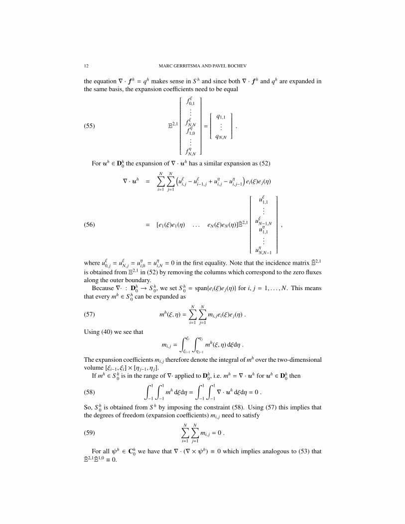
the equation ∇ · f h = qh makes sense in S h and since both ∇ · f h and qh are expanded inthe same basis, the expansion coefficients need to be equal
(55) E2,1
f ξ0,1...
f ξN,Nf η1,0...
f ηN,N
=
q1,1...
qN,N
.
For uh ∈ Dh0 the expansion of ∇ · uh has a similar expansion as (52)
∇ · uh =
N∑i=1
N∑j=1
(uξi, j − uξi−1, j + uηi, j − uηi, j−1
)ei(ξ)e j(η)
= [e1(ξ)e1(η) . . . eN(ξ)eN(η)]E2,1
uξ1,1...
uξN−1,Nuη1,1...
uηN,N−1
,(56)
where uξ0, j = uξN, j = uηi,0 = uηi,N = 0 in the first equality. Note that the incidence matrix E2,1
is obtained from E2,1 in (52) by removing the columns which correspond to the zero fluxesalong the outer boundary.
Because ∇· : Dh0 → S h
0, we set S h0 = spanei(ξ)e j(η) for i, j = 1, . . . ,N. This means
that every mh ∈ S h0 can be expanded as
(57) mh(ξ, η) =
N∑i=1
N∑j=1
mi, jei(ξ)e j(η) .
Using (40) we see that
mi, j =
∫ ξi
ξi−1
∫ η j
η j−1
mh(ξ, η) dξdη .
The expansion coefficients mi, j therefore denote the integral of mh over the two-dimensionalvolume [ξi−1, ξi] × [η j−1, η j].
If mh ∈ S h0 is in the range of ∇· applied to Dh
0, i.e. mh = ∇ · uh for uh ∈ Dh0 then
(58)∫ 1
−1
∫ 1
−1mh dξdη =
∫ 1
−1
∫ 1
−1∇ · uh dξdη = 0 .
So, S h0 is obtained from S h by imposing the constraint (58). Using (57) this implies that
the degrees of freedom (expansion coefficients) mi, j need to satisfy
(59)N∑
i=1
N∑j=1
mi, j = 0 .
For all ψh ∈ Ch0 we have that ∇ · (∇ × ψh) ≡ 0 which implies analogous to (53) that
E2,1E1,0 ≡ 0.
MIMETIC LSFEM FOR THE STOKES EQUATIONS 13
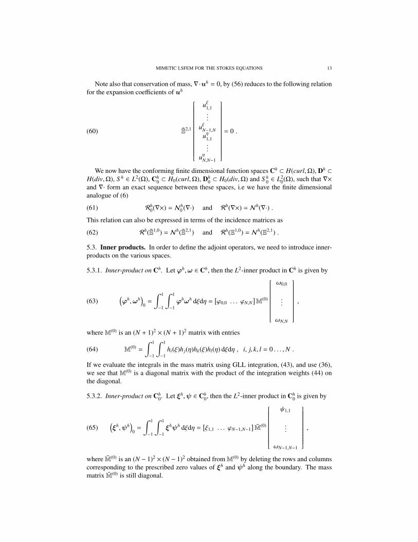
Note also that conservation of mass, ∇·uh = 0, by (56) reduces to the following relationfor the expansion coefficients of uh
(60) E2,1
uξ1,1...
uξN−1,Nuη1,1...
uηN,N−1
= 0 .
We now have the conforming finite dimensional function spaces Ch ⊂ H(curl,Ω), Dh ⊂
H(div,Ω), S h ∈ L2(Ω), Ch0 ⊂ H0(curl,Ω), Dh
0 ⊂ H0(div,Ω) and S h0 ∈ L2
0(Ω), such that ∇×and ∇· form an exact sequence between these spaces, i.e we have the finite dimensionalanalogue of (6)
(61) Rh0(∇×) = Nh
0 (∇·) and Rh(∇×) = Nh(∇·) .
This relation can also be expressed in terms of the incidence matrices as
(62) Rh(E1,0) = Nh(E2,1) and Rh(E1,0) = Nh(E2,1) .
5.3. Inner products. In order to define the adjoint operators, we need to introduce inner-products on the various spaces.
5.3.1. Inner-product on Ch. Let ϕh,ω ∈ Ch, then the L2-inner product in Ch is given by
(63)(ϕh,ωh
)0
=
∫ 1
−1
∫ 1
−1ϕhωh dξdη =
[ϕ0,0 . . . ϕN,N
]M(0)
ω0,0
...
ωN,N
,
whereM(0) is an (N + 1)2 × (N + 1)2 matrix with entries
(64) M(0) =
∫ 1
−1
∫ 1
−1hi(ξ)h j(η)hk(ξ)hl(η) dξdη , i, j, k, l = 0 . . . ,N .
If we evaluate the integrals in the mass matrix using GLL integration, (43), and use (36),we see that M(0) is a diagonal matrix with the product of the integration weights (44) onthe diagonal.
5.3.2. Inner-product on Ch0. Let ξh,ψ ∈ Ch
0, then the L2-inner product in Ch0 is given by
(65)(ξh,ψh
)0
=
∫ 1
−1
∫ 1
−1ξhψh dξdη =
[ξ1,1 . . . ϕN−1,N−1
]M(0)
ψ1,1
...
ωN−1,N−1
,
where M(0) is an (N − 1)2 × (N − 1)2 obtained fromM(0) by deleting the rows and columnscorresponding to the prescribed zero values of ξh and ψh along the boundary. The massmatrix M(0) is still diagonal.
14 MARC GERRITSMA AND PAVEL BOCHEV
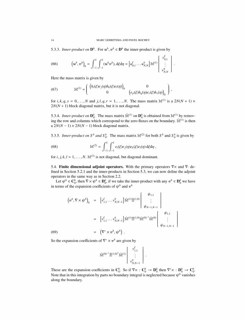
5.3.3. Inner-product on Dh. For uh,vh ∈ Dh the inner-product is given by
(66)(uh,vh
)0
=
∫ 1
−1
∫ 1
−1(uhvh), dξdη =
[uξ0,1 . . . u
ηN,N
]M(1)
vξ0,1...
vηN,N
.Here the mass matrix is given by
(67) M(1) =
(hi(ξ)e j(η)hk(ξ)el(η)
)0
00
(ep(ξ)hq(η)er(ξ)hs(η)
)0
,for i, k, q, s = 0, . . . ,N and j, l, q, r = 1, . . . ,N. The mass matrix M(1) is a 2N(N + 1) ×2N(N + 1) block diagonal matrix, but it is not diagonal.
5.3.4. Inner-product on Dh0. The mass matrix M(1) on Dh
0 is obtained fromM(1) by remov-ing the row and columns which correspond to the zero fluxes on the boundary. M(1) is thena 2N(N − 1) × 2N(N − 1) block diagonal matrix.
5.3.5. Inner-product on S h and S h0. The mass matrixM(2) for both S h and S h
0 is given by
(68) M(2) =
∫ 1
−1
∫ 1
−1ei(ξ)e j(η)ek(ξ)el(η) dξdη ,
for i, j, k, l = 1, . . . ,N. M(2) is not diagonal, but diagonal dominant.
5.4. Finite dimensional adjoint operators. With the primary operators ∇× and ∇· de-fined in Section 5.2.1 and the inner-products in Section 5.3, we can now define the adjointoperators in the same way as in Section 2.2.
Let ψh ∈ Ch0, then ∇ ×ψh ∈ Dh
0, if we take the inner-product with any vh ∈ Dh0 we have
in terms of the expansion coefficients of ψh and vh
(vh,∇ ×ψh
)0
=[vξ1,1 . . . v
ηN,N−1
]M(1)E(1,0)
ψ1,1...
ψN−1,N−1
=
[vξ1,1 . . . v
ηN,N−1
]M(1)E(1,0)M(0)−1
M(0)
ψ1,1...
ψN−1,N−1
=
(∇∗ × vh,ψh
).(69)
So the expansion coefficients of ∇∗ × vh are given by
M(0)−1E(1,0)T
M(1)
vξ1,1...
vηN,N−1
.These are the expansion coefficients in Ch
0. So if ∇× : Ch0 → Dh
0 then ∇∗× : Dh0 → Ch
0.Note that in this integration by parts no boundary integral is neglected becauseψh vanishesalong the boundary.

MIMETIC LSFEM FOR THE STOKES EQUATIONS 15
Let uh ∈ Dh0 then ∇ · uh ∈ S h
0. If we take the inner-product with any φ ∈ S h0, we obtain
in terms of the expansion coefficients of uh and φh
(φh,∇ · uh
)0
=[φ1,1 . . . φN,N
]M(2)E2,1
uξ1,1...
uηN,N−1
=
[φ1,1 . . . φN,N
]M(2)E2,1M(1)−1
M(1)
uξ1,1...
uηN,N−1
=
(∇∗φ,uh
)0.(70)
Therefore, the expansion coefficients of ∇∗φ ∈ Dh0 are given by
M(1)−1E2,1TM(2)
φ1,1...
φN,N
.These are expansion coefficients in Dh
0 so we use the basis functions in Dh0 to expand ∇∗φh,
such that ∇∗ : S h0 → Dh
0. Note that again no boundary integrals were neglected, becauseuh · n = 0 for all uh ∈ Dh
0.From
0 =(∇ · (∇ × ψh), φh
)0
=(∇ × ψh,∇∗φh
)0
=(ψh,∇∗ × (∇∗φh)
)0,
it follows thatRh
0(∇∗) = Nh0 (∇∗×) and Rh
0(∇×) ⊥ Rh0(∇∗) .
This can also be seen from the expansion coefficients. The expansion coefficients ~φ of φh
are mapped on the expansion coefficients M(1)−1E2,1TM(2)~φ of ∇∗φh, which are then mapped
by to the expansion coefficients M(0)−1E(1,0)T
M(1)M(1)−1E2,1TM(2)~φ of∇∗×∇∗φh which is zero
because E(1,0)TE2,1T
=(E(1,0)E2,1
)≡ 0.
We can now write the orthogonal decomposition of any uh ∈ Dh0 in terms of the expan-
sion coefficients. Let ψh ∈ Ch0 and φh ∈ S h
0 such that
uh = ∇ × ψh + ∇∗φh .
Then we have for the expansion coefficients
~u = E1,0~ψ + M(1)−1E(2,1)T
M(2)~φ ,
from which we can obtain the expansion coefficients ~ψ and ~φ by solving the symmetricsystems
M(2)E2,1~u = M(2)E2,1M(1)−1E(2,1)T
M(2)~φ and E1,0TM(1)~u = E1,0T
M(1)E1,0~ψ .
Ch0 Dh
0 S h0
∇×
∇∗×
∇·
∇∗
Or in terms of the expansion coefficients in these space
E(Ch0) E(Dh
0) E(S h0)
E1,0
M(0)−1E1,0T
M(1)
E2,1
M(1)−1E2,1T
M(2)
16 MARC GERRITSMA AND PAVEL BOCHEV
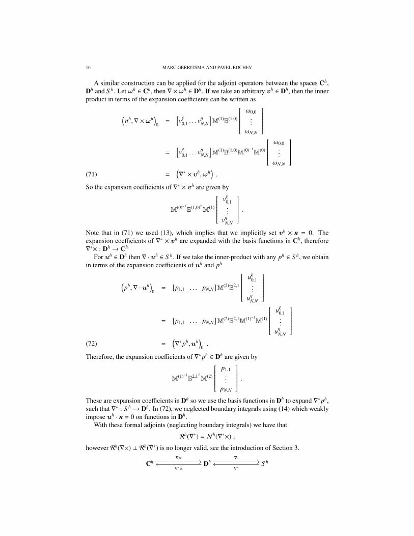
A similar construction can be applied for the adjoint operators between the spaces Ch,Dh and S h. Let ωh ∈ Ch, then ∇ ×ωh ∈ Dh. If we take an arbitrary vh ∈ Dh, then the innerproduct in terms of the expansion coefficients can be written as
(vh,∇ × ωh
)0
=[vξ0,1 . . . v
ηN,N
]M(1)E(1,0)
ω0,0...
ωN,N
=
[vξ0,1 . . . v
ηN,N
]M(1)E(1,0)M(0)−1
M(0)
ω0,0...
ωN,N
=
(∇∗ × vh,ωh
).(71)
So the expansion coefficients of ∇∗ × vh are given by
M(0)−1E(1,0)T
M(1)
vξ0,1...
vηN,N
.Note that in (71) we used (13), which implies that we implicitly set vh × n = 0. Theexpansion coefficients of ∇∗ × vh are expanded with the basis functions in Ch, therefore∇∗× : Dh → Ch
For uh ∈ Dh then ∇ ·uh ∈ S h. If we take the inner-product with any ph ∈ S h, we obtainin terms of the expansion coefficients of uh and ph
(ph,∇ · uh
)0
=[p1,1 . . . pN,N
]M(2)E2,1
uξ0,1...
uηN,N
=
[p1,1 . . . pN,N
]M(2)E2,1M(1)−1
M(1)
uξ0,1...
uηN,N
=
(∇∗ph,uh
)0.(72)
Therefore, the expansion coefficients of ∇∗ph ∈ Dh are given by
M(1)−1E2,1TM(2)
p1,1...
pN,N
.These are expansion coefficients in Dh so we use the basis functions in Dh to expand ∇∗ph,such that ∇∗ : S h → Dh. In (72), we neglected boundary integrals using (14) which weaklyimpose uh · n = 0 on functions in Dh.
With these formal adjoints (neglecting boundary integrals) we have that
Rh(∇∗) = Nh(∇∗×) ,
however Rh(∇×) ⊥ Rh(∇∗) is no longer valid, see the introduction of Section 3.
Ch Dh S h∇×
∇∗×
∇·
∇∗
MIMETIC LSFEM FOR THE STOKES EQUATIONS 17
Or in terms of the expansion coefficients in these space
E(Ch) E(Dh) E(S h)E1,0
M(0)−1E1,0T
M(1)
E2,1
M(1)−1E2,1T
M(2)
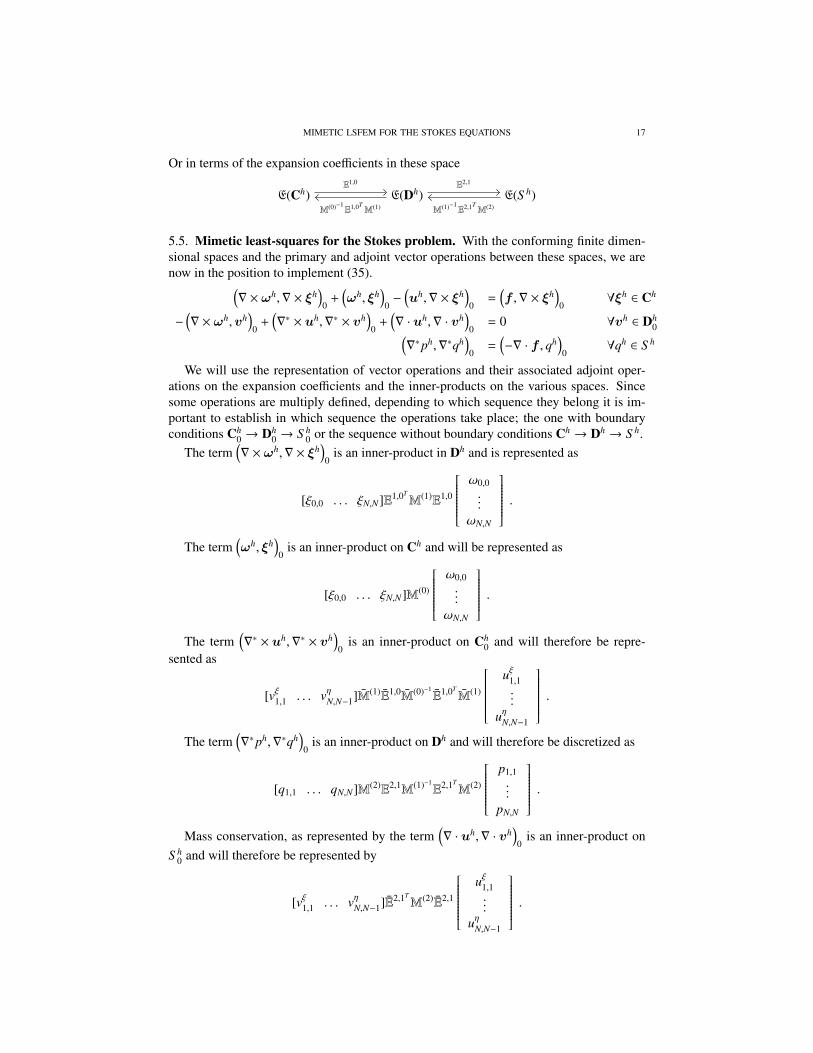
5.5. Mimetic least-squares for the Stokes problem. With the conforming finite dimen-sional spaces and the primary and adjoint vector operations between these spaces, we arenow in the position to implement (35).(
∇ × ωh,∇ × ξh)
0+
(ωh, ξh
)0−
(uh,∇ × ξh
)0
=(f ,∇ × ξh
)0
∀ξh ∈ Ch
−(∇ × ωh,vh
)0
+(∇∗ × uh,∇∗ × vh
)0
+(∇ · uh,∇ · vh
)0
= 0 ∀vh ∈ Dh0(
∇∗ph,∇∗qh)
0=
(−∇ · f , qh
)0
∀qh ∈ S h
We will use the representation of vector operations and their associated adjoint oper-ations on the expansion coefficients and the inner-products on the various spaces. Sincesome operations are multiply defined, depending to which sequence they belong it is im-portant to establish in which sequence the operations take place; the one with boundaryconditions Ch
0 → Dh0 → S h
0 or the sequence without boundary conditions Ch → Dh → S h.The term
(∇ × ωh,∇ × ξh
)0
is an inner-product in Dh and is represented as
[ξ0,0 . . . ξN,N]E1,0TM(1)E1,0
ω0,0...
ωN,N
.The term
(ωh, ξh
)0
is an inner-product on Ch and will be represented as
[ξ0,0 . . . ξN,N]M(0)
ω0,0...
ωN,N
.The term
(∇∗ × uh,∇∗ × vh
)0
is an inner-product on Ch0 and will therefore be repre-
sented as
[vξ1,1 . . . vηN,N−1]M(1)E1,0M(0)−1E1,0TM(1)
uξ1,1...
uηN,N−1
.The term
(∇∗ph,∇∗qh
)0
is an inner-product on Dh and will therefore be discretized as
[q1,1 . . . qN,N]M(2)E2,1M(1)−1E2,1TM(2)
p1,1...
pN,N
.Mass conservation, as represented by the term
(∇ · uh,∇ · vh
)0
is an inner-product onS h
0 and will therefore be represented by
[vξ1,1 . . . vηN,N−1]E2,1TM(2)E2,1
uξ1,1...
uηN,N−1
.
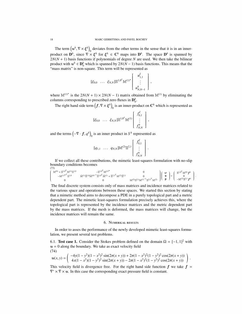
18 MARC GERRITSMA AND PAVEL BOCHEV
The term(uh,∇ × ξh
)0
deviates from the other terms in the sense that it is in an inner-product on Dh, since ∇ × ξh for ξh ∈ Ch maps into Dh. The space Dh is spanned by2N(N + 1) basis functions if polynomials of degree N are used. We then take the bilinearproduct with uh ∈ Dh
0 which is spanned by 2N(N − 1) basis functions. This means that the“mass matrix” is non-square. This term will be represented as
[ξ0,0 . . . ξN,N]E1,0TM(1)?
uξ1,1...
uηN,N−1
,where M(1)? is the 2N(N + 1) × 2N(N − 1) matrix obtained from M(1) by eliminating thecolumns corresponding to prescribed zero fluxes in Dh
0.The right hand side term
(f ,∇ × ξh
)0
is an inner-product on Ch which is represented as
[ξ0,0 . . . ξN,N]E1,0TM(1)
f ξ0,1...
f ηN,N
,and the terms
(−∇ · f , qh
)0
is an inner product in S h represented as
[q1,1 . . . qN,N]M(2)E2,1
f ξ0,1...
f ηN,N
.If we collect all these contributions, the mimetic least-squares formulation with no-slip
boundary conditions becomes(73)M(0) + E1,0T
M(1)E1,0 −E1,0TM(1)? 0
−M(1)?TE1,0 M(1)E1,0M(0)−1
E1,0TM(1) + E2,1T
M(2)E2,1 00 0 M(2)E2,1M(1)−1
E2,1TM(2)
ωup
=
E1,0TM(0)f h
0−M(2)E2,1f h
.The final discrete system consists only of mass matrices and incidence matrices related tothe various space and operations between these spaces. We started this section by statingthat a mimetic method aims to decompose a PDE in a purely topological part and a metricdependent part. The mimetic least-squares formulation precisely achieves this, where thetopological part is represented by the incidence matrices and the metric dependent partby the mass matrices. If the mesh is deformed, the mass matrices will change, but theincidence matrices will remain the same.
6. Numerical results
In order to asses the performance of the newly developed mimetic least-squares formu-lation, we present several test problems.
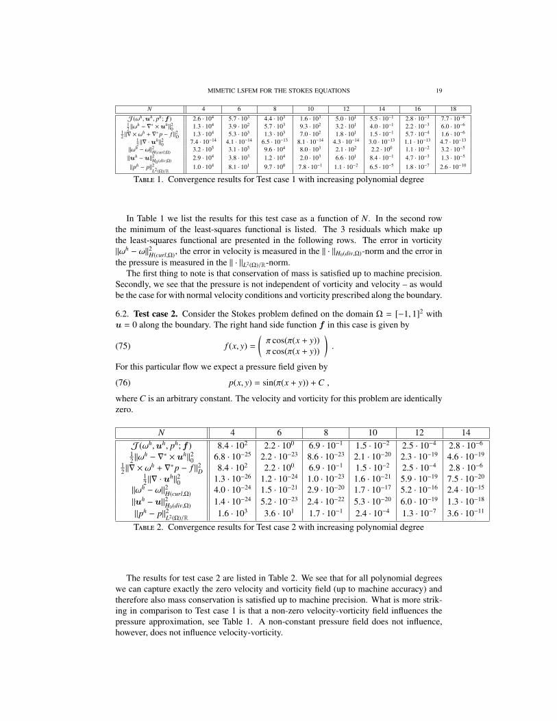
6.1. Test case 1. Consider the Stokes problem defined on the domain Ω = [−1, 1]2 withu = 0 along the boundary. We take as exact velocity field(74)
u(x, y) =
(−4y(1 − y2)(1 − x2)2 sin(2π(x + y)) + 2π(1 − x2)2(1 − y2)2 cos(2π(x + y))4x(1 − x2)(1 − y2)2 sin(2π(x + y)) − 2π(1 − x2)2(1 − y2)2 cos(2π(x + y))
).
This velocity field is divergence free. For the right hand side function f we take f =
∇∗ × ∇ × u. In this case the corresponding exact pressure field is constant.
MIMETIC LSFEM FOR THE STOKES EQUATIONS 19
N 4 6 8 10 12 14 16 18
J(ωh,uh, ph;f ) 2.6 · 104 5.7 · 103 4.4 · 103 1.6 · 103 5.0 · 101 5.5 · 10−1 2.8 · 10−3 7.7 · 10−6
12 ‖ω
h − ∇∗ ×uh‖20 1.3 · 104 3.9 · 102 5.7 · 103 9.3 · 102 3.2 · 101 4.0 · 10−1 2.2 · 10−3 6.0 · 10−6
12 ‖∇ × ω
h + ∇∗p − f ‖2D 1.3 · 104 5.3 · 103 1.3 · 103 7.0 · 102 1.8 · 101 1.5 · 10−1 5.7 · 10−4 1.6 · 10−6
12 ‖∇ ·u
h‖20 7.4 · 10−14 4.1 · 10−14 6.5 · 10−13 8.1 · 10−14 4.3 · 10−14 3.0 · 10−13 1.1 · 10−13 4.7 · 10−13
‖ωh − ω‖2H(curl,Ω) 3.2 · 105 3.1 · 105 9.6 · 104 8.0 · 103 2.1 · 102 2.2 · 100 1.1 · 10−2 3.2 · 10−5
‖uh −u‖2H0(div,Ω) 2.9 · 104 3.8 · 103 1.2 · 104 2.0 · 103 6.6 · 101 8.4 · 10−1 4.7 · 10−3 1.3 · 10−5
‖ph − p‖2L2(Ω)/R
1.0 · 104 8.1 · 101 9.7 · 100 7.8 · 10−1 1.1 · 10−2 6.5 · 10−5 1.8 · 10−7 2.6 · 10−10
Table 1. Convergence results for Test case 1 with increasing polynomial degree
In Table 1 we list the results for this test case as a function of N. In the second rowthe minimum of the least-squares functional is listed. The 3 residuals which make upthe least-squares functional are presented in the following rows. The error in vorticity‖ωh − ω‖2H(curl,Ω), the error in velocity is measured in the ‖ · ‖H0(div,Ω)-norm and the error inthe pressure is measured in the ‖ · ‖L2(Ω)/R-norm.
The first thing to note is that conservation of mass is satisfied up to machine precision.Secondly, we see that the pressure is not independent of vorticity and velocity – as wouldbe the case for with normal velocity conditions and vorticity prescribed along the boundary.
6.2. Test case 2. Consider the Stokes problem defined on the domain Ω = [−1, 1]2 withu = 0 along the boundary. The right hand side function f in this case is given by
(75) f (x, y) =
(π cos(π(x + y))π cos(π(x + y))
).
For this particular flow we expect a pressure field given by
(76) p(x, y) = sin(π(x + y)) + C ,
where C is an arbitrary constant. The velocity and vorticity for this problem are identicallyzero.
N 4 6 8 10 12 14J(ωh,uh, ph;f ) 8.4 · 102 2.2 · 100 6.9 · 10−1 1.5 · 10−2 2.5 · 10−4 2.8 · 10−6
12‖ω
h − ∇∗ × uh‖20 6.8 · 10−25 2.2 · 10−23 8.6 · 10−23 2.1 · 10−20 2.3 · 10−19 4.6 · 10−19
12 ‖∇ × ω
h + ∇∗p − f ‖2D 8.4 · 102 2.2 · 100 6.9 · 10−1 1.5 · 10−2 2.5 · 10−4 2.8 · 10−6
12‖∇ · u
h‖20 1.3 · 10−26 1.2 · 10−24 1.0 · 10−23 1.6 · 10−21 5.9 · 10−19 7.5 · 10−20
‖ωh − ω‖2H(curl,Ω) 4.0 · 10−24 1.5 · 10−21 2.9 · 10−20 1.7 · 10−17 5.2 · 10−16 2.4 · 10−15
‖uh − u‖2H0(div,Ω) 1.4 · 10−24 5.2 · 10−23 2.4 · 10−22 5.3 · 10−20 6.0 · 10−19 1.3 · 10−18
‖ph − p‖2L2(Ω)/R 1.6 · 103 3.6 · 101 1.7 · 10−1 2.4 · 10−4 1.3 · 10−7 3.6 · 10−11
Table 2. Convergence results for Test case 2 with increasing polynomial degree
The results for test case 2 are listed in Table 2. We see that for all polynomial degreeswe can capture exactly the zero velocity and vorticity field (up to machine accuracy) andtherefore also mass conservation is satisfied up to machine precision. What is more strik-ing in comparison to Test case 1 is that a non-zero velocity-vorticity field influences thepressure approximation, see Table 1. A non-constant pressure field does not influence,however, does not influence velocity-vorticity.
20 MARC GERRITSMA AND PAVEL BOCHEV
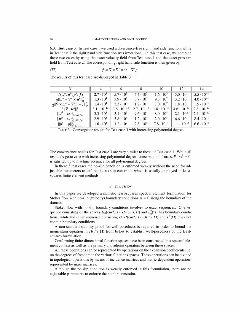
6.3. Test case 3. In Test case 1 we used a divergence-free right hand side function, whilein Test case 2 the right hand side function was irrotational. In this test case, we combinethese two cases by using the exact velocity field from Test case 1 and the exact pressurefield from Test case 2. The corresponding right hand side function is then given by
(77) f = ∇ × ∇∗ × u + ∇∗p .
The results of this test case are displayed in Table 3
N 4 6 8 10 12 14J(ωh,uh, ph;f ) 2.7 · 104 5.7 · 103 4.4 · 103 1.6 · 103 5.0 · 101 5.5 · 10−1
12‖ω
h − ∇∗ × uh‖20 1.3 · 104 3.9 · 102 5.7 · 103 9.3 · 102 3.2 · 101 4.0 · 10−1
12 ‖∇ × ω
h + ∇∗p − f ‖2D 1.4 · 104 5.3 · 103 1.2 · 103 7.0 · 102 1.8 · 101 1.5 · 10−1
12‖∇ · u
h‖20 3.1 · 10−13 3.6 · 10−14 2.7 · 10−13 1.8 · 10−13 4.6 · 10−13 2.8 · 10−13
‖ωh − ω‖2H(curl,Ω) 3.3 · 105 3.1 · 105 9.6 · 104 8.0 · 103 2.1 · 102 2.4 · 10−15
‖uh − u‖2H0(div,Ω) 2.9 · 104 3.8 · 103 1.2 · 104 2.0 · 103 6.6 · 101 8.4 · 10−1
‖ph − p‖2L2(Ω)/R 1.6 · 104 1.2 · 102 9.8 · 100 7.8 · 10−1 1.1 · 10−2 6.6 · 10−5
Table 3. Convergence results for Test case 3 with increasing polynomial degree
The convergence results for Test case 3 are very similar to those of Test case 1. While allresiduals go to zero with increasing polynomial degree, conservation of mass, ∇ · uh = 0,is satisfied up to machine accuracy for all polynomial degrees
In these 3 test cases the no-slip condition is enforced weakly without the need for ad-justable parameters to enforce he no-slip constraint which is usually employed in least-squares finite element methods.
7. Discussion
In this paper we developed a mimetic least-squares spectral element formulation forStokes flow with no-slip (velocity) boundary conditions u = 0 along the boundary of thedomain.
Stokes flow with no-slip boundary conditions involves to exact sequences. One se-quence consisting of the spaces H0(curl,Ω), H0(curl,Ω) and L2
0(Ω) has boundary condi-tions, while the other sequence consisting of H(curl,Ω), H(div,Ω) and L2(Ω) does notcontain boundary conditions.
A non-standard stability proof for well-posedness is required in order to bound themomentum equation in H(div,Ω) from below to establish well-posedness of the least-squares formulation.
Conforming finite dimensional function spaces have been constructed in a spectral ele-ment context as well as the primary and adjoint operators between these spaces.
All these operations can be represented by operations on the expansion coefficients, i.e.on the degrees of freedom in the various functions spaces. These operations can be dividedin topological operations by means of incidence matrices and metric-dependent operationsrepresented by mass matrices.
Although the no-slip condition is weakly enforced in this formulation, there are noadjustable parameters to enforce the no-slip constraint.
MIMETIC LSFEM FOR THE STOKES EQUATIONS 21
Numerical tests for non-trivial right-hand side functions reveal that the method is con-vergent and that mass is conserved for all polynomial degrees. Approximation only takesplace in the momentum equation and the definition of vorticity.
Future work will focus on multi-element methods, curvilinear grids and error estimatesbased on the current least-squares formalism.
Acknowledgments
This material is based upon work supported by the U.S. Department of Energy, Officeof Science, Office of Advanced Scientific Computing Research.
References
[1] P. Bochev and M. Gerritsma. A spectral mimetic least-squares method. Computersand Mathematics with Applications, 86:1480–1502, 2014.
[2] P. Bochev and M. Gunzburger. Analysis of least-squares finite element methods forthe Stokes equations. Math. Comp., 63:479–506, 1994.
[3] P. Bochev and M. Gunzburger. A locally conservative mimetic least-squares finiteelement method for the Stokes equations. In I. Lirkov, S. Margenov, and J. Was-niewski, editors, In proceedings LSSC 2009, volume 5910 of Springer Lecture Notesin Computer Science, pages 637–644, 2009.
[4] P. Bochev and M. Gunzburger. Least-Squares finite element methods, volume 166 ofApplied Mathematical Sciences. Springer Verlag, 2009.
[5] P. Bochev and J. Hyman. Principles of mimetic disrcertizations of differential oper-ators. In R. N. D. Arnold, P. Bochev and M. Shashkov, editors, Compatible SpatialDiscretizations, volume 42 of The IMA volumes in Mathematics and its Applications,pages 89–119. Springer Verlag, 2006.
[6] P. Bochev, J. Lai, and L. Olson. A locally conservative, discontinuous least-squaresfinite element method for the Stokes equations. International Journal for NumericalMethods in Fluids, 68(6):782–804, 2012.
[7] P. Bochev, J. Lai, and L. Olson. A non-conforming least-squares finite elementmethod for incompressible fluid flow problems. International Journal for Numer-ical Methods in Fluids, 72(3):375–402, 2013.
[8] P. B. Bochev. Negative norm least-squares methods for the velocity-vorticity-pressureNavier–Stokes equations. Numerical Methods for Partial Differential Equations,15(2):237–256, 1999.
[9] J. Bonelle and A. Ern. Analysis of compatible discrete operator schemes for thestokes equations on polyhedral meshes. IMA Journal of Numerical Analysis, toappear:1–26, 2014.
[10] A. Bossavit. On the geometry of electromagnetism. Journal of the Japanese Societyof Applied Electromagnetics and Mechanics, 6:17–28 (no 1), 114–23 (no 2), 233–40(no 3), 318–26 (no 4), 1998.
[11] A. Bossavit. Computational electromagnetism and geometry. Journal of the JapaneseSociety of Applied Electromagnetics and Mechanics, 7, 8:150–9 (no 1), 294–301 (no2), 401–408 (no 3), 102–109 (no 4), 203–209 (no 5), 372–377 (no 6), 1999, 2000.
[12] A. Q. T. Z. C. Canuto, M.Y. Hussaini. Spectral Methods, fundamentals in singledomains. Springer-Verlag, 2006.
[13] M. Desbrun, A. Hirani, M. Leok, and J. Marsden. Discrete Exterior Calculus. Arxivpreprint math/0508341, 2005.

22 MARC GERRITSMA AND PAVEL BOCHEV
[14] M. Gerritsma. Edge functions for spectral element methods. In J. Hesthaven andE. Rønquist, editors, Spectral and High Order Methods for Partial Differential Equa-tions, volume 76 of Springer Lecture Notes in Computational Science and Engineer-ing, pages 199–208, 2011.
[15] J. Kreeft, A. Palha, and M. Gerritsma. Mimetic framework on curvilinear quadrilat-erals of arbitrary order. arXiv:1111.4304, 2011.
[16] A. Lemoine, J.-P. Caltagirone, M. Azaıez, and S. Vincent. Discrete Helmholtz-Hodgedecomposition on polyhedral meshes using compatible discrete operators. Journal ofScientific Computing, In Press, 2014.
[17] K. Lipnikov, G. Manzini, and M. Shashkov. Mimetic finite difference method. Jour-nal of Computational Physics, 254:1163–1227, 2014.
[18] M. Seslija, A. van der Schaft, and J. Scherpen. Discrete exterior geometry approach tostructure-preserving discretization of distributed port-hamiltonian systems. Journalof Geometry and Physics, 62(6):1509–1531, 2012.
[19] M. E. Taylor. Partial Differential Equations. Basic Theory. Number 23 in Texts inApplied Mathematics. Springer Berlin / Heidelberg, 1999.
[20] E. Tonti. On the formal structure of physical theories. preprint of the Italian NationalResearch Council, 1975.
[21] E. Tonti. The Common Structure of Physical Theories. Springer, to appear.
Delft University of Technology, Faculty of Aerospace Engineering,Kluyverweg 2, 2629 HT Delft, The Netherlands.E-mail address: [email protected], [email protected]
Sandia National Laboratories,3
Center for Computing Research, Mail Stop 1320, Albuquerque, NM 87185, USA
3Sandia is a multiprogram laboratory operated by Sandia Corporation, a Lockheed Martin Company, for theU.S. Department of Energy under contract DE-AC04-94-AL85000.