Lectures IIT Kanpur, India Lecture 1: @=@x and dx › math › workshop-and-conference › WMSEM ›...
71
Lectures IIT Kanpur, India Lecture 1: ∂/∂ x and dx A new meaning for familiar symbols Marc Gerritsma [email protected] Department of Aerospace Engineering Delft University of Technology 23 March 2015 Marc Gerritsma (TUD) Mimetic discretizations Lecture 1 1 / 27
Transcript of Lectures IIT Kanpur, India Lecture 1: @=@x and dx › math › workshop-and-conference › WMSEM ›...
Lectures IIT Kanpur, IndiaLecture 1: ∂/∂x and dx
A new meaning for familiar symbols
Marc [email protected]
Department of Aerospace EngineeringDelft University of Technology
23 March 2015
Marc Gerritsma (TUD) Mimetic discretizations Lecture 1 1 / 27
Overview Introduction
Outline of this lecture
This short course on mimetic spectral elements consists of 6 lectures:
Lecture 1: In this lecture we will review some basic concepts from differential geometry
Lecture 2: Generalized Stokes Theorem and geometric integration
Lecture 3: Connection between continuous and discrete quantities. The Reductionoperator and the reconstruction operator.
Lecture 4: The Hodge-? operator. Finite volume, finite element methods andleast-squares methods.
Lecture 5: Application of mimetic schemes to elliptic equations. Poisson and Stokesproblem
Lecture 6: Open research questions. Collaboration.
Marc Gerritsma (TUD) Mimetic discretizations Lecture 1 2 / 27

Overview Introduction
The Poisson problemMy favorite appetizer
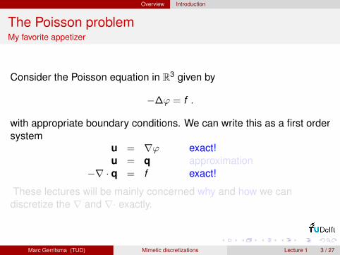
Consider the Poisson equation in R3 given by
−∆ϕ = f .
with appropriate boundary conditions. We can write this as a first ordersystem
u = ∇ϕ exact!u = q approximation
−∇ · q = f exact!
These lectures will be mainly concerned why and how we candiscretize the ∇ and ∇· exactly.
Marc Gerritsma (TUD) Mimetic discretizations Lecture 1 3 / 27

Overview Introduction
The Poisson problemMy favorite appetizer
Consider the Poisson equation in R3 given by
−∆ϕ = f .
with appropriate boundary conditions. We can write this as a first ordersystem
u = ∇ϕ exact!u = q approximation
−∇ · q = f exact!
These lectures will be mainly concerned why and how we candiscretize the ∇ and ∇· exactly.
Marc Gerritsma (TUD) Mimetic discretizations Lecture 1 3 / 27

Overview Introduction
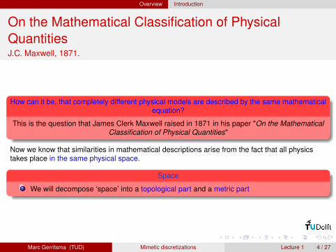
On the Mathematical Classification of PhysicalQuantitiesJ.C. Maxwell, 1871.
How can it be, that completely different physical models are described by the same mathematicalequation?
This is the question that James Clerk Maxwell raised in 1871 in his paper "On the MathematicalClassification of Physical Quantities"
Now we know that similarities in mathematical descriptions arise from the fact that all physicstakes place in the same physical space.
Space
We will decompose ‘space’ into a topological part and a metric part
Marc Gerritsma (TUD) Mimetic discretizations Lecture 1 4 / 27

Overview Introduction
On the Mathematical Classification of PhysicalQuantitiesJ.C. Maxwell, 1871.
How can it be, that completely different physical models are described by the same mathematicalequation?
This is the question that James Clerk Maxwell raised in 1871 in his paper "On the MathematicalClassification of Physical Quantities"
Now we know that similarities in mathematical descriptions arise from the fact that all physicstakes place in the same physical space.
Space
We will decompose ‘space’ into a topological part and a metric part
Marc Gerritsma (TUD) Mimetic discretizations Lecture 1 4 / 27
Space, functions & vectors
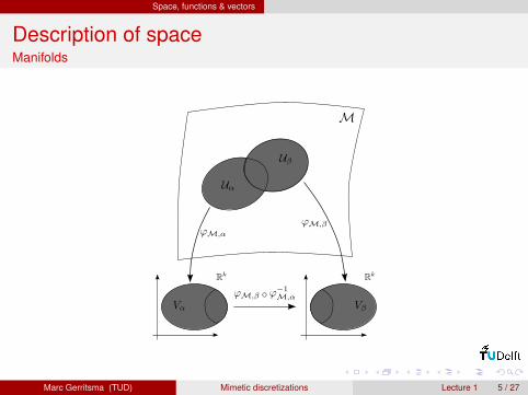
Description of spaceManifolds
Marc Gerritsma (TUD) Mimetic discretizations Lecture 1 5 / 27

Space, functions & vectors
Functions and vectors I
With the charts we can identifya point P ∈M with a k -tuple(x1, . . . , xk )
P
Marc Gerritsma (TUD) Mimetic discretizations Lecture 1 6 / 27
Space, functions & vectors
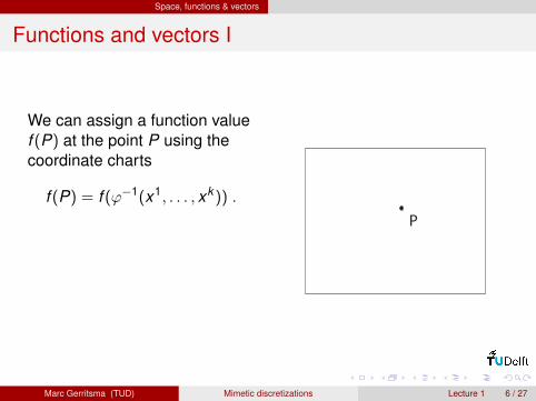
Functions and vectors I
We can assign a function valuef (P) at the point P using thecoordinate charts
f (P) = f (ϕ−1(x1, . . . , xk )) .
P
Marc Gerritsma (TUD) Mimetic discretizations Lecture 1 6 / 27

Space, functions & vectors
Functions and vectors I
A curve through the point P canparameterized by s ∈ R:
γ(s) = (γ1(s), . . . , γk (s)) ,
withγ(0) = P .
P
Marc Gerritsma (TUD) Mimetic discretizations Lecture 1 6 / 27
Space, functions & vectors
Functions and vectors I
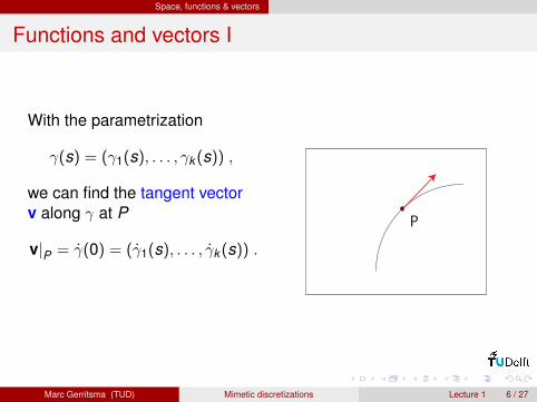
With the parametrization
γ(s) = (γ1(s), . . . , γk (s)) ,
we can find the tangent vectorv along γ at P
v|P = γ(0) = (γ1(s), . . . , γk (s)) .
P
Marc Gerritsma (TUD) Mimetic discretizations Lecture 1 6 / 27
Space, functions & vectors
Functions and vectors I
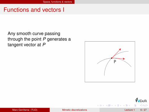
Any smooth curve passingthrough the point P generates atangent vector at P
P
Marc Gerritsma (TUD) Mimetic discretizations Lecture 1 6 / 27

Space, functions & vectors
Functions and vectors I
Every curve through P generates a tangent vector at P. Conversely,any tangent vector at the point P can be associated to a class ofcurves through the point P. The space of tangent vectors at the point Pis called the Tangent space at P, denoted by TPM
Marc Gerritsma (TUD) Mimetic discretizations Lecture 1 6 / 27

Space, functions & vectors
Functions and vectors II
If we have a k -dimensional manifold then the dimension of TPM isequal to k . A special basis for this vector space at P is obtained bytaking the coordinate curves
γ(s) = (x1, . . . , x i + s, . . . , xk ) ,
where (x1, . . . , xk ) are the local coordinates for the point P. Theassociated tangent vector is then given by
γ(s) = (0, . . . , 1︸︷︷︸i
, . . . ,0) .
This is special basis is called a coordinate basis and usually denotedby
∂
∂x i
∣∣∣∣P
:= (0, . . . , 1︸︷︷︸i
, . . . ,0)
Marc Gerritsma (TUD) Mimetic discretizations Lecture 1 7 / 27
Space, functions & vectors
Functions and vectors III
So any tangent vector can be written as a linear combination of thecoordinate basis vectors
v = v1 ∂
∂x1
∣∣∣∣P
+ . . .+ vk ∂
∂xk
∣∣∣∣P
= v i ∂
∂x i
∣∣∣∣P
It might seem strange these basis functions, but partial derivativesbehave in the same way under transformations as basis functions.
Marc Gerritsma (TUD) Mimetic discretizations Lecture 1 8 / 27
Space, functions & vectors
Functions and vectorsIntermezzo
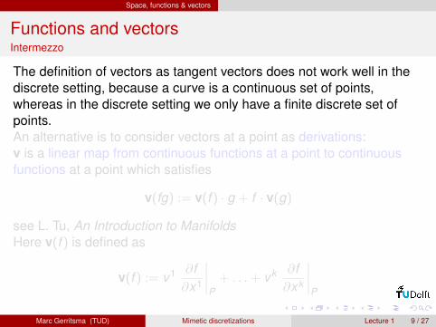
The definition of vectors as tangent vectors does not work well in thediscrete setting, because a curve is a continuous set of points,whereas in the discrete setting we only have a finite discrete set ofpoints.An alternative is to consider vectors at a point as derivations:v is a linear map from continuous functions at a point to continuousfunctions at a point which satisfies
v(fg) := v(f ) · g + f · v(g)
see L. Tu, An Introduction to ManifoldsHere v(f ) is defined as
v(f ) := v1 ∂f∂x1
∣∣∣∣P
+ . . .+ vk ∂f∂xk
∣∣∣∣P
Marc Gerritsma (TUD) Mimetic discretizations Lecture 1 9 / 27

Space, functions & vectors
Functions and vectorsIntermezzo
The definition of vectors as tangent vectors does not work well in thediscrete setting, because a curve is a continuous set of points,whereas in the discrete setting we only have a finite discrete set ofpoints.An alternative is to consider vectors at a point as derivations:v is a linear map from continuous functions at a point to continuousfunctions at a point which satisfies
v(fg) := v(f ) · g + f · v(g)
see L. Tu, An Introduction to ManifoldsHere v(f ) is defined as
v(f ) := v1 ∂f∂x1
∣∣∣∣P
+ . . .+ vk ∂f∂xk
∣∣∣∣P
Marc Gerritsma (TUD) Mimetic discretizations Lecture 1 9 / 27

Covectors
The covector I
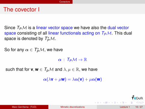
Since TPM is a linear vector space we have also the dual vectorspace consisting of all linear functionals acting on TPM. This dualspace is denoted by T ∗PM.
So for any α ∈ T ∗PM, we have
α : TPM→ R
such that for v,w ∈ TpM and λ, µ ∈ R, we have
α(λv + µw) = λα(v) + µα(w)
Marc Gerritsma (TUD) Mimetic discretizations Lecture 1 10 / 27
Covectors
The covector I
Since TPM is a linear vector space we have also the dual vectorspace consisting of all linear functionals acting on TPM. This dualspace is denoted by T ∗PM.
So for any α ∈ T ∗PM, we have
α : TPM→ R
such that for v,w ∈ TpM and λ, µ ∈ R, we have
α(λv + µw) = λα(v) + µα(w)
Marc Gerritsma (TUD) Mimetic discretizations Lecture 1 10 / 27
Covectors
The covector II
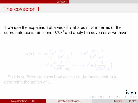
If we use the expansion of a vector v at a point P in terms of thecoordinate basis functions ∂/∂x i and apply the covector α we have
α(v) = α
(v1 ∂
∂x1
∣∣∣∣P
+ . . .+ vk ∂
∂xk
∣∣∣∣P
)= v1α
(∂
∂x1
∣∣∣∣P
)+ · · ·+ vkα
(∂
∂xk
∣∣∣∣P
)So it is sufficient to know how α acts on the basis vectors to
determine the action of α.
Marc Gerritsma (TUD) Mimetic discretizations Lecture 1 11 / 27

Covectors
The covector II
If we use the expansion of a vector v at a point P in terms of thecoordinate basis functions ∂/∂x i and apply the covector α we have
α(v) = α
(v1 ∂
∂x1
∣∣∣∣P
+ . . .+ vk ∂
∂xk
∣∣∣∣P
)= v1α
(∂
∂x1
∣∣∣∣P
)+ · · ·+ vkα
(∂
∂xk
∣∣∣∣P
)So it is sufficient to know how α acts on the basis vectors to
determine the action of α.
Marc Gerritsma (TUD) Mimetic discretizations Lecture 1 11 / 27
Covectors
The covector III
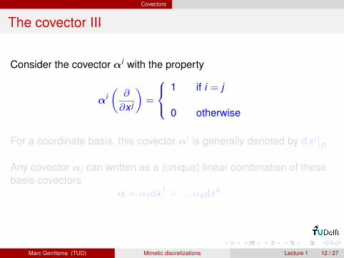
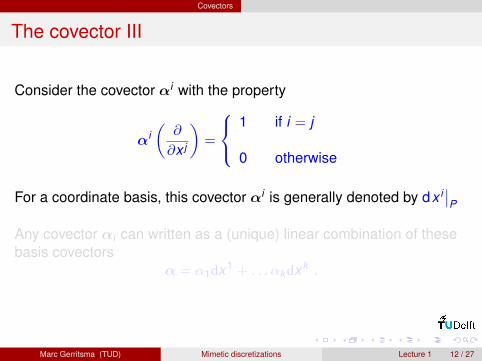
Consider the covector αi with the property
αi(∂
∂x j
)=
1 if i = j
0 otherwise
For a coordinate basis, this covector αi is generally denoted by dx i∣∣P
Any covector αi can written as a (unique) linear combination of thesebasis covectors
α = α1dx1 + . . . αk dxk .
Marc Gerritsma (TUD) Mimetic discretizations Lecture 1 12 / 27
Covectors
The covector III
Consider the covector αi with the property
αi(∂
∂x j
)=
1 if i = j
0 otherwise
For a coordinate basis, this covector αi is generally denoted by dx i∣∣P
Any covector αi can written as a (unique) linear combination of thesebasis covectors
α = α1dx1 + . . . αk dxk .
Marc Gerritsma (TUD) Mimetic discretizations Lecture 1 12 / 27

Covectors
The covector IV
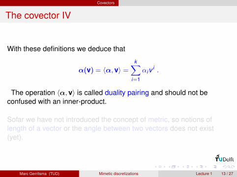
With these definitions we deduce that
α(v) = 〈α,v〉 =k∑
i=1
αiv i .
The operation 〈α,v〉 is called duality pairing and should not beconfused with an inner-product.
Sofar we have not introduced the concept of metric, so notions oflength of a vector or the angle between two vectors does not exist(yet).
Marc Gerritsma (TUD) Mimetic discretizations Lecture 1 13 / 27
Covectors
The covector IV
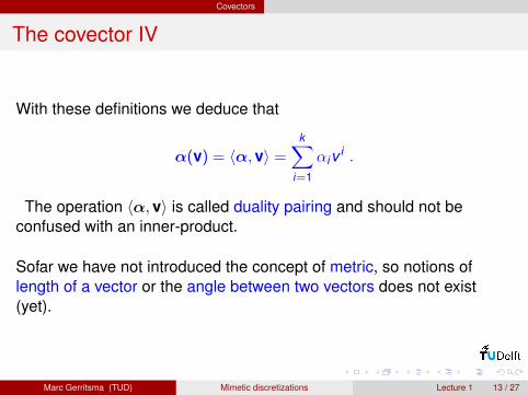
With these definitions we deduce that
α(v) = 〈α,v〉 =k∑
i=1
αiv i .
The operation 〈α,v〉 is called duality pairing and should not beconfused with an inner-product.
Sofar we have not introduced the concept of metric, so notions oflength of a vector or the angle between two vectors does not exist(yet).
Marc Gerritsma (TUD) Mimetic discretizations Lecture 1 13 / 27
Covectors
The covector IV
With these definitions we deduce that
α(v) = 〈α,v〉 =k∑
i=1
αiv i .
The operation 〈α,v〉 is called duality pairing and should not beconfused with an inner-product.
Sofar we have not introduced the concept of metric, so notions oflength of a vector or the angle between two vectors does not exist(yet).
Marc Gerritsma (TUD) Mimetic discretizations Lecture 1 13 / 27
Covectors
Vector and covector fields
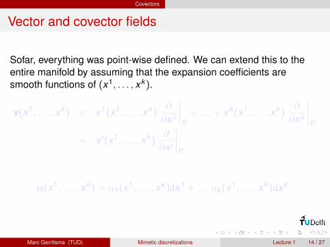
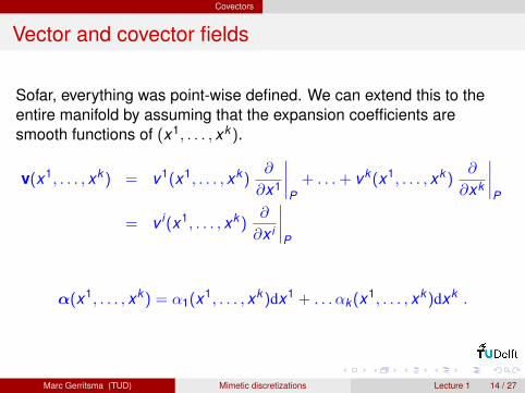
Sofar, everything was point-wise defined. We can extend this to theentire manifold by assuming that the expansion coefficients aresmooth functions of (x1, . . . , xk ).
v(x1, . . . , xk ) = v1(x1, . . . , xk )∂
∂x1
∣∣∣∣P
+ . . .+ vk (x1, . . . , xk )∂
∂xk
∣∣∣∣P
= v i(x1, . . . , xk )∂
∂x i
∣∣∣∣P
α(x1, . . . , xk ) = α1(x1, . . . , xk )dx1 + . . . αk (x1, . . . , xk )dxk .
Marc Gerritsma (TUD) Mimetic discretizations Lecture 1 14 / 27

Covectors
Vector and covector fields
Sofar, everything was point-wise defined. We can extend this to theentire manifold by assuming that the expansion coefficients aresmooth functions of (x1, . . . , xk ).
v(x1, . . . , xk ) = v1(x1, . . . , xk )∂
∂x1
∣∣∣∣P
+ . . .+ vk (x1, . . . , xk )∂
∂xk
∣∣∣∣P
= v i(x1, . . . , xk )∂
∂x i
∣∣∣∣P
α(x1, . . . , xk ) = α1(x1, . . . , xk )dx1 + . . . αk (x1, . . . , xk )dxk .
Marc Gerritsma (TUD) Mimetic discretizations Lecture 1 14 / 27

Wedge product
The wedge product
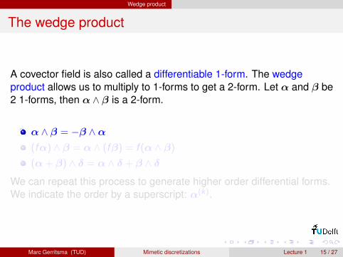
A covector field is also called a differentiable 1-form. The wedgeproduct allows us to multiply to 1-forms to get a 2-form. Let α and β be2 1-forms, then α ∧ β is a 2-form.
α ∧ β = −β ∧α(fα) ∧ β = α ∧ (fβ) = f (α ∧ β)
(α+ β) ∧ δ = α ∧ δ + β ∧ δ
We can repeat this process to generate higher order differential forms.We indicate the order by a superscript: α(k).
Marc Gerritsma (TUD) Mimetic discretizations Lecture 1 15 / 27
Wedge product
The wedge product
A covector field is also called a differentiable 1-form. The wedgeproduct allows us to multiply to 1-forms to get a 2-form. Let α and β be2 1-forms, then α ∧ β is a 2-form.
α ∧ β = −β ∧α(fα) ∧ β = α ∧ (fβ) = f (α ∧ β)
(α+ β) ∧ δ = α ∧ δ + β ∧ δ
We can repeat this process to generate higher order differential forms.We indicate the order by a superscript: α(k).
Marc Gerritsma (TUD) Mimetic discretizations Lecture 1 15 / 27

Differential k -forms
Example I
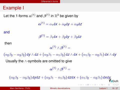
Let the 1-forms α(1) and β(1) in R3 be given by
α(1) = α1dx + α2dy + α3dz
andβ(1) = β1dx + β2dy + β3dz
thenα(1) ∧ β(1) =
(α2β3 − α3β2) dy ∧ dz + (α3β1 − α1β3) dz ∧ dx + (α1β2 − α2β1) dx ∧ dy
Usually the ∧-symbols are omitted to give
α(1) ∧ β(1) =
(α2β3 − α3β2) dydz + (α3β1 − α1β3) dzdx + (α1β2 − α2β1) dxdy
Marc Gerritsma (TUD) Mimetic discretizations Lecture 1 16 / 27
Differential k -forms
Example I
Let the 1-forms α(1) and β(1) in R3 be given by
α(1) = α1dx + α2dy + α3dz
andβ(1) = β1dx + β2dy + β3dz
thenα(1) ∧ β(1) =
(α2β3 − α3β2) dy ∧ dz + (α3β1 − α1β3) dz ∧ dx + (α1β2 − α2β1) dx ∧ dy
Usually the ∧-symbols are omitted to give
α(1) ∧ β(1) =
(α2β3 − α3β2) dydz + (α3β1 − α1β3) dzdx + (α1β2 − α2β1) dxdy
Marc Gerritsma (TUD) Mimetic discretizations Lecture 1 16 / 27

Differential k -forms
Example II
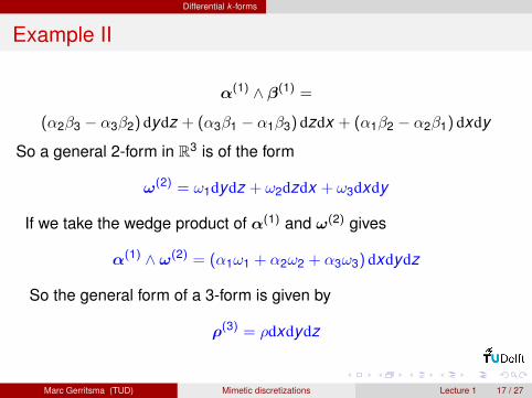
α(1) ∧ β(1) =
(α2β3 − α3β2) dydz + (α3β1 − α1β3) dzdx + (α1β2 − α2β1) dxdy
So a general 2-form in R3 is of the form
ω(2) = ω1dydz + ω2dzdx + ω3dxdy
If we take the wedge product of α(1) and ω(2) gives
α(1) ∧ ω(2) = (α1ω1 + α2ω2 + α3ω3) dxdydz
So the general form of a 3-form is given by
ρ(3) = ρdxdydz
Marc Gerritsma (TUD) Mimetic discretizations Lecture 1 17 / 27

Differential k -forms
Example II
α(1) ∧ β(1) =
(α2β3 − α3β2) dydz + (α3β1 − α1β3) dzdx + (α1β2 − α2β1) dxdy
So a general 2-form in R3 is of the form
ω(2) = ω1dydz + ω2dzdx + ω3dxdy
If we take the wedge product of α(1) and ω(2) gives
α(1) ∧ ω(2) = (α1ω1 + α2ω2 + α3ω3) dxdydz
So the general form of a 3-form is given by
ρ(3) = ρdxdydz
Marc Gerritsma (TUD) Mimetic discretizations Lecture 1 17 / 27
Differential k -forms
Space of k -forms
k -forms on the manifoldM, form a linear vector space denoted byΛk (M). The wedge product is then a map
∧ : Λk (M)× Λl(M)→ Λk+l(M) .
Marc Gerritsma (TUD) Mimetic discretizations Lecture 1 18 / 27

Differential k -forms
Example III
Summary:A 0-form (a function) : f (0) = f (x , y , z)
A 1-form : u(1) = u dx + v dy + w dxA 2-form : ω(2) = ω1 dydz + ω2 dzdx + ω3 dxdyA 3-form : ρ(3) = ρdxdydz
Marc Gerritsma (TUD) Mimetic discretizations Lecture 1 19 / 27
Differential k -forms
Example III
Summary:A 0-form (a function) : f (0) = f (x , y , z)
A 1-form : u(1) = u dx + v dy + w dxA 2-form : ω(2) = ω1 dydz + ω2 dzdx + ω3 dxdyA 3-form : ρ(3) = ρdxdydz
Marc Gerritsma (TUD) Mimetic discretizations Lecture 1 19 / 27

Differential k -forms
Example III
Summary:A 0-form (a function) : f (0) = f (x , y , z)
A 1-form : u(1) = u dx + v dy + w dxA 2-form : ω(2) = ω1 dydz + ω2 dzdx + ω3 dxdyA 3-form : ρ(3) = ρdxdydz
Marc Gerritsma (TUD) Mimetic discretizations Lecture 1 19 / 27
Differential k -forms
Example III
Summary:A 0-form (a function) : f (0) = f (x , y , z)
A 1-form : u(1) = u dx + v dy + w dxA 2-form : ω(2) = ω1 dydz + ω2 dzdx + ω3 dxdyA 3-form : ρ(3) = ρdxdydz
Marc Gerritsma (TUD) Mimetic discretizations Lecture 1 19 / 27

Differential k -forms
Example III
Summary:A 0-form (a function) : f (0) = f (x , y , z)
A 1-form : u(1) = u dx + v dy + w dxA 2-form : ω(2) = ω1 dydz + ω2 dzdx + ω3 dxdyA 3-form : ρ(3) = ρdxdydz
Marc Gerritsma (TUD) Mimetic discretizations Lecture 1 19 / 27

Differential k -forms
Example III
Summary:A 0-form (a function) : f (0) = f (x , y , z)
A 1-form : u(1) = u dx + v dy + w dxA 2-form : ω(2) = ω1 dydz + ω2 dzdx + ω3 dxdyA 3-form : ρ(3) = ρdxdydz
Question: For those new to differential forms, do these expression lookfamiliar to you?
Marc Gerritsma (TUD) Mimetic discretizations Lecture 1 19 / 27

Differential k -forms
Example III
Summary:A 0-form (a function) : f (0) = f (x , y , z)
A 1-form : u(1) = u dx + v dy + w dxA 2-form : ω(2) = ω1 dydz + ω2 dzdx + ω3 dxdyA 3-form : ρ(3) = ρdxdydz
[Flanders, 1963] "These are the things which occur under integralsigns"
Marc Gerritsma (TUD) Mimetic discretizations Lecture 1 19 / 27
Differential k -forms
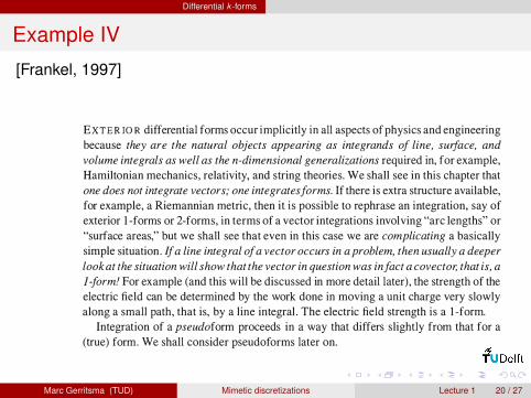
Example IV
[Frankel, 1997]
Marc Gerritsma (TUD) Mimetic discretizations Lecture 1 20 / 27
Integration
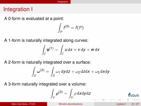
Integration I
A 0-form is evaluated at a point:∫P
f (0) = f (P)
A 1-form is naturally integrated along curves:∫C
u(1) =
∫C
u dx + v dy + w dx
A 2-form is naturally integrated over a surface:∫Sω(2) =
∫Sω1 dydz + ω2 dzdx + ω3 dxdy
A 3-form naturally integrated over a volume:∫Vρ(3) =
∫Vρ dxdydz
Marc Gerritsma (TUD) Mimetic discretizations Lecture 1 21 / 27
Integration
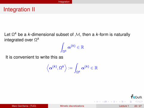
Integration II
Let Ωk be a k -dimensional subset ofM, then a k -form is naturallyintegrated over Ωk ∫
Ωkα(k) ∈ R
It is convenient to write this as⟨α(k),Ωk
⟩:=
∫Ωkα(k) ∈ R
Marc Gerritsma (TUD) Mimetic discretizations Lecture 1 22 / 27
The exterior derivative
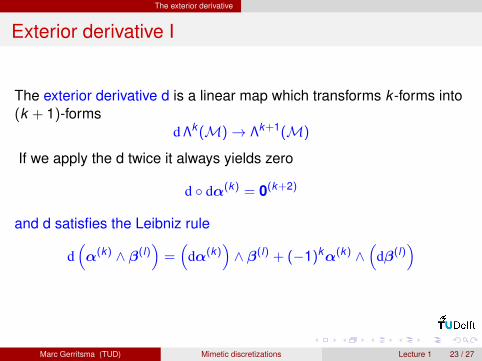
Exterior derivative I
The exterior derivative d is a linear map which transforms k -forms into(k + 1)-forms
d Λk (M)→ Λk+1(M)
If we apply the d twice it always yields zero
d dα(k) = 0(k+2)
and d satisfies the Leibniz rule
d(α(k) ∧ β(l)
)=(
dα(k))∧ β(l) + (−1)kα(k) ∧
(dβ(l)
)
Marc Gerritsma (TUD) Mimetic discretizations Lecture 1 23 / 27
The exterior derivative
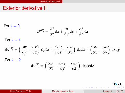
Exterior derivative II
For k = 0df (0) =
∂f∂x
dx +∂f∂y
dy +∂f∂z
dz
For k = 1
du(1) =
(∂w∂y− ∂v∂z
)dydz +
(∂u∂z− ∂w∂x
)dzdx +
(∂v∂x− ∂u∂y
)dxdy
For k = 2
dω(2) =
(∂ω1
∂x+∂ω2
∂y+∂ω3
∂z
)dxdydz
Marc Gerritsma (TUD) Mimetic discretizations Lecture 1 24 / 27

The exterior derivative
Exterior derivative II
For k = 0df (0) =
∂f∂x
dx +∂f∂y
dy +∂f∂z
dz
For k = 1
du(1) =
(∂w∂y− ∂v∂z
)dydz +
(∂u∂z− ∂w∂x
)dzdx +
(∂v∂x− ∂u∂y
)dxdy
For k = 2
dω(2) =
(∂ω1
∂x+∂ω2
∂y+∂ω3
∂z
)dxdydz
Marc Gerritsma (TUD) Mimetic discretizations Lecture 1 24 / 27
The exterior derivative
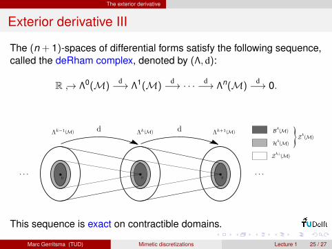
Exterior derivative III
The (n + 1)-spaces of differential forms satisfy the following sequence,called the deRham complex, denoted by (Λ, d):
R → Λ0(M)d−→ Λ1(M)
d−→ · · · d−→ Λn(M)d−→ 0.
H M
B M MMM
Z M,⊥
Z M
This sequence is exact on contractible domains.
Marc Gerritsma (TUD) Mimetic discretizations Lecture 1 25 / 27
The exterior derivative
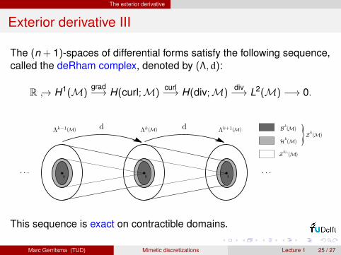
Exterior derivative III
The (n + 1)-spaces of differential forms satisfy the following sequence,called the deRham complex, denoted by (Λ, d):
R → H1(M)grad−→ H(curl;M)
curl−→ H(div;M)div−→ L2(M) −→ 0.
H M
B M MMM
Z M,⊥
Z M
This sequence is exact on contractible domains.
Marc Gerritsma (TUD) Mimetic discretizations Lecture 1 25 / 27
Outlook
The title of this lecture
The title of this lecture is:
∂/∂x and dxA new meaning for familiar symbols
Here we interpret ∂/∂x as a basis vector instead of an operator and dxis a basis functional. The is nothing ‘small’ in these two concepts. Nolimits for h→ 0 are involved.
Instead of approximation, we look for representation of these concepts.
Marc Gerritsma (TUD) Mimetic discretizations Lecture 1 26 / 27
Outlook
The next step
Many of the constructions and operations given in this presentationhave a purely discrete analogue.
Manifold←→ grid (cell complex)Differential forms←→ cochainsExterior derivative←→ coboundary operator
We will discuss these discrete concepts tomorrow.
Marc Gerritsma (TUD) Mimetic discretizations Lecture 1 27 / 27