1

ISABE-2015-20220

A Physics Based Methodology for Building Accurate Gas Turbine Performance Models

Joachim Kurzke

GasTurb

Max Feldbauer Weg 5

85221 Dachau

Germany

Abstract Gas turbine performance models are needed for many

purposes. Engine maintenance shops can use them for

investigating incoming engines, planning the extent of

the repair and assessing the post repair performance.

This paper presents a methodology which minimizes

the effort needed to create physic based accurate

models. As an example serves the model of a CFM56-

3 engine which is calibrated with the raw data from a

test cell correlation report.

Nomenclature

A area

CD discharge coefficient

EGT exhaust gas temperature

FHV fuel heating value

LPC fan

HPC high pressure compressor

HPT high pressure turbine

LPT low pressure turbine

Mn Mach number

N spool speed

P total pressure

R gas constant

SFC specific fuel consumption

T total temperature

V flight velocity

VGV variable guide vanes

W air mass flow

WF fuel mass flow

η efficiency

Θ temperature ratio T/Tstd

Subscripts

ACC active clearance control

R reduced

s static conditions

std standard day conditions

2 engine inlet

25 HPC inlet

3 HPC exit

45 LPT inlet

495 LPT vane stage 2

5 LPT exit

8 core nozzle inlet

18 bypass nozzle inlet

Introduction

Each engine must pass the acceptance test after a

maintenance shop visit before it is declared fit for

flight. Performance wise the engine is ok when it has

sufficient EGT margin. The official acceptance test

result contains no statement about the quality of the

engine components. This, however, is of great interest

for the maintenance shop operator. Having a

thermodynamic model of the cycle can be of great help

for analyzing engine component performance.

How to calibrate the model? Should we use the

corrected data from the official test analysis procedure

as model reference? No - it is better to start with the

raw data for two reasons:

1. The official procedure may do more than

correcting to standard day conditions.

Possibly there are terms considering

differences in the engine built standard or

between test cell and aircraft installation etc.

2. So-called facility modifiers are applied to a

few parameters only. Some quantities like

compressor exit temperature and pressure,

for example, are not corrected. The mixture

of facility corrected and uncorrected data is

thermodynamically not consistent.

This paper describes a thermodynamic model of

the CFM56-3 turbofan engine. The model is based on

data from an official test cell correlation report (ref. 1)

which contains the raw data from two engine runs

(2*20 scans), data corrected with the official

procedure and the above mentioned facility modifiers.

Data Check

It is essential to check the data before beginning with

engine modelling work. The pressures measured in the

bellmouth are a very good starting point for this. There

are six total pressures and four wall static pressure

measurements, all showing little scatter. We can

calculate the total to static pressure ratio P2/Ps2 from

the averaged data which in turn yields the bellmouth

Mach number Mn2.

The total temperature T2 is measured with 24

thermocouples in the bellmouth. One would expect

that the average value of all the measurements agrees

2

with the temperature Tamb which is measured

somewhere in the test cell, however, this is not the

case. The difference between Tamb and T2 increases

with bellmouth Mach number from 0.5K (Mn2=0.3) to

2 K (Mn2=0.68).

The explanation: the T2 probes do not indicate the

true temperature. This is quite normal for total

temperature probes. The recovery factor r describes

the difference between the indicated total temperature

and true total temperature:

𝑟 =𝑇𝑖𝑛𝑑 − 𝑇𝑠

𝑇𝑡𝑟𝑢𝑒 − 𝑇𝑠

(1)

Let us assume that Tamb (measured with a single

probe in the test cell) indicates the true total

temperature of the incoming air. We can calculate the

static temperature Ts from the already determined

bellmouth Mach number and Tamb = T2,rue. Thus we can

determine the recovery coefficient r for each of the

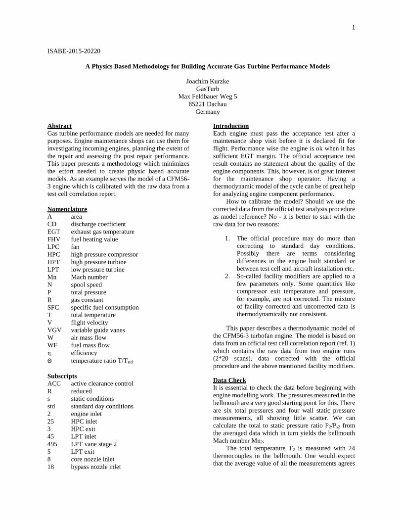
scans - the results are shown in Fig. 1.

Fig. 1: Recovery factor for the bellmouth T2 probes

The scatter between the crosses is remarkably

low which indicates highly accurate raw data. On

average the recovery factor is 0.91. We apply this

average recovery factor r=0.91 to the indicated total

temperature of the probes in the bellmouth. Thus we

get an accurate value for T2 as the basis for the data

correction to standard day conditions.

P2 is measured with four bellmouth rakes each

reading six total pressures. P2 is lower than the ambient

pressure measured at the wall of the test cell, upstream

of the engine. The pressure ratio P2/Pamb correlates

well with bellmouth Mach number, and the scatter in

the data is extremely small,

Mass Flow The mass flow is calculated from the raw data for P2,

the recovery corrected T2, the bellmouth area and the

bellmouth flow coefficient. The latter is given in the

Engine Shop Manual (Ref.2). The standard day

corrected mass flow W2Rstd is highly accurate since all

the input data for the mass flow calculation show very

little scatter.

Thrust The thrust measured at the engine cradle is not the

same as one would measure in an open air test. The

thrust difference depends on the size and the design of

the test cell. Therefore each test cell is calibrated and

the ratio of free stream thrust to measured thrust - the

facility modifier for thrust - is determined.

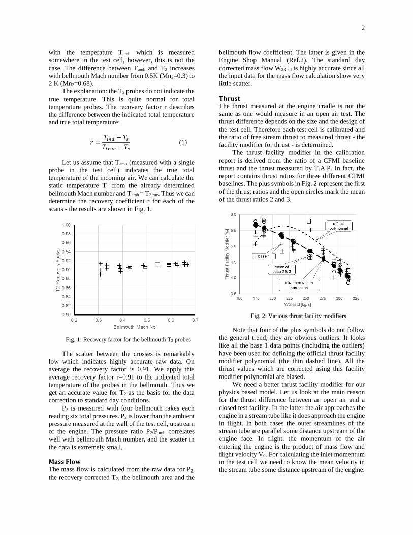
The thrust facility modifier in the calibration

report is derived from the ratio of a CFMI baseline

thrust and the thrust measured by T.A.P. In fact, the

report contains thrust ratios for three different CFMI

baselines. The plus symbols in Fig. 2 represent the first

of the thrust ratios and the open circles mark the mean

of the thrust ratios 2 and 3.

Fig. 2: Various thrust facility modifiers

Note that four of the plus symbols do not follow

the general trend, they are obvious outliers. It looks

like all the base 1 data points (including the outliers)

have been used for defining the official thrust facility

modifier polynomial (the thin dashed line). All the

thrust values which are corrected using this facility

modifier polynomial are biased.

We need a better thrust facility modifier for our

physics based model. Let us look at the main reason

for the thrust difference between an open air and a

closed test facility. In the latter the air approaches the

engine in a stream tube like it does approach the engine

in flight. In both cases the outer streamlines of the

stream tube are parallel some distance upstream of the

engine face. In flight, the momentum of the air

entering the engine is the product of mass flow and

flight velocity V0. For calculating the inlet momentum

in the test cell we need to know the mean velocity in

the stream tube some distance upstream of the engine.

3

How can we determine the representative stream

tube diameter which gives consistent results with the

data from the correlation report? Actually this is easy:

we adjust the stream tube cross-section in such a way

that the momentum based thrust correction agrees with

the mean value from the other three corrections. This

procedure yields a stream tube diameter of 6m for

W2Rstd=310kg/s which decreases slightly to 5.8m when

W2Rstd=170kg/s.

These numbers look plausible: the test cell is

8.65m high and 9.75m wide. There is room left for the

secondary air which bypasses the engine and joins the

exhaust gases in the detuner at the test section exit.

The scatter in the calculated inlet momentum is

very small since the mass flow is determined

accurately from the measurements in the bellmouth.

Therefore the inlet momentum based thrust modifier is

also very accurate as can be seen from Fig. 2. It is a

much better representation of physics than the official

polynomial. The procedure based on the inlet

momentum calculation can be applied with confidence

also outside the calibration range of the test facility.

Fuel Flow Understanding the fuel flow measurement is very

important. The first step of the test analysis is the

correction to standard day conditions and to the

nominal fuel heating value FHVnom:

𝑊𝐹𝑅 =𝑊𝐹𝑚𝑒𝑎𝑠

𝛿 ∗ 𝜃0.68∗ √

𝑅𝑑𝑟𝑦 𝑎𝑖𝑟

𝑅∗

𝐹𝐻𝑉

𝐹𝐻𝑉𝑛𝑜𝑚

(2)

The official procedure as described in Ref. 2

employs additional terms in the equation: an inlet

condensation correction factor (not applicable for the

test conditions), a fuel flow facility modifier and a

correction for the HPT active clearance control. Fig. 3

compares WFR as determined by T.A.P. following the

official procedure with WFR as calculated with

equation 2. The differences - expressed in % - are

generally small and very consistent, except for the two

red points marked A and B which deviate 1%

respectively 0.25% from the general trend. What is the

reason for this abnormality?

It is connected with the HPT active clearance

control of the CFM56 engine. The control valve of the

ACC cooling air has two inlet ports, one from the 5th

and one from the 9th stage of the HP compressor. The

engine control unit decides which of the air supplies is

used - it can also be a mixture of 5th and 9th stage air.

A nominal cooling air mode schedule for operating the

HPT clearance control valve is part of the official test

analysis procedure. In this nominal schedule the valve

position changes at NHR= 13200rpm from stage 5 air

to a mixture of 5th and 9th stage air. Above

NHR=13760rpm all air is taken from the 9th stage.

Near to the switch points in the schedule it can

happen, that the valve is not in its nominal position. In

such a case the measured fuel flow is adjusted for the

deviation of the HPT ACC valve position from the

nominal schedule. Now have a look at the upper part

of Fig. 3 which shows the temperature of the shroud

cooling air downstream of the valve, normalized with

T3. There are two steps in the TACC/T3 data which

indicate that the valve position has changed. It is

conspicuous that W2Rstd of the TACC/T3 steps coincides

with the corrected flows of the points A and B.

Fig. 3: Corrected fuel flow and temperature of the

HPT ACC air

It is quite clear that the official test analysis

procedure has erroneously adjusted the measured fuel

flow of point A by +1% and that of point B by +0.25%.

When these two adjustments are removed, then points

A and B agree perfectly with the other data.

Fig. 3 shows a trend in the fuel flow difference

with W2Rstd. This trend and its magnitude is also seen

in a table of the calibration report which compares the

flowmeters of T.A.P. and SNECMA. We could use

this knowledge for defining a fuel flow facility

modifier. However, we do not know the absolute

accuracy of either flowmeters and therefore we use the

result of equation 2 for the modelling work without

applying a facility modifier to WFR.

Specific fuel consumption– the quotient of fuel

flow and thrust – is a very sensitive measure of overall

engine efficiency. The difference between

thermodynamic (true) and contractual performance in

Fig. 4 is remarkable. The distinct step in SFC at 53kN

thrust which is seen in the thermodynamic

performance analysis is in the results of the official

procedure nearly invisible. The true behavior of the

4

engine is masked by the application of the facility

modifiers and the peculiar HPT clearance corrections.

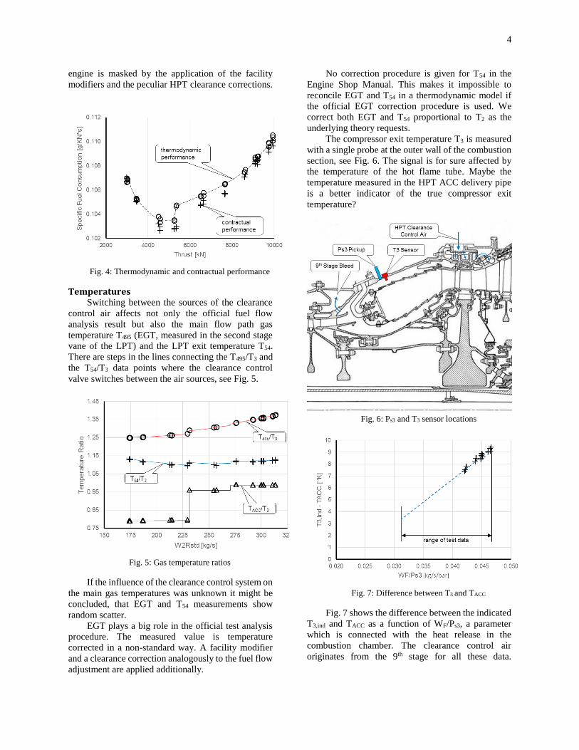
Fig. 4: Thermodynamic and contractual performance

Temperatures Switching between the sources of the clearance

control air affects not only the official fuel flow

analysis result but also the main flow path gas

temperature T495 (EGT, measured in the second stage

vane of the LPT) and the LPT exit temperature T54.

There are steps in the lines connecting the T495/T3 and

the T54/T3 data points where the clearance control

valve switches between the air sources, see Fig. 5.

Fig. 5: Gas temperature ratios

If the influence of the clearance control system on

the main gas temperatures was unknown it might be

concluded, that EGT and T54 measurements show

random scatter.

EGT plays a big role in the official test analysis

procedure. The measured value is temperature

corrected in a non-standard way. A facility modifier

and a clearance correction analogously to the fuel flow

adjustment are applied additionally.

No correction procedure is given for T54 in the

Engine Shop Manual. This makes it impossible to

reconcile EGT and T54 in a thermodynamic model if

the official EGT correction procedure is used. We

correct both EGT and T54 proportional to T2 as the

underlying theory requests.

The compressor exit temperature T3 is measured

with a single probe at the outer wall of the combustion

section, see Fig. 6. The signal is for sure affected by

the temperature of the hot flame tube. Maybe the

temperature measured in the HPT ACC delivery pipe

is a better indicator of the true compressor exit

temperature?

Fig. 6: Ps3 and T3 sensor locations

Fig. 7: Difference between T3 and TACC

Fig. 7 shows the difference between the indicated

T3,ind and TACC as a function of WF/Ps3, a parameter

which is connected with the heat release in the

combustion chamber. The clearance control air

originates from the 9th stage for all these data.

5

Interpreting TACC as the true compressor delivery

temperature is plausible.

Of course TACC cannot be used as the true T3

indicator while part or all of the clearance control air

is taken from the 5th stage. We use for these cases the

linear correlation between (T3,ind - TACC) and WF/Ps3

(the dashed line in Fig. 7) for correcting T3,ind to the

true compressor exit temperature T3.

Two T54 probes measure the temperature

downstream of the LPT. The difference between the

two T54 signals is significant – see Fig. 8. Note that

scans at the same W2Rstd lead to very similar results.

The temperature differences are not random, they have

a reason: The circumferential temperature distribution

changes obviously with W2Rstd.

Fig. 8: Temperature differences at LPT exit

Pressures and Spool Speeds All pressure probes in the engine indicate total

pressures except Ps3 which is a static pressure

measured at the combustion chamber wall, see Fig. 6.

The ratio between total pressure at the compressor exit

P3 and Ps3 remains constant within the tested

operating range because the Mach number at this

location is low and fairly constant. No abnormality

was found in plots of pressure ratios and spool speeds

over corrected flow W2Rstd.

Cycle Reference Point

All calculations for this paper are performed with the

cycle code GasTurb which was written by the author.

The engine modelling work begins with the

reproduction of the measured data from a single scan,

the cycle reference point. Neither component maps nor

speed values are needed for this sort of calculation.

The cycle reference point reproduces the known data

for the parameters listed in table 1.

The simulation of EGT is a peculiarity in case of

the CFM56-3 engine because the measurement is

located within the LPT, at the inlet of the 2nd LPT

rotor. There the mean total temperature is

approximately

𝑇451 = 𝑇45 − 0.217 ∗ (𝑇45 − 𝑇5) (3)

Table 1: Given data

CFMI Name Comment

FN Net thrust = measured force, inlet

momentum corrected (fig. 4)

W2 From bellmouth measurements

WF Corrected with equation 2 to

FHVnom=42.769 MJ/kg

T25 Calculated value:

T25-T2=f(NLR) as defined in the

Engine Shop Manual

T3 Corrected for sensor position to

TACC, see fig. 7

T495 EGT harness in LPT second stage

vane

T5 2 single element rakes

P3/P2 Assumption: Ps3/P3=0.97

P25/P2 single element rake

P5 2 single element rakes

P18/P2 4 rakes, each reading 6 pressures

A8 Core nozzle throat area

A18 Bypass nozzle throat area

The value 0.217 is a guess for the relative

temperature decrease within the four stage LPT due to

work extraction in the 1st rotor. This number is based

on the assumption, that the aerodynamic loading

ΔH/u² of all stages is the same. Note that the

temperature drop in the first stage is less than the

average value of 0.25 because the mean rotor blade

diameter of this stage is the smallest.

Fig. 9: EGT measurement in CFM56-3 engines

6

The indicated EGT (T495) is 1058K, while

equation 3 yields T451= 1084K. The difference of 26K

cannot be explained with an inaccurate T5 signal or

with a wrong assumption about the work distribution

between the LPT stages.

Let us have a closer look at how T495 is measured.

As can be seen in Fig. 9 the thermocouple tip is not

heading in direction of the main gas flow. The gas

whose temperature is measured comes from four holes

in the pressure side of the vane. It is quite certain that

the dynamic head of the gas flowing over the

thermocouple tip is much less than that in the main

stream. Consequently, the recovery factor of the T495

measuring arrangement will be much lower than 1.

To estimate an order of magnitude let us assume

Mach number 0.6 in the main stream. This goes along

with a temperature difference between total and static

temperature of around 55K. The temperature

difference we are looking for is half of that.

These thoughts lead to the following equation for

the EGT signal:

𝑇495 = 0.976 ∗ [𝑇45 − 0.217 ∗ (𝑇45 − 𝑇5)] (4)

The known data do not lead to a unique solution

for the cycle reference point. Slightly different

assumptions about the secondary air system, external

gearbox losses (HP spool mechanical efficiency) duct

losses and nozzle discharge coefficients would lead to

other cycle data.

Off-Design

We have selected one of the operating points as cycle

reference point. We could have selected a different

operating point, so what is special with the cycle

reference point? It is the anchor point for our off-

design model.

In the cycle reference point calculations the

compressor pressure ratios and efficiencies as well as

the turbine efficiencies are given data. During off-

design simulations these data are read from

compressor and turbine maps. The calculation

processes are different, however, at the cycle reference

point both algorithms yield exactly the same result.

Since the true component maps are not available,

we have to use maps from open literature. At the cycle

reference point we scale the compressor and turbine

maps in such a way that reading them at the operating

conditions of the cycle reference point yields both for

the design and off-design calculation processes

exactly the same result.

The off-design calculation at other operating

conditions will initially not match the given data. We

have to tweak the maps until the simulation agrees

with the test results.

Fig. 10 Fan map with operating line

Fan Map

The GasTurb Standard Map is suited as a starting point

for the CFM56-3 model calibration process because it

is from a similar fan (Ref. 3). The question is: where

in this map should we place the cycle reference point?

There are no strict rules, only rough guide lines:

The corrected flow (the x-axis value) is connected

with the Mach number at the fan face. At our cycle

reference point this is calculated as 0.57 from the

fan dimensions and the corrected flow. Setting the

map scaling point to a corrected flow value of 0.9

in the unscaled map implies that for N/√Θ=1.1 the

fan face Mach number is 0.78. This is certainly a

high value which should not be exceeded.

The efficiency at the cycle reference point has a

value which remains unchanged during the map

scaling process. Placing the map scaling point in

a low efficiency region of the unscaled map can

create unrealistically high values in the peak

efficiency region.

With respect to surge margin there is some

freedom. The fan operating line at cruise certainly

passes through the map region where efficiency is

highest. The sea level operating line has less surge

margin due to the lower bypass nozzle pressure

ratio. When we place the map scaling point

slightly above the high efficiency region, then the

cruise operating line will be optimally positioned.

Booster Map

The first attempt to model the booster operating line is

with the GasTurb Standard Map. Fig. 11 shows that

the operating line does not pass through the given data

points. Why is that?

7

Fig. 11: Booster operating line with the GasTurb

Standard booster map

The GasTurb Standard map is seemingly from a

compressor which was designed for a higher Mach

number. We can conclude this both from the shape of

the efficiency islands and the mass flow ranges at high

corrected speeds. The region with high efficiency

values is in a transonic compressor at high corrected

speed nearer to the surge line and there the speed lines

are very steep or even vertical.

The Mach number level in the CFM56-3 booster

is - due to the low circumferential speed - very low.

The map of such a subsonic compressor looks very

different, see Fig. 12.

Fig. 12: Booster operating line in the map of a

subsonic compressor map

This map is a scaled version of the one published

in Ref. 4. The title of this paper is somewhat

misleading: it describes the test vehicle as a high speed

compressor. Actually, the maximum rotor Mach

number at the design point is only 0.8285 – clearly a

subsonic compressor. The highly loaded three stage

compressor has a pressure ratio of 2.4. At our cycle

reference point the CFM56-3 booster pressure ratio is

2.18. Thus the map from Ref. 4 is very well suited for

our purposes.

Fig. 13 Booster map comparison

Fig. 13 compares the two maps. The operating

line passes in both maps through the cycle reference

point. The bold operating line is the one from Fig. 12

while the dotted line is a copy from Fig. 11.

The operating point found with the GasTurb

Standard map for the relative speed 0.93 shows a

significantly higher pressure ratio. That is because the

gray speed line of the transonic compressor is much

steeper than the equivalent speed line of the subsonic

compressor. Note that the shape of the speed lines

becomes similar at lower speeds and the pressure ratio

differences decrease.

HPC Map

The GasTurb Standard map is from a compressor with

variable guide vanes. It is very well suited as a starting

point for the CFM56-3 model calibration. Fig. 14

shows the operating line in the HPC map.

Fig. 14: HP compressor map

HPT Map

The pressure ratio of the CFM56-3 HP turbine is

constant as it is in any gas generator turbine. Corrected

speed NH/√Θ4 varies only a little bit. The operating line

is very short and that’s why reading the HPT map

8

yields always nearly the same efficiency. Therefore

the shape of the efficiency islands in the map does not

influence the simulation accuracy.

LPT Map The LPT operating line in its map is much longer than

that of the HPT. Efficiency changes with pressure ratio

and corrected speed NL/√Θ45 and therefore the shape

of the map matters. As a starting point for the model

calibration we can use GasTurb Standard map.

In case of a low pressure turbine the efficiency is

not the only topic of interest. The change of corrected

flow W45Rstd along the operating line affects the

position of the HPC operating line. Decreasing W45Rstd

at constant NH/√Θ25 not only increases HPC pressure

ratio but also all temperatures in the hot end of the

engine. The shape of the function W45Rstd=f (P45/P5) is

the key to a good simulation of EGT and T5.

Fig. 15 LP turbine map

Fig. 15 shows besides the efficiency islands also

lines for constant corrected flow W45Rstd. At the low

power end of the operating line W45Rstd is only 3%

smaller than at high power. With the GasTurb

Standard map one gets more than 5% flow reduction

along the operating line. The simulated EGT is with

this map 20K higher than measured at the low power

end.

Preliminary Model Calibration

We did select from our library the best suitable

compressor and turbine maps and scaled them such

that they reproduce the cycle reference point

performance at the respective map scaling point.

Running this model for an arbitrary off-design

condition will not yield perfect agreement with the

given data because the efficiency slope and the speed-

flow correlation along the operating line differ from

reality. We will get that right next.

Booster Efficiency

Let us begin with the booster map which includes the

fan root performance. It is easy to adapt efficiency

along the operating line: We shift in the map tables all

efficiency values on each speed up or down until the

efficiency on the operating line agrees with the given

value.

HPC Efficiency

Adapting the map of the HPC to the measured data is

a similar process as in case of the booster. We shift the

efficiency values in the map table up and down as

required.

Fig. 16: Nozzle discharge coefficient derived from the

measure data

Bypass Ratio

Before we go for the fan efficiency we make sure that

we are on the right fan operating line which is given

by the measured values of mass flow and fan pressure

ratio. We can achieve this with an appropriate

correlation between the bypass nozzle discharge

coefficient CD18 and bypass nozzle pressure ratio

P18/Pamb.

After having adjusted the fan operating line we

know the bypass ratio and can calculate the core exit

mass flow W5. Among the measured values are LPT

exit pressure P5 and temperature T5. Thus we know the

core nozzle entry conditions and we can calculate the

discharge coefficient CD8 for each of the data points.

For our model we use the correlation between CD8 and

core nozzle pressure ratio P8/Pamb from Fig. 16

Fan and LPT Efficiency Efficiencies along the operating lines of booster and

HPC are in line with the measured data. HPT

efficiency is nearly constant. These three components

are modeled correctly. There are only two properties

9

left for adjusting the simulation to the measured SFC

values: The efficiencies of the fan and the LPT. Both

affect SFC in a similar way as can be seen in Fig. 17.

Fig. 17: Trends for SFC=11.5g/(kN*s) @ FN=60kN

The middle line shows that a change of ΔηLPT

from -2% to +2% requires a change of ΔηLPC from

+2.7% to -2.7% for keeping SFC constant. We could

decide to improve at 60kN the fan efficiency

somewhat, but then we would have to decrease LPT

efficiency accordingly.

In our model both the LPC and the LPT

efficiency drop along the operating line (Fig. 10 and

Fig. 15) by approximately the same amount. This

balance seems to be a reasonable assumption.

Spool Speeds

Getting spool speeds right is the last step of the model

calibration process. Let us first explain the principle of

the speed calibration methodology in detail.

Any compressor map consists of tables in which

corrected spool speed is a parameter. During the map

scaling process of GasTurb, all speed values in the

map tables are multiplied with a constant factor such

that at the map scaling point the corrected speed is

equal to 1.0. Now all the tabulated speed parameter

values stand for relative corrected spool speed.

Using this map within a thermodynamically

calibrated performance model gives the correct

answers for mass flow, efficiency and pressure ratio.

Only the speed parameter value - which has been used

for reading the map at a given operating point - is not

necessarily correct because in the true map the

correlation between corrected speed and corrected

mass flow might be different. For getting the speed-

flow characteristic right we adjust the speed parameter

values in the map tables.

Low Pressure Spool

Finding the NL model is easy in this case because we

know the fan operating line from the measured values

of W2Rstd and P18/P2. We can run an operating line and

check how much the simulated corrected speed

NL/√Θ2 deviates from the measured one. Correcting

the tabulated speed parameter values such that

agreement with the measured data is achieved is easy.

Next we will get the speed-flow correlation of the

booster right. For that purpose we need to know the

corrected flow W22Rstd. Unfortunately we do not have

measured values for that flow. As a substitute we use

“hybrid measured data” which stem from the model

correlation between W22Rstd and P3/P2. We assign to

each of the measured P3/P2 values a model derived

flow W22Rstd.

Now we can compare the flow W22Rstd read from

the map tables at the measured speed NL/√Θ2 with

W22Rstd derived from the measurement. We can get

agreement between these two flows when we modify

the speed values in the map table accordingly.

High Pressure Spool

For getting the speed-flow correlation in the HPC

right we employ hybrid W25Rstd values and modify the

speed values in the map table as necessary.

Strictly speaking there is no justification for

modifying the speed values in the booster map tables

more than a small amount. In case of the HPC,

however, we can justify bigger changes in the numbers

for speed because the HPC has VGV’s.

We do not know the VGV schedule for which the

un-scaled HPC map is valid. For sure the VGV

schedule of the CFM56-3 is different. That is the main

reason why the speed-flow correlation needs

adjustment.

Model Check

Now let us compare the quality of our preliminary

model with the measured data. We have three

important criteria:

1. The so-called SFC loop which is a measure

of thermal efficiency (Fig. 18).

2. Accuracy of the exhaust gas temperature

EGT

3. Accuracy of the LPT exit temperature T5

The simulated SFC agrees well with the

measurements for thrust above 53kN thrust. This is no

wonder: we have adapted fan and LPT efficiency such

that the model matches the measured values in the high

thrust range. The simulated SFC at low thrust is

significantly higher than measured.

Of course we could have adjusted fan and LPT

efficiencies differently to get the “compromise model”

SFC loop. With such an approach we would implicitly

assume that the SFC step at W2Rstd=230kg/s is a

random effect caused by measurement noise.

10

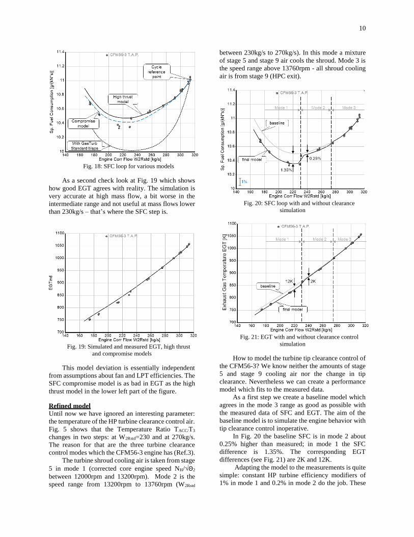
Fig. 18: SFC loop for various models

As a second check look at Fig. 19 which shows

how good EGT agrees with reality. The simulation is

very accurate at high mass flow, a bit worse in the

intermediate range and not useful at mass flows lower

than 230kg/s – that’s where the SFC step is.

Fig. 19: Simulated and measured EGT, high thrust

and compromise models

This model deviation is essentially independent

from assumptions about fan and LPT efficiencies. The

SFC compromise model is as bad in EGT as the high

thrust model in the lower left part of the figure.

Refined model

Until now we have ignored an interesting parameter:

the temperature of the HP turbine clearance control air.

Fig. 5 shows that the Temperature Ratio TACC/T3

changes in two steps: at W2Rstd=230 and at 270kg/s.

The reason for that are the three turbine clearance

control modes which the CFM56-3 engine has (Ref.3).

The turbine shroud cooling air is taken from stage

5 in mode 1 (corrected core engine speed NH/√Θ2

between 12000rpm and 13200rpm). Mode 2 is the

speed range from 13200rpm to 13760rpm (W2Rstd

between 230kg/s to 270kg/s). In this mode a mixture

of stage 5 and stage 9 air cools the shroud. Mode 3 is

the speed range above 13760rpm - all shroud cooling

air is from stage 9 (HPC exit).

Fig. 20: SFC loop with and without clearance

simulation

Fig. 21: EGT with and without clearance control

simulation

How to model the turbine tip clearance control of

the CFM56-3? We know neither the amounts of stage

5 and stage 9 cooling air nor the change in tip

clearance. Nevertheless we can create a performance

model which fits to the measured data.

As a first step we create a baseline model which

agrees in the mode 3 range as good as possible with

the measured data of SFC and EGT. The aim of the

baseline model is to simulate the engine behavior with

tip clearance control inoperative.

In Fig. 20 the baseline SFC is in mode 2 about

0.25% higher than measured; in mode 1 the SFC

difference is 1.35%. The corresponding EGT

differences (see Fig. 21) are 2K and 12K.

Adapting the model to the measurements is quite

simple: constant HP turbine efficiency modifiers of

1% in mode 1 and 0.2% in mode 2 do the job. These

11

modifiers correct simultaneously SFC, EGT and T5

while the other model parameters are nearly not

affected by this model trim.

Fig. 22: The most inaccurate match with the data

The agreement of the final model with the

measurements in Fig. 20 and Fig. 21 is excellent. The

comparison in Fig. 22 does not look so good; actually

the calculated T5 deviates much more than EGT from

the given data. There are good reasons for ignoring

these differences between theory and measurement:

Have again a look at Fig. 8 which shows the

temperature differences between the two only T5

sensors. The mean value of these sensors is certainly

not always representative for the thermodynamic

average as it is predicted by the model.

Fig. 23: One example from many similar correlations

A full check of the model consists of many

figures with all sorts of parameters. Among those are

thrust, mass flows, spool speeds, temperatures and

pressures. Fig. 23 is a typical example, the agreement

between theory and reality is of the same quality in all

the other correlations.

By the way, the operating lines and the maps of

the fan (Fig. 10), the booster (Fig. 12), HPC (Fig. 14)

and LPT (Fig. 15) are those from the final model.

Some Final Remarks

A first look at the SFC loop (Fig. 18) might give the

impression that there is much scatter in the data. One

could make a compromise model and regard the job as

finished. Doing this gives away much of the model

accuracy potential.

It is quite obvious that the 1.2% step in SFC near

to 53kN thrust (W2Rstd≈230kg/s) is not due to random

measurement noise. However, how to consider the

SFC step in the model? If one does not know about the

turbine tip clearance control then one might be

tempted to tweak fan efficiency. The result would be a

distorted fan map which is not justifiable in terms of

compressor physics.

One last advice: Try during model development

many different ideas, however, be aware of too

complex models. When done check whether all the

bells and whistles you might have added are really

necessary. A good model is accurate, based only on

elements you really understand and simple to handle.

References

Ref. 1 CFMI

Correlation Report of TAP Air Portugal for CFM56-3

Engine.

Prepared by P. Compenat and F. Trimouille

Approved by R. Mouginot. October 1991.

Ref. 2 CFMI.

CFM56-3 Engine Shop Manual - Engine Test – Test

003 – Engine Acceptance Test

Task 72-00-00-760-003-0. 2011.

Ref. 3 C. Freeman

Method for the Prediction of Supersonic Compressor

Blade Performance

Journal of Propulsion, Vol 8, No 1, 1992

Ref.4 D. Lippert, G.Woollatt, P.C. Ivey, P. Timmis

and B.A. Charnley

The design, development and evaluation of 3D

Aerofoils for High Speed Axial Compressors

ASME GT2005-68792, 2005

Ref. 5 J. Kurzke

GasTurb 12 Manual

www.gasturb.de

Ref. 6

http://www.air.flyingway.com/books/engineering/CF

M56-3/ctc-142_Line_Maintenance.pdf