A Parsimonious Watershed Model - School of...

1

CHAPTER 22

A Parsimonious Watershed Model

James F. Limbrunner, Richard M. Vogel, and Steven C. Chapra

Department of Civil and Environmental Engineering, Tufts University, Medford, MA 02155, U.S.A.,

email: [email protected], [email protected] and [email protected] ,

Tel: 617-627-3211, FAX: 617-627-3994

1. INTRODUCTION

There are now a very large number of watershed models for predicting streamflow from climatic inputs and land surface characteristics as evidenced by this book, by the 25 watershed models presented in its predecessor (Singh, 1995) and by the 72 models reviewed in Singh and Woolhiser (2002). Alternative temporal and spatial scales are numerous, and watershed modeling philosophies are diverse. The degree of model complexity, as indicated by number of parameters, also varies widely. Beven (1989) suggests that in spite of the dozens of parameters normally included in watershed models, “it appears that 3 to 5 parameters should be sufficient to reproduce most of the information in a hydrologic record.” Jakeman and Hornberger (1993) and others have drawn similar conclusions. A parsimonious watershed model is very careful or economical and even sparing in its use of model parameters.

Most of the watershed models described in this text, in Singh (1995) and in Singh and Woolhiser (2002) have well in excess of 3 to 5 model parameters, many with more than 10-20 model parameters. On the one hand, such models are useful for detailed engineering and scientific studies of watershed processes, yet on the other hand, calibration and uncertainty analyses for such models is much more challenging than for parsimonious models. For example, it can take on the order of weeks to develop a realistic calibration of the HSPF model, whereas a parsimonious model can be calibrated in less than a day. Furthermore, operations such as validation, uncertainty analysis, and extension of complex models to ungaged watersheds using regional calibration methods (see Chapter 3) can be extremely challenging compared to a parsimonious model introduced here.

The daily water balance model presented here is parsimonious in that it has only four adjustable parameters. It combines empiricism and mechanistically based elements, following in the tradition of the U.S. Soil Conservation Service (now Natural Resource Conservation Service) Curve Number (CN) Method (USDA-SCS, 1983, 1986). The model simulates daily variations in evapotranspiration, soil moisture, saturated groundwater, groundwater outflow, snow accumulation, snowmelt and streamflow. Since this model makes so many simplistic assumptions, it gives only a rough approximation to the

2 WATERSHED MODELS

hydrologic behavior of the watershed, and as a result is only intended for planning level studies. On the other hand, its parsimonious nature and its use of the CN method offer many advantages over alternative models as is discussed below. 1.1 The Soil Conservation Service Curve Number Method The Curve Number (CN) Method is an approach based on relationships among rainfall, land characteristics, and streamflow, which developed from empirical investigations on small agricultural watersheds, and appeared in the US Soil Conservation Service’s National Engineering Handbook in the mid-1960s (Mockus, 1972). It was later extended and adapted for use in urban catchments (USDA-SCS, 1983, 1986). It is likely the most widely applied and accepted rainfall-runoff model in engineering practice, due to ease of use, widely available parameter estimation tables, and its incorporation in publicly available software such as TR-20 (USDA-SCS, 1983), TR-55 (USDA-SCS, 1986), HEC-1 (USACE-HEC, 1985), and HEC-1’s later incarnation, HEC-HMS (USACE-HEC, 2000). Note that all of these models are event-based watershed models, whereas the watershed model introduced in this chapter is a continuous daily model.

Perhaps most importantly, the parameter estimation tables for CN enable one to easily determine the impacts of land-use and soil characteristics on runoff in a detailed and comprehensive fashion which is not really comparable to any other existing watershed model. Those extensive and practical tables of CN published in USDA (1986) and many hydrology textbooks and handbooks enable engineers to evaluate detailed hydrologic impacts of various land-development and BMP strategies. In addition to the storm event models cited above, the CN Method has also been incorporated into a variety of continuous hydrologic and water quality simulation models. Tracking of soil moisture and evapotranspiration are common additions to the original event-based CN method that add physically based components to the empiricism inherent in the use of run-off curve numbers. A few examples of continuous simulation models which incorporate the CN method include AnnAGNPS (USDA-ARS-NSL, 2001), EPIC (Williams, 1995), GLEAMS (Knisel and Davis, 2000), GWLF (Haith and Shoemaker, 1987) and SPAW (Chapter 17). The inclusion of the CN method in the variety of event-based and continuous watershed models provides evidence that this approach is pervasive in both hydrologic modeling and non-point source pollution modeling for watersheds. 1.2 Water Balance Models and the Importance of Parsimony While event-based models are sufficient for some flood management problems such as sizing levees, culverts and detention infrastructure, increasingly, continuous simulation is needed for the solution of a wide range of water and environmental engineering problems. For example, continuous

A Parsimonious Watershed Model 3

simulation is required for sizing water supply reservoirs, and hydropower systems, evaluating long term impacts of climate and/or land-use changes, for use in decision support systems and forecast systems and for a variety of sediment and chemical transport problems as described in Chapters 17-19. In this section, we put our “parsimonious watershed model” into context by describing a series of very simple water balance models, along with some of their advantages and distinguishing features. A water balance underlies nearly every watershed model with differences mostly related to the degree of physical representation of sub-processes. The simplest water balance model takes the form. QPET −= (27.1) where long-term average evapotranspiration, ET, is the difference between measured precipitation P and streamflow Q. The next most complex water balance model is probably the ‘abc’ model which was introduced by Fiering (1967) mostly for pedagogic purposes. The ‘abc’ model uses a linear equation with only three parameters to describe a water balance between P, Q, ET, saturated groundwater storage and groundwater outflow. Since it is a linear model, Fiering (1967) and Vogel and Sankarasubramanian (2003) were able to derive generalized relationships between the model parameters and moments of the climatic input, streamflow and model error, enabling one to perform rather advanced uncertainty analyses. The simplicity of the ‘abc’ model has enabled many fundamental applications which are useful for a host of watershed modeling exercises ranging from model calibration, validation, and uncertainty analysis to hypothesis testing (see Vogel and Sankarasubramanian, 2003, for citations to such examples).

The next level of complexity of water balance models are monthly water balance models such as the ‘abcd’ model, Thornthwaite and Mather model and the Palmer model, summarized by Alley (1984) and the hydrologic component of GWLF (Haith and Shoemaker, 1987). Chapter 3, (section 3.2) describes a number of studies, in addition to Alley (1984) which have compared the performance of monthly water balance models. In general, the consensus is that most of the monthly water balance models introduced to the literature perform similarly. The model introduced here is intended as a daily watershed model, although it could also be considered a monthly water balance model, because it is of the same complexity (3-5 parameters) as the monthly water balance models discussed in section 3.2 of Chapter 3. Furthermore, the water balance model introduced here has many advantages over existing monthly water balance models, again, due to its use of the CN method.

Parsimonious models with few parameters are attractive for educational purposes, both for hydrology students and for the public because they are transparent, easy to code, and require minimal input data. While not appropriate for some scientific purposes, they are useful for planning and management studies and they can be quite helpful in communicating technical ideas to non-technical decision makers, allowing them to understand better the natural

4 WATERSHED MODELS

processes which govern the effects of policy decisions such as storm water management schemes or water allocation policies. Since they only require readily available input data, they can be used for screening purposes as an aid to decision making without large expenditures on data collection and technical expertise needed for the creation of more complex models. 1.3 A Parsimonious Model

Four adjustable parameters are used to estimate daily streamflow from climate inputs of average daily temperature and daily precipitation.. The parameters are a coefficient for scaling CN, a snow melt parameter, and two rate parameters used to represent (slow) outflow from groundwater storage and (fast) outflow from stream network storage.

The model introduced here draws heavily upon the hydrologic component of Haith and Shoemaker’s (1987) GWLF model. GWLF is a continuous daily water balance model, that reports only monthly averages, whereas our model reports daily modeled streamflow. GWLF melds the CN method with a simple snow accumulation/melt routine, a soil moisture accounting model and a groundwater accounting model. The GWLF model, which was not included in Singh (1995) or Singh and Woolhiser (2002), has become popular as evidenced by over 50 papers which have cited Haith and Shoemaker’s original article, and the thousands of references one obtains through an internet search. The model described here follows closely from GWLF and is intended for educational and planning level decision problems, such as in the analysis of land use changes or the impacts of watershed management practices on watershed processes.

2. MODEL FORMULATION

2.1 Model Summary Daily streamflow is the sum of direct runoff from precipitation and snow melt events, and groundwater outflow, as in both the ‘abc’ and GWLF models. Evapotranspiration removes water from the basin by acting on water stored in the unsaturated subsurface zone. Equations (27.2) to (27.6) present the complete model in summary form. Each of the model terms are then described in more detail in equations (27.7-27.23). Infiltration to the unsaturated soil zone is the difference between effective precipitation Pe(t) and direct runoff R(t). I(t) = Pe(t) – R(t) (27.2)


Effective precipitation is the sum of rainfall and snowmelt. The continuity equation yields unsaturated zone soil storage S(t) as a recursive function of previous storage, infiltration, percolation Perc(t), and evapotranspiration ET(t). )()()()1()( tETtPerctItStS −−+−= (27.3) Saturated zone groundwater storage G(t) is a function of previous storage, base flow kbG(t-1), and percolation. G(t) = G(t-1) + Perc(t) – kbG(t-1) (27.4) Streamflow Q(t) is defined as the outflow from the network of stream channels, through which baseflow and runoff are routed Q(t) = kN (N(t)+R(t)+G(t)) (27.5) and the network of stream channels has a storage equal to N(t) where N(t+1) = N(t) -Q(t) (27.6) Further detail and definitions are provided in the following sections. 2.2 Direct Runoff R(t) from Land Surfaces Using the CN Method Direct runoff is determined from characteristics of the land surface quantified by CN, as well as precipitation P(t), and antecedent moisture soil conditions. The governing equation for the curve number method is

))()()((

))()(()(

2

tWStItPtItP

tRa

a

+−−

= if P(t) > Ia(t) (27.7)

and zero otherwise, where R(t) is direct runoff at time t, P(t) is precipitation (cm) at time t, WS(t) is watershed soil storage capacity at time t and Ia(t) is an initial abstraction. Watershed soil storage depends on watershed land uses, soil types and antecedent conditions. The initial abstraction includes all initial losses before direct runoff begins and is computed from watershed storage capacity using )(2.0)( tWStIa = (27.8) When snow accumulation and snowmelt are important processes, we replace P(t) in (27.7) with the term effective precipitation Pe(t) described below. Combining (27.7) and (27.8) leads to

6 WATERSHED MODELS

))(8.0)((

))(2.0)(()(2

tWStPtWStPtR

Le

LeL +

−= if Pe(t) > Ia,L(t), else 0. (27.9)

where Pe(t) = P(t) + Ps(t) for T(t) > 0, and 0 otherwise (27.10) where P(t) is rainfall, Ps(t) is snowmelt, and T(t) is average daily temperature in

oC. In equations (27.9), (27.10) and subsequently, subscript “L” has been added to represent variables applied to each land use area in the watershed. The term WSL(t) is a watershed soil storage capacity term (cm) in land use L, which is related to the runoff curve number CN(t) by,

4.25)(

2540)( −=tCN

tWSL

L (27.11)

Curve numbers depend on land-use, soil characteristics, and antecedent moisture conditions. A Curve Number value for ‘normal’ soil moisture conditions is termed CN2 and is either calculated from land use and soil type or adjusted in the calibration process. Since runoff and infiltration characteristics on a soil plot depend on antecedent moisture conditions, the NRCS method adjusts the curve number to a lower value CN1 under dry conditions and a higher value CN3 under wet conditions. Haith et. al (1996) provide the following relationships for curve numbers corresponding to different antecedent moisture conditions:

)01334.0334.2( ,2

,2,1

L

LL CN

CNCN

⋅−= (27.12a)

)0059.04036.0( ,2

,2,3

L

LL CN

CNCN

⋅+= (27.12b)

The curve number is then interpolated between CN1 and CN3 using

LL

LLLL CN

StSCNCNtCN ,1

max,,1,3

)1()()( +−

⋅−= (27.12c)

where S(t) is a state variable representing unsaturated zone soil storage (cm) at time t and Smax is the maximum allowable unsaturated soil storage which is computed from the watershed storage capacity equation in (27.11) using


4.252540

,1max −=

LL CN

S (27.13)

max/)( StS is the unsaturated zone soil moisture content at time t. Now, CN2 is

the model parameter which is adjusted based on land use and soil characteristics, and CN(t) is computed from (27.12). In general, the values of CN(t), CN1, CN2 and CN3 will range from 50 for undeveloped land to nearly 100 for completely impervious surfaces. Extensive tables are available (see USDA, 1986) for estimation of CN2 from soil and land use information. 2.3 Snow

Snow accumulation and melt is based entirely on average daily temperature. When average daily temperature T(t) is below 0oC, any precipitation falling on that day is added to the snow pack, rather than routed through the rainfall-runoff portion of the model.

⎩⎨⎧

−−°≤+−

=otherwise)()1(

0)(if)()1()(

tPtSnowCtTtPtSnow

tSnows

(27.14)

and )()( tTMtPs ⋅= (27.15) with the condition that Snow(t) is non-negative and where Ps(t) represents water melted from the snow pack (cm), T(t) is mean daily temperature in oC, and M is a calibrated model parameter. 2.4 Evapotranspiration

Potential evapotranspiration (PET) is calculated using Hamon’s method (1968) when average air temperature is above 0oC although in principle, any method of estimating PET is possible. Actual evapotranspiration, ET (cm) is calculated by,

)()1(

)(max,

tPETS

tStET

L

LL ⋅

−= (27.16)

where S(t)/Smax is a soil moisture term which reduces ET based on soil dryness and mitigates the tendency for the subsurface to dry completely during long periods without precipitation. This could be conceptualized as a process such as plants wilting, thus reducing transpiration during an extended dry period.

8 WATERSHED MODELS

2.5 Groundwater Hydrology

Infiltration is the vertical transfer of water into the soil moisture compartment of the model. The model does not include surface depression storage, hence infiltration I(t) is simply the difference between effective precipitation Pe(t) and direct runoff R(t), expressed in inches per day: )()()( tRtPtI LeL −= if )()( tRtP Le > (27.17)

Percolation, the transport of water from the soil moisture compartment to groundwater, is computed by first introducing a soil surplus variable SS(t) = S(t-1) + I(t). Then percolation, Perc(t) is computed from

⎩⎨⎧ >−

= otherwise0)(if)()( max,max, LLLL

LStSSStSStPerc (27.18)

Soil moisture storage for each land use, L, is then computed using the continuity equation )()()()1()( tETtPerctItStS LLLLL −−+−= (27.19) where S(t) is unsaturated storage (cm) at beginning of time step t. A sketch of the modeled subsurface hydrology is shown in Figure 2.1. Again, the continuity equation is used to obtain the saturated groundwater storage G(t) as previous saturated groundwater storage plus percolation Perc(t) from above, less groundwater outflow kb G(t) to the stream channel. )1()()1()( −−+−= ∑ tGktPerc

aa

tGtG bL

LT

L (27.20)

where aL is the area covered by land use L, and aT is total watershed area. Thus, aL/aT distributes the depth of percolation from land use L over the entire watershed area. 2.6 Streamflow

Finally, streamflow Q(t) is obtained by routing direct runoff and baseflow through the stream network storage volume, N(t), where

⎥⎦

⎤⎢⎣

⎡−++= ∑

LbL

T

LN tGktR

aatNktQ )1()()()( (27.21)

and )()()1( tQtNtN −=+ (27.22)


The stream network storage volume is envisioned as a store which has groundwater outflow and direct runoff as inputs and streamflow as outputs. Here direct runoff is summed over all land-uses.

Figure 27.1: Subsurface Hydrology Sketch 2.7 Model Parameters The model parameters which normally require adjustment during the calibration process include the following: Rate parameters, kb and kN. The parameter kb is termed the baseflow recession constant. It governs the time release of water from the saturated groundwater store. One can also think of the parameter 1/kb as the average residence time of water in the groundwater zone. One expects the residence time to be in excess of the model time step ∆t = 1 day, hence 1/kb > 1, or 0<kb < 1. The parameter kN represents the inverse of residence time in the stream network and serves as a simple surrogate for routing of streamflow in a channel. Similarly one expects 0 < kN < 1. Also see Figure 27.5 for a graphical approach to estimation of both rate parameters. Runoff Curve Number Scale Factor, B. The value of the runoff curve number, CN2 for use in estimation of CN(t) in equation 27.11c, can be estimated from tables in the TR-55 manual (USDA, 1986). During the calibration process, a scale factor is introduced such that, 55,2,2 −⋅= TRL CNBCN (27.23)

10 WATERSHED MODELS

where B is a constant used to scale all of the CNs obtained from TR-55 tables. This allows for an adjustment of both direct runoff and maximum unsaturated zone soil moisture capacity, while preserving the relative permeability of various land uses with each other, since all CN values are scaled by the same factor. Snow Melt Parameter, M. The snow melt parameter adjusts the sensitivity of snow melt to increased temperature. Plausible values of the model parameter M can be obtained from Table 7.3.7 in Gray and Prowse (1993) keeping in mind appropriate unit conversions. 2.8 Comparison with GWLF

While primarily based on the hydrologic component of GWLF (Haith and Shoemaker, 1987), the parsimonious watershed model described here:

• has a daily time-step unlike GWLF which reports streamflow at a monthly time step.

• interpolates CN(t) as a continuous function ranging from CN1 to CN3 based on the previous day’s soil moisture content, (eqns. 27.12a-c) eliminating the need for GWLF’s wet/dry index calculated from the previous 5-day rainfall;

• links maximum soil moisture storage directly to CN in equation 27.13, eliminating a parameter defined by the user in GWLF;

• uses soil moisture content, S(t-1)/Smax, to scale potential evapotranspiration to actual evapotranspiration by accounting for decreasing plant transpiration under conditions of low soil moisture (eqn. 27.16);

• eliminates the “deep seepage” term; • breaks the unsaturated zone into separate areas according to land use,

each having its own soil moisture content, determined by CN and evapotranspiration.

• adds a simple channel storage routing model (eqn. 27.21) to capture the impact of channel storage processes which may be particularly important for large watersheds.

3. A CASE STUDY

The parsimonious watershed model introduced here was applied to the Aberjona River watershed, a small urbanized catchment of 6,500 hectares located northwest of Boston, Massachusetts. Curve numbers were estimated using digital land use and soil maps. Daily streamflow was obtained from the U.S. Geological Survey and daily temperature and precipitation data were obtained from the National Climate Data Center.


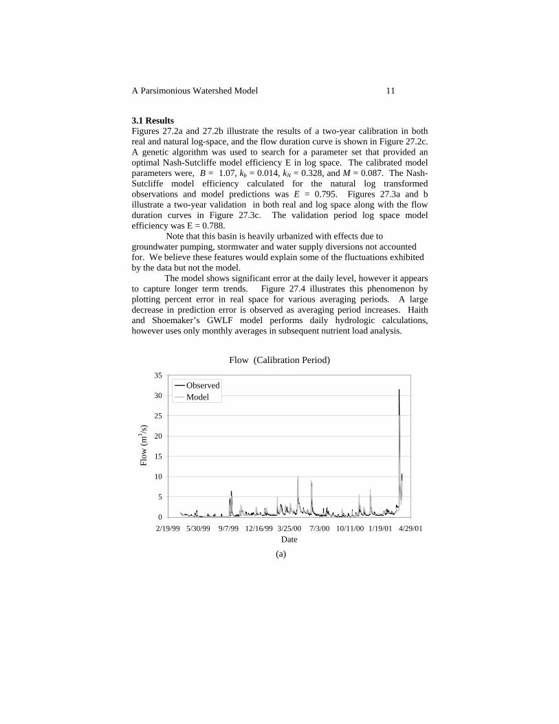
3.1 Results Figures 27.2a and 27.2b illustrate the results of a two-year calibration in both real and natural log-space, and the flow duration curve is shown in Figure 27.2c. A genetic algorithm was used to search for a parameter set that provided an optimal Nash-Sutcliffe model efficiency E in log space. The calibrated model parameters were, B = 1.07, kb = 0.014, kN = 0.328, and M = 0.087. The Nash-Sutcliffe model efficiency calculated for the natural log transformed observations and model predictions was E = 0.795. Figures 27.3a and b illustrate a two-year validation in both real and log space along with the flow duration curves in Figure 27.3c. The validation period log space model efficiency was E = 0.788. Note that this basin is heavily urbanized with effects due to groundwater pumping, stormwater and water supply diversions not accounted for. We believe these features would explain some of the fluctuations exhibited by the data but not the model.

The model shows significant error at the daily level, however it appears to capture longer term trends. Figure 27.4 illustrates this phenomenon by plotting percent error in real space for various averaging periods. A large decrease in prediction error is observed as averaging period increases. Haith and Shoemaker’s GWLF model performs daily hydrologic calculations, however uses only monthly averages in subsequent nutrient load analysis.

Flow (Calibration Period)

0

5

10

15

20

25

30

35

2/19/99 5/30/99 9/7/99 12/16/99 3/25/00 7/3/00 10/11/00 1/19/01 4/29/01Date

Flow

(m3 /s

)

ObservedModel

(a)

12 WATERSHED MODELS

Natural Log-Space Flow (Calibration Period)

-4

-3

-2

-1

0

1

2

3

4

2/19/99 5/30/99 9/7/99 12/16/99 3/25/00 7/3/00 10/11/00 1/19/01 4/29/01Date

Flow

LN

(m3 /s

)ObservedModel

(b)

Log-Space Flow Duration Curve (Calibration Period)

-4

-3

-2

-1

0

1

2

3

4

0 0.2 0.4 0.6 0.8 1Exceedance Probability

Log-

Spac

e Fl

ow

LN(m

3 /s)

ObservedModel

(c)

Figure 27.2 – Calibration of a Parsimonious Watershed Model to the Aberjona River in Massachusetts


Flow (Validation Period)

0

1

2

3

4

5

6

7

8

9

10

2/19/01 5/30/01 9/7/01 12/16/01 3/26/02 7/4/02 10/12/02 1/20/03 4/30/03Date

Flow

(m3 /s

)ObservedModel

(a) .

Natural Log-Space Flow (Validation Period)

-4

-3

-2

-1

0

1

2

3

2/19/01 5/30/01 9/7/01 12/16/01 3/26/02 7/4/02 10/12/02 1/20/03 4/30/03Date

Flow

LN

(m3 /s

)

ObservedModel

(b)

14 WATERSHED MODELS

Log-Space Flow Duration Curve (Validation Period)

-4

-3

-2

-1

0

1

2

3


Log-

Spac

e Fl

ow

LN(m

3 /s)

Observed

Model

(c)

Figure 27.3 – Validation of a Parsimonious Watershed Model to the Aberjona River in Massachusetts


Effect of Averaging Period on Model Error

0

5

10

15

20

25

30

35

40

45

0 50 100 150 200 250 300 350 400

Averaging Period (days)

Mea

n A

bsol

ute

Perc

ent E

rror

Figure 27.4 – Model Prediction Error in the Calibration Period as a function of Averaging Period

3.2 Sensitivity of Goodness-of-Fit to Model Parameters The simplicity of the parsimonious watershed model allows for easy observation of the sensitivity of its goodness-of-fit to changes in parameter values. In Figure 27.5, the log-space Nash-Sutcliffe model efficiency, E, is plotted as a function of the rate parameters kb and kN, noted as changes (multiplier) from the best calibrated parameter set. Figure 27.5 shows model efficiency is slightly more sensitive to changes in the base flow timing constant, kb, than to changes in the in-stream storage timing constant, kN.

3.3 Comparison With ‘abcd’ Water Balance Model

Figures 27.6 and 27.7 illustrate a simulation using the ‘abcd’ model over the same calibration and validation period. The ‘abcd’ model performs similarly to the model presented here, however the ‘abcd’ model had a larger annual average bias. Additionally, the ‘abcd’ model parameters cannot be estimated from soil and land use data and is therefore less useful as a decision tool for planning studies which explore the effects of watershed management practices on streamflow. The fact that the results of the model introduced here are similar to those of the ‘abcd’ model is consistent with many previous comparison of water balance models summarized in section 3.2 of Chapter 3.

16 WATERSHED MODELS

0.5 0.7 0.9 1.1 1.3 1.5Kb (multiplier)

0.5

0.7

0.9

1.1

1.3

1.5

KN

0.73 0.74

0.7

4

0.74

0.75

0.75

0.76

0.77

0.78

0.79

(mul

tiplie

r)

Figure 27.5 – Sensitivity of Log-Space Nash-Sutcliffe Efficiency, E, to Rate Parameters kN and kb

ABCD Flow (Calibration Period)

0

10

20

30

40

50

60

2/19/99 5/30/99 9/7/99 12/16/99 3/25/00 7/3/00 10/11/00 1/19/01 4/29/01Date

Flow

(m3 /s

)

ObservedABCD Model


(a)

ABCD Natural Log-Space Flow (Calibration Period)

-4

-3

-2

-1

0

1

2

3

4

5

2/19/99 5/30/99 9/7/99 12/16/99 3/25/00 7/3/00 10/11/00 1/19/01 4/29/01Date

Flow

LN

(m3 /s

)

ObservedABCD Model

(b)

ABCD Flow Duration Curve (Calibration Period)

-4

-3

-2

-1

0

1

2

3

4

5


Log-

Spac

e Fl

ow

LN(m

3 /s)

ObservedABCD Model

(c)

Figure 27.6– Calibration of the ‘abcd’ Model to the Aberjona River in Massachusetts

18 WATERSHED MODELS

ABCD Flow (Validation Period)

0

5

10

15

20

25

2/19/01 5/30/01 9/7/01 12/16/01 3/26/02 7/4/02 10/12/02 1/20/03 4/30/03

Date

Flow

(m3 /s

)

ObservedABCD Model

(a)

ABCD Natural Log-Space Flow (Validation Period)

-3

-2

-1

0

1

2

3

4

2/19/01 5/30/01 9/7/01 12/16/01 3/26/02 7/4/02 10/12/02 1/20/03 4/30/03Date

Flow

LN

(m3 /s

)

ObservedABCD Model

(b)


Log-Space Flow Duration Curve (Validation Period)

-4

-3

-2

-1

0

1

2

3

4


Log-

Spac

e Fl

ow

LN(m

3 /s)

ObservedABCD Model

(c)

Figure 27.7 – Validation of the ‘abcd’ Model to the Aberjona River in Massachusetts

3.4 Comparison with GWLF Model Finally, a comparison is made with the performance of GWLF over the same calibration and validation period. Since GWLF reports only monthly averages, the daily results of the model presented here were averaged to make the comparisons shown in Figures 27.8. Not surprisingly, a similar quality of performance is seen in both the parsimonious model and the GWLF model. Nash-Sutcliffe model efficiencies are presented in Table 27.1, showing that the parsimonious model introduced here results in slightly better performance than the either the ‘abcd’ or GWLF models.

20 WATERSHED MODELS

Comparison of Monthly Averages with GWLF (Calibration Period)

00.5

11.5

22.5

33.5

44.5

5

Feb-99 May-99 Aug-99 Dec-99 Mar-00 Jun-00 Oct-00 Jan-01 Apr-01

Date

Flow

(m3 /s

)

ObservedModelGWLF

(a)

Comparison of Monthly Averages with GWLF (Validation Period)

0

0.5

1

1.5

2

2.5

Feb-99 May-99 Aug-99 Dec-99 Mar-00 Jun-00 Oct-00 Jan-01 Apr-01

Date

Flow

(m3 /s

)

ObservedModelGWLF

(b)

Figure 27.8 – Comparison of a Parsimonious Model with GWLF on the Aberjona River in Massachusetts


Daily Monthly Period Parsimonious

Model ‘abcd’ Model

Parsimonious Model

GWLF Model

Calibration

0.795

0.658

0.923

0.889

Validation

0.788

0.635

0.741

0.706

Table 27.1 – Log-Space Model Efficiencies

4. CONCLUSIONS In discussing the philosophy of scientific modeling, (Dooge, 1986) expresses the dilemma hydrologic modelers face in attempting to describe systems which are neither simply ordered enough to allow for the adequacy of mechanistic models, nor random enough to allow for the adequacy of purely statistical techniques. The water balance simulation model introduced here, based on the CN method takes a mid-range approach by combining the empiricism of curve numbers with some simple mechanistic representations of watershed processes such as soil moisture, snow accumulation/melt, evapotranspiration, saturated groundwater storage and groundwater outflow. There is a trade-off between model complexity, time and budget as planners and engineers seek solutions to watershed planning and management problems. The watershed model presented here was shown to behave similarly to other watershed models in its class, which have advantages over more complicated models because of their ease of calibration and hence the ease with which they can be applied to solve real-world problems. The model introduced here should be useful for hydrologic education and for planning level decision tools where simplicity, clarity, parsimony, and small data requirements are necessary constraints. The parsimonious watershed model has four model parameters, one of which is the well known runoff curve number CN which enables application of the model to evaluations of the impact of land use changes on hydrologic processes. In addition, the snowmelt parameter M is widely tabulated which only leaves the two rate parameters kb and kN which can be graphically estimated using the approach given in Figure 27.5. We expect that the parsimonious nature of this model should enable regional calibration of the model to many watersheds in a region, simultaneously, as recommended in

22 WATERSHED MODELS

Chapter 3. Finally, the parsimonious watershed model is well-suited for performing uncertainty analysis.

5. ACKNOWLEDGEMENT

We wish to thank the US Environmental Protection Agency who supported this work in part through STAR grant number R830654, though it has not been subjected to the agency’s required peer and policy review; thus does not necessarily reflect the views of the agency, and no endorsement should be inferred.

6. REFERENCES

Alley, W.M., On the treatment of evapotranspiration, soil moisture accounting,

and aquifer recharge in monthly water balance models, Water Resources Research, 20(8), 1137-1149, 1984.

Beven, K., Changing ideas in hydrology – The case of physically based models, Journal of Hydrology, 105, 157-172, 1989.

Dooge, J.C.I., Looking for Hydrologic Laws, Water Resources Research, 22(9), 46S-58S, 1986.

Fiering, M.B, Streamflow Synthesis, Harvard University Press, Cambridge, Massachusetts, USA, 1967.

Gray, D.M. and T.D. Prowse, Snow and Floating Ice, Chapter 7 in Handbook of Hydrology, D.R. Maidment, Ed., McGraw Hill Book Co., N.Y., 1993.

Haith, D.A. and L.L. Shoemaker, Generalized Watershed Loading Functions for stream flow nutrients, Water Resources Bulletin, 23(3), 1987.

Hamon, W.R., Estimating Potential Evapotranspiration, Proceedings of the American Society of Civil Engineers, Journal of the Hydraulics Division, 87(HY3), 107-120, 1961.

Jakeman, A.J. and G.M. Hornberger, How Much Complexity is Warranted in a Rainfall-Runoff Model?, Water Resources Research, 29(8), 2637-2649, 1993.

Knisel, W.G. and F.M. Davis, GLEAMS: Groundwater Loading Effects of Agricultural Management Systems, Version 3.0, USDA-ARS Southeast Watershed Research Laboratory, Publication No. SEWRL-WGK/FMD-050199, revised 081500, Tifton, Georgia, 191 pp., 2000.

Mockus, V., Estimation of Direction Runoff From Storm Rainfall, SCS National Engineering Handbook, Section 4, Chapter 10, Washington D.C., USDA-SCS, 1972.

Singh, V.P., Computer Models of Watershed Hydrology, Water Resources Publications, Highlands Ranch, CO, 1995.

Singh, V.P. and D.A. Woolhiser, Mathematical Modeling of Watershed Hydrology, Journal of Hydrologic Engineering, 7(4), 270-292, 2002.

US Army Corps of Engineers, Hydrologic Engineering Center, Flood Hydrograph Package HEC-1, Davis, California, 1985.


US Army Corps of Engineers, Hydrologic Engineering Center, Hydrologic Modeling System HEC-HMS, Technical Reference Manual, Davis, California , 2000.

US Department of Agriculture, Soil Conservation Service, Computer Programs for Project Formulation - Hydrology, Technical Release 20, Washington D.C. , 1983.

US Department of Agriculture, Soil Conservation Service, Urban Hydrology for Small Watersheds, Technical Release 55, Washington D.C., 1986.

US Department of Agriculture, Agricultural Research Service, National Sedimentation Laboratory, AnnAGNPS Version 2: User Documentation, Washington D.C., 2001.

Vogel, R.M. and A. Sankarasubramanian, The Validation of a Watershed Model Without Calibration, Water Resources Research, 39(10), 1292, doi:10.1029/2002WR001940, 2003.

Williams, J.R., The EPIC Model, Computer Models of Watershed Hydrology (V.P. Singh, ed.) Water Resources Publications, Highlands Ranch, Colorado, 1995.

A Parsimonious Watershed Model - School of...

Documents

Transcript of A Parsimonious Watershed Model - School of...