A Parsimonious Model of Momentum and Reversals in ...

April 24, 2019

A Parsimonious Model of Momentum and Reversals

in Financial Markets

Jiang Luo,∗ Avanidhar Subrahmanyam,∗∗ and Sheridan Titman∗∗∗

Abstract

We develop a model where overconfident investors overestimate their ability to produce

information but are skeptical of others’ ability. Skeptical traders that are yet to receive

information believe that the informed have learned little. This leads to excess liquidity

provision and hence, underreaction and momentum. Skepticism also causes prices to react

to stale information, implying overreaction and long-term reversals. Hence, skepticism alone

can generate both momentum and reversals; however, reversals are amplified because traders

over-assess their signal quality. We explain how long-run reversals can disappear while

shorter-term momentum prevails, provide empirical implications, and link momentum to

liquidity and informational efficiency.

∗Nanyang Business School, Nanyang Technological University, Singapore.

∗∗Anderson Graduate School of Management, University of California at Los Angeles.

∗∗∗McCombs School of Business, University of Texas at Austin.

We thank Hui Chen, Valentin Haddad, Barney Hartman-Glaser, Harrison Hong, Petko

Kalev, Mohsin Khawaja, William Mann, Tyler Muir, Zheng Qiao, and participants at the

UCLA finance brown bag seminar, and at the 2018 Behavioral Finance and Capital Markets

Conference in Melbourne, Australia, for useful comments and suggestions.

Electronic copy available at: https://ssrn.com/abstract=2997001

Abstract

A Parsimonious Model of Momentum and Reversals

in Financial Markets

We develop a model where overconfident investors overestimate their ability to produce

information but are skeptical of others’ ability. Skeptical traders that are yet to receive

information believe that the informed have learned little. This leads to excess liquidity

provision and hence, underreaction and momentum. Skepticism also causes prices to react

to stale information, implying overreaction and long-term reversals. Hence, skepticism alone

can generate both momentum and reversals; however, reversals are amplified because traders

over-assess their signal quality. We explain how long-run reversals can disappear while

shorter-term momentum prevails, provide empirical implications, and link momentum to

liquidity and informational efficiency.


1 Introduction

Since Jegadeesh and Titman (1993) financial economists have puzzled over evidence that

stocks that perform relatively well over a six to twelve month period tend to exhibit pos-

itive excess returns over the following 12 months. With some exceptions, this momentum

phenomenon is observed in most stock markets around the world.1 Jegadeesh and Titman

(1993) show that part of the momentum effect reverses after one year, which is consistent with

the longer term reversals originally documented in De Bondt and Thaler (1985). Jegadeesh

and Titman (2001) show that while long-run reversals are present in their early sample

period, they disappear in their later sample period. More recent evidence by Avramov,

Cheng, and Hameed (2016) finds that momentum profits are positively related to aggregate

market liquidity and Daniel and Moskowitz (2016) find that momentum strategies do not

yield positive average returns in adverse states (i.e., recessions or down markets).

The issue of how the empirically observed return predictability can arise is important,

and accordingly, an extensive literature models both return momentum and reversals. Some

models generate underreaction and momentum, but not subsequent reversals (e.g., Grinblatt

and Han (2005), and Da, Gurun, and Warachka (2014)). Underreaction also occurs in

Eyster, Rabin, and Vayanos (2019) and Banerjee (2011) where traders underestimate

the information content of prices.2 The same phenomenon occurs in Odean (1998), if

investors under-assess the precision of either their own or others’ information signals. Other

models generate momentum and reversals due to multiple cognitive biases (e.g., biased self-

attribution and overconfidence drive the Daniel, Hirshleifer, and Subrahmanyam (1998)

model; and Barberis, Shleifer, and Vishny (1998) use conservatism and representativeness).3

1The international evidence is described in Rouwenhorst (1998) and Rouwenhorst (1999), Griffin, Ji,and Martin (2005), and Chui, Titman, and Wei (2010). The notable exceptions include Japan and China.Asness, Moskowitz, and Pedersen (2013) show that momentum extends to other asset classes such ascurrencies and commodities. There is evidence of excess returns associated with time-series momentum,i.e., buying stocks when their returns are high relative to their past returns (Moskowitz, Ooi, and Pedersen(2012)), as well as cross-sectional momentum. Goyal and Jegadeesh (2017) argue that time-series momentumstrategies based on exogenous benchmarks (such as buying stocks whose returns exceed zero) are not market-neutral (unlike standard cross-sectional momentum strategies). They show that accounting for marketperformance materially mitigates time-series momentum profits.

2See also Banerjee, Kaniel, and Kremer (2009), Banerjee and Kremer (2010), and Vives and Yang(2017).

3Cespa and Vives (2011) and Andrei and Cujean (2017) rely on rationality and risk aversion to gener-

1


In Hong and Stein (1999), momentum arises due to “news watchers” who do not condition on

market price, and reversals occur because of unwinding of positions by “trend-chasers” (who

trade based on direction of past price changes). These models have been quite influential in

shaping thought on how financial markets can yield both momentum in the short-run and

reversals in the long-run.4

While acknowledging the insights provided by previous work, we show that short-term

momentum and long-term reversals arise in a simpler and more intuitive setting than the

existing frameworks in the literature. Specifically, we show the emergence of these return

patterns in a framework where overconfident investors overestimate their ability to produce

information and underestimate the ability of others to do so.5 In fact, we go one step further

and demonstrate that the former aspect of overconfidence is not required for either contin-

uations or reversals. Thus, both short-term momentum and long-term reversals arise when

informed investors simply underestimate their competition. Our work thus adds parsimony

and clarity to earlier work that links investors’ biases to asset prices. We also contribute

to the literature in other ways. First, we provide a framework for understanding conditions

under which momentum and reversals might weaken with time, and why the reversals might

weaken or even disappear without material changes in the momentum effect. Second, we ad-

dress two other recent findings related to momentum. Specifically, we show that our model

accords with the empirical findings of Avramov, Cheng, and Hameed (2016) on the link

between liquidity and momentum, and under certain conditions, with momentum crashes

(Daniel and Moskowitz (2016)). Finally, we provide several untested implications.

In our model, not all investors receive information at the same time; that is, some in-

ate momentum and reversals. Though these papers provide important economic insights, the Sharpe ratiosachievable via momentum seem too large to be explained by rational models (Brennan, Chordia, and Sub-rahmanyam (1998)). Reversals at weekly and monthly horizons (Jegadeesh (1990), Lehmann (1990)) areusually attributed to illiquidity (see, for example, Nagel (2012)).

4Attesting to their influence, the models of Hong and Stein (1999), Daniel, Hirshleifer, and Subrah-manyam (1998), and Barberis, Shleifer, and Vishny (1998) have collectively achieved more than 15,000Google Scholar citations to date.

5De Bondt and Thaler (1995) surmise that “perhaps the most robust finding in the psychology ofjudgment is that people are overconfident.” See also Lichtenstein, Fischhoff, and Phillips (1982) for evidenceon the pervasive nature of this bias. Odean (1998) and, more recently, Daniel and Hirshleifer (2015) provideexcellent discussions of how overconfidence affects securities markets.

2


vestors become informed before others.6 Further, while investors are non-myopic utility

maximizers, they over-assess their own signals’ quality and are skeptical about the quality

of others’ information signals. The latter facet of overconfidence has been in the literature

since Odean (1998), and accords with Johnson and Fowler (2011), who state (p. 317) that

“overconfidence amounts to an ‘error’ of judgement or decision-making, because it leads to

overestimating one’s capabilities and/or underestimating an opponent...” (see also Ando

(2004)). Due to the latter notion of overconfidence (i.e., skepticism), as-yet uninformed in-

vestors assume that those with valid information have learned little of consequence.7 Thus,

the former investors provide too much liquidity to the latter ones, which means that in-

formed trades move prices too little. If the mass of skeptical investors is not too small, there

is short-run momentum in equilibrium.

Prices also exhibit long-run reversals in our setting. These reversals arise for two reasons.

The first is the standard notion that the investors overestimate the quality of their own signal,

which causes overreaction and a subsequent reversal to fundamentals. Second, informed

investors discount the possibility that the information they receive is already incorporated

in past prices, which causes the price to underreact to information in earlier rounds and then

react to stale information in later rounds, before finally reversing on average.8 The latter

phenomenon implies that the skepticism aspect of overconfidence can generate momentum

as well as subsequent reversals. This result adds new theoretical perspective to the intuitive

notion that skepticism about information quality results in underreaction, and overassessing

information quality implies overreaction. Note that our model does include overconfident

investors as in Daniel, Hirshleifer, and Subrahmanyam (1998) and these investors underreact

to information like the “news-watchers” in Hong and Stein (1999). However, in the former

model, the self-attribution bias generates momentum, while in the latter, trend-chasing

behavior generates reversals. Our parsimonious setting demonstrates that the secondary

aspects of these models, namely the self-attribution bias and trend-chasers, are not essential

6See Froot, Scharfstein, and Stein (1992) and Hirshleifer, Subrahmanyam, and Titman (1994).7For tractability, the signal of those receiving information later strictly dominates that of the those

receiving information sooner, which precludes the early informed from being skeptical about the late informedsignal. Relaxing this assumption does not alter the thrust of our economic intuition.

8See Huberman and Regev (2001) for evidence of prices moving in response to stale information.

3


attributes for the empirically observed momentum and reversal patterns.

After presenting our basic results, we extend the model to incorporate disclosures, which

can be analysts’ revisions, earnings releases, or other information obtained from public

sources. Given that overconfident investors with their own signals would tend to be skepti-

cal about the quality of information from these outside sources,9 they underreact on average

to such announcements. This accords with post-event drift following earnings releases and

analysts’ revisions (Bernard and Thomas (1989) and Womack (1996)).10 We also consider

how changes in the timing of disclosures affect momentum profits within our setting. For

example, because of improvements in technology the speed of information flows has probably

increased (Economides (2001)), which implies that information is publicly available earlier

in time. We show that moderately accelerated disclosures can reduce long-term overreaction

and thus reduce reversals without necessarily affecting the shorter-term momentum effect.

The finding in Jegadeesh and Titman (2001), that momentum profits are similar in the pre-

and post-1982 period even though reversals substantially decrease post-1982, is consistent

with this observation.11 Accelerating disclosures even further, of course, attenuates both

momentum and reversals.

The model can also be used to explore the implications of the recent emergence of quan-

titative investors (Patterson (2010); Abis (2017)). To explore this, we extend the model

to include rational uninformed investors, who represent these “quants.” We show that these

investors tend to mitigate momentum (Chordia, Subrahmanyam, and Tong (2014)), but

9An overconfident investor reasons as follows: “An analyst or a manager can teach me little about thisstock that I don’t already know.”

10The form of overconfidence in Daniel, Hirshleifer, and Subrahmanyam (1998) (DHS) does not deliverdrift following earnings announcements. This is because the overconfident investor over-assesses the noisevariance of only the private signal. Conditional on public signals alone, returns are unpredictable since thenoise variance of public signals is correctly assessed (see Part 1 of Proposition 4 in DHS). Our recognitionthat overconfidence not only leads to overestimation of the quality of one’s own information, but also tounderestimation of the quality of other information sources, naturally leads to drift following public signalreleases.

11Conrad and Yavuz (2017) provide evidence suggesting that stocks that contribute most to momentumprofits do not reverse. The evolution of momentum and reversal profits over time is not the focus of theirpaper, so they only consider aggregated results for the full (1963-2010) sample period. Their point estimatesof the long-term reversal coefficients, however, are negative (with a maximum one-sided p-value of 9%)even for high momentum stocks (see Table III of the paper), suggesting statistical power issues in reliablydetecting long-term reversals.

4


as long as they are risk averse, they do not completely eliminate the pattern. Further, our

analysis provides insights about the relation between liquidity and momentum. Specifically,

greater skepticism implies that investors without valid signals provide more liquidity to the

informed investors, which makes markets more liquid, and also enhances momentum. This

implies that if overconfidence and, consequently, skepticism, differ either across stocks (e.g.,

investors tend to be more skeptical about the quality of others’ technology-related informa-

tion) or over time, then we will observe a positive relation between momentum and liquidity.

Consistent with this implication, Avramov, Cheng, and Hameed (2016) find that momen-

tum profits are markedly larger when the market is more liquid. Our setting also implies a

link between the variance of noise trading and momentum. Because other investors demand

price discounts to accommodate noise trades, a large increase in the variance of noise trading

implies an attenuation and even reversal of momentum profits. This implies that phenomena

such as fire sales by mutual funds, and investors’ sales for liquidity needs during economic

downturns, will tend to reduce, and may even reverse, momentum (Daniel and Moskowitz

(2016)).

Earlier literature (e.g., Odean (1998)) indicates that if investors overestimate the pre-

cision of their information (due to overconfidence), then prices deviate more from funda-

mentals. This occurs because investors put too much weight on the noisy signal. The

other aspect of overconfidence, skepticism, mitigates this distortion in our setting, because

skeptical investors underweight others’ signals. Excessive skepticism “overcorrects” the dis-

tortion, however. The intuition is that as skepticism becomes large, prices respond so little

to fundamentals that the gap between prices and fundamentals actually increases.

Our contribution is also related to Hong, Lim, and Stein (2000), who show that the

momentum effect is stronger for stocks that are followed by fewer analysts. We provide two

possible channels that can generate this result. The first channel, that arises because late

informed investors provide too much liquidity to the early informed investors, is very much in

the spirit of the Hong, Lim, and Stein (2000) idea that information tends to travel too slowly

in stocks with limited analyst coverage, and analysts’ disclosures speed up the incorporation

of news into prices, thus reducing momentum. Our second channel proposes an alternative

5


role for stock analysts in mitigating the effect of skepticism. As we show, momentum can

arise because skeptical investors believe they are the first to uncover relevant information,

and as a result, in the absence of analysts who publicly describe what already is known,

they overreact to stale information. We show that analysts’ disclosures counteract the late

informed’s skepticism by directly releasing the stale information in earlier rounds, and thus

reduce momentum.

This paper is organized as follows. Section 2 presents the model. Section 3 extends the

model, and examines how rational uninformed investors, news releases, and noise trades affect

momentum. Section 4 studies other patterns such as price quality and liquidity. Section 5

shows that skepticism alone can lead to both momentum and reversals. Section 6 relates

our analysis to the diminution of momentum and reversals over time, and also presents

untested implications. Section 7 concludes. All proofs, unless otherwise stated, appear in

the appendix.

2 The Model

There are J + K stocks traded at Dates 0, 1, and 2. The liquidation value of the j’th

(j = 1, ..., J) stock at Date 3 is given by

Vj = V̄j +

K∑

k=1

(βjkfk) + θj, (1)

where V̄j is public knowledge and is the unconditional mean, and θj represents the firm-

specific risk. The liquidation value of the J + k’th (k = 1, ..., K) stock at Date 3 equals the

realization of the k’th factor, i.e.,

VJ+k = fk.

Thus, this security is a portfolio mimicking the k’th factor. All f ’s and θ’s follow independent

normal distributions with mean zero.

There are two types of informed investors: a mass m of “early-informed” and a mass

1 − m of “late-informed” investors. For the j’th (j = 1, ..., J) stock, the early-informed

observe a private signal of the firm-specific risk θj at Date 1, sj = θj +µj + εj. Late-informed

6


investors observe a private signal at Date 2, γj = θj + µj . µj and εj are independent

normal random variables with mean zero, and are independent of θj. Here, we let γj strictly

dominate sj. This assumption, which greatly simplifies our derivation, captures the idea

that information received later contains more news and therefore tends to be more precise

than early information. Throughout the paper, unless otherwise specified, random variables

follow a normal distribution with zero mean. The variance of a random variable ζ is denoted

by νζ .

All investors observe publicly available signals fk about factor k. Specifically, they observe

sJ+k = fk + µJ+k + εJ+k at Date 1, and γJ+k = fk + µJ+k at Date 2, where µJ+k and εJ+k

are independent normal random variables with mean zero. We assume that investors assess

these factor signals in an unbiased way. There is also a risk free asset, the price and return

of which is normalized to be 1. For now, we fix the total supply of each stock, which is

normalized to be zero. With fixed supply, the stock price reveals early- and late-informed

investors’ private information, and trade happens because the early- and late-informed use

different values of the model parameters in their optimization problems. This framework

allows us to obtain clear intuition about how beliefs affect stock prices. In Section 3.3, we

examine how allowing noise trades affects the equilibrium.

The i’th early- or late-informed investor’s utility function is the standard exponential:

U(Wi3) = −exp(−AWi3),

where Wi3 is final wealth, and A is a positive constant representing the absolute risk aversion

coefficient. The investor is endowed with W̄i0 units of the risk free asset. Note that we analyze

a single cohort of investors trading prior to a news announcement at Date 3. The model can

easily be extended to an infinite horizon setting with multiple periodic news announcements,

however, under the assumption that each cohort of traders reverses its position after each

announcement. Our results then readily carry over to this setting (see, for example, Holden

and Subrahmanyam (2002), Section II).

7


2.1 Skepticism About Signal Quality

An overconfident (skeptical) belief about the variance of the random variable ζ is denoted

ωζ (κζ). Specifically, the early-informed overestimate the quality of their Date-1 information

sj in that they believe εj has a smaller variance (i.e., ωεj< νεj

). Late informed investors

also overestimate the quality of their late Date-2 information γj in that they believe µj

has a smaller variance (i.e., ωµj< νµj

). We assume that the late-informed are skeptical

about the quality of early-informed investors’ Date-1 information sj in that they believe εj

has a larger variance (i.e., κεj> νεj

). Note that our nested information structure where

the early informed signal is late informed signal plus noise (assumed for tractability) rules

out early informed being skeptical about the late informed signal. This is because such an

assumption would mean that the early informed are skeptical about their own signal while

also over-assessing its quality, which is impossible.12

2.2 Skepticism About Fundamentals

Late informed may also exhibit skepticism in another form; specifically, they may believe

that the early informed have not observed a fundamental component of value when in fact the

latter traders have. To accommodate this, we assume a revised signal structure that accords

with Section 2.1 (as we will shortly show). Suppose that the firm specific variable θj can be

decomposed into two components: θj ≡ θj1+θj2, where θj1 and θj2 follow independent normal

distributions with mean zero and variance (1−∆j)νθjand ∆jνθj

, respectively. ∆j ∈ [0, 1) is

a constant parameter. Further, µj can be decomposed into two components: µj ≡ µj1 +µj2,

where µj1 and µj2 follow independent normal distributions with mean zero and variance

(1 − ∆j)νµjand ∆jνµj

, respectively. Both early- and late-informed investors observe a

signal γj2 = θj2 + µj2 at Date 2. Late informed believe that the early signal contains only

information about θj1, that is, sj = θj1 + µj1 + εj (accordingly, they believe that the late

signal γj = θj1 + µj1). In this specification, the proportion of information in θ2j equals the

proportion of noise in µ2j. This implies that γj dominates γj2 regarding θj; thus, γj2 is stale

12It is possible to model non-nested information structures, but we lose closed-form solutions and have toanalyze the model numerically. Though skepticism by the early informed about late signals at Date 2 tendsto mitigate long-run reversals, the basic results continue to obtain under a wide range of parameter values.

8


information.

For now, we fix ∆j ≡ 0; thus, γj2 ≡ 0 and θj1 ≡ θj, which is equivalent to Section 2.1,

and thus amounts to assuming that skepticism only involves underestimation of the early

informed’s signal quality. In Section 5, we allow ∆j > 0 to obtain additional insights on

skepticism’s effects on asset prices. The most general version of the model also has (i) a set

of rational, risk averse traders who act as market makers and infer information from market

prices, (ii) public signals that arrive either at Date 1 or at Date 2, and (iii) noise traders at

either date. To demonstrate our main results transparently and tractably, we abstract from

these features for now, and introduce them sequentially in Section 3.

2.3 The Equilibrium with Skepticism About Signal Quality

We can decompose the J + K original stocks into the risk-free asset and what we refer to

as the basic securities, which include the J firm-specific risks and the K factor-mimicking

portfolios.13 The j’th (j = 1, ..., J) basic security has a payoff θj. The J+k’th (k = 1, ..., K)

basic security has a payoff fk. Note that one unit of the j’th (j = 1, ..., J) original stock

includes V̄j units of the risk free asset, βjk units of the k’th factor (fk), and one unit of the

j’th firm-specific risk (θj).

Lemma 1 Trading the original stocks is equivalent to trading the basic securities in that the

price of the j’th (j = 1, ..., J) non-factor original stock, denoted Pt(Vj) (t = 0,1, and 2), is

a linear combination of the prices of the basic securities:

Pt(Vj) = V̄j +K

∑

k=1

(βjkPJ+k,t) + Pj,t,

and the price of the J + k’th (k = 1, ..., K) original factor security is given by Pt(VJ+k) =

PJ+k,t. Pj,t and PJ+k,t are the prices of the basic securities.

Conjecture that the equilibrium prices of the j’th (j = 1, ..., J) firm-specific risk (θj) at

Dates 0, 1, and 2 take a linear form:

Pj0 = 0, Pj1 = αj1sj , and Pj2 = αj2γj , (2)

13See, for example, Van Nieuwerburgh and Veldkamp (2010), Banerjee (2011), and Daniel, Hirshleifer,and Subrahmanyam (2001) for a similar exercise.

9


where the parameters α1j and α2j are to be determined. Further postulate that the prices

of the k’th factor (fk) at Dates 0, 1, and 2 are given by

PJ+k,0 = 0, PJ+k,1 =νfk

νsJ+k

sJ+k, and PJ+k,2 =νfk

νγJ+k

γJ+k. (3)

The early-informed’s total variance of their signal sj is denoted ωsj= νθj

+ νµj+ ωεj

.

Similarly, late informed assume that var(γj) = ωγj= νθj

+ ωµj. Their belief about the total

variance of sj is denoted κsj= ωγj

+ κεj. Define a function

H(x, y) ≡y

x(y − x), (4)

to which we will frequently refer in what follows. All the H(.)’s can be interpreted as certain

conditional precisions based on early- or late-informed investors’ biased or rational beliefs.

For example, H(νγj, ωsj

) is the precision of γj conditional on sj based on early-informed

investors’ belief of the variances of νγjand ωsj

. Denote

njη = m

[

H(νγj, ωsj

) +H(νθj, νγj

)

(

νθj

νγj

− αj2

)2]

,

nj` = (1 −m)

[

H(ωγj, κsj

) +H(νθj, ωγj

)

(

νθj

ωγj

− αj2

)2]

, and

Nj = njη + nj`.

We also use the subscript-η (`) to refer to early- (late-) informed investors.

The proposition below verifies the conjectured price functions in Eqs. (2) and (3), and

presents the parameters α1j and α2j.

Proposition 1 The parameters in the equilibrium prices of the j’th (j = 1, ..., J) firm-

specific risk (θj) in Eq. (2), α1j and α2j, are specified by

αj2 =mH(νθj

, νγj)νγj

−1νθj+ (1 −m)H(νθj

, ωγj)ωγj

−1νθj

mH(νθj, νγj

) + (1 −m)H(νθj, ωγj

), and

αj1 =αj2

Nj

[

mH(νγj, ωsj

)νγj

ωsj

+ (1 −m)H(ωγj, κsj

)ωγj

κsj

]

.

As can be seen, the prices of the firm-specific risks are linear in the signals at each date,

and the parameters αj1 and αj2 depend on both the extent to which investors overestimate

(underestimate) the quality of their own (others’) information.

10


In contrast, the prices of the factor securities are linear in the signals at each date, but

the linear parameters do not depend on biased beliefs because there are no biases regarding

factor information. In particular, it is easy to show that

Cov(PJ+k,1 − PJ+k,0, PJ+k,2 − PJ+k,1) = Cov(PJ+k,2 − PJ+k,1, fk − PJ+k,2) =

Cov(PJ+k,1 − PJ+k,0, fk − PJ+k,2) = 0.

Now consider two short-run momentum investments using the J original stocks. First, at

Date 1, buy P1(Vj) − P0(Vj) shares of the j’th original stock if P1(Vj) > P0(Vj) and sell

P0(Vj) − P1(Vj) shares if P1(Vj) ≤ P0(Vj), and hold this position until Date 2. Second,

at Date 2, buy P2(Vj) − P1(Vj) shares if P2(Vj) > P1(Vj) and sell P1(Vj) − P2(Vj) shares

if P2(Vj) ≤ P1(Vj), and hold this position until Date 3. From Eq. (1), Lemma 1, and

Proposition 1, the expected profits of the two short-run momentum investments can be

expressed as

E

[

J∑

j=1

[(P1(Vj) − P0(Vj))(P2(Vj) − P1(Vj))]

]

=J

∑

j=1

Cov(Pj1 − Pj0, Pj2 − Pj1), and

E

[

J∑

j=1

[(P2(Vj) − P1(Vj))(Vj − P2(Vj))]

]

=

J∑

j=1

Cov(Pj2 − Pj1, θj − Pj2).

It also follows from Proposition 1 that (for convenience, we suppress the index for stock j

here)

Cov(P1 − P0, P2 − P1) = α1(α2νγ − α1νs), (5)

and

Cov(P2 − P1, θ − P2) = (α2 − α1)(νθ − α2νγ). (6)

Now, if the following expression

MOM ≡ [Cov(P1 − P0, P2 − P1) + Cov(P2 − P1, θ − P2)] /2 (7)

is positive (negative), then this stock will contribute a momentum profit (loss). Henceforth,

we occasionally refer to MOM as the “momentum parameter.”

11


We follow Jegadeesh and Titman (2001) to measure the long-run performance of the

short-run momentum investment using

E

[

J∑

j=1

[(P1(Vj) − P0(Vj))(Vj − P2(Vj))]

]

=J

∑

j=1

Cov(Pj1 − Pj0, θj − Pj2).

We can use a similar analysis as above to show that the j’th stock’s contribution to this

performance is indicated by (for convenience, we suppress the index for stock j again here)

Cov(P1 − P0, θ − P2) = α1(νθ − α2νγ). (8)

The above expression is the quantity that captures long-run reversals in our model (and is

consistent with Jegadeesh and Titman (2001)).14

We now analyze conditions under which we obtain short-run momentum and long-term

reversals.

The following proposition provides comparative statics associated with the parameter α2

in the Date-2 price, which influences momentum and reversals.

Proposition 2 The sensitivity of the Date 2 price to the information signal γ, i.e., α2 ∈

[νθ/νγ , νθ/ωγ ] (see Proposition 1), is higher if there is a bigger mass of late-informed investors

(high 1 −m), and if they overestimate the quality of their information γ to a greater extent

(low ωµ).

If there is a big mass of late-informed investors, since they overestimate the precision of their

signal γ, the Date-2 price P2 overreacts to their information and increases the sensitivity of

P2 to γ (high α2). This overreaction also leads to long-run reversals:

Corollary 1 Stock returns reverse in the long-run; i.e., Cov(P1 − P0, θ − P2) < 0.

Figure 1 plots the long-term reversal parameter Cov(P1 − P0, θ − P2), conditional on

late-informed investors’ skepticism about the quality of the early Date-1 information (i.e.,

κε > νε), and overestimation of the quality of their late Date-2 information (i.e., ωµ < νµ).

14Instead defining reversals as cov(θ − P2, P2 − P0) (i.e., capturing future performance based on the past“long-run” from time 2 to time 0) leads to similar results.

12


We assume the parameter values m = 0.1, A = 1, νθ = 1, νµ = 1, and νε = 1. We

let ωε = νε so that early-informed investors have rational beliefs about their information’s

quality. There are three notable observations in Figure 1. First, if late-informed investors

are rational about their own information quality (i.e., ωµ = νµ = 1), there is no long-term

reversal (or momentum). Second, if the late-informed overestimate the quality of their own

information (i.e., ωµ < νµ = 1), we do obtain long-run reversal. This result is consistent

with Corollary 1. Third, if late-informed investors underestimate the quality of the early

information to a greater extent (i.e., κε � νε = 1), the long-run reversal is smaller in

magnitude (less negative). The reason is that as we show below, late-informed investors’

skepticism suppresses the Date-1 stock price reaction to information (i.e., α1 in P1 = α1s;

see Proposition 1). This tends to lower the dependence between P1 − P0 and the later price

movement, θ − P2.

Next, the corollary below describes short-term return patterns.

Corollary 2 In equilibrium,

(i) Cov(P2 − P1, θ − P2) < 0, and

(ii) there exists a constant parameter m∗ ∈ (0, 1) such that if m < m∗, Cov(P1 − P0, P2 −

P1) > 0.

Part (i) of this corollary is consistent with Corollary 1. The price overreacts to new informa-

tion at Date 2 because late-informed investors overestimate the quality of the information.

It reverts subsequently as the fundamental θ is revealed. The intuition for Part (ii) of this

corollary is as follows. Late-informed investors are skeptical about the quality of the early

Date-1 information. A substantial mass of such investors (high 1−m) allows for the provision

of “too much” liquidity, that is, the absorption of early-informed trades at prices excessively

favorable to these investors. This means that on a positive information signal, for example,

the price does not rise sufficiently at Date 1. In turn, this leads to momentum.

From Corollary 2, since Cov(P2−P1, θ−P2) is negative and Cov(P1−P0, P2−P1) is positive

if m is small, a big mass of late-informed investors, 1 −m, is a necessary condition for the

13


momentum parameter, MOM , to be positive; however, it is not a sufficient condition. To see

why, let m be very small (i.e., m → 0). In this case, only a few investors are early-informed,

but they still trade to reveal their early Date-1 information s. Most investors are late-

informed; they effectively set the price. Suppose that late-informed investors overestimate

the quality of their Date-2 information γ to a significant extent (i.e., ωµ < νµ). It follows

from Proposition 1 that in the price functions P1 = α1s and P2 = α2γ, α1 = νθ/κs and

α2 = νθ/ωγ ; thus, from Eqs. (5) and (6):

MOM = [α1(α2νγ − α1νs) + (α2 − α1)(νθ − α2νγ)] /2

=

[

1

κs

(

νγ

ωγ

−νs

κs

)

+

(

1

ωγ

−1

κs

)

ωµ − νµ

ωγ

]

ν2

θ/2.

An immediate observation is that if κε → ∞ (so that late-informed investors are very skep-

tical about the quality of the early Date-1 information s), then κs → ∞ and the first item

in the bracket (which corresponds to Cov(P1 −P0, P2 −P1)) converges to zero. The intuition

for this is that the late-informed ignore the Date-1 information s completely. As the Date-1

price does not react to s (i.e., α1 = 0 in P1 = α1s), P1 becomes non-stochastic. This causes

Cov(P1−P0, P2 −P1) to be vanishingly small. The second item in the bracket corresponding

to Cov(P2 − P1, θ − P2) is still negative because late-informed investors continue to overes-

timate the quality of their Date-2 information γ (i.e., ωµ < νµ), resulting in an overreaction

and reversal.

A further set of conditions for MOM to be positive is:

1

κs

>1

ωγ

−1

κs

, andνγ

ωγ

−νs

κs

>ωµ − νµ

ωγ

;

or equivalently,

νθ + ωµ > κε > νε + (νµ − ωµ). (9)

This requires that late-informed investors be sufficiently skeptical (i.e., that κε be sufficiently

high) to cause an underreaction at Date 1, and thus price continuation from Date 1 to Date

2. But they cannot be very skeptical (i.e., κε cannot be very high) to avoid a situation where

P1 is virtually non-stochastic.

Figure 2 plots MOM as functions of the late-informed’s skepticism (κε) and the overes-

timation of their own signal quality (ωµ). We assume the parameter values m = 0.1, A = 1,

14


νθ = 1, νµ = 1, and νε = 1. To simplify the presentation, we let ωε = νε, so that early-

informed investors have rational beliefs about the quality of their information. There are

three notable observations in Figure 2. First, if late-informed investors are rational about

their own and other investors’ information quality (i.e., ωµ = νµ = 1 and κε = νε = 1), MOM

equals zero. Second, if late-informed investors do not overestimate their own information

quality by much (i.e., ωµ → νµ = 1), we obtain momentum. The intuition is similar to that

provided above; specifically, skeptical late-informed investors provide too much liquidity at

Date 1, causing underreaction of prices to Date-1 information which is then followed by a

price continuation when late-informed investors observe their Date-2 information. Third, if

late-informed investors overestimate their own information quality to a greater extent (i.e.,

ωµ � νµ = 1), MOM turns negative. Here, the Date-2 price overreacts to information and

then reverts at Date 3.

2.4 A Simple Case: When All Biased Beliefs are about the Qualityof Early Information

We next consider a scenario in which investors are biased only about the precision of the

Date-1 signal. Specifically, early-informed investors overestimate the quality of their signal,

s (i.e., ωε < νε). Late-informed investors are rational about the quality of the late Date-2

information γ (i.e., ωµ = νµ), but underestimate the quality of the early-informed signal

s (i.e., κε > νε). These assumptions allow us to bring out clear intuition behind how the

price reacts to the Date-1 information, and shows how underreaction due to skepticism

leads to momentum. First, due to increased tractability, the following result can be proved

analytically.

Proposition 3 In the simplified case where biases prevail at Date 1 but not at Date 2 (i.e.,

ων = νµ), the following results hold:

(i) The sensitivity of the Date 1 price to the information signal s, i.e., α1 ∈ [νθ/κs, νθ/ωs]

(see Proposition 1), is lower if there is a bigger mass of late-informed investors (high

1−m), if they are more skeptical (high κε), and if early-informed investors overestimate

the quality of s to a lesser extent (high ωε).

15


(ii) The sensitivity of the Date 2 price to the information signal γ, i.e., α2, equals νθ/νγ.

If there is a big mass of late-informed investors and if they are skeptical about the quality

of the Date-1 information s, they trade heavily against the early-informed and provide too

much liquidity. This decreases the sensitivity of the price P1 to the information s. If early-

informed investors overestimate the quality of their information s to a lesser extent, they

do not trade very heavily. This also lowers the responsiveness of P1 to s. Since there are

no biased beliefs at Date 2, as indicated in Part (ii) of Proposition 3, the price P2 reacts

properly to the Date 2 information γ. An immediate consequence of this is that there is no

further price buildup or reversal from Dates 2 to 3. Therefore, both Cov(P2 − P1, θ − P2)

(see Eq. (6)) and Cov(P1 − P0, θ − P2) (see Eq. (8)) equal zero.

The corollary below derives results on momentum for the simplified case of this section.

Corollary 3 Under the conditions of Proposition 3, the following results hold:

(i) There exists a constant parameter m∗∗ ∈ (0, 1) such that iff. m < m∗∗, we obtain

short-run momentum, i.e., MOM > 0.

(ii) m∗∗ is higher, and thus momentum arises under a larger parameter space, if the late-

informed are more skeptical (high κε).

Part (i) of this corollary indicates that a big mass of late-informed investors (high 1−m) is

both a necessary and sufficient condition for momentum. The intuition is mostly consistent

with that for Part (i) of Proposition 3. A large mass of skeptical late-informed investors

provides excessive liquidity at Date 1. This causes P1 to underreact to the early Date-1

information, which implies a price continuation, i.e., momentum, in the subsequent period.

It follows naturally from this intuition that if the late-informed are more skeptical, then even

a small mass of such investors can cause momentum. Therefore, momentum is more likely

to arise.

Although late-informed investors’ skepticism leads to momentum in equilibrium, it does

not necessarily increase its scale (i.e., lead to a bigger momentum profit). The corollary

below presents this result formally.

16


Corollary 4 In the special case of Proposition 3,

(i) if the skepticism of late-informed investors is small (i.e., κε is low such that α1 >

0.5 νθ/νs), then an increase in skepticism enhances MOM , and

(ii) if late-informed investors are very skeptical (i.e., α1 < 0.5 νθ/νs), then an increase in

skepticism reduces MOM .

We show in the proof of Corollary 4 that the second covariance in Eq. (7) drops out when

the Date-2 price is unbiased, and

MOM = α1(νθ − α1νs)/2. (10)

Note from Proposition 3 that in the Date-1 price of the firm-specific risk P1 = α1s, α1

decreases in the late-informed’s skepticism. Thus, an increase in skepticism has two effects

onMOM . First, by lowering α1, it increases the price continuation from Dates 1 to 2, P2−P1.

This tends to increase MOM . Second, by lowering α1, it attenuates the price change from

Dates 0 to 1, P1 − P0. This tends to lower MOM . Corollary 4 provides parameter values

under which the first effect dominates, or is dominated by, the second effect.

Figure 3 plots MOM , as a function of late-informed investors’ skepticism about the

quality of the early Date-1 information (κε). We set the other parameter values as follows:

m = 0.05, A = 1, νθ = 1, νµ = 1, νε = 1, ωε = 0.5, and ωµ = 1. Consistent with Corollary 4,

as κε increases, MOM initially increases and then declines. Taken together, our analysis

here indicates that while momentum arises due to skepticism, its scale does not necessarily

increase in skepticism.

3 Extensions

In this section, we pursue three extensions to the general setting of our model: First, we con-

sider the impact of rational, risk averse market makers; second, we model public disclosures

(or news releases) to which overconfident investors react rationally; and third, we introduce

noise trading into our setting.

17


3.1 Rational Market Makers, Risk Aversion, and Momentum

Up to this point, we have assumed that all investors in the model have biased beliefs. We

now introduce a mass λ of rational uninformed investors, who serve as the market making

sector. This allows us to investigate the impact of uninformed but unbiased investors on the

equilibrium. The i’th market maker’s utility function is the standard exponential:

UN (Wi3) = −exp(−ANWi3),

where Wi3 is the final wealth, and AN is a positive constant representing the absolute risk

aversion coefficient. The market maker is endowed with W̄i0 units of the risk free asset.

The risk averse market makers play the role of arbitrageurs in our setting. If they have

a small mass (low λ), and have a high risk aversion (high AN ), then they are not able to

completely arbitrage momentum and reversals away, owing to limited risk bearing capacity.

As λ becomes large, and/or AN becomes small, however, arbitrage becomes perfect and the

scale of momentum and reversals is mitigated. The proposition below presents this intuition

formally. Here, we use λ/AN to measure the risk bearing capacity of the market making

sector.

Proposition 4 Short-run momentum and long-run reversals only obtain when the risk bear-

ing capacity of the market making sector, λ/AN , is not unboundedly large. More specifically,

as λ/AN → ∞, MOM and the long-run reversal parameter Cov(P1 − P0, θ − P2) converge

to zero.

Figure 4 plots MOM as a function of the risk bearing capacity of the market making

sector, λ/AN . For clarity of intuition, we let ωµ = νµ so late-informed investors are rational

about the quality of their late Date-2 information γ. Other parameter values are presented

in the caption of the figure. As shown in the figure, as λ/AN increases, MOM initially rises

and then declines. The reason is that in this simple case with ωµ = νµ, MOM is given by

Eq. (10) (see the analysis in Section 2.4). With a higher risk bearing capacity, rational and

risk-averse market makers bring the stock price reaction to information (i.e., α1 in P1 = α1s)

closer to the rational level (i.e., νθ/νs). If the price reaction to information and thus MOM

18


are very low to begin with, increasing the reaction of stock price to information causes an

increase inMOM . A further increase in the reaction, however, reduces the price continuation

between Dates 1 and 2. This causes a decline in MOM . As λ/AN increases further, MOM

converges to zero. This link between market making capacity and momentum can be used

to address the substantial reduction in momentum profits in recent years (see, e.g., Chordia,

Subrahmanyam, and Tong (2014)). As quantitative investing has become more prevalent

(Patterson (2010); Abis (2017)), the risk-bearing capacity of the market making sector has

likely increased. In our model, this phenomenon leads to attenuated momentum.

3.2 Public Information Disclosure, Momentum, and Drift

We now consider the nature of the equilibrium in the model of Section 3.1 where firm-specific

public information, such as a news release, becomes available. The public information signal

is denoted as t = θ + ξ. This signal may be an analyst disclosure, an announcement by

a firm’s manager, or another source of information flows. We consider the notion that an

overconfident investor would tend to under-assess the quality of information sources other

than one’s own signal. Accordingly, we allow early and late-informed investors to be skeptical

about the quality of t about θ; they believe that the variance of ξ equals κνξ where κ ≥ 1.

For simplicity, let ξ be independent of θ, µ, and ε. The uninformed market makers hold

unbiased beliefs about the quality of t (i.e., the variance of ξ, νξ).

The public information signal can reach investors at either of Dates 1, 2, or 3. If it arrives

at Date 3 (or after trade at Date 2), then it has no impact on the equilibrium; however, if

the signal arrives at Dates 1 or 2, it does affect prices and trades. Now, if the public signal is

not precise (i.e., high νξ), then the investors will not put much weight on it and phenomena

identical to those described in Section 3.1 (see Proposition 4) will obtain. If the public

information is precise (i.e., low νξ), then the investors rely on it heavily, which attenuates

momentum and reversals. The proposition below presents the effect of disclosure on price

patterns.

Proposition 5 (i) Suppose that the public signal arrives at Date 2. If the signal is very

precise, then long-run reversals go to zero but short-run momentum still prevails.

19


(ii) If the public signal reaches investors at Date 1, then, as the precision of the signal

increases, both long-run reversals and short-run momentum go to zero.

If the public information that arrives at Date 2 is precise, the magnitude of mispricing at

Date 2 reduces. In contrast, momentum can still prevail because late-informed investors, who

are skeptical about the quality of the early Date-1 information, continue to underreact, which

causes momentum between Dates 1 and 2. On the other hand, as Part (ii) indicates, a very

precise disclosure at Date 1 tends to reduce mispricing at both Dates 1 and 2, and therefore

attenuate momentum and reversals. In terms of the overall intuition, progressively accelerat-

ing disclosures to earlier in time first reduces long-term, then short-term predictability. This

is because a disclosures generally offset misreactions due to overconfidence. A disclosure at

Date 2 offsets the overreaction at this date, mitigating long-run reversals, whereas the same

at Date 1 mitigates the underreaction at this date, reducing short-run momentum.

If the information releases at each date can be interpreted as analysts’ disclosures, our

analysis above indicates that such signals close to major news dates (interpreted as Date 3)

reduce momentum.15 Further, in recent years, new technology such as internet has caused a

speedier flow of information (Economides (2001)). The public signal can also be interpreted

as an accelerated flow of information (at Dates 1 or 2, as opposed to Date 3). Thus, our

analysis suggests that long-run reversals, or even short-run momentum, should weaken in

recent years. Our analysis is thus consistent with disappearing long-run reversals (Jegadeesh

and Titman (2001)), and the substantial reduction in momentum profits in recent years

(see, e.g., Chordia, Subrahmanyam, and Tong (2014)).

The proposition below shows that the stock’s return is predictable from the public signal.

Proposition 6 Provided that κ > 1, there is post-public-announcement drift in equilibrium;

that is Cov(θ − P2, t) > 0.

Since investors are skeptical about the quality of the public information, the stock price

underreacts to the public information. The above result is consistent with drift follow-

15Since speedier disclosures are more likely with greater analyst coverage, our model is consistent withHong, Lim, and Stein (2000), which shows that momentum is weaker for stocks with greater analyst coverage.

20


ing analysts’ revisions and earnings surprises (Bernard and Thomas (1989) and Womack

(1996)).16 As with momentum and reversals we would expect drifts to also decline with

higher quality disclosures in recent years; which accords with Chordia, Subrahmanyam, and

Tong (2014).17 Also, it is straightforward to show that Cov(θ − P2, t) → 0 as κ approaches

unity from above. This implies that less investor overconfidence implies smaller post-public

announcement drift. Under the plausible assumption that retail investors are more likely to

be overconfident (Barber, Lee, Liu, and Odean (2008)), we would expect greater drift when

such investors are the predominant market participants.

3.3 Noise Trading and Momentum

In the model up to now, we have assumed that prices are fully revealing, and trading occurs

because overconfident investors agree to disagree about the distribution of information signals

they possess. We now consider a more complicated version of Section 3.1 in which information

is only partly revealed because of the presence of noise trading at Date 1.18 We prove that

because of the risk premia required to absorb the noise trades, prices tend to exhibit increased

reversals, which attenuates and may even reverse momentum.

Suppose that noise trading causes the supply of the risky stock at Date 1 to be a random

quantity z. [Specifically, we assume that at Date 1, the supply of the j’th (j = 1, ..., J)

original risky security is zj, and the supply of the J + k’th (k = 1, ..., K) original risky

security is −∑J

j=1(βjkzj). This implies that the supply of the j’th basic security (θj) equals

zj, and the supply of the k’th basic security (fk) equals zero. We continue to ignore the

index j for notational convenience.] The supply is normally distributed with mean zero and

the variance νz.

16Returns in the model of Daniel, Hirshleifer, and Subrahmanyam (1998) are predictable only frommanagerial actions that condition on misvaluation (e.g., new issues during periods of overvaluation) and notfrom public announcements per se since overconfident investors assess public signals unbiasedly. Frazzini(2006) and George, Hwang, and Li (2015) provide explanations of earnings drift based on the dispositioneffect and the anchoring bias, respectively.

17Note here that as νξ goes to zero (as in Proposition 5), so does κνξ, and hence post-announcement driftbecomes vanishingly small.

18To preserve analytical solutions, here and beyond, we abstract from Date 2 noise trading as well as publicsignals at either date. Adding these features leaves the central results qualitatively unaltered, however.Details appear in the Internet Appendix.

21


In this setting, if the scale of noise trade is small (i.e., low νz), then phenomena identical

to those described in Section 3.1 (see Proposition 4) obtain. A high νz, however, can cause

MOM to become negative. The proposition below presents this intuition formally.

Proposition 7 If noise trades are sufficiently volatile (i.e., νz → ∞), then we obtain short-

run reversals, i.e., MOM → −∞.

We show in the proof of this proposition that as νz becomes large, Cov(P1 − P0, P2 −P1) →

−∞, while Cov(P2−P1, θ−P2) is bounded. The reason is that risk averse informed investors

are not able to fully absorb the noise trade without a substantial price discount, which results

in reversals.19

Our analysis here suggests that excessive noise trading causes a reversal of momentum

profits. Daniel and Moskowitz (2016) find that momentum strategies experience negative

returns in adverse states (i.e., recessions or down markets). Assuming that panic-induced

noise trades are more likely to arise during such periods (Næs, Skjeltorp, and Ødegaard

(2011)), our model accords with their finding. A further implication of our analysis is that

assets subject to fire sales (a form of noise trading - viz. Coval and Stafford (2007)), should

experience weaker momentum.

4 Other Stock Price Patterns

The principal focus of this section is to study the effect of skepticism on stock prices beyond

momentum and reversals.20 Our analysis here is based on the setting in Section 3.3. We

obtain the prices of the j’th (j = 1, ..., J) original stock from Lemma 1, Proposition 1, and

19Hirshleifer, Subrahmanyam, and Titman (2006) consider a model where noise trades are autocorrelated.They have a risk-neutral market making sector, however, which prevents prices from exhibiting serial depen-dence. It is likely that an extension to risk averse market makers would produce short-run momentum dueto autocorrelation in risk premia.

20The other side of overconfidence, overestimation of one’s own information quality, has been extensivelystudied elsewhere in the literature. Interested readers are referred to Odean (1998), Daniel, Hirshleifer, andSubrahmanyam (1998), and Ko and Huang (2007).

22


the proof of Proposition 7:

P0(V ) = V̄ , (11)

P1(V ) = V̄ +

K∑

k=1

(

βk

νfk

νsJ+k

sJ+k

)

+ αττ, (12)

and

P2(V ) = V̄ +K

∑

k=1

(

βk

νfk

νγJ+k

γJ+k

)

+ α2γ, (13)

where τ = s − δz. The parameters α2, δ, and ατ are given in Eqs. (29), (42), and (43) in

the appendix (within the proof of Proposition 7). It is notable that late-informed investors’

skepticism (i.e., κε > νε) affects the price P1(V ) only through ατ .

4.1 Liquidity and the Late-Informed

In the setting of Section 3.3, one unit of a liquidity sale lowers the Date-1 stock price in

Eq. (12) by

−dP1(V )

dz= −ατ

dτ

dz= ατδ

units. Therefore, we can measure liquidity by ατδ (a low level indicates high liquidity). The

following proposition describes the effect of skepticism on liquidity.21

Proposition 8 Liquidity increases in the degree of skepticism (κε).

If the late-informed are more skeptical about the quality of early-informed investors’ private

information, they are less concerned about trading against other investors with superior

information. Therefore, they provide “too much” liquidity.

Figure 5 plots the illiquidity measure, ατδ, as functions of the late-informed investors’

skepticism about the quality of the early Date-1 information s (i.e., κε > νε), and the pa-

rameter that represents overestimation of the quality of their late Date-2 information γ (i.e.,

21In the Internet Appendix, we use numerical analyses to confirm that similar results obtain when thereis noise trading at both dates.

23


ωµ < νµ). For clarity of intuition, we let ωε = νε so early-informed investors have rational

beliefs about the quality of their information. Other parameter values are presented in the

caption of the figure (the results are not particularly sensitive to the chosen values). Con-

sistent with Proposition 8, if late-informed are more skeptical (higher κε), liquidity is higher

(i.e., ατδ is lower). Figure 5 also indicates that as late-informed investors overestimate the

quality of their late information γ to a lesser extent (i.e., as ωµ increases), liquidity increases

(i.e., ατδ decreases). The reason is that in this case, the Date-2 price, which becomes less sen-

sitive to the late information, is more predictable. This implies that at Date 1, late-informed

investors tend to be more aggressive in providing liquidity to early-informed investors. We

use Figure 6 to verify that, consistent with our earlier analysis in Section 2.3, the momentum

parameter, MOM , increases as late informed investors underestimate the quality of early

information s to a greater extent (i.e., as κε increases), and as they overestimate the quality

of their late information γ to a lesser extent (i.e., as ωµ increases).

Overall, in Figures 5 and 6, parameter configurations that favor liquidity also tend to

promote momentum, simply because conditions that promote the aggressiveness of the late-

informed at Date 1 increase both momentum and liquidity. This observation relates to

Avramov, Cheng, and Hameed (2016), who find that momentum profits are markedly larger

in liquid market states. They argue that this evidence is surprising because it is inconsistent

with the basic intuition that arbitrage is easier when markets are most liquid. This evidence,

however, is consistent with our analysis.22 There is one point worth noting here. Specifically,

observe that as overconfidence increases we would expect κε to increase, but ωµ to decrease,

which moves liquidity and momentum in opposite directions, as Figures 5 and 6 demonstrate.

Thus, whether increasing the overconfidence of the late-informed promotes liquidity and

momentum depends on the sensitivity of these phenomena to κε and ωµ. If overconfidence

primarily operates through skepticism, however, then increasing overconfidence enhances

both momentum and liquidity. Thus, Figure 7 plots the momentum parameter, MOM , and

22The consistency between our result and that of Avramov, Cheng, and Hameed (2016) applies if liquidityvariations are primarily due to variations in the parameters within Figures 5 and 6. Liquidity can also increasedue to an increase in the variance of completely uninformed noise trading; it is easy to show that −dP1(V )/dzdecreases in νz. As Section 3.3 demonstrates, in the limit, when νz becomes unboundedly large, momentumprofits become negative.

24


the liquidity measure, ατδ, as functions of a summary measure of late-informed investors’

overconfidence, OC ≡ (κε − νε) + (νµ − ωµ). We assume that νµ − ωµ = 0.2(κε − νε) and

vary κε while simultaneously changing ωµ. Other parameter values are presented in the

caption of the figure. It can be seen that in this case increasing overconfidence promotes

both momentum and liquidity, consistent with Avramov, Cheng, and Hameed (2016). As

we observed in the discussion following Proposition 6, it is plausible that overconfidence is

greater when retail investors (who are more likely to be biased) are primary participants

in markets. Our analysis then suggests that during periods/markets with greater retail

participation, momentum and liquidity will both be higher.

4.2 Price Quality

As in Odean (1998) and Ko and Huang (2007), we measure price quality using the mean

squared error between a stock’s payoff and its price (denoted as MSE; a lower MSE indicates

a better price quality). Note from Eqs. (1), (12), and (13) that the pricing errors at Dates

1 and 2 can be expressed as:

V − P1(V ) =K

∑

k=1

[

βk

(

fk −νfk

νsJ+k

sJ+k

)]

+ θ − αττ, and

V − P2(V ) =K

∑

k=1

[

βk

(

fk −νfk

νγJ+k

γJ+k

)]

+ θ − α2γ.

Thus, the MSE’s are given by

MSE1 = E[

(V − P1(V ))2]

=

K∑

k=1

[

β2

kVar

(

fk −νfk

νsJ+k

sJ+k

)]

+ E[

(θ − αττ )2]

(14)

and

MSE2 = E[

(V − P2(V ))2]

=K

∑

k=1

[

β2

kVar

(

fk −νfk

νγJ+k

γJ+k

)]

+ E[

(θ − α2γ)2]

. (15)

The proposition below describes the effect of skepticism on the MSEs.

Proposition 9 (i) If late-informed investors are not too skeptical (i.e., if ατ > νθ/ντ ),

then an increase in skepticism (κε) lowers MSE1, enhancing the quality of the Date-1

stock price P1.

25


(ii) When skepticism is high (i.e., if ατ < νθ/ντ ), then an increase in skepticism increases

MSE1, worsening the quality of the Date-1 stock price P1.

(iii) The quality of the Date-2 stock price P2 (MSE2) is not affected by late-informed in-

vestors’ skepticism.

At Date 1, early-informed investors overestimate the quality of their Date-1 information s.

They trade too aggressively based on this information, causing the stock price to overreact

to s. Late-informed investors learn τ = s− δz from the Date-1 price P1. They are skeptical

about the quality of s and therefore τ , and provide liquidity to early-informed investors. A

modest level of their skepticism tends to mitigate the overreaction, improving price quality.

If their skepticism is excessive, however, then there will be too much liquidity provision. This

can over-correct the overreaction, and worsen price quality. Part (iii) of this proposition is

consistent with the above analysis, that is, the influence of late-informed investors’ skepticism

is limited to the contemporary Date-1 stock price.

5 Skepticism About Fundamentals and Reversals

In this section, we show that skepticism about fundamentals (alone) can generate both

long-run reversals and momentum. Our analysis is thus in contrast to the earlier literature

that only illustrates how skepticism can lead to underreaction. We extend the model of

the previous section by allowing the ∆ parameter introduced in Section 2.2 to be positive

(dropping the j subscript for convenience). As discussed in that section, this is equivalent

to late-informed assuming that other investors have a less complete view of the fundamental

than they actually do. To reiterate briefly, θ is the sum of two random components θ1

and θ2; µ is the sum of two random components µ1 and µ2. Both early- and late-informed

observe γ2 = θ2 + µ2 at Date 2, and late informed believe that the early informed’s signal is

θ1 + µ1 + ε (and that their own Date-2 signal is θ1 + µ1).23 In this scenario, late informed

react to information that is already in earlier prices due to trades by the early-informed.

23For notational simplicity, we abstract from public signals and assume noise trades only occur at Date1. The Internet Appendix presents a more general model with noise trading at both dates as well as publicsignals, and shows that the results of this section continue to obtain.

26


The appendix shows that in the extended model, the equilibrium prices take the following

form:

P1 = Bτ, (16)

and

P2 = C(γ + aγ2) +Dτ, (17)

where τ ≡ s− δz, and B, δ, C , a, and D are constants. θ, γ, γ2, and τ follow a multi-variate

normal distribution with mean zeros and variance-covariance matrix

νθ νθ ∆νθ νθ

νθ νγ ∆νγ νγ

∆νθ ∆νγ ∆νγ ∆νγ

νθ νγ ∆νγ ντ

.

We can use Eqs. (16)-(17) to compute the long-run reversal parameter

Cov(P1 − P0, θ − P2),

and the short-run momentum parameter

MOM = [Cov(P1 − P0, P2 − P1) + Cov(P2 − P1, θ − P2)] /2.

This setting generally precludes solving for B, δ, C , a, and D in closed form, so numerical

analysis is necessary for the general version of the framework.

5.1 A Special Case

To build intuition, we first consider an analytical solution for a special case. Specifically,

suppose that all the biased beliefs are about the fundamental information structure (i.e.,

ωε = κε = νε and ωµ = νµ, but ∆ > 0). Further, let νε = 0 and assume that there is no noise

trading (νz = 0). This implies that s = γ, so there is no new information at Date 2, and γ2

is redundant information. Finally, let the risk-bearing capacity of the uninformed rational

investors be negligible (i.e., λ/AN → 0). Denote

Υ =m(1 −m)(1 −∆)−1

∆−1 +m(1 −∆)−1 +m(1 −m)νθ(νγ − νθ)−1.

27


We can follow the derivation in the proof of Eqs. (16) and (17) to show that the equilibrium

prices of the firm-specific risk (θ) are given by

P1 =νθ

νγ

(1 + Υ)γ, andP2 =νθ

νγ

(γ + (1 −m)γ2). (18)

As the late informed believe that the early informed have not observed a fundamental com-

ponent of the value (i.e., γ contains only θ1 + µ1 and does not contain γ2 = θ2 + µ2), they

condition on both γ and γ2 when they trade at Date 2. Thus, the Date-2 price reacts not

only to γ2 through γ, but also to γ2 directly. We refer to this as a “double-counting” effect.

When early informed trade at Date 1, they take the double-counting effect into consideration.

Thus, the information γ causes an extra movement in the Date-1 price, which is captured

by the term Υ in P1.

Proposition 10 In the special case in which all the biased beliefs are about the fundamental

information structure (i.e., ωε = κε = νε and ωµ = νµ, but ∆ > 0; and further, νε = νz = 0

with λ/AN → 0), the following results hold

(i) Stock returns reverse in the long-run; i.e., Cov(P1 − P0, θ − P2) < 0.

(ii) There is drift around Date 1; i.e., Cov(P1 − P0, P2 − P1) > 0.

(iii) There is a reversal around Date 2; i.e., Cov(P2 − P1, θ − P2) < 0.

(iv) On average, there is short-run momentum; i.e., MOM > 0.

The drift occurs because the late informed provide too much liquidity, causing the price to

underreact to Date-1 information. The reversals arise because of the double-counting effect.

Across Cases (ii) and (iii), short-run momentum dominates. Thus, the setting with skepti-

cism about fundamentals alone accounts for short-term momentum and long-run reversals.

5.2 Numerical Analysis

We now study the general case. We use the parameter values m = 0.1, λ = 0.1, A = 1,

AN = 1, νθ = 1, νz = 0.01, and ∆ = 0.5. To isolate the effect of skepticism about

28


fundamentals, we assume in the numerical analysis that information quality is estimated

correctly (i.e., ωε = νε, ωµ = νµ, and κε = νε).24 Figure 8 plots Cov(P1 − P0, θ − P2) as

functions of the noise variances in the early Date-1 information (νε) and the late Date-2

information (νµ). The figure reveals three notable observations. First, the price reverses

in long run. The reason for the reversals is that when late-informed investors receive their

information at Date 2, they mistakenly believe that this information has not been revealed

in past prices. This leads to a “double-counting” effect: they continue to react to this

information, which causes the price to overreact and subsequently reverse. Second, if the

Date-2 information is precise (i.e., νµ is low), reversals are more extreme. The reason is

that in this case, late-informed investors trade more aggressively on the Date-2 information,

which increases the degree of overreaction. Third, the strength of reversals increases in the

Date-1 signal’s quality becomes (i.e., reversals decrease in νε). The reason is that in this case,

investors are less conservative in reacting to the Date-1 information, which also enhances

long-run reversals.

Figure 9 plots MOM as a function of the signal noise variances νε and νµ. First, the

momentum effect (i.e., MOM > 0) also arises here. The reason is that as late-informed

investors believe that the early Date-1 signal contains only limited information, they provide

too much liquidity to the early-informed investors. This causes an underreaction at Date 1,

and thus a continuation across Dates 1 and 2. Second, the momentum effect tends to obtain

when the Date-1 information is precise (i.e., with small νε). The reason is that in this case,

late-informed investors are less conservative in providing liquidity, which causes a stronger

price underreaction at Date 1. Third, the momentum effect reverses for a sufficiently high

precision of the Date-2 signal (i.e., low νµ). The reason is that in this case, as Figure 8

indicates, there is a stronger reversal around Date 2. This more than offsets the momentum

around Date 1.

We now explore the role of analysts’ reports in the model of this section. Suppose a

public signal, γ2 + ξ, is released at Date 1. We let all investors have unbiased beliefs about

24Generally similar patterns obtain for other parameter values, with the exception that as suggested byour earlier analysis, the masses of the early-informed and market makers (m and λ, respectively) and thevariance of noise trading have to be sufficiently small to generate momentum.

29


the quality of this signal. The signal precision (quality) can be viewed as decreasing in the

mass of analysts following the stock. Thus, if each analyst releases a signal that equals γ2

plus i.i.d. noise, then the average signal is a sufficient statistic for the stock of analysts’

information whose precision increases in mass of analysts releasing the reports on the stock.

As all investors condition their trades on this signal at Date 1, and rational uninformed

investors continue to condition their trades on this signal at Date 2, the stock prices, P1 and

P2, are also linear in this signal. (This is a simple variant of the general setting presented in

the Internet Appendix. The technical details are straightforward and available upon request

from the authors.)

The public signal essentially allays the skepticism of the late-informed. Specifically, by

directly revealing γ2, albeit noisily, it counteracts the late informed’s belief that the early

informed have not observed γ2. Figure 10 plots the momentum parameter MOM as a

function of the signal noise variance, νξ. As the public signal becomes very precise (i.e., as

analyst following increases so that νξ converges to zero), the momentum parameter MOM

declines sharply. Since the late informed condition their trades on the signal γ2 + ξ at Date

1, the Date-1 price P1 responds to γ2. This limits the additional price reaction to γ2 at Date

2, and therefore the continuation of the price from Date 1 to Date 2. Thus, investors are

prone to trading on stale information at Date 2 because of skepticism, and analysts mitigate

this phenomenon by directly providing that information via their Date 1 reports.

6 Applications

6.1 Disappearing Long-Run Reversals and Short-Run Momentum

Jegadeesh and Titman (2001) find that the long-run reversals that accompanied shorter-run

momentum were mostly significant in early years (specifically, 1965-1981; see their Table

VI, p. 77), but disappeared in their later sample period. Chordia, Subrahmanyam, and

Tong (2014) find a substantial reduction in momentum profits during recent years. These

patterns can be explained in the context of our model as follows. Before the 1990s, companies

relied on slow traditional media, implying sequential receipt of private information, and, in

30


consequence, momentum and reversals. In recent years, new technology such as internet has

caused an ever speedier flow of information (Economides (2001)). Our analysis in Section 3.2

(see Proposition 5) indicates that over time, long-run reversals should first attenuate, followed

by weakening of short-run momentum, which accords with Jegadeesh and Titman (2001)

and Chordia, Subrahmanyam, and Tong (2014).25

6.2 Empirical Implications

Our analysis suggests the following empirical implications. For these, we presume that the

parameter governing skepticism (κε) is in the range where marginal increases in the parameter

enhance momentum (see Condition (9) and Proposition 3).26 We precede each implication

below with the supporting result(s) or model features.

• [Corollary 3(i)] The work of Chui, Titman, and Wei (2010) and Markus and Ki-

tayama (1991) suggests that collectivist cultures discourage skepticism about others

and overestimation of own ability by encouraging conformity, whereas individualistic

cultures do the opposite. Hence we predict the following: (i) As foreign equity own-

ership from individualist cultures increases in a collectivist country, momentum and

reversals should strengthen in that market. (ii) Collectivist countries without exten-

sive foreign ownership from individualistic countries will exhibit less momentum and

reversals than other collectivist countries. (iii) Under limited arbitrage (e.g., Shleifer

and Vishny (1997)), cross-listed stocks across countries with different cultures will

exhibit more momentum and reversals in the individualistic country.

• [Proposition 4] Restrictions on market making capacity (such as leverage constraints

imposed after the financial crisis - viz Acharya, Philippon, and Richardson (2009))

should enhance momentum.25Other regulations like RegFD (Gintschel and Markov (2004)), and tightened insider trading regulations

(Bettis, Duncan, and Harmon (2011)) should also reduce the tendency for tradeable information to arrivesequentially (first to insiders, then to others), thus attenuating momentum. Further, in the U.S., “quantinvesting,” a form of de facto market making, has increased in recent years (Patterson (2010); Abis (2017)),enhancing the risk-bearing capacity of uninformed investors. Our analysis in Section 3.1 suggests that thisalso weakens momentum and reversals.

26Essentially, in this range κε must be non-zero but cannot be too high, and a modest level of bias is areasonable parameter restriction.

31


• [Proposition 5] More informative analysts’ disclosures should be linked to less momen-

tum and reversals.

• [Proposition 6] Markets and periods in which retail investors are more active should

exhibit stronger evidence of drift following earnings releases and analysts’ revisions.

• [Proposition 7] Assets experiencing high levels of noise trading such as fire sales (Coval

and Stafford (2007)), should experience weaker momentum.

• [Proposition 8 and Figure 7] Time-periods with greater retail participation in equity

markets imply stronger momentum and more liquidity.

• [Sequential receipt of information] Since, in our setting, momentum relies on investors

receiving information sequentially, we propose that in economies where some investors

are more likely to receive information before others, e.g., because of lax enforcement

of insider trading (Bhattacharya and Daouk (2002)), there will be more momentum.

7 Conclusions

Consider a setting where traders receive informational signals at different times, and are

overconfident, in that they overestimate their own talent at generating information but are

skeptical of others’ ability to do so. We show that because of this skepticism, some traders

(who get informed later) provide excessive liquidity to others (who get informed earlier),

which leads to underreaction, and hence, momentum. The notion that all investors over-

assess their own information quality, of course, causes overreaction and hence a long-run

reversal. We go one step further and show that skepticism alone can cause short-term

momentum as well as long-term reversals. This is because trade can occur based on the

assumption that received information is new and was not traded upon at earlier dates by

other investors. While such skepticism causes underreaction in earlier rounds, it also causes

prices to react to stale information and subsequently reverse. Our finding adds perspective

to the notion that under-assessing others’ information quality should lead to underreaction.

We show that analysts’ disclosures mitigate the late informed’s tendency to overreact to stale

32


information due to skepticism, and thus reduce momentum.

We address several other aspects of momentum and reversals. Accelerating public infor-

mation releases first mitigates long-run reversals and further speeding up disclosures reduces

short-run momentum as well. Our model thus forms an initial attempt to address the pat-

terns of disappearing long-run reversals and weakening short-run momentum over time, given

recent technological innovations that have likely speeded up information disclosures. We also

show that noise trades attenuate momentum, by creating a tendency for reversals via premia

required to bear demand shocks. Rational and risk averse market makers reduce, but do not

eliminate return predictability. We predict that the rise of quantitative investing, that de

facto increases risk bearing capacity, should reduce the cross-sectional dependence of equity

returns on past returns. We show that since skeptical investors provide excessive liquidity

to informed investors, which gives rise to momentum, high liquidity is associated with high

momentum. Further, skepticism about the quality of disclosures by other information pro-

ducers, namely, firms and analysts, leads to drift following earnings surprises and analysts’

revisions. Our analysis implies that greater levels of overconfidence, more likely when retail

participation is higher, lead to greater drift following earnings releases and analyst revisions.

Across economies, we predict that economies where news diffuses slowly (as measured by

pre-event price runups), or where insider trading is prevalent, will exhibit more momentum.

33


Appendix

Proof of Lemma 1: We use two steps to prove this lemma.

Step 1: We focus on Date 2 in this step.

The J + k’th (k = 1, ..., K) original stock has a Date-3 payoff VJ+k = fk. Write its Date-2

price as P2(VJ+k) = PJ+k,2. From Eq. (1), write the j’th (j = 1, ..., J) original stock’s payoff

and Date-2 price as

Vj = V̄j +K

∑

k=1

(βjkfk) + θj, and P2(Vj) = V̄j +K

∑

k=1

(βjkPJ+k,2) + Pj,2,

where PJ+k,2 and Pj,2 are to be determined.

Denote the Date-2 demands of the i’th early- or late-informed investor for the original

stocks Yij2 (j = 1, ..., J) and Yi,J+k,2 (k = 1, ..., K). The Date-3 wealth can be expressed as

Wi3 = Wi2 +

J∑

j=1

[Yij2(Vj − P2(Vj))] +

K∑

k=1

[Yi,J+k,2(fk − P2(VJ+k))] (19)

= Wi2 +J

∑

j=1

[Xij2(θj − Pj,2)] +K

∑

k=1

[Xi,J+k,2(fk − PJ+k,2)] , (20)

where we use the notation that

Xij2 ≡ Yij2, and Xi,J+k,2 ≡ Yi,J+k,2 +J

∑

j=1

(βjkYij2).

The expression in Eq. (19) indicates that the investor can choose the demands for the

original stocks indicated by Yij2 and Yi,J+k,2, conditional on the prices of the original stocks

P2(Vj) and P2(VJ+k). The expression in Eq. (20) indicates that the investor can equivalently

choose the demands for the basic securities indicated by Xij2 and Xi,J+k,2, conditional on

the prices of the basic securities Pj,2 and PJ+k,2.

The market clearing condition for the original stocks,

∑

i

Yij2 = 0, and∑

i

Yi,J+k,2 = 0,

implies that for the basic securities, i.e.,

∑

i

Xij2 =∑

i

Yij2 = 0, and∑

i

Xi,J+k,2 =∑

i

[

Yi,J+k,2 +J

∑

j=1

(βjkYij2)

]

= 0.

34


Step 2: We can use a similar analysis as in the above Step 1 to show that the Date-1 and

Date-0 prices of the original stocks take the linear form as specified in Lemma 1. �

Proof of Proposition 1: In the multi-asset setup with basic securities, the payoffs of these

securities take the independent-normal structure. This implies that an investor’s expected

(negative exponential) utility takes a multiplicative form, in which each multiplicative com-

ponent represents the expected utility obtained from trading a specific basic security. The

optimization problem regarding a specific basic security is independent of the optimization

problem in the other basic securities. Therefore, in the following derivation and all the other

derivations for the multi-asset setup, we restrict our attention to the optimization problem

in only one basic security. This is for notational convenience. It is straightforward to ex-

tend the analysis to include the optimization for other basic securities. We solve for the

equilibrium using backward induction.

Date 2: Let us focus on the j’th (j = 1, ..., J) firm-specific risk, θj, for the moment (in

what follows, we suppress the index for the basic security j for convenience). The i’th early-

informed investor learns γ from the price P2, which is fully revealing. The investor believes

that γ is a sufficient statistic and that

θ|γ ∼ N

(

νθ

νγ

γ,H(νθ, νγ)−1

)

,

where the function H(.) is defined in Eq. (4).

Write the investor’s wealth at Date 3 as Wi3 = Wi2 + Xi2(θ − P2). The demand Xi2

maximizes

Eη [Uη(Wi3)|γ] = Eη [−exp [−AWi2 − AXi2(θ − P2)] |γ]

= −exp

[

−AWi2 − AXi2(νθ

νγ

γ − P2) + 0.5A2X2

i2H(νθ, νγ)−1

]

, (21)

where the second equality is based on the normality assumption. The first order condition

(f.o.c.) with respect to (w.r.t.) Xi2 implies that the demand can be expressed as:

Xη2(γ, P2) = A−1H(νθ, νγ)

(

νθ

νγ

γ − P2

)

. (22)

The second order condition holds obviously in the above case, and all other cases below, so

that we omit referencing it in the rest of the proofs. We can use a similar analysis to show

35


that the demand of the i’th late-informed investor who observes γ can be expressed as:

X`2(γ, P2) = A−1H(νθ, ωγ)

(

νθ

ωγ

γ − P2

)

. (23)

From Eqs. (22) and (23), the market clearing condition, 0 = mXη2(γ, P2)+(1−m)X`2(γ, P2),

implies P2 = α2γ, where α2 is as specified in Proposition 1.

Consider the i’th early-informed investor’s expected utility in Eq. (21). Substituting for

the optimal demand from Eq. (22) and the above derived P2 = α2γ,, we can write the

expected utility at Date 2 as

Eη [Uη(Wi3)|γ] = −exp

[

−AWi2 − 0.5H(νθ, νγ)(νθ

νγ

− α2)2γ2

]

. (24)

Date 1: At Date 1, the i’th early-informed investor observes s. The investor believes that

γ|s ∼ N

(

νγ

ωs

s,H(νγ, ωs)−1

)

.

Consider the investor’s expected utility in Eq. (24). Write the wealth at Date 2 as Wi2 =

Wi1+Xi1(P2−P1), where the price P2 = α2γ is as derived above. It follows that the expected

utility at Date 1 can be expressed as

Eη [Uη(Wi3)|s]

= Eη

[

−exp

[

−AWi1 − AXi1(α2γ − P1) − 0.5H(νθ, νγ)(νθ

νγ

− α2)2γ2

]

|s

]

∝ −exp

[

−AWi1 − AXi1(−P1) + 0.5(AXi1α2 −H(νγ, ωs)ωs

−1νγs)2

H(νγ, ωs) +H(νθ, νγ)(νγ−1νθ − α2)2

−0.5H(νγ , ωs)(νγ

ωs

s)2

]

. (25)

Here, we used the fact in Footnote 27 below.27 The f.o.c. w.r.t. Xi1 implies that the demand

can be expressed as

Xη1(s, P1) =−P1

Aα22

[

H(νγ, ωs) +H(νθ, νγ)(νθ

νγ

− α2)2

]

+1

Aα2

H(νγ , ωs)νγ

ωs

s. (26)

27 If a vector x ∼ N(x̄, ν), then

E[

exp(ΛT x − 0.5xTΣx)]

=|ν−1 + Σ|−1/2

|ν |1/2exp

[

0.5(Λ + ν−1x̄)T (ν−1 + Σ)−1(Λ + ν−1x̄) − 0.5x̄Tν−1x̄]

.

If a scalar x ∼ N(x̄, ν), then

E[

exp(Λx − 0.5Σx2)]

=

√

1

1 + νΣexp

[

0.5(Λ +x̄

ν)2(

1

ν+ Σ)−1 − 0.5

x̄2

ν

]

.

36


We can use a similar analysis to show that the demand of the i’th late-informed investor

who learns s from the price P1 can be expressed as:

X`1(s, P1) =−P1

Aα22

[

H(ωγ , κs) +H(νθ, ωγ)(νθ

ωγ

− α2)2

]

+1

Aα2

H(ωγ , κs)ωγ

κs

s. (27)

From Eqs. (26) and (27), the market clearing condition, 0 = mXη1(s, P1)+(1−m)X`1(s, P1),

implies P1 = α1s, where α1 is as specified in Proposition 1.

Date 0: Consider the i’th early-informed investor’s expected utility in Eq. (25). Substitute

for the optimal demand from Eq. (26) and the above derived P1 = α1s, and write the wealth

at Date 1 as Wi1 = W̄i0 +Xi0(P1 − P0). Then, we have

Eη [Uη(Wi3)|s] ∝ −exp[

−AWi1 − 0.5Σs2]

= −exp[

−AW̄i0 −AXi0(α1s− P0) − 0.5Σs2]

,

where Σ is a positive constant which is a function of exogenous parameters. The investor’s

belief is s ∼ N(0, ωs). The choice of the demand Xi0 maximizes

Eη [Uη(Wi3)] ∝ Eη

[

−exp[

−AW̄i0 − AXi0(α1s− P0) − 0.5Σs2]]

∝ −exp[

−AW̄i0 − AXi0(−P0) + 0.5(AXi0α1)2(1/ωs + Σ)−1

]

.

Here, we again used the fact in Footnote 27. The f.o.c. w.r.t. Xi0 implies that the demand is

proportional to −P0, i.e., Xη0(P0) ∝ −P0. We can use a similar derivation to show that the

i’th late-informed investor’s demand is also proportional to −P0, i.e., X`0(P0) ∝ −P0. The

market clearing requirement, 0 = mXη0(P0) + (1 −m)X`0(P0), implies P0 = 0.

Finally, we can use a similar analysis as above to show that the prices of the k’th factor

take the form given in Eq. (3). The presentation of these prices is much simpler because

there are no biased beliefs for the factors. �

Proof of Proposition 2: Consider the expression for α2 in Proposition 1. It follows from

ωγ < νγ that α2 ∈ [νθ/νγ, νθ/ωγ ]. It is straightforward to show after taking derivatives that

α2 decreases in m and ωγ (and thus in ωµ). �

Proof of Corollary 1: Using Eq. (8), we have that Cov(P1−P0, θ−P2) = α1(νθ−α2νγ) < 0,

where the inequality obtains from α2 > νθ/νγ (see Proposition 2). �

37


Proof of Corollary 2: (i) Note from Propositions 1 and 2 that α1 < α2 and α2 > νθ/νγ.

It follows from Eq. (6) that Cov(P2 − P1, θ − P2) = (α2 − α1)(νθ − α2νγ) < 0.

(ii) Eq. (5) yields that for Cov(P1 − P0, P2 − P1) = α1(α2νγ − α1νs) > 0, it suffices that

α1/α2 < νγ/νs. Note that if m = 1, then α1/α2 = νγ/ωs > νγ/νs. In this case, Cov(P1 −

P0, P2 − P1) < 0.

Let m be small. Then, from Proposition 1,

α1/α2 ≤mH(νγ , ωs)ωs

−1νγ + (1 −m)H(ωγ, κs)κs−1ωγ

mH(νγ, ωs) + (1 −m)H(ωγ, κs).

If m → 0, then the right hand side of the above inequality converges to ωγ/κs. It is

straightforward to show that because ωµ < νµ and κε > νε,

ωγ

κs

−νγ

νs

=νθ + ωµ

νθ + ωµ + κε

−νθ + νµ

νθ + νµ + νε

∝ νε(νθ + ωµ) − κε(νθ + νµ) < 0.

Therefore, for sufficiently small m, α1/α2 < νγ/νs and thus Cov(P1 − P0, P2 − P1) > 0. �

Proof of Proposition 3: It follows from Proposition 1 that if ωµ = νµ, then α2 = νθ/νγ.

It is straightforward to show after taking derivatives that α1 increases in m and decreases in

κs (and thus in κε), and ωs (and so in ωε). �

Proof of Corollary 3: From Proposition 3, α2 = νθ/νγ and that as m increases from 0 to

1, α1 increases from νθ/κs to νθ/ωs. Then, it follows from Eqs. (5) and (7) that there exists

a unique m∗∗ ∈ (0, 1) so that

MOM ∝ Cov(P1 − P0, P2 − P1) ∝ νθ − α1νs = 0.

Part (i) of this corollary follows immediately from α1 increasing in m.

(ii) Note from the above analysis that m∗∗ is determined by νθ−α1νs = 0, where α1 increases

in m and decreases in κε (see Proposition 3). It follows after taking implicit derivatives that

m∗∗ increases in κε. �

Proof of Corollary 4: From Proposition 3, α2 = νθ/νγ. It then follows from Eqs. (5) and

(6) that

MOM = Cov(P1 − P0, P2 − P1)/2 = α1(νθ − α1νs)/2.

38


Note that dα1/dκε < 0 from Proposition 3. It follows that

dMOM

dκε

= (νθ − 2α1νs)dα1

dκε

∝ −(νθ − 2α1νs).

This corollary follows immediately. �.

Proof of Proposition 4: We use two steps to prove this proposition.

Step 1: We solve for the equilibrium prices using backward induction.

Date 2: We can use the same derivation as in the proof of Proposition 1 to show that at

Date 2, the i’th early-informed investor’s demand, Xη2(γ, P2), is given in Eq. (22), and that

the i’th late-informed investor’s demand, X`2(γ, P2), is given by Eq. (23).

The i’th uninformed investor learns γ from the price P2, which is fully revealing. Like

Xη2(γ, P2) in Eq. (22), the demand (note that the belief is indicated by νγ, and risk aversion

is AN) can be expressed as:

XN2(γ, P2) = AN−1H(νθ, νγ)

(

νθ

νγ

γ − P2

)

. (28)

From Eqs. (22), (23), and (28), the market clearing condition

0 = mXη2(γ, P2) + (1 −m)X`2(γ, P2) + λXN2(γ, P2)

implies P2 = α2γ, where

α2 =mH(νθ, νγ)νγ

−1νθ + (1 −m)H(νθ, ωγ)ωγ−1νθ + λ(AN

−1A)H(νθ, νγ)νγ−1νθ

mH(νθ, νγ) + (1 −m)H(νθ, ωγ) + λ(AN−1A)H(νθ, νγ)

. (29)

Date 1: We can use the same derivation as in the proof of Proposition 1 to show that at

Date 1, the i’th early-informed investor’s demand, Xη1(s, P1), is given in Eq. (26), and that

the i’th late-informed investor’s demand, X`1(s, P1), is given in Eq. (27).

The i’th uninformed investor learns s from the price P1, which is fully revealing. Like

Xη1(s, P1) in Eq. (26), the demand (the beliefs are indicated by νs and νγ) can be expressed

as:

XN1(s, P1) =−P1

ANα22

[

H(νγ , νs) +H(νθ, νγ)(νθ

νγ

− α2)2

]

+1

ANα2

H(νγ , νs)νγ

νs

s. (30)

39



0 = mXη1(s, P1) + (1 −m)X`1(s, P1) + λXN1(s, P1)

implies P1 = α1s. The parameter is given by

α1 =α2

Q

[

mH(νγ, ωs)νγ

ωs

+ (1 −m)H(ωγ, κs)ωγ

κs

+ λ(A/AN )H(νγ, νs)νγ

νs

]

, (31)

where α2 is given in Eq. (29), and

qη = m

[

H(νγ , ωs) +H(νθ, νγ)

(

νθ

νγ

− α2

)2]

,

q` = (1 −m)

[

H(ωγ, κs) +H(νθ, ωγ)

(

νθ

ωγ

− α2

)2]

,

q = λ(A/AN )

[

H(νγ , νs) +H(νθ, νγ)

(

νθ

νγ

− α2

)2]

, with

Q = qη + q` + q.

Date 0: We can use a similar derivation as for the proof of Proposition 1 to show that

P0 = 0.

Step 2: If λ/AN → 0, then it is straightforward to show that the equilibrium derived in

Step 1 is identical to that described in Proposition 1. If λ/AN → ∞, then it follows that

α2 = νθ/νγ and α1 = νθ/νs. From Eqs. (5) and (6), we have that

MOM = [Cov(P1 − P0, P2 − P1) + Cov(P2 − P1, θ − P2)] /2 → 0.

It follows from Eq. (8) that Cov(P1 − P0, θ − P2) → 0. �

Proof of Proposition 5: (i) Suppose that the public information t reaches investors at

Date 2. We first solve for the equilibrium prices using backward induction. Denote

Γη ≡γν−1

µ + t(κνξ)−1

ν−1µ + (κνξ)

−1, Γ` ≡

γω−1µ + t(κνξ)

−1

ω−1µ + (κνξ)

−1, and Γ ≡

γν−1µ + tνξ

−1

ν−1µ + νξ

−1.

At Date 2, early-informed (late-informed) (rational uninformed) investors believe that Γη

(Γ`) (Γ) dominates the late Date-2 information γ, and condition their Date-2 trades on their

own Γ. Based on the normality assumption, they believe that Γη (Γ`) (Γ) has a variance

κΓ = νθ + (1/νµ + 1/(κνξ))−1, (ωΓ = νθ + (1/ωµ + 1/(κνξ))

−1) (νΓ = νθ + (1/νµ + 1/νξ)−1).

40


The i’th early-informed investor believes

θ|Γη ∼ N

(

νθ

κΓ

Γη , H(νθ, κΓ)−1

)

.

Write the wealth at Date 3 as Wi3 = Wi2 +Xi2(θ−P2). He needs to choose Xi2 to maximize

Eη [Uη(Wi3)|Γη ] = Eη [−exp [−AWi2 − AXi2(θ − P2)] |Γη]

= −exp

[

−AWi2 − AXi2(νθ

κΓ

Γη − P2) + 0.5A2X2

i2H(νθ, κΓ)−1

]

. (32)

The f.o.c. w.r.t. Xi2 implies that the demand can be expressed as:

Xη2(Γη, P2) = A−1H(νθ, κΓ)

(

νθ

κΓ

Γη − P2

)

. (33)

We can use a similar analysis to show that the demand of the i’th late-informed investor

(whose beliefs are indicated by Γ` and ωΓ) can be expressed as:

X`2(Γ`, P2) = A−1H(νθ, ωΓ)

(

νθ

ωΓ

Γ` − P2

)

. (34)

The demand of the i’th rational uninformed investor (whose belief is indicated by Γ and νΓ,

and whose risk aversion is indicated by AN) can be expressed as:

XN2(Γ, P2) = A−1

N H(νθ, νΓ)

(

νθ

νΓ

Γ − P2

)

. (35)

From Eqs. (33), (34), and (35), the market clearing condition, 0 = mXη2(Γη , P2) + (1 −

m)X`2(Γ`, P2) + λXN2(Γ, P2), implies

P2 =mH(νθ, κΓ)κΓ

−1νθΓη + (1 −m)H(νθ, ωΓ)ωΓ−1νθΓ` + λ(AN

−1A)H(νθ, νΓ)νΓ−1νθΓ

mH(νθ, κΓ) + (1 −m)H(νθ, ωΓ) + λ(AN−1A)H(νθ, νΓ)

. (36)

Date 1: Write an early-informed investor’s wealth at Date 2 as Wi2 = Wi1 +Xi1(P2 −P1).

It follows from Eqs. (32) and (33) that the Date-2 expected utility can be expressed as:

Eη [Uη(Wi3)|Γη ] = −exp

[

−AWi1 − AXi1(P2 − P1) − 0.5H(νθ, κΓ)(νθ

κΓ

Γη − P2)2

]

.

Note that P2 and Γη are linear in γ and t. Further, the belief is

(

γt

)

|s ∼ N(ρηs, Vη),

41


where ρη and Vη are constant parameters based on the belief regarding the variance-covariance

matrix of γ, t, and s. We can use the fact in Footnote 27 to show that

Eη [Uη(Wi3)|s] = Eη [Eη [Uη(Wi3)|Γη ] |s]

∝ − exp[

−AWi1 −AXi1(−P1) + 0.5(AXi1DP − V −1

η ρηs)T Σ−1

η (AXi1DP − V −1

η ρηs)]

,

where DP and Ση are constant parameters. The f.o.c. w.r.t. Xi1 implies that the optimal

demand is given by

Xη1(s, P1) = φηs− φηPP1,

where φη and φηP are constant parameters. We can use a similar analysis to show that a

late-informed or rational uninformed investor’s optimal demand is given by

X`1(s, P1) = φ`s− φ`PP1,

XN1(s, P1) = φNs− φNPP1,

where φ`, φ`P , φN , and φNP are constant parameters. The market clearing condition, 0 =

mXη1(s, P1) + (1 −m)X`1(s, P1) + λXN1(s, P1), implies

P1 =mφη + (1 −m)φ` + λφN

mφηP + (1 −m)φ`P + λφNP

s.

Date 0: We can use a similar derivation as for the proof of Proposition 1 to show P0 = 0.

Now consider different levels of νξ. If νξ → ∞, then it is straightforward to show that

Γη,Γ`,Γ → γ. The equilibrium is identical to that described in the proof of Proposition 4.

Momentum and reversals arise under certain parameter values. If νξ → 0, then it is straight-

forward to show that Γη ,Γ`,Γ → t → θ. It follows from the above analysis that P2 → θ,

and

P1 →mH(νθ, ωs)ω

−1s νθ + (1 −m)H(νθ, κs)κ

−1s νθ + λ(A−1

N A)H(νθ, νs)ν−1s νθ

mH(νθ, ωs) + (1 −m)H(νθ, κs) + λ(A−1

N A)H(νθ, νs)s.

It follows that Cov(P1 − P0, θ − P2) → 0. Further, because Cov(P2 − P1, θ − P2) → 0,

MOM → Cov(P1−P0, P2−P1)/2. We can use a similar analysis as in the proof of Corollary 3

to show that under certain parameter values, MOM > 0.

42


(ii) Suppose that the public information t reaches investors at Date 1. The above analysis

for Date 2 still applies. Thus, P2 takes the form as in Eq. (36). Note that at Date 1,

investors know s and t. We can use a similar analysis as above to show that the Date-1

price P1 will, instead, take a linear form of s and t; the Date-0 price is still P0 = 0. Now

consider different levels of νξ. If νξ → ∞, then it is straightforward to show that investors

will ignore the public information t. The equilibrium is identical to that described in the

proof of Proposition 4. Momentum and reversals arise under certain parameter values. If

νξ → 0, then it is straightforward to show that investors will condition their trades only on

t→ θ, and P1 = P2 = θ. In this case, all returns equal zero so that momentum and reversals

do not obtain. �

Proof of Proposition 6: Eq. (36) in the proof of Proposition 5 indicates that P2 is a

weighted average of κΓ−1νθΓη, ωΓ

−1νθΓ`, and νΓ−1νθΓ. Thus, for Cov(θ − P2, t) > 0, it

suffices to show that

Cov(

θ − κΓ−1νθΓη , t

)

> 0, Cov(θ − ωΓ−1νθΓ`, t) > 0, and Cov(θ − νΓ

−1νθΓ, t) = 0.

It follows from the proof of Proposition 5 that

Cov(θ − κΓ−1νθΓη, t) = Cov(θ −

νθ

νθ + (νµ−1 + κν−1

ξ )−1

γν−1µ + t(κνξ)

−1

ν−1µ + (κνξ)

−1, t)

= νθ −νθ

νθ + (νµ−1 + κν−1

ξ )−1

νθν−1µ + (νθ + νξ)(κνξ)

−1

ν−1µ + (κνξ)

−1

> 0,

where the inequality follows from κ > 1. We can use a similar analysis to show that Cov(θ−

ωΓ−1νθΓ`, t) > 0, and Cov(θ − νΓ

−1νθΓ, t) = 0. �

Proof of Proposition 7: We use two steps to prove this proposition.

Step 1: We solve for the equilibrium prices using backward induction.

Date 2: Note that at this date, γ is a sufficient statistic for θ. We can use the same

derivation as for the proofs of Propositions 1 and 4 (Date 2) to show that the price at this

date is given by P2 = α2γ, where α2 is given in Eq. (29). Like Eq. (24), we can show that

43


the expected utilities of the i’th late-informed investor at Date 2 can be expressed as:

E` [U`(Wi3)|γ] = −exp

[

−AWi2 − 0.5H(νθ, ωγ)(νθ

ωγ

− α2)2γ2

]

. (37)

Date 1: We can use the same derivation as for the proof of Proposition 1 (Date 1) to show

that the i’th early-informed investor’s demand can be expressed as

Xη1(s, P1) =−P1

Aα22

[

H(νγ, ωs) +H(νθ, νγ)(νθ

νγ

− α2)2

]

+1

Aα2

H(νγ , ωs)νγ

ωs

s. (38)

Conjecture that the price at Date 1 takes a linear form given by

P1 = αττ, (39)

where τ = s − δz, and ατ and δ are constant parameters to be determined. The i’th late-

informed investor learns τ from the price P1, and believes that

γ|τ ∼ N

(

ωγ

κτ

τ,H(ωγ , κτ )−1

)

,

where κτ = κs + δ2νz, and H(ωγ, κτ )−1 = ωγ(1 − ωγ/κτ ). Consider the investor’s expected

utility in Eq. (37) and write the wealth at Date 2 as Wi2 = Wi1 + Xi1(P2 − P1), where the

price P2 = α2γ is as derived above. It follows that the expected utility at Date 1 can be

expressed as

E` [U`(Wi3)|τ ] = E`

[

−exp[

−AWi1 − AXi1(α2γ − P1) − 0.5H(νθ, ωγ)(

νθω−1

γ − α2

)2γ2

]

|τ]

∝ −exp

[

−AWi1 −AXi1(−P1) + 0.5(AXi1α2 −H(ωγ , κτ )κτ

−1ωγτ )2

H(ωγ , κτ ) +H(νθ, ωγ)(ωγ−1νθ − α2)2

−0.5H(ωγ , κτ)(

ωγκ−1

τ τ)2

]

.

Here, we used the fact in Footnote 27. The f.o.c. w.r.t. Xi1 implies that the demand can be

expressed as

X`1(τ, P1) =−P1

Aα22

[

H(ωγ , κτ ) +H(νθ, ωγ)

(

νθ

ωγ

− α2

)2]

+1

Aα2

H(ωγ , κτ)ωγ

κτ

τ. (40)

We can use a similar derivation to show that the i’th uninformed investor’s demand (his

belief is indicated by ντ and νγ) can be expressed as

XN1(τ, P1) =−P1

ANα22

[

H(νγ , ντ) +H(νθ, νγ)

(

νθ

νγ

− α2

)2]

+1

ANα2

H(νγ, ντ )νγ

ντ

τ. (41)

44



z = mXη1(s, P1) + (1 −m)X`1(τ, P1) + λXN1(τ, P1)

implies that the parameters in the price P1 in Eq. (39), δ and ατ , are given by

δ = m−1Aα2(ωs − νγ), (42)

ατ =α2

Ψ

[

mH(νγ, ωs)νγ

ωs

+ (1 −m)H(ωγ, κτ )ωγ

κτ

+ λ(A/AN )H(νγ, ντ )νγ

ντ

]

, (43)

where κτ = κs + δ2νz, ντ = νs + δ2νz, and

ψη = m

[

H(νγ, ωs) +H(νθ, νγ)

(

νθ

νγ

− α2

)2]

,

ψ` = (1 −m)

[

H(ωγ , κτ) +H(νθ, ωγ)

(

νθ

ωγ

− α2

)2]

,

ψλ = λ(A/AN)

[

H(νγ , ντ) +H(νθ, νγ)

(

νθ

νγ

− α2

)2]

,with

Ψ = ψη + ψ` + ψλ.

Date 0: We can use a similar derivation as for the proof of Proposition 1 to show that

P0 = 0.

Step 2: If νz → ∞, then it follows from the above analysis that κτ = κs + δ2νz → ∞,

ντ = νs + δ2νz → ∞. Further, α2, ατ > 0 are bounded from above. It follows that

Cov(P1 − P0, P2 − P1) = Cov(ατ(s− δz), α2γ − ατ (s− δz))

= Cov(ατs, α2γ − ατs) − α2

τδ2νz

→ −∞,

where the → obtains because νz → ∞ and other items are bounded;

Cov(P2 − P1, θ − P2) = Cov(α2γ − ατ (s− δz), θ− α2γ)

= Cov(α2γ − ατs, θ − α2γ)

= (α2 − ατ)(νθ − α2νγ)

is bounded. This proposition obtains immediately. �

45


Proof of Proposition 8: Note that α2 and δ given in Eqs. (29) and (42) do not depend

on κτ and thus κs and κε. From Eq. (43), it is straightforward to show that ατ decreases in

κτ and therefore in κs and κε. This proposition immediately obtains. �

Proof of Proposition 9: (i) and (ii) The difference between ατ and νθ/ντ is a consequence

of biased beliefs at Date 1. To see this, let ωµ → νµ (so that there is no biased belief about

the Date-2 information; thus, ωγ → νγ), and νz → 0 (so that the price P1 fully reveals s;

thus, ντ = νs and κτ = κs). It follows from the proof of Proposition 7 that α2 = νθ/νγ and

ατ =νθ

νγ

×mH(νγ, ωs)ωs

−1νγ + (1 −m)H(νγ, κs)κs−1νγ + λ(AN

−1A)H(νγ, νs)νs−1νγ

mH(νγ, ωs) + (1 −m)H(νγ, κs) + λ(AN−1A)H(νγ, νs)

.

Note that ωs < νs < κs. If late-informed investors are not very skeptical about the quality of

the early Date-1 information s (i.e., κε → νε and therefore κs → νs), then ατ > νθ/ντ = νθ/νs.

If late-informed investors are very skeptical about the quality of the early Date-1 information

s (i.e., κε � νε and therefore κs � νs), then it can be that ατ < νθ/ντ = νθ/νs.

From the proof of Proposition 8, ατ decreases in κτ and therefore κs. Write Eq. (14) as

MSE1 =K

∑

k=1

[

β2

kVar(fk −νfk

νsJ+k

sJ+k)

]

+ Var

(

θ −νθ

ντ

τ

)

+

(

ατ −νθ

ντ

)2

ντ .

It follows that

dMSE1

dκs

∝

(

ατ −νθ

ντ

)

dατ

dκs

∝ −

(

ατ −νθ

ντ

)

.

If ατ − νθ/ντ is positive (negative), then MSE1 decreases (increases) in κs and thus κε.

From the proof of Proposition 8, α2 does not depend on κε and thus κs. Part (iii) of this

proposition obtains from the expression of MSE2 in Eq. (15). �

Proof of Eqs. (16)-(17): Conjecture that the prices take the forms in Eqs. (16)-(17).

In what follows, we verify these conjectures and solve for the pricing parameters. We use

backward induction.

Date 2: First, we fix δ and solve for the Date-2 price. At Date 2, the i’th early-informed

investor learns γ (from P2) and γ2, and trades conditional on the information set, Iη2 =

{γ, γ2}. The investor believes that γ dominates γ2, and that θ and γ follow a multi-variate

46


normal distribution with a mean vector of zero and variance-covariance matrix(

νθ νθ

νθ νγ

)

.

Write the wealth at Date 3 as Wi3 = Wi2+Xi2(θ−P2). The investor chooses Xi2 to maximize

Eη [Uη(Wi3)|Iη2]

= −exp[

−AWi2 − AXi2(Eη(θ|Iη2) − P2) + 0.5A2X2

i2Varη(θ|Iη2)]

. (44)

The f.o.c. w.r.t. Xi2 implies that the demand can be expressed as:

Xη2 =Eη(θ|Iη2) − P2

AVarη(θ|Iη2)=cηγ − P2

Aνη2

, (45)

where cη and νη2 are constant parameters determined by the above variance-covariance ma-

trix based on early-informed investors’ beliefs.

At Date 2, a late-informed investor learns I`2 ≡ {γ, γ2}. From the investor’s standpoint,

θ and I`2 follow a multi-variate normal distribution with zero mean and variance-covariance

matrix (note that from the investor’s standpoint γ = θ1 + µ1)

νθ (1 − ∆)νθ ∆νθ

(1 − ∆)νθ (1 − ∆)ωγ 0∆νθ 0 ∆ωγ

.

From a similar analysis as above, the optimal demand can be expressed as:

X`2 =E`(θ|I`2) − P2

AVar`(θ|I`2)=c`γ + a`γ2 − P2

Aν`2

,

where c`, a`, and ν`2 are constant parameters determined by the above variance-covariance

matrix based on late-informed investors’ beliefs.

At Date 2, an uninformed rational investor learns γ + aγ2 and τ = s − δz, and trades

conditional on the information set, IN2 ≡ {γ + aγ2, τ}. In this case, θ and IN2 follow a

multi-variate normal distribution with a mean vector of zero and variance-covariance matrix

νθ νθ + a∆νθ νθ

νθ + a∆νθ (1 − ∆)νγ + (1 + a)2∆νγ νγ + a∆νγ

νθ νγ + a∆νγ ντ

.

The optimal demand can be expressed as:

XN2 =EN (θ|IN2) − P2

ANVarN (θ|IN2)=cN(γ + aγ2) + dNτ − P2

ANνN2

,

47


where cN , dN , and νN2 are constants again determined by the late-informed investors’ beliefs

about variances and covariances.

The market clearing condition, 0 = mXη2 +(1−m)X`2 +λXN2, implies that P2 takes the

form in Eq. (17). Particularly, the parameters

a =(1 −m)ν−1

`2 a`

mν−1η2 cη + (1 −m)ν−1

`2 c`,

C =mν−1

η2 cη + (1 −m)ν−1

`2 c` + (λA−1

N A)ν−1

N2cN

mν−1η2 + (1 −m)ν−1

`2 + (λA−1

N A)ν−1

N2

, and

D =(λA−1

N A)ν−1

N2dN

mν−1

η2 + (1 −m)ν−1

`2 + (λA−1

N A)ν−1

N2

.

Date 1: Write an early-informed investor’s wealth at Date 2 as Wi2 = Wi1 +Xi1(P2 −P1).

It follows from Eqs. (44) and (45) that the Date-2 expected utility can be expressed as

Eη [Uη(Wi3)|Iη2] = − exp[

−AWi1 −AXi1(P2 − P1) − 0.5ν−1

η2 (cηγ − P2)2]

= − exp[−AWi1 − AXi1(Dτ + F TY − P1) − 0.5ν−1

η2 (RTη Y −Dτ )2],

where

Y =

(

γγ2

)

, F =

(

CCa

)

, and Rη =

(

cη0

)

− F.

The investor learns s at Date 1, and believes that Y and s follow a multi-variate normal

distribution with mean zero and variance-covariance matrix

νγ ∆νγ νγ

∆νγ ∆νγ ∆νγ

νγ ∆νγ ωs

;

and thus, Y |s ∼ N(ιηs, νη1), where ιη and νη1 are constant parameters that depend on

the above variance-covariance matrix. It follows that the investor needs to choose Xi1 to

maximize

Eη [Uη(Wi3)|s] = Eη [Eη [Uη(Wi3)|Iη2] |s]

∝ − exp[

−AWi1 − AXi1(Dτ − P1) + 0.5(AXi1F − ν−1

η2 RηDτ − ν−1

η1 ιηs)T

(ν−1

η2 RηRTη + ν−1

η1 )−1(AXi1F − ν−1

η2 RηDτ − ν−1

η1 ιηs)]

.

48


The f.o.c. w.r.t. Xi1 implies that the optimal demand is given by

Xη1 =[

AF T(ν−1


η1 )−1F]

−1

[

Dτ − P1 + F T (ν−1


η1 )−1(ν−1

η2 RηDτ + ν−1

η1 ιηs)]

= πηss+ πηττ − πηPP1,

where πηs, πητ , and πηP are constants.

Consider a late-informed investor. We can use a similar analysis as above to show that

the Date-2 expected utility can be expressed as:

E` [U`(Wi3)|I`2] = − exp[

−AWi1 − AXi1(P2 − P1) − 0.5ν−1

`2 (c`γ + a`γ2 − P2)2]

= − exp[

−AWi1 − AXi1(Dτ + F TY − P1) − 0.5ν−1

`2 (RT` Y −Dτ )2

]

,

where

R` =

(

c`a`

)

− F.

The investor learns τ = s− δz from P1 at Date 1, and believes that Y and τ follow a multi-

variate normal distribution with zero mean and variance-covariance matrix (note that from

the investor’s standpoint γ = θ1 + µ1, and s = θ1 + µ1 + ε)

(1 −∆)ωγ 0 (1 − ∆)ωγ

0 ∆ωγ 0(1 −∆)ωγ 0 (1 − ∆)ωγ + κε + δ2νz

,

and thus, Y |τ ∼ N(ι`τ, ν`1), where ι` and ν`1 are constant parameters that depend on


maximize

E` [U`(Wi3)|τ ] = E` [E` [U`(Wi3)|I`2] |τ ]

∝ − exp[

−AWi1 − AXi1(Dτ − P1) + 0.5(AXi1F − ν−1

`2 R`Dτ − ν−1

`1 ι`τ )T

(ν−1

`2 R`RT` + ν−1

`1 )−1(AXi1F − ν−1

`2 R`Dτ − ν−1

`1 ι`τ )]

.


X`1 =[

AF T (ν−1

`2 R`RT` + ν−1

`1 )−1F]

−1

[

Dτ − P1 + F T (ν−1

`2 R`RT` + ν−1

`1 )−1(ν−1

`2 R`Dτ + ν−1

`1 ι`τ )]

= π`ττ − π`PP1,

49


with π`τ and π`P being constants that depend on exogenous parameters.

Consider a rational uninformed investor. We can use a similar analysis as above to show

that the Date-2 expected utility can be expressed as:

EN [UN (Wi3)|IN2]

= − exp[

−ANWi1 − ANXi1(Dτ + F TY − P1) − 0.5ν−1

N2(RTNY − (D − dN )τ )2

]

,

where

RN =

(

cNcNa

)

− F.

The investor learns τ = s − δz from P1 at Date 1, and believes that Y and τ follow a

multi-variate normal distribution with mean zeros and variance-covariance matrix

νγ ∆νγ νγ

∆νγ ∆νγ ∆νγ

νγ ∆νγ ντ

,

and thus, Y |τ ∼ N(ιNτ, νN1), where ιN and νN1 are constant parameters which depend on


maximize

EN [UN(Wi3)|τ ] = EN [EN [UN (Wi3)|IN2] |τ ]

∝ − exp[

−ANWi1 − ANXi1(Dτ − P1) + 0.5(ANXi1F − ν−1

N2RN (D − dN )τ − ν−1

N1ιNτ )T

(ν−1

N2RNRTN + ν−1

N1)−1(ANXi1F − ν−1

N2RN (D − dN )τ − ν−1

N1ιNτ )]

.


XN1 =[

ANFT (ν−1

N2RNR

TN + ν−1

N1)−1F

]

−1

[

Dτ − P1 + F T (ν−1

N2RNR

TN + ν−1

N1)−1(ν−1

N2RN (D− dN )τ + ν−1

N1ιNτ )

]

= πNττ − πNPP1,

where πNτ and πNP are again constants.

The market clearing condition, z = mXη1 +(1−m)X`1 +λXN1, implies that P1 takes the

form in Eq. (16). Particularly, the parameters

B =m(πηs + πητ) + (1 −m)π`τ + λπNτ

mπηP + (1 −m)π`P + λπNP

.

50


and

δ = 1/(mπηs) (46)

The right hand side of Eq. (46) is also a function of δ; therefore, we can use Eq. (46) to solve

for δ numerically. Using δ and the above derivation, we can solve for the other parameters

in Eqs. (16) and (17).

Date 0: We can use a similar derivation as for the proof of Proposition 1 to show that P0 = 0.

�

Proof of Proposition 10: It follows from the equilibrium prices in Eq. (18) that

Cov(P1 − P0, θ − P2) = Cov(νθ

νγ

(1 + α)γ, θ −νθ

νγ

(γ + (1 −m)γ2))

= −ν2

θ

νγ

(1 + α)(1 −m)∆

< 0,

where the second equality obtains from E(θ|γ) = ν−1γ νθγ and θ−E(θ|γ)⊥γ. From Eq. (18),

we also have that

Cov(P1 − P0, P2 − P1)

= Cov(νθ

νγ

(1 + Υ)γ,νθ

νγ

(γ + (1 −m)γ2) −νθ

νγ

(1 + Υ)γ)

= Cov(νθ

νγ

(1 + Υ)γ,νθ

νγ

((1 −m)γ2 − Υγ))

=ν2

θ

νγ

(1 + Υ)((1 −m)∆ − Υ)

> 0,

where the last inequality holds because we can show (1 −m)∆ > Υ.

Cov(θ − P2, P2 − P1)

= Cov(θ −νθ

νγ

(γ + (1 −m)γ2),νθ

νγ

(γ + (1 −m)γ2) −νθ

νγ

(1 + Υ)γ)

= Cov(−νθ

νγ

(1 −m)γ2,νθ

νγ

((1 −m)γ2 − Υγ))

= −ν2

θ

νγ

(1 −m− Υ)(1 −m)∆

< 0,

51


where the second equality obtains from E(θ|γ) = ν−1γ νθγ and θ−E(θ|γ)⊥γ, γ2, and the last

inequality holds because 1 −m > (1 −m)∆ > Υ. It follows that

MOM ∝ (1 + Υ)((1 −m)∆ − Υ) − (1 −m− Υ)(1 −m)∆

= (1 −m)m∆ − Υ(1 + Υ − 2(1 −m)∆)

> (1 −m)m∆ − Υ(1 − (1 −m)∆)

∝ ∆

[

1

∆+

m

1 − ∆+m(1 −m)

νθ

νγ − νθ

]

−1 − (1 −m)∆

1 − ∆

> 0,

where the first inequality obtains because (1 −m)∆ > Υ. �

52


References

Abis, S. (2017), “Man vs. machine: Quantitative and discretionary equity management,”

working paper, INSEAD .

Acharya, V., T. Philippon, and M. Richardson (2009), “The financial crisis of 2007-2009:

Causes and remedies,” Financial Markets, Institutions and Instruments, vol. 18, 89–137.

Ando, M. (2004), “Overconfidence in economic contests,” working paper, Nihon University .

Andrei, D. and J. Cujean (2017), “Information percolation, momentum and reversal,” Jour-

nal of Financial Economics , vol. 123, 617–645.

Asness, C., T. Moskowitz, and L. Pedersen (2013), “Value and momentum everywhere,”

Journal of Finance, vol. 68, 929–985.

Avramov, D., S. Cheng, and A. Hameed (2016), “Time-varying liquidity and momentum

profits,” Journal of Financial and Quantitative Analysis , vol. 51, 1897–1923.

Banerjee, S. (2011), “Learning from prices and the dispersion in beliefs,” Review of Financial

Studies , vol. 24, 3025–3068.

Banerjee, S., R. Kaniel, and I. Kremer (2009), “Price drift as an outcome of differences in

higher-order beliefs,” Review of Financial Studies , vol. 22, 3707–3734.

Banerjee, S. and I. Kremer (2010), “Disagreement and learning: Dynamic patterns of trade,”


Barber, B., Y. Lee, Y. Liu, and T. Odean (2008), “Just how much do individual investors

lose by trading?” Review of Financial Studies , vol. 22, 609–632.

Barberis, N., A. Shleifer, and R. Vishny (1998), “A model of investor sentiment,” Journal

of Financial Economics , vol. 49, 307–343.

Bernard, V. and J. Thomas (1989), “Post-earnings-announcement drift: delayed price re-

sponse or risk premium?” Journal of Accounting Research , pages 1–36.

53


Bettis, C., W. Duncan, and K. Harmon (2011), “The effectiveness of insider trading regula-

tions,” Journal of Applied Business Research , vol. 14, 53–70.

Bhattacharya, U. and H. Daouk (2002), “The world price of insider trading,” Journal of

Finance, vol. 57, 75–108.

Brennan, Michael J., Tarun Chordia, and Avanidhar Subrahmanyam (1998), “Alternative

factor specifications, security characteristics, and the cross-section of expected stock

returns,” Journal of Financial Economics , vol. 49, 345–373.

Cespa, G. and X. Vives (2011), “Dynamic trading and asset prices: Keynes vs. Hayek,”

Review of Economic Studies , vol. 79, 539–580.

Chordia, T., A. Subrahmanyam, and Q. Tong (2014), “Have capital market anomalies atten-

uated in the recent era of high liquidity and trading activity?” Journal of Accounting

and Economics , vol. 58, 41–58.

Chui, A., S. Titman, and K. Wei (2010), “Individualism and momentum around the world,”


Conrad, J. and D. Yavuz (2017), “Momentum and reversal: Does what goes up always come

down?” Review of Finance, vol. 21, 555–581.

Coval, J. and T. Shumway (2005), “Do behavioral biases affect prices?” Journal of Finance,

vol. 60, 1–34.

Coval, Joshua and Erik Stafford (2007), “Asset fire sales (and purchases) in equity markets,”

Journal of Financial Economics , vol. 86, 479–512.

Da, Z., U. Gurun, and M. Warachka (2014), “Frog in the pan: Continuous information and

momentum,” Review of Financial Studies , vol. 27, 2171–2218.

Daniel, K. and D. Hirshleifer (2015), “Overconfident investors, predictable returns, and

excessive trading,” Journal of Economic Perspectives , vol. 29, 61–87.

54


Daniel, K., D. Hirshleifer, and A. Subrahmanyam (1998), “Investor psychology and security

market under-and overreactions,” Journal of Finance, vol. 53, 1839–1885.

Daniel, K., D. Hirshleifer, and A. Subrahmanyam (2001), “Overconfidence, arbitrage, and

equilibrium asset pricing,” Journal of Finance, vol. 56, 921–965.

Daniel, K. and T. Moskowitz (2016), “Momentum crashes,” Journal of Financial Economics ,

vol. 122, 221–247.

De Bondt, W. and R. Thaler (1985), “Does the stock market overreact?” Journal of Finance,

vol. 40, 793–808.

De Bondt, W. and R. Thaler (1995), “Financial decision-making in markets and firms: A

behavioral perspective,” In Jarrow, R., V. Maksimovic, and W. Ziemba (eds.), Finance,

Handbooks in Operations Research and Management Science, North Holland, Amster-

dam , pages 385–410.

Economides, N. (2001), “The impact of the Internet on financial markets,” Journal of Fi-

nancial Transformation, vol. 1, 8–13.

Eyster, E., M. Rabin, and D. Vayanos (2019), “Financial markets where traders neglect the

informational content of prices,” Journal of Finance, vol. 74, 371–399.

Frazzini, A. (2006), “The disposition effect and underreaction to news,” Journal of Finance,

vol. 61, 2017–2046.

Froot, K., D. Scharfstein, and J. Stein (1992), “Herd on the street: Informational inefficien-

cies in a market with short-term speculation,” Journal of Finance, vol. 47, 1461–1484.

George, T., C. Hwang, and Y. Li (2015), “Anchoring, the 52-week high and post earnings

announcement drift,” working paper, University of Houston.

Gintschel, A. and S. Markov (2004), “The effectiveness of Regulation FD,” Journal of Ac-

counting and Economics , vol. 37, 293–314.

55


Goyal, A. and N. Jegadeesh (2017), “Cross-sectional and time-series tests of return pre-

dictability: What is the difference?” Review of Financial Studies , vol. 31, 1784–1824.

Griffin, J., S. Ji, and S. Martin (2005), “Global momentum strategies: A portfolio perspec-

tive,” Journal of Portfolio Management , vol. winter, 23–39.

Grinblatt, M. and B. Han (2005), “Prospect theory, mental accounting, and momentum,”

Journal of Financial Economics , vol. 78, 311–339.

Hirshleifer, D., A. Subrahmanyam, and S. Titman (1994), “Security analysis and trading

patterns when some investors receive information before others,” Journal of Finance,

vol. 49, 1665–1698.

Hirshleifer, D., A. Subrahmanyam, and S. Titman (2006), “Feedback and the success of

irrational investors,” Journal of Finance, vol. 81, 311–338.

Holden, C. and A. Subrahmanyam (2002), “News events, information acquisition, and serial

correlation,” Journal of Business , vol. 75, 1–32.

Hong, H., T. Lim, and J. Stein (2000), “Bad news travels slowly: Size, analyst coverage, and

the profitability of momentum strategies,” Journal of Finance, vol. 55, 265–295.

Hong, Harrison and Jeremy Stein (1999), “A unified theory of underreaction, momentum

trading, and overreaction in asset markets,” Journal of Finance, vol. 54, 2143–2184.

Huberman, G. and T. Regev (2001), “Contagious speculation and a cure for cancer: A

nonevent that made stock prices soar,” Journal of Finance, vol. 56, 387–396.

Jegadeesh, N. (1990), “Evidence of predictable behavior of security returns,” Journal of

Finance, vol. 45, 881–898.

Jegadeesh, N. and S. Titman (1993), “Returns to buying winners and selling losers: Impli-

cations for stock market efficiency,” Journal of Finance, vol. 48, 65–92.

Jegadeesh, N. and S. Titman (2001), “Profitability of momentum strategies: An evaluation

of alternative explanations,” Journal of Finance, vol. 56, 699–720.

56


Johnson, D. and J. Fowler (2011), “The evolution of overconfidence,” Nature, vol. 477, 317–

320.

Ko, K. and Z. Huang (2007), “Arrogance can be a virtue: Overconfidence, information

acquisition, and market efficiency,” Journal of Financial Economics , vol. 84, 529–560.

Lehmann, B. (1990), “Fads, martingales, and market efficiency,” Quarterly Journal of Eco-

nomics , vol. 105, 1–28.

Lichtenstein, S., B. Fischhoff, and L. Phillips (1982), “Calibration of probabilities: The state

of the art to 1980.” In D. Kahneman, P. Slovic, and A. Tversky (eds.), Judgement under

uncertainty: Heuristics and biases, New York, Cambridge University Press, pages 306–

334.

Markus, H. and S. Kitayama (1991), “Culture and the self: Implications for cognition,

emotion, and motivation.” Psychological Review , vol. 98, 224.

Moskowitz, T., Y. Ooi, and L. Pedersen (2012), “Time series momentum,” Journal of Fi-

nancial Economics , vol. 104, 228–250.

Næs, R., J. Skjeltorp, and B. Ødegaard (2011), “Stock market liquidity and the business

cycle,” Journal of Finance, vol. 66, 139–176.

Nagel, S. (2012), “Evaporating liquidity,” Review of Financial Studies , vol. 25, 2005–2039.

Odean, T. (1998), “Volume, volatility, price, and profit when all traders are above average,”


Patterson, S. (2010), The Quants: How a new breed of math whizzes conquered Wall Street

and nearly destroyed it , Crown Business, New York.

Rouwenhorst, G. (1998), “International momentum strategies,” Journal of Finance, vol. 53,

267–284.

Rouwenhorst, G. (1999), “Local return factors and turnover in emerging stock markets,”


57


Shleifer, Andrei and Robert W Vishny (1997), “The limits of arbitrage,” Journal of Finance,

vol. 52, 35–55.

Van Nieuwerburgh, S. and L. Veldkamp (2010), “Information acquisition and under-

diversification,” Review of Economic Studies , vol. 77, 779–805.

Vives, X. and L. Yang (2017), “Costly interpretation of asset prices,” working paper, Uni-

versity of Toronto.

Womack, K. (1996), “Do brokerage analysts’ recommendations have investment value?”


58


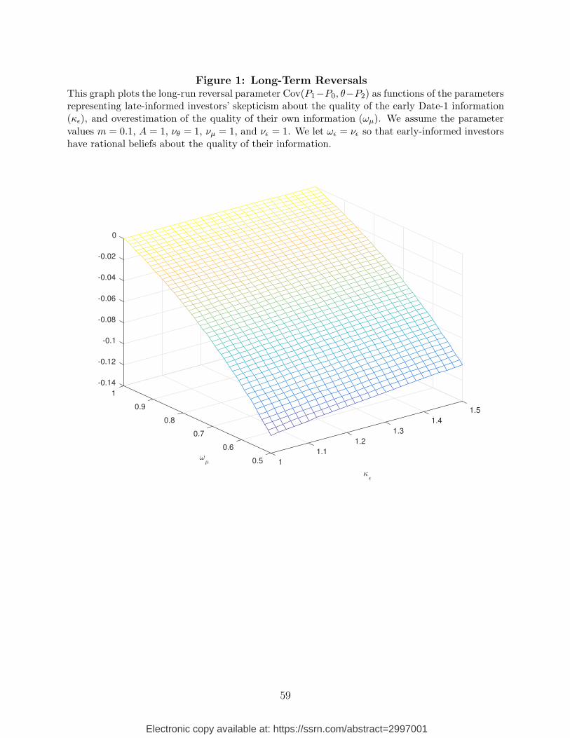
Figure 1: Long-Term ReversalsThis graph plots the long-run reversal parameter Cov(P1−P0, θ−P2) as functions of the parametersrepresenting late-informed investors’ skepticism about the quality of the early Date-1 information(κε), and overestimation of the quality of their own information (ωµ). We assume the parameter

values m = 0.1, A = 1, νθ = 1, νµ = 1, and νε = 1. We let ωε = νε so that early-informed investorshave rational beliefs about the quality of their information.

-0.14

1

-0.12

-0.1

0.9

-0.08

1.5

-0.06

0.8 1.4

-0.04

ωµ

-0.02

1.3

κε

0.7

0

1.20.6

1.1

0.5 1

59


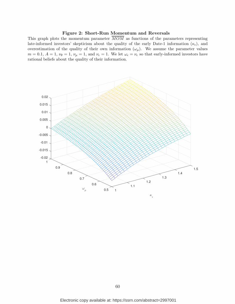
Figure 2: Short-Run Momentum and ReversalsThis graph plots the momentum parameter MOM as functions of the parameters representinglate-informed investors’ skepticism about the quality of the early Date-1 information (κε), andoverestimation of the quality of their own information (ωµ). We assume the parameter values

m = 0.1, A = 1, νθ = 1, νµ = 1, and νε = 1. We let ωε = νε so that early-informed investors haverational beliefs about the quality of their information.

-0.02

1

-0.015

-0.01

-0.005

0.91.5

0

0.005

0.8 1.4

0.01

ωµ

0.015

1.3

κε

0.7

0.02

1.20.6

1.1

0.5 1

60


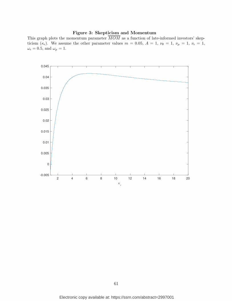
Figure 3: Skepticism and MomentumThis graph plots the momentum parameter MOM as a function of late-informed investors’ skep-ticism (κε). We assume the other parameter values m = 0.05, A = 1, νθ = 1, νµ = 1, νε = 1,ωε = 0.5, and ωµ = 1.

2 4 6 8 10 12 14 16 18 20

κε

-0.005

0

0.005

0.01

0.015

0.02

0.025

0.03

0.035

0.04

0.045

61


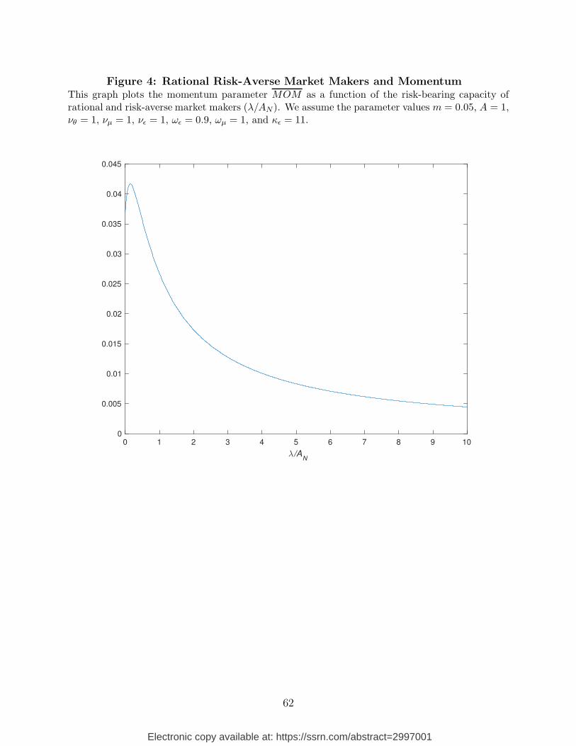
Figure 4: Rational Risk-Averse Market Makers and MomentumThis graph plots the momentum parameter MOM as a function of the risk-bearing capacity ofrational and risk-averse market makers (λ/AN). We assume the parameter values m = 0.05, A = 1,νθ = 1, νµ = 1, νε = 1, ωε = 0.9, ωµ = 1, and κε = 11.

0 1 2 3 4 5 6 7 8 9 10

λ/AN

0

0.005

0.01

0.015

0.02

0.025

0.03

0.035

0.04

0.045

62


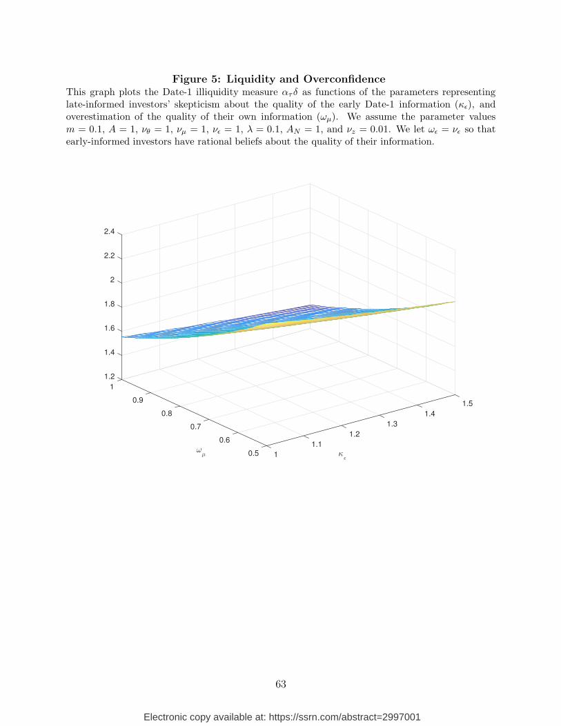
Figure 5: Liquidity and OverconfidenceThis graph plots the Date-1 illiquidity measure ατ δ as functions of the parameters representinglate-informed investors’ skepticism about the quality of the early Date-1 information (κε), andoverestimation of the quality of their own information (ωµ). We assume the parameter values

m = 0.1, A = 1, νθ = 1, νµ = 1, νε = 1, λ = 0.1, AN = 1, and νz = 0.01. We let ωε = νε so thatearly-informed investors have rational beliefs about the quality of their information.

1.2

1

1.4

1.6

0.91.5

1.8

0.8

2

1.4

ωµ

2.2

1.3

κε

0.7

2.4

1.20.6

1.1

0.5 1

63


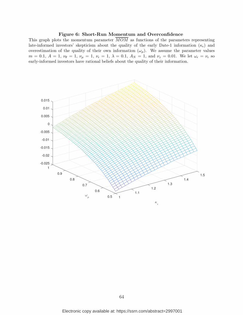
Figure 6: Short-Run Momentum and OverconfidenceThis graph plots the momentum parameter MOM as functions of the parameters representinglate-informed investors’ skepticism about the quality of the early Date-1 information (κε) andoverestimation of the quality of their own information (ωµ). We assume the parameter values

m = 0.1, A = 1, νθ = 1, νµ = 1, νε = 1, λ = 0.1, AN = 1, and νz = 0.01. We let ωε = νε soearly-informed investors have rational beliefs about the quality of their information.

-0.025

1

-0.02

-0.015

-0.01

0.91.5

-0.005

0

0.8 1.4

0.005

ωµ

0.01

1.3

κε

0.7

0.015

1.20.6

1.1

0.5 1

64


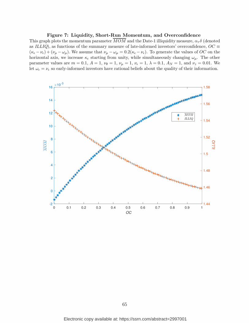
Figure 7: Liquidity, Short-Run Momentum, and OverconfidenceThis graph plots the momentum parameter MOM and the Date-1 illiquidity measure, ατ δ (denotedas ILLIQ), as functions of the summary measure of late-informed investors’ overconfidence, OC ≡(κε − νε)+ (νµ − ωµ). We assume that νµ − ωµ = 0.2(κε − νε). To generate the values of OC on the

horizontal axis, we increase κε starting from unity, while simultaneously changing ωµ. The otherparameter values are m = 0.1, A = 1, νθ = 1, νµ = 1, νε = 1, λ = 0.1, AN = 1, and νz = 0.01. We

let ωε = νε so early-informed investors have rational beliefs about the quality of their information.

0 0.1 0.2 0.3 0.4 0.5 0.6 0.7 0.8 0.9 1

OC

-2

0

2

4

6

8

10

12

14

16

MOM

×10-3

1.44

1.46

1.48

1.5

1.52

1.54

1.56

1.58

IL

LIQ

MOM

ILLIQ

65


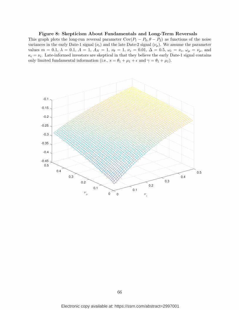
Figure 8: Skepticism About Fundamentals and Long-Term ReversalsThis graph plots the long-run reversal parameter Cov(P1 − P0, θ − P2) as functions of the noisevariances in the early Date-1 signal (νε) and the late Date-2 signal (νµ). We assume the parametervalues m = 0.1, λ = 0.1, A = 1, AN = 1, νθ = 1, νz = 0.01, ∆ = 0.5, ωε = νε, ωµ = νµ, and

κε = νε. Late-informed investors are skeptical in that they believe the early Date-1 signal containsonly limited fundamental information (i.e., s = θ1 + µ1 + ε and γ = θ1 + µ1).

-0.45

0.5

-0.4

-0.35

0.4

-0.3

0.5

-0.25

0.3 0.4

-0.2

νµ

-0.15

0.3

νε

0.2

-0.1

0.20.1

0.1

0 0

66


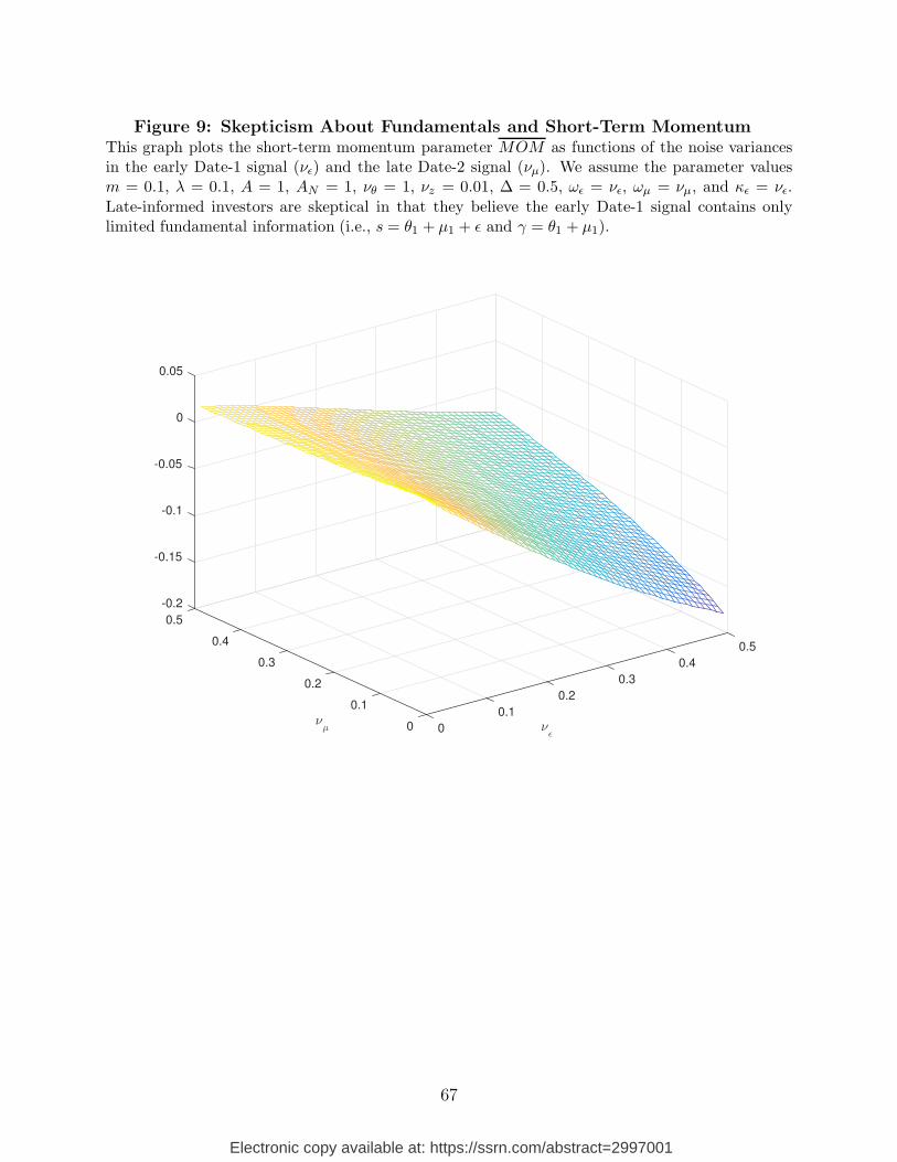
Figure 9: Skepticism About Fundamentals and Short-Term MomentumThis graph plots the short-term momentum parameter MOM as functions of the noise variancesin the early Date-1 signal (νε) and the late Date-2 signal (νµ). We assume the parameter valuesm = 0.1, λ = 0.1, A = 1, AN = 1, νθ = 1, νz = 0.01, ∆ = 0.5, ωε = νε, ωµ = νµ, and κε = νε.

Late-informed investors are skeptical in that they believe the early Date-1 signal contains onlylimited fundamental information (i.e., s = θ1 + µ1 + ε and γ = θ1 + µ1).

-0.2

0.5

-0.15

0.4

-0.1

0.5

-0.05

0.3 0.4

νµ

0

0.3

νε

0.2

0.05

0.20.1

0.1

0 0

67


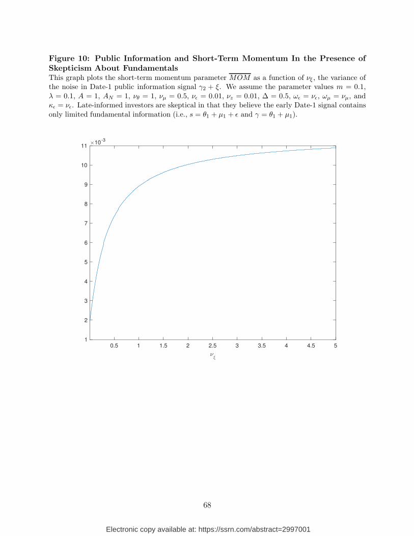
Figure 10: Public Information and Short-Term Momentum In the Presence ofSkepticism About FundamentalsThis graph plots the short-term momentum parameter MOM as a function of νξ , the variance ofthe noise in Date-1 public information signal γ2 + ξ. We assume the parameter values m = 0.1,

λ = 0.1, A = 1, AN = 1, νθ = 1, νµ = 0.5, νε = 0.01, νz = 0.01, ∆ = 0.5, ωε = νε, ωµ = νµ, andκε = νε. Late-informed investors are skeptical in that they believe the early Date-1 signal contains

only limited fundamental information (i.e., s = θ1 + µ1 + ε and γ = θ1 + µ1).

0.5 1 1.5 2 2.5 3 3.5 4 4.5 5

νξ

1

2

3

4

5

6

7

8

9

10

11×10

-3

68


Internet Appendix for

A Parsmonious Model of Momentum and Reversals in Financial Markets


In this internet appendix, we extend the setting of the main paper as follows. Like in Section 5

of the main paper, both early- and late-informed investors overestimate the quality of their

own information (indicated by the parameters ωε and ωµ), but are skeptical about the quality

of others’ information (indicated by κε). Late-informed investors are also skeptical about

the fundamental information structure; that is, from their stand point, γ = θ1 + µ1, and

s = θ1 + µ1 + ε. The scale of this skepticism is indicated by the parameter ∆. A public

information signal, t = θ + ξ, arrives either at Date 1 or Date 2. Early- and late-informed

investors are skeptical about the quality of t about θ in that they believe that the variance of

ξ equals κνξ where κ ≥ 1. There is still a mass λ of rational uninformed investors who serve

as market makers. We further assume that both the Date-1 and Date-2 supplies of the risky

security are random and are indicated by the normal random variables, z1 and z2, which are

independent and have the same variance νz. We show in Section A.3 of this appendix that

if the public information signal arrives at Date 2, the equilibrium prices take the following

forms:

P1 = Bτ1 (A.1)

and

P2 = C(τ2 + aγ2 + bs) + Dτ1 + Gt, (A.2)

where τ1 ≡ s − δ1z1 and τ2 ≡ γ − δ2z2, and B, δ1, C , δ2, a, b, D, and G are constants

to be determined, with P0 = 0. If the public information signal arrives at Date 1, we can

use a similar analysis to show that equilibrium prices take similar forms except that P1 also

depends linearly on the public signal t.

1


A.1 Momentum, Reversals, and Public Information

Note that θ, τ2, γ2, t, s, and τ1 follow a multi-variate normal distribution with mean zero

and variance-covariance matrix

νθ νθ ∆νθ νθ νθ νθ

νθ νγ + δ2

2νz ∆νγ νθ νγ νγ

∆νθ ∆νγ ∆νγ ∆νθ ∆νγ ∆νγ

νθ νθ ∆νθ νθ + νξ νθ νθ

νθ νγ ∆νγ νθ νs νs

νθ νγ ∆νγ νθ νs νs + δ2

1νz

.

We can use Eqs. (A.1) and (A.2) to compute the long-run reversal parameter,

Cov(P1 − P0, θ − P2),

and the short-run momentum parameter,

MOM = [Cov(P1 − P0, P2 − P1) + Cov(P2 − P1, θ − P2)] /2.

Intuitively, if the public signal is not very precise, then stock price patterns we demon-

strated in Section 5 still prevail. We verify this intuition using the following example. Sup-

pose that the public signal arrives at Date 2. Figures A.1 and A.2 plot the long-run reversal

parameter, Cov(P1 −P0, θ−P2), and the short-term momentum parameter, MOM as func-

tions of the signal noise variances in the Date-1 signal (νε) and Date-2 signal (νµ). The

other parameter values are in the captions of the figures. Particularly, we assume that the

public signal is sufficiently noisy (i.e., νξ = 10), and late- and early-informed investors are

sufficiently skeptical about the quality of the public signal (i.e., κ = 2). This implies that

investors put little weight on the public signal when choosing their portfolio. Consequently,

the stock price patterns here are almost identical to Figures 8 and 9 when there is no public

signal.

If the public signal is very precise, the proposition below replicates Proposition 5 of the

main paper.

Proposition A.1 (i) Suppose that the public signal arrives at Date 2. If the signal is

very precise, then long-run reversals go to zero but short-run momentum still prevails.

2


(ii) If the public signal arrives at Date 1, then, as the precision of the signal increases, both

long-run reversals and short-run momentum go to zero.

We can also use Eqs. (A.1) and (A.2) to compute the post-public-announcement drift

parameter

Cov(θ − P2, t).

Because we no longer have the closed-form solution for P2 and this drift parameter, we

use numerical analysis. Continue to suppose that the public signal arrives at Date 2 (the

analysis for the case when the public signal arrives at Date 1 is analogous). Figure A.3 plots

Cov(θ − P2, t) as functions of the skepticism about public information quality (κ), and the

late informed’s skepticism about fundamentals (∆). Other parameters are presented in the

caption of the figure. There are three notable observations. First, Cov(θ − P2, t) is positive

if ∆ is sufficiently small. This is consistent with Proposition 6 in the main paper in which

∆ = 0. Second, Cov(θ − P2, t) increases in κ. Intuitively, as the informed traders are more

skeptical about the quality of the public information (high κ), the price P2 underreacts more

to the public information, which is then followed by a greater drift. Third, as ∆ increases,

Cov(θ − P2, t) decreases and can become negative. The reason is that as the late informed

becomes more skeptical about the fundamental of the information s and γ (high ∆), at Date

2 they underreact more to the information γ. This implies that they tend to overweight and

overreact to the public information t. Therefore, the drift, Cov(θ − P2, t), is mitigated and

eventually becomes negative.

A.2 Liquidity and the Late-Informed

In this internet appendix, the supplies of the risky security at both Dates 1 and 2, z1 and z2,

are random. From Eqs. (A.1) and (A.2), z1 affects the prices at both dates, P1 and P2, and

z2 affects only P2. Thus, we compute illiquidity as the total price impact due to z1 and z2:

ILLIQ ≡ −

[

d(P1 + P2)

dz1

+dP2

dz2

]

= (B + D)δ1 + Cδ2.

Figure A.4 plots ILLIQ as functions of the parameters representing late-informed investors’

skepticism about the quality of the early Date-1 information (κε), and overestimation of the

3


quality of their own information (ωµ). Other parameters are presented in the caption of the

figure. Consistent with Figure 5 of the main paper, as late-informed become more skeptical

(i.e., as κε increases), liquidity is higher (i.e., ILLIQ decreases). As late-informed investors

overestimate the quality of their late information γ to a lesser extent (i.e., as ωµ increases),

liquidity is higher (i.e., ILLIQ decreases).

Figure A.5 verifies the main result of Figure 6 of the main paper: the momentum pa-

rameter, MOM , increases as late informed investors underestimate the quality of early

information s to a greater extent (i.e., as κε increases), and as they overestimate the quality

of their late information γ to a lesser extent (i.e., as ωµ increases).

Figure A.6 plots the momentum parameter, MOM , and the illiquidity measure, ILLIQ,

as functions of a summary measure of late-informed investors’ overconfidence, OC ≡ (κε −

νε) + (νµ − ωµ). Like in Figure 7 of the main paper, we assume that νµ − ωµ = 0.2(κε − νε)

and vary κε while simultaneously changing ωµ. Other parameter values are presented in the

caption of the figure. Consistent with Figure 7, increasing overconfidence promotes both

momentum and liquidity.

Finally, we verify in the proposition below that like in Proposition 7 of the main paper,

noise trades can reverse the short-run momentum effect.

Proposition A.2 If noise trades are sufficiently volatile (i.e., νz → ∞), then we obtain

short-run reversals, i.e., MOM → −∞.

4


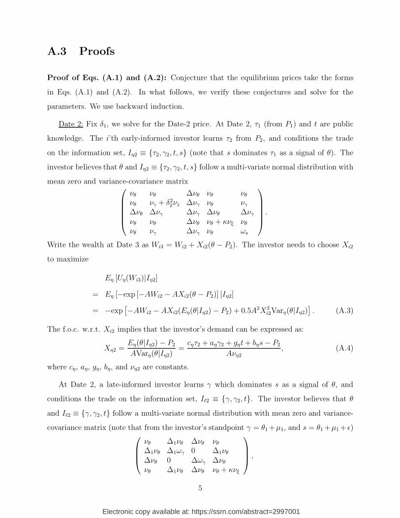
A.3 Proofs

Proof of Eqs. (A.1) and (A.2): Conjecture that the equilibrium prices take the forms

in Eqs. (A.1) and (A.2). In what follows, we verify these conjectures and solve for the

parameters. We use backward induction.

Date 2: Fix δ1, we solve for the Date-2 price. At Date 2, τ1 (from P1) and t are public

knowledge. The i’th early-informed investor learns τ2 from P2, and conditions the trade

on the information set, Iη2 ≡ {τ2, γ2, t, s} (note that s dominates τ1 as a signal of θ). The

investor believes that θ and Iη2 ≡ {τ2, γ2, t, s} follow a multi-variate normal distribution with

mean zero and variance-covariance matrix

νθ νθ ∆νθ νθ νθ

νθ νγ + δ2

2νz ∆νγ νθ νγ

∆νθ ∆νγ ∆νγ ∆νθ ∆νγ

νθ νθ ∆νθ νθ + κνξ νθ

νθ νγ ∆νγ νθ ωs

.

Write the wealth at Date 3 as Wi3 = Wi2 + Xi2(θ − P2). The investor needs to choose Xi2

to maximize

Eη [Uη(Wi3)|Iη2]

= Eη [−exp [−AWi2 − AXi2(θ − P2)] |Iη2]

= −exp[

−AWi2 − AXi2(Eη(θ|Iη2) − P2) + 0.5A2X2

i2Varη(θ|Iη2)]

. (A.3)

The f.o.c. w.r.t. Xi2 implies that the investor’s demand can be expressed as:

Xη2 =Eη(θ|Iη2) − P2

AVarη(θ|Iη2)=

cητ2 + aηγ2 + gηt + bηs − P2

Aνη2

, (A.4)

where cη, aη, gη, bη, and νη2 are constants.

At Date 2, a late-informed investor learns γ which dominates s as a signal of θ, and

conditions the trade on the information set, I`2 ≡ {γ, γ2, t}. The investor believes that θ

and I`2 ≡ {γ, γ2, t} follow a multi-variate normal distribution with mean zero and variance-

covariance matrix (note that from the investor’s standpoint γ = θ1 +µ1, and s = θ1 +µ1 + ε)

νθ ∆1νθ ∆νθ νθ

∆1νθ ∆1ωγ 0 ∆1νθ

∆νθ 0 ∆ωγ ∆νθ

νθ ∆1νθ ∆νθ νθ + κνξ

,

5


with ∆1 ≡ 1 − ∆. From a similar analysis as above, the optimal demand can be expressed

as:

X`2 =E`(θ|I`2) − P2

AVar`(θ|I`2)=

c`γ + a`γ2 + g`t − P2

Aν`2

,

where c`, a`, g`, and ν`2 are constants.

At Date 2, an uninformed rational investor learns τ1 from P1 and τ2 + aγ2 + bs from P2,

and conditions the trade on the information set, IN2 ≡ {τ2 + aγ2 + bs, t, τ1}. The investor

believes that θ and IN2 ≡ {τ2 + aγ2 + bs, t, τ1} follows a multi-variate normal distribution

with mean zero and variance-covariance matrix

νθ (1 + a∆ + b)νθ νθ νθ

(1 + a∆ + b)νθ (1 + b)2νγ + a2∆νγ (1 + a∆ + b)νθ νγ + a∆νγ + bνs

+2(1 + b)a∆νγ + δ2

2νz + b2νε

νθ (1 + a∆ + b)νθ νθ + νξ νθ

νθ νγ + a∆νγ + bνs νθ νs + δ2

1νz

.

The investor’s optimal demand can be expressed as:

XN2 =E(θ|IN2) − P2

ANVar(θ|IN2)=

cN(τ2 + aγ2 + bs) + gNt + dNτ1 − P2

ANνN2

where cN , gN , dN , and νN2 are constants.

The market clearing condition, z2 = mXη2 + (1 − m)X`2 + λXN2, implies that P2 takes

the form in Eq. (A.2). Particularly, the parameters

δ2 =Aν`2

(1 − m)c`

,

a =mν−1

η2aη + (1 − m)ν−1

`2 a`

mν−1

η2cη + (1 − m)ν−1

`2 c`

,

b =mν−1

η2bη

mν−1

η2cη + (1 − m)ν−1

`2 c`

,

C =mν−1

η2cη + (1 − m)ν−1

`2 c` + (λA−1

N A)ν−1

N2cN

mν−1

η2+ (1 − m)ν−1

`2 + (λA−1

N A)ν−1

N2

,

D =(λA−1

N A)ν−1

N2dN

mν−1

η2+ (1 − m)ν−1

`2 + (λA−1

N A)ν−1

N2

, and

G =mν−1

η2gη + (1 −m)ν−1

`2 g` + (λA−1

N A)ν−1

N2gN

mν−1

η2+ (1 − m)ν−1

`2 + (λA−1

N A)ν−1

N2

.

6


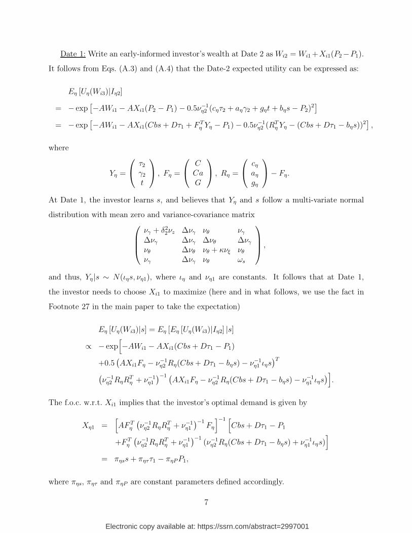
Date 1: Write an early-informed investor’s wealth at Date 2 as Wi2 = Wi1 +Xi1(P2−P1).

It follows from Eqs. (A.3) and (A.4) that the Date-2 expected utility can be expressed as:

Eη [Uη(Wi3)|Iη2]

= − exp[

−AWi1 − AXi1(P2 − P1) − 0.5ν−1

η2(cητ2 + aηγ2 + gηt + bηs − P2)

2]

= − exp[

−AWi1 − AXi1(Cbs + Dτ1 + F Tη Yη − P1) − 0.5ν−1

η2(RT

η Yη − (Cbs + Dτ1 − bηs))2]

,

where

Yη =

τ2

γ2

t

, Fη =

CCaG

, Rη =

cη

aη

gη

− Fη.

At Date 1, the investor learns s, and believes that Yη and s follow a multi-variate normal

distribution with mean zero and variance-covariance matrix

νγ + δ2

2νz ∆νγ νθ νγ

∆νγ ∆νγ ∆νθ ∆νγ

νθ ∆νθ νθ + κνξ νθ

νγ ∆νγ νθ ωs

,

and thus, Yη |s ∼ N(ιηs, νη1), where ιη and νη1 are constants. It follows that at Date 1,

the investor needs to choose Xi1 to maximize (here and in what follows, we use the fact in

Footnote 27 in the main paper to take the expectation)

Eη [Uη(Wi3)|s] = Eη [Eη [Uη(Wi3)|Iη2] |s]

∝ − exp[

−AWi1 − AXi1(Cbs + Dτ1 − P1)

+0.5(

AXi1Fη − ν−1

η2Rη(Cbs + Dτ1 − bηs) − ν−1

η1ιηs

)T

(

ν−1

η2RηR

Tη + ν−1

η1

)

−1 (

AXi1Fη − ν−1

η2Rη(Cbs + Dτ1 − bηs) − ν−1

η1ιηs

)

]

.

The f.o.c. w.r.t. Xi1 implies that the investor’s optimal demand is given by

Xη1 =[

AF Tη

(

ν−1

η2RηR

Tη + ν−1

η1

)

−1

Fη

]

−1 [

Cbs + Dτ1 − P1

+F Tη

(

ν−1

η2RηR

Tη + ν−1

η1

)

−1

(ν−1

η2Rη(Cbs + Dτ1 − bηs) + ν−1

η1ιηs)

]

= πηss + πηττ1 − πηPP1,

where πηs, πητ and πηP are constant parameters defined accordingly.

7


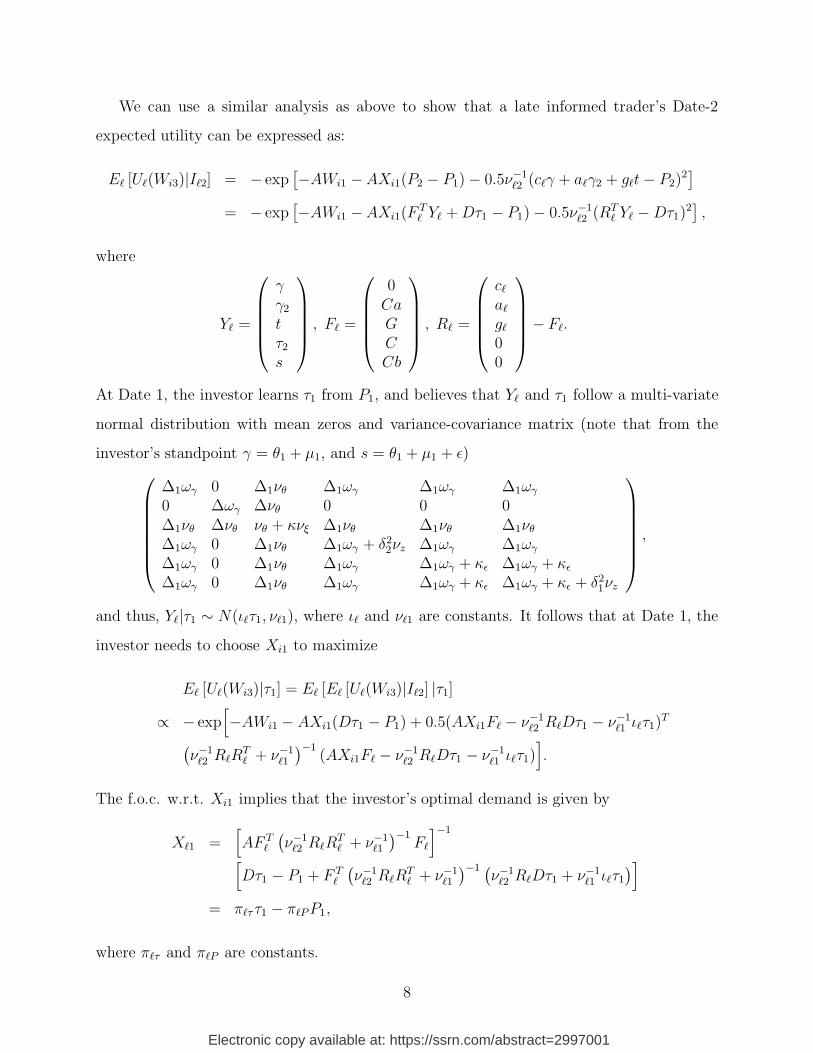
We can use a similar analysis as above to show that a late informed trader’s Date-2

expected utility can be expressed as:

E` [U`(Wi3)|I`2] = − exp[

−AWi1 −AXi1(P2 − P1) − 0.5ν−1

`2 (c`γ + a`γ2 + g`t − P2)2]

= − exp[

−AWi1 −AXi1(FT` Y` + Dτ1 − P1) − 0.5ν−1

`2 (RT` Y` − Dτ1)

2]

,

where

Y` =

γγ2

tτ2

s

, F` =

0CaGCCb

, R` =

c`

a`

g`

00

− F`.

At Date 1, the investor learns τ1 from P1, and believes that Y` and τ1 follow a multi-variate

normal distribution with mean zeros and variance-covariance matrix (note that from the

investor’s standpoint γ = θ1 + µ1, and s = θ1 + µ1 + ε)

∆1ωγ 0 ∆1νθ ∆1ωγ ∆1ωγ ∆1ωγ

0 ∆ωγ ∆νθ 0 0 0∆1νθ ∆νθ νθ + κνξ ∆1νθ ∆1νθ ∆1νθ

∆1ωγ 0 ∆1νθ ∆1ωγ + δ2

2νz ∆1ωγ ∆1ωγ

∆1ωγ 0 ∆1νθ ∆1ωγ ∆1ωγ + κε ∆1ωγ + κε

∆1ωγ 0 ∆1νθ ∆1ωγ ∆1ωγ + κε ∆1ωγ + κε + δ2

1νz

,

and thus, Y`|τ1 ∼ N(ι`τ1, ν`1), where ι` and ν`1 are constants. It follows that at Date 1, the

investor needs to choose Xi1 to maximize

E` [U`(Wi3)|τ1] = E` [E` [U`(Wi3)|I`2] |τ1]

∝ − exp[

−AWi1 − AXi1(Dτ1 − P1) + 0.5(AXi1F` − ν−1

`2 R`Dτ1 − ν−1

`1 ι`τ1)T

(

ν−1

`2 R`RT` + ν−1

`1

)

−1

(AXi1F` − ν−1

`2 R`Dτ1 − ν−1

`1 ι`τ1)]

.


X`1 =[

AF T`

(

ν−1

`2 R`RT` + ν−1

`1

)

−1

F`

]

−1

[

Dτ1 − P1 + F T`

(

ν−1

`2 R`RT` + ν−1

`1

)

−1 (

ν−1

`2 R`Dτ1 + ν−1

`1 ι`τ1

)

]

= π`ττ1 − π`PP1,

where π`τ and π`P are constants.

8


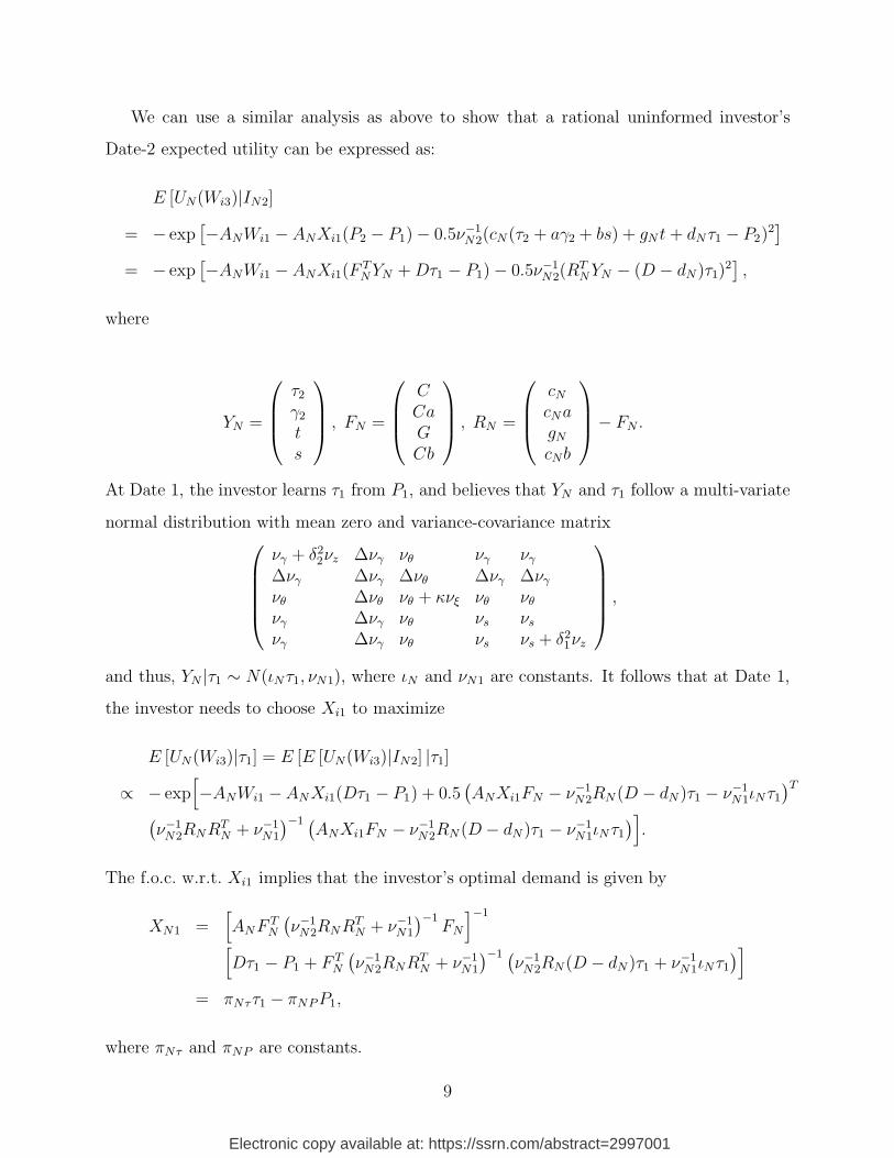
We can use a similar analysis as above to show that a rational uninformed investor’s

Date-2 expected utility can be expressed as:

E [UN(Wi3)|IN2]

= − exp[

−ANWi1 − ANXi1(P2 − P1) − 0.5ν−1

N2(cN (τ2 + aγ2 + bs) + gN t + dNτ1 − P2)

2]

= − exp[

−ANWi1 − ANXi1(FTNYN + Dτ1 − P1) − 0.5ν−1

N2(RT

NYN − (D − dN )τ1)2]

,

where

YN =

τ2

γ2

ts

, FN =

CCaGCb

, RN =

cN

cNagN

cNb

− FN .

At Date 1, the investor learns τ1 from P1, and believes that YN and τ1 follow a multi-variate

normal distribution with mean zero and variance-covariance matrix

νγ + δ2

2νz ∆νγ νθ νγ νγ

∆νγ ∆νγ ∆νθ ∆νγ ∆νγ

νθ ∆νθ νθ + κνξ νθ νθ

νγ ∆νγ νθ νs νs

νγ ∆νγ νθ νs νs + δ2

1νz

,

and thus, YN |τ1 ∼ N(ιNτ1, νN1), where ιN and νN1 are constants. It follows that at Date 1,

the investor needs to choose Xi1 to maximize

E [UN(Wi3)|τ1] = E [E [UN(Wi3)|IN2] |τ1]

∝ − exp[

−ANWi1 −ANXi1(Dτ1 − P1) + 0.5(

ANXi1FN − ν−1

N2RN (D − dN )τ1 − ν−1

N1ιNτ1

)T

(

ν−1

N2RNRT

N + ν−1

N1

)

−1 (

ANXi1FN − ν−1

N2RN (D − dN )τ1 − ν−1

N1ιNτ1

)

]

.


XN1 =[

ANF TN

(

ν−1

N2RNRT

N + ν−1

N1

)

−1

FN

]

−1

[

Dτ1 − P1 + F TN

(

ν−1

N2RNRT

N + ν−1

N1

)

−1 (

ν−1

N2RN (D − dN )τ1 + ν−1

N1ιNτ1

)

]

= πNττ1 − πNPP1,

where πNτ and πNP are constants.

9


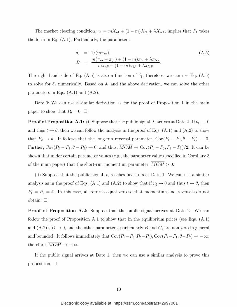
The market clearing condition, z1 = mXη1 + (1 − m)X`1 + λXN1, implies that P1 takes

the form in Eq. (A.1). Particularly, the parameters

δ1 = 1/(mπηs), (A.5)

B =m(πηs + πητ) + (1 − m)π`τ + λπNτ

mπηP + (1 − m)π`P + λπNP

.

The right hand side of Eq. (A.5) is also a function of δ1; therefore, we can use Eq. (A.5)

to solve for δ1 numerically. Based on δ1 and the above derivation, we can solve the other

parameters in Eqs. (A.1) and (A.2).

Date 0: We can use a similar derivation as for the proof of Proposition 1 in the main

paper to show that P0 = 0. �

Proof of Proposition A.1: (i) Suppose that the public signal, t, arrives at Date 2. If νξ → 0

and thus t → θ, then we can follow the analysis in the proof of Eqs. (A.1) and (A.2) to show

that P2 → θ. It follows that the long-run reversal parameter, Cov(P1 − P0, θ − P2) → 0.

Further, Cov(P2 − P1, θ − P2) → 0, and thus, MOM → Cov(P1 − P0, P2 − P1)/2. It can be

shown that under certain parameter values (e.g., the parameter values specified in Corollary 3

of the main paper) that the short-run momentum parameter, MOM > 0.

(ii) Suppose that the public signal, t, reaches investors at Date 1. We can use a similar

analysis as in the proof of Eqs. (A.1) and (A.2) to show that if νξ → 0 and thus t → θ, then

P1 = P2 = θ. In this case, all returns equal zero so that momentum and reversals do not

obtain. �

Proof of Proposition A.2: Suppose that the public signal arrives at Date 2. We can

follow the proof of Proposition A.1 to show that in the equilibrium prices (see Eqs. (A.1)

and (A.2)), D → 0, and the other parameters, particularly B and C , are non-zero in general

and bounded. It follows immediately that Cov(P1−P0, P2−P1), Cov(P2−P1, θ−P2) → −∞;

therefore, MOM → −∞.

If the public signal arrives at Date 1, then we can use a similar analysis to prove this

proposition. �

10


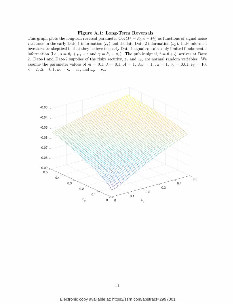
Figure A.1: Long-Term ReversalsThis graph plots the long-run reversal parameter Cov(P1 − P0, θ − P2) as functions of signal noisevariances in the early Date-1 information (νε) and the late Date-2 information (νµ). Late-informedinvestors are skeptical in that they believe the early Date-1 signal contains only limited fundamental

information (i.e., s = θ1 + µ1 + ε and γ = θ1 + µ1). The public signal, t = θ + ξ, arrives at Date2. Date-1 and Date-2 supplies of the risky security, z1 and z2, are normal random variables. We

assume the parameter values of m = 0.1, λ = 0.1, A = 1, AN = 1, νθ = 1, νz = 0.01, νξ = 10,κ = 2, ∆ = 0.1, ωε = κε = νε, and ωµ = νµ.

-0.09

0.5

-0.08

-0.07

0.40.5

-0.06

0.3

-0.05

0.4

νµ

-0.04

0.3

νε

0.2

-0.03

0.20.1

0.1

0 0

11


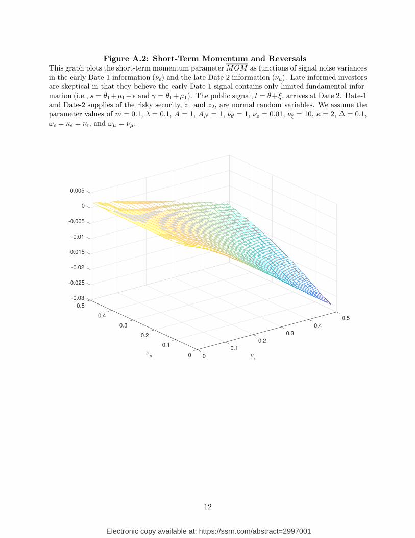
Figure A.2: Short-Term Momentum and ReversalsThis graph plots the short-term momentum parameter MOM as functions of signal noise variancesin the early Date-1 information (νε) and the late Date-2 information (νµ). Late-informed investorsare skeptical in that they believe the early Date-1 signal contains only limited fundamental infor-

mation (i.e., s = θ1 +µ1 +ε and γ = θ1 +µ1). The public signal, t = θ+ξ, arrives at Date 2. Date-1and Date-2 supplies of the risky security, z1 and z2, are normal random variables. We assume the

parameter values of m = 0.1, λ = 0.1, A = 1, AN = 1, νθ = 1, νz = 0.01, νξ = 10, κ = 2, ∆ = 0.1,ωε = κε = νε, and ωµ = νµ.

-0.03

0.5

-0.025

-0.02

0.4

-0.015

0.5

-0.01

0.3 0.4

-0.005

νµ

0

0.3

νε

0.2

0.005

0.20.1

0.1

0 0

12


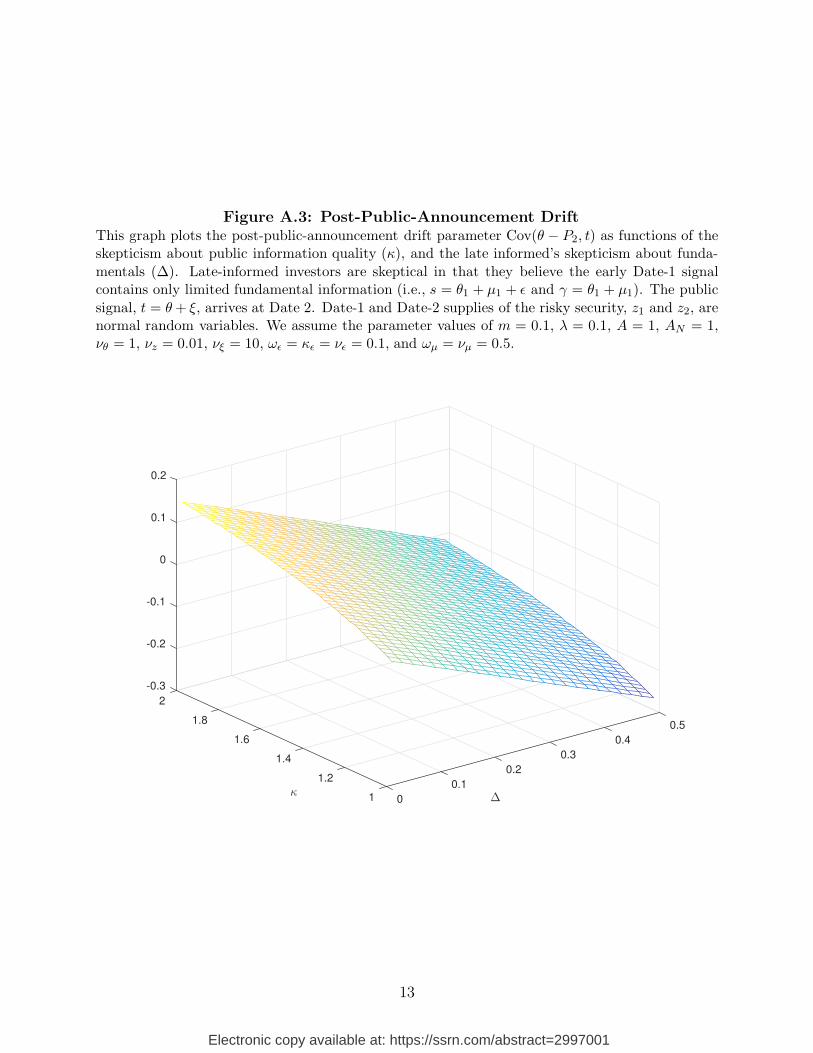
Figure A.3: Post-Public-Announcement DriftThis graph plots the post-public-announcement drift parameter Cov(θ − P2, t) as functions of theskepticism about public information quality (κ), and the late informed’s skepticism about funda-

mentals (∆). Late-informed investors are skeptical in that they believe the early Date-1 signalcontains only limited fundamental information (i.e., s = θ1 + µ1 + ε and γ = θ1 + µ1). The public

signal, t = θ + ξ, arrives at Date 2. Date-1 and Date-2 supplies of the risky security, z1 and z2, arenormal random variables. We assume the parameter values of m = 0.1, λ = 0.1, A = 1, AN = 1,νθ = 1, νz = 0.01, νξ = 10, ωε = κε = νε = 0.1, and ωµ = νµ = 0.5.

-0.3

2

-0.2

1.8

-0.1

0.5

0

1.6 0.4

κ

0.1

0.3

∆

1.4

0.2

0.21.2

0.1

1 0

13


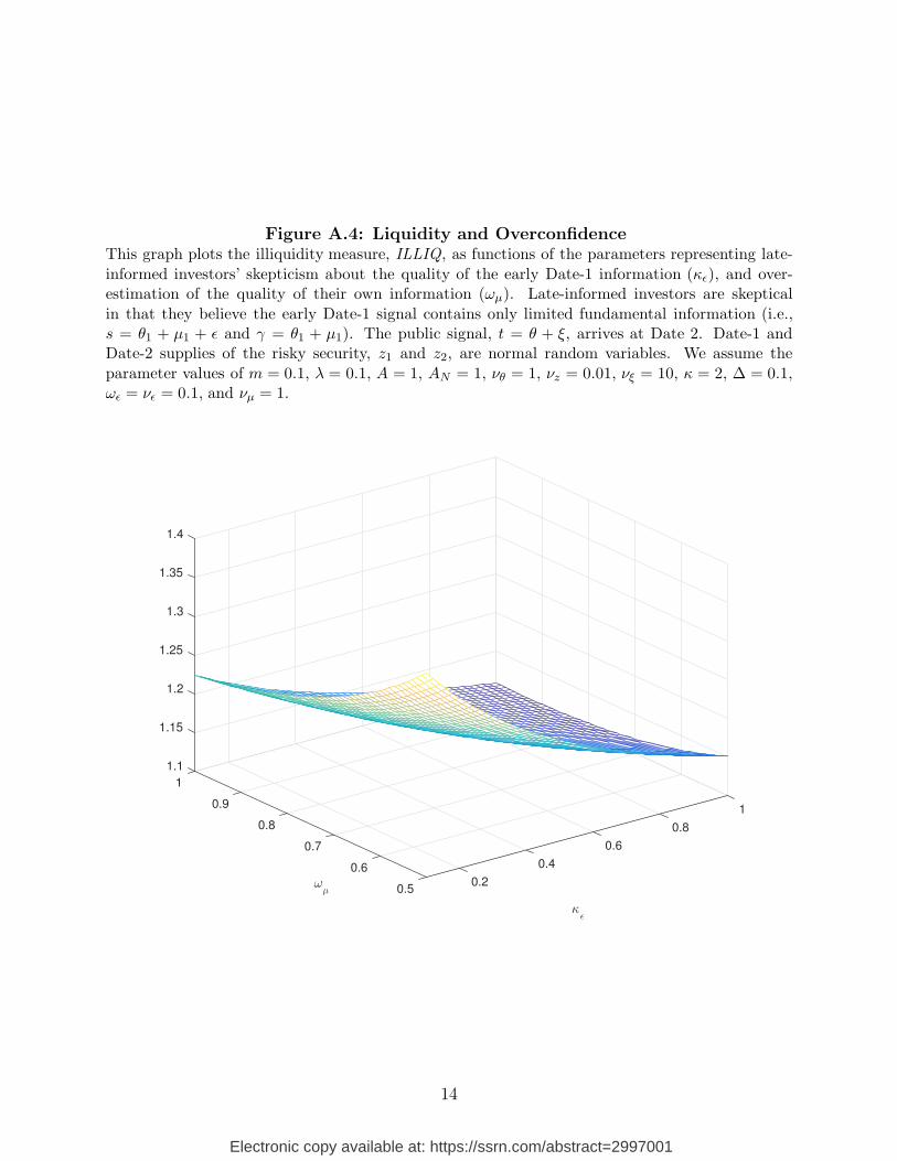
Figure A.4: Liquidity and OverconfidenceThis graph plots the illiquidity measure, ILLIQ, as functions of the parameters representing late-

informed investors’ skepticism about the quality of the early Date-1 information (κε), and over-estimation of the quality of their own information (ωµ). Late-informed investors are skeptical

in that they believe the early Date-1 signal contains only limited fundamental information (i.e.,s = θ1 + µ1 + ε and γ = θ1 + µ1). The public signal, t = θ + ξ, arrives at Date 2. Date-1 andDate-2 supplies of the risky security, z1 and z2, are normal random variables. We assume the

parameter values of m = 0.1, λ = 0.1, A = 1, AN = 1, νθ = 1, νz = 0.01, νξ = 10, κ = 2, ∆ = 0.1,ωε = νε = 0.1, and νµ = 1.

1.1

1

1.15

1.2

0.91

1.25

0.8

1.3

0.8

ωµ

1.35

κε

0.60.7

1.4

0.40.6

0.20.5

14


Figure A.5: Short-Run Momentum and OverconfidenceThis graph plots the momentum parameter MOM as functions of the parameters representinglate-informed investors’ skepticism about the quality of the early Date-1 information (κε), and

overestimation of the quality of their own information (ωµ). Late-informed investors are skepticalin that they believe the early Date-1 signal contains only limited fundamental information (i.e.,

s = θ1 + µ1 + ε and γ = θ1 + µ1). The public signal, t = θ + ξ, arrives at Date 2. Date-1 andDate-2 supplies of the risky security, z1 and z2, are normal random variables. We assume theparameter values of m = 0.1, λ = 0.1, A = 1, AN = 1, νθ = 1, νz = 0.01, νξ = 10, κ = 2, ∆ = 0.1,

ωε = νε = 0.1, and νµ = 1.

-0.01

1

-0.005

0

0.005

0.91

0.01

0.015

0.8 0.8

0.02

ωµ

0.025

κε

0.60.7

0.03

0.40.6

0.20.5

15


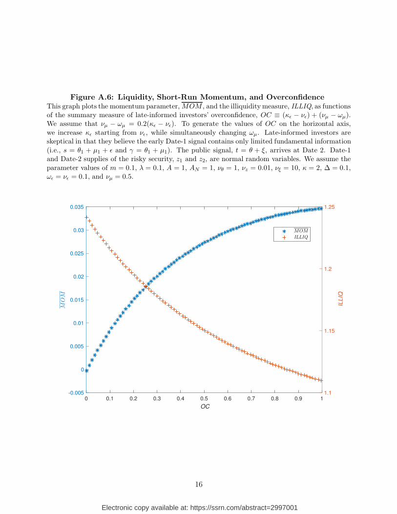
Figure A.6: Liquidity, Short-Run Momentum, and OverconfidenceThis graph plots the momentum parameter, MOM , and the illiquidity measure, ILLIQ, as functionsof the summary measure of late-informed investors’ overconfidence, OC ≡ (κε − νε) + (νµ − ωµ).We assume that νµ − ωµ = 0.2(κε − νε). To generate the values of OC on the horizontal axis,

we increase κε starting from νε, while simultaneously changing ωµ. Late-informed investors areskeptical in that they believe the early Date-1 signal contains only limited fundamental information

(i.e., s = θ1 + µ1 + ε and γ = θ1 + µ1). The public signal, t = θ + ξ, arrives at Date 2. Date-1and Date-2 supplies of the risky security, z1 and z2, are normal random variables. We assume the

parameter values of m = 0.1, λ = 0.1, A = 1, AN = 1, νθ = 1, νz = 0.01, νξ = 10, κ = 2, ∆ = 0.1,ωε = νε = 0.1, and νµ = 0.5.

0 0.1 0.2 0.3 0.4 0.5 0.6 0.7 0.8 0.9 1

OC

-0.005

0

0.005

0.01

0.015

0.02

0.025

0.03

0.035

MOM

1.1

1.15

1.2

1.25

IL

LIQ

MOM

ILLIQ

16


A Parsimonious Model of Momentum and Reversals in ...

Documents

Transcript of A Parsimonious Model of Momentum and Reversals in ...