Parsimonious reconstruction of 2D MHD equilibrium states...

Ollscoil na h-Éireann, Corcaigh

Parsimonious reconstruction of 2D MHD equilibrium

states using database training methods

A thesis submitted for the degree of

Master of Science

by

Shane O’Mahony

October 2011

Academic Supervisor: Dr. P. Mc Carthy

Head of Department: Prof. J. McInerney

Department of Physics

University College Cork

Abstract

Controlled thermonuclear fusion is introduced and the conditions for a self-sustaining

fusion reactor are obtained. Plasma confinement by magnetic fields, especially by toka-

maks, is described. The magneto-hydrodynamic equations are presented and the equation

for an axisymmetric MHD equilibrium is introduced.

Function Parameterization (FP) has been in use for identification of equilibrium pa-

rameters on the ASDEX Upgrade tokamak since 1991. FP, which has the reliability

advantage over conventional equilibrium solvers of being predictive rather than interpre-

tive, was also used to recover the equilibrium poloidal flux function by the brute force

calculation of the magnetic flux ( (R, Z)) as a scalar parameter at each point on a

spatial grid using scalar plasma parameters recovered in real time using magnetic data.

A new FP based algorithm for full equilibrium flux recovery was introduced which uses

the Singular Value Decomposition (SVD) of a training equilibrium. SVD was used to

generate eigenfaces as well as Fourier-like amplitudes that are regressed so that they can

be calculated using the real time magnetic data. These can then be used to recover the

magnetic flux.

The aim of the thesis was to investigate if the application of eigenface analysis results in

improvements in equilibrium reconstruction when used in conjunction with FP. The work

done during the project builds on that done on applying FP to equilibrium reconstruction

in [1]. Code was written in Mathematica to perform SVD, FP and to analyse results.

Contents

1 Introduction 3

1.1 Nuclear Power . . . . . . . . . . . . . . . . . . . . . . . . . . . . . . . . . 3

1.2 Nuclear Fusion . . . . . . . . . . . . . . . . . . . . . . . . . . . . . . . . . 4

1.3 Plasma . . . . . . . . . . . . . . . . . . . . . . . . . . . . . . . . . . . . . . 5

1.3.1 Generation of Plasmas . . . . . . . . . . . . . . . . . . . . . . . . . 5

1.3.2 Plasma Temperature . . . . . . . . . . . . . . . . . . . . . . . . . . 5

1.3.3 Degree of Ionization . . . . . . . . . . . . . . . . . . . . . . . . . . 6

1.3.4 The Electron Energy Distribution Function . . . . . . . . . . . . . 6

1.4 Magnetohydrodynamics . . . . . . . . . . . . . . . . . . . . . . . . . . . . 7

1.5 Magnetic Confinement . . . . . . . . . . . . . . . . . . . . . . . . . . . . . 10

1.6 ASDEX Upgrade . . . . . . . . . . . . . . . . . . . . . . . . . . . . . . . . 14

1.6.1 The control algorithm . . . . . . . . . . . . . . . . . . . . . . . . . 18

1.7 Equilibrium reconstruction . . . . . . . . . . . . . . . . . . . . . . . . . . 21

1.8 Outline of the Thesis . . . . . . . . . . . . . . . . . . . . . . . . . . . . . . 22

2 Background Theory 23

2.1 A review of basic statistics . . . . . . . . . . . . . . . . . . . . . . . . . . . 23

2.2 Singular Value Decomposition . . . . . . . . . . . . . . . . . . . . . . . . . 24

2.3 Eigenfaces . . . . . . . . . . . . . . . . . . . . . . . . . . . . . . . . . . . . 26

2.4 Principal Component Analysis . . . . . . . . . . . . . . . . . . . . . . . . 27

2.5 Multiple Linear Regression . . . . . . . . . . . . . . . . . . . . . . . . . . 28

2.6 Function Parameterization . . . . . . . . . . . . . . . . . . . . . . . . . . . 29

2.6.1 Basic Concepts . . . . . . . . . . . . . . . . . . . . . . . . . . . . . 29

2.6.2 The data base . . . . . . . . . . . . . . . . . . . . . . . . . . . . . 29

2.6.3 Dimension reduction . . . . . . . . . . . . . . . . . . . . . . . . . . 30

2.6.4 Use of incremental signal to noise ratio as selection criterion for the

Principal Components . . . . . . . . . . . . . . . . . . . . . . . . . 31

2.6.5 Optimal suppression of signal noise by using filtering techniques . 31

2.7 Error analysis . . . . . . . . . . . . . . . . . . . . . . . . . . . . . . . . . . 34

2.7.1 The percentage error . . . . . . . . . . . . . . . . . . . . . . . . . . 34

2.7.2 An alternative method of calculating the percentage error . . . . . 34

1

3 Reconstruction of 2D MHD equilibrium states using database training

methods 38

3.1 The training database . . . . . . . . . . . . . . . . . . . . . . . . . . . . . 38

3.2 Singular Value Decomposition of the training database . . . . . . . . . . . 42

3.2.1 SVD of the magnetic flux . . . . . . . . . . . . . . . . . . . . . . . 42

3.2.2 SVD of the current profile . . . . . . . . . . . . . . . . . . . . . . . 46

3.3 Principal component analysis of magnetic measurements . . . . . . . . . . 50

3.4 Recovering the Fourier moments using Function Parameterization . . . . . 52

3.5 E↵ectiveness of noise suppression . . . . . . . . . . . . . . . . . . . . . . . 56

3.6 Eigenface reconstruction . . . . . . . . . . . . . . . . . . . . . . . . . . . . 57

4 Conclusion 63

A Table of notations 64

B References 65

C Mathematica Code 67

2

Chapter 1

Introduction

1.1 Nuclear Power

This Section is based on [1, Section 1.1] and [2]

The prediction of the exhaustion of fossil fuel reserves and the growth in demand for

electrical power (mostly by developing countries such as China and India) were powerful

stimulants in spurring the development of nuclear power for peaceful purposes in the

aftermath of the Second World War. The appeal of nuclear power can be seen from a

graph of packing fraction versus nuclear mass (Fig. 1). The packing fraction is defined

as P = M�A

A

where M is the actual mass in amu and A is the nuclear mass number.

amu is defined as one twelfth of the rest mass of an unbound neutral atom of carbon-12

in its nuclear and electronic ground state and has a value of 1.660538921⇥1027 kg. In

general, a lower packing fraction indicates a greater binding energy per nucleon and hence

a greater stability. Atoms with a lower binding energy are easier to “break apart” and

release energy from. Both the splitting of heavy nuclei and the fusing of light nuclei

results in a net release of energy according to Einstein’s mass-energy equivalence relation

(E = (�m)c2) where �m is the net loss of rest mass of the reaction products (due to the

loss of binding energy) and c is the speed of light (c =299,792,458 m/s ).

Nuclear fission is a nuclear reaction in which the nucleus of an atom splits into two

or more lighter nuclei, producing neutrons and a net release of energy. These neutrons

can in turn split more heavy nuclei, leading to a very rapid release of energy which must

be controlled by the introduction of non-fissile neutron-absorbing material (such as heavy

water (HDO) or graphite) into the reactive mass. The kinetic energy of the reaction

products is utilized to produce steam which then drives electricity generating turbines.

Fission power is used on a large scale in countries such as France, the UK and the US.

Fusion energy is generated when two light nuclei fuse to form a heavier nucleus (and at

least one other nucleon to satisfy energy and momentum conservation) where the rest mass

of the reactants exceeds that of the products. A key di↵erence between fusion and fission

is the fact that in order to fuse, two nuclei must overcome their mutual electrostatic

repulsion by approaching each other su�ciently closely that the short range attractive

3

Figure 1.1: Packing fractions

strong nuclear force allows the two nuclei to fuse. Nuclear fusion is what powers stars

and is currently the subject of worldwide research for the generation of electricity.

1.2 Nuclear Fusion


The most promising nuclear reaction to be used for fusion is

21D+3

1 T !42 He(3.5 MeV) +1

0 n(14.1 MeV). (1.1)

Deuterium occurs naturally as heavy water (HDO), with an abundance of nDnH

= 1.5⇥10�4. Tritium does not occur naturally but the neutrons released in the above reaction

can be used to produce tritium from lithium:

10n +6

3 Li !42 He(2.1 MeV) +3

1 T (2.7 MeV). (1.2)

Since ions are positively charged, the Coulomb force of repulsion has to be overcome

before the reactions can occur. Therefore, the nuclei have to be accelerated to very high

kinetic energies in order to penetrate the Coulomb barrier. A beam of deuterons from an

accelerator cannot be used as it can be shown that if the beam is directed at a target of

solid tritium, most of the energy is lost in ionizing and heating the target and in elastic

collisions. The solution is to form a Maxwellian plasma of deuterium and tritium in which

the fast particles undergo fusion. A plasma is Maxwellian if the probability distribution

function of the plasma’s energy is described by Maxwell-Boltzmann statistics, i.e. the

expected number of particles (Ni

) with energy ✏i

is given by

Ni

=N

Zgi

e�✏i/kT , (1.3)

4

where gi

is the degeneracy of energy level i, k is Boltzmann’s constant, T is the ab-

solute temperature and N is the total number of particles. Elastic collisions do not

change the distribution function if it is Maxwellian and, apart from bremsstrahlung losses

(bremsstrahlung is electromagnetic radiation produced by the deceleration of a charged

particle when deflected by another charged particle), the energy used to heat the plasma

is retained until the particles react or escape from the chamber.

1.3 Plasma

This Section is based on [2 - 5]

A plasma, often referred to as the fourth state of matter, is a gas which contains

ionized particles. The presence of these ionized particles make the plasma electrically

conductive so that it responds strongly to electromagnetic fields. Common examples of

plasmas are stars and neon signs. Some ranges of plasma parameters are shown in table

1.1.

Size (m) 10�6 (for lab plasmas)102 (Lightning)

Density (particle/m3 ) 107

1032 (Inertial confinement plasmas)Temperature (K) 107 (Solar core)

108 (Magnetic fusion plasma)Magnetic Fields (T) 10�4 (Lab plasma)

1011 (Near a neutron star)

Table 1.1: Some properties of plasmas

1.3.1 Generation of Plasmas

Creation of a plasma requires partial ionization of the neutral atoms/ molecules of a

medium. There are several ways to cause ionization: collisions of energetic particles,

strong electric fields acting on bond electrons, or ionizing radiation. The kinetic energy

for ionizing collisions may come from the heat of chemical or nuclear reactions of the

medium (for example, flames). Alternatively, already released charged particles may be

accelerated by electric fields, generated electromagnetically or by radiation fields.

1.3.2 Plasma Temperature

Plasma temperature (measured in Kelvin or electronvolts) can be described as a measure

of the thermal kinetic energy per particle. Very high temperatures (on the order of millions

of Kelvin) are usually needed to sustain the ionization of the plasma. The degree of plasma

ionization is determined by the electron temperature and the ionization energy. If the

probability function of the electron velocity in the plasma follows a Maxwell-Boltzmann

distribution (see Section 1.2), then the electron temperature is the temperature of the

5

distribution. If the electrons do not follow a Maxwell-Boltzmann distribution, then it is

still possible to define an e↵ective temperature equal to two-thirds of the average electron

energy.

1.3.3 Degree of Ionization

For a plasma to exist, ionization is necessary. The term “plasma density” by itself usually

refers to the “electron density”, that is, the number of free electrons per unit volume.

The degree of ionization of a plasma is the proportion of atoms that have lost (or gained)

electrons. Even a partially ionized gas in which as little as 1% of the particles are ionized

can be considered a plasma. The degree of ionization, ↵, is defined as:

↵ =ni

(ni

+ na

), (1.4)

where ni

is the number density of ions and na

is the number density of neutral atoms.

The electron density is related to this by the average charge state < Z > of the ions

through

ne

=< Z > ni

, (1.5)

where ne

is the number density of the electrons.

1.3.4 The Electron Energy Distribution Function

In general, the electron energy distribution function (EEDF) is not Maxwellian for a

plasma (i.e. it does not follow a Maxwell-Boltzmann distribution). However, this is not

the case for large tokamaks (see Section 1.6) like ASDEX Upgrade. For large tokamaks,

the energy confinement time(of order 100 ms) greatly exceeds typical collision times. The

collision rate for electrons in a thermal plasma (⌫e

in Hz) is given by [27]

⌫e

=2.9⇥ 10�6 ⇥ n⇥ ln(⇤)

T 1.5(1.6)

where n is the density (in cm�3), T is the temperature in eV and ln⇤ is the Coulomb

logarithm. In general (for ASDEX Upgrade), n = 1013 cm�3, T = 1 keV and the Coulomb

logarithm is approximately 15. Thus, ⌫e

= 13750 /s which gives a collision time (⌧e

) of the

order of 100 µs or 0.001 of the confinement time. Thus the assumption of a Maxwellian

distribution is a good one.

6

1.4 Magnetohydrodynamics

This Section is based on [1, Section 1.4] and [2 ]

The simplest useful model of fusion plasmas are the magnetohydrodynamic (MHD)

equations. These are a combination of the Navier-Stokes equations of fluid dynamics and

Maxwell’s equations of electromagnetism. The equations (neglecting the displacement

current) are shown below:

@⇢

@t+r · (⇢v) = 0 (1.7)

⇢@v

@t+ ⇢(v ·r)v +rp� J⇥B = 0 (1.8)

@p

@t+ v ·rp+

5

3pr · v = 0 (1.9)

@B

@t+r⇥E = 0 (1.10)

µ0J = r⇥B (1.11)

r ·D = ⇢ (1.12)

r.B = 0 (1.13)

In these equations, ⇢ is the mass density, v is the flow velocity, p is the pressure, J

is the current density, B is the magnetic field, E is the electric field, D is the electric

displacement field and µ0 is the magnetic permeability in a vacuum. The first three

equations describe mass, momentum and energy conservation for an ideal fluid having an

adiabatic index (the ratio of heat capacity at constant pressure to the heat capacity at

constant volume) � = 5/3. The final four equations are Maxwell’s equations for an ideally

conducting medium with the displacement current set to zero. This system of equations

provide a single-fluid description of macroscopic plasma behaviour.

However, many e↵ects that are important in tokamak physics are neglected in the

MHD model. There is no heat conduction, particle di↵usion, resistivity, or viscosity in

the model. There is no displacement current or space charge, and also all particle kinetic

e↵ects are ignored. To take these into account, other mathematical models are employed

in order to represent either di↵usive processes on the longer time scale, or a variety of

waves and instabilities on short timescales.

The data studied in this thesis are those of a steady-state (slowly evolving) plasma,

where v = 0 and @/@t = 0 in the MHD equations and (from Eqn. (1.8))

J⇥B = µ�10 (r⇥B)⇥B = rp. (1.14)

In the case of axisymmetry ( @@�

= 0) in cylindrical coordinates (R,�, Z), Eqn. (1.14)

reduces to a scalar partial di↵erential equation. First, write the total magnetic field as

B = Btor

+Bpol

where Btor

= (0, B�

, 0) and Bpol

= (BR

, 0, BZ

). Since @

@�

= 0, all three

7

components are functions of R, Z only. If A is the magnetic vector potential, then writing

Bpol

= r⇥A gives

Bpol

= (�@A

�

@z,@A

R

@Z� @A

Z

@R,1

R

@(RA�

)

@R) (1.15)

The only constraint on AR

and AZ

is that the � component of Bpol

vanishes. There-

fore, AR

= AZ

= 0 and then B = r⇥(A�

�)+B�

�. Then, use Stokes’ theorem to express

A�

in terms of the poloidal flux enclosed by a magnetic surface ( pol

) and get (note: the

contour Cpol

is chosen to be a circle of radius R)

pol

=

Z

Spol

B · dS (1.16)

=

Z

Spol

(r⇥A�

�) · dS+

Z

Spol

B�

� · dS (1.17)

=

I

Cpol

A�

� · dl+ 0 (1.18)

= 2⇡RA�

. (1.19)

Defining a stream function ⌘ pol

/2⇡ gives (noting that r� = �/R)

B = r⇥ ( r�) +B�

� (1.20)

= r ⇥r�+B�

� (1.21)

= � 1

R

@

@ZR+

1

R

@

@RZ +B

�

�. (1.22)

Using Eqn. (1.22), the current density J = µ�10 r⇥B can be written as

µ0J = r⇥Bpol

+r⇥Btor

(1.23)

= (� 1

R

@2

@Z2� @

@R

1

R

@

@R)�+r⇥ (B

�

Rr�) (1.24)

= � 1

R4⇤ �+r(RB

�

)⇥r�, (1.25)

where 4⇤ is an operator defined as

4⇤ = R@

@R

1

R

@

@R+@2

@Z2. (1.26)

Substitution of equations (1.21) and (1.25) into the force balance equation rp = J⇥B

gives (noting that r(RB�

) · � = 0) due to axisymmetry

8

µ0p0( )r = (� 1

R4⇤ +r(RB

)⇥r�)⇥ (r ⇥r�+B�

�) (1.27)

= � 1

R24⇤ r �

B�

Rr(RB

�

) (1.28)

For this equation to hold everywhere, r(RB�

) must be parallel to r . Therefore, RB�

must be a surface quantity, say F(�). Since J ·rp = 0, current density field lines must

also lie on magnetic surfaces. If the poloidal current is

Ipol

=

Z

Spol

J · dS, (1.29)

then substituting for J from Eqn. (1.22) gives

µ0Ipol

=

Z

Spol

r⇥B · dS (1.30)

=

Z

Spol

� 1

R4⇤ � · dS+

Z

Spol

(r⇥ (B�

Rr�)) · dS (1.31)

= 0 +

I

Cpol

B�

� · dl (1.32)

= 2⇡RB�

. (1.33)

Therefore, RB�

⌘ F ( ) = µ0Ipol

/2⇡ is proportional to the poloidal current and rearrang-

ing Eqn. (1.28) gives

�4⇤ = µ0R2p0( ) + FF 0( ) (1.34)

where p and F are arbitary functions of and p0( ) = dp

d

and FF 0( ) = dF

2

d

. Also, Eqn.

(1.25) can be written as

µ0J = � 1

R4⇤ �+ F 0( )r ⇥r� (1.35)

= � 1

R4⇤ �� F 0

R

@

@ZR+

F 0

R

@

@RZ (1.36)

⌘ µ0(Jtor

+ Jpol

), (1.37)

which then gives

�4⇤ = µ0RJ�

(1.38)

Eqn. (1.34) is known as the Grad-Shafranov equation (GSE) and is a non-linear

elliptic partial di↵erential equation which is solved by specifying the functions p = p( )

and F = F ( ), together with boundary conditions or externally imposed constraints on

9

and then inverting 4⇤ to determine = (R,Z). For a fusion plasma, p refers to the

pressure in the plasma and F ( ) ⌘ RB�

. The boundary conditions are that be 0 at R=0

(the axis of the axisymmetric system) and = 0 at R = 1. The usual solution requires

the numerical iteration of the above process until converges to a consistent solution.

The plasma equilibrium is described by solutions of the GSE with known additional

sources (consisting of external conductor currents) for the flux function and boundary

conditions at infinity and at the axis. The plasma is contained in a bounded toroidal

region surrounded by a vacuum magnetic field in which the pressure and current density

vanish. The spatial location of the plasma-vacuum interface is determined by the solution

itself; thus in mathematical terms, we have a non-linear free boundary problem.

1.5 Magnetic Confinement


Since the plasma temperature required for nuclear fusion is much larger than the

melting point of any material (on the order of 10’s of million Kelvin), most experimental

fusion research isolates the hot plasma from the surrounding structure using magnetic

fields. Ionized particles in a strong magnetic field will gyrate around a magnetic field

line. The particle follows helical orbits around the field line whose gyroradius is given by

rg

= mv?/qB where m is the particle mass, v? is the speed perpendicular to the field

line, q is the charge of the particle and B is the magnetic field magnitude.

Figure 1.2: Toroidal field with rotational transform. A line of force A-A’ changes it’sazimuthal angle ✓ around the minor axis as it winds around the major axis.

In this simplified picture, the plasma is confined by arranging the field lines in a closed

configuration where magnetic field lines enclose a doughnut shaped volume called a toroid.

However, particles will drift out of a simple torus in which field lines are circular. Since B

varies as 1/R (R is the major radius which is measured from the axis of symmetry), the

10

gyrating particles have unequal gyroradii in opposite halves of their orbits. As a result,

electrons and ions drift to the top and bottom of the torus, setting up an electrostatic

field. This field, E, then causes both ions and electrons to drift outwards in the E⇥B

direction.

To prevent these losses, a non-zero poloidal twist is imposed on the field lines as

shown in Figure 1.2. A line of force at A with the coordinates (⇢, ✓) starting in the right-

hand cross-section of Figure 1.2 arrives at the left-hand side at the point A’. The angle ✓

around the minor axis has been changed by an amount �✓. The average poloidal angular

displacement �✓ per toroidal turn of the field line is called the rotational transform.

The rotational transform can be added in two ways. In the first method, called a

stellarator, the external coils are constructed to produce a helical confining field. In the

second approach, a current flowing in the plasma produces a poloidal field which, when

combined with the externally produced toroidal field, gives a set of closed, axisymmetric

toroidal magnetic flux surfaces which surround a field line called the magnetic axis. If

there is more than one magnetic axis, the topology of the flux surfaces must change

between regions containing di↵erent magnetic axes, and the surface marking this change

is called the seperatrix, which is characterised by the appearance of an X-point in the

poloidal cross-section of the magnetic surfaces.

A note on limiter and divertor plasmas (divertor plasmas are synonymous with X-

point plasmas, i.e., where the plasma boundary consists of a magnetic separatrix): The

boundary between the hot, confined plasma and the cool Scrape-O↵ Layer (SOL) can

be of two distinct types (i) A Limiter configuration where the outermost plasma surface

is in contact with a material surface which can bear large heat loads or (ii) A Divertor

configuration where the boundary between plasma and SOL is a magnetic separatrix

caused by driving large currents (in the same direction as the plasma current) in dedicated

divertor coils, usually located directly above or below the plasma column.

For a given toroidal magnetic surface consider the cut surfaces which span across the

hole in the toroid, Spol

, and across a cross-section of the toroid, Stor

, as shown in Figure

1.3. The toroidal flux through a cross-section of the toroid is

tor

=

Z

Spol

B · dS, (1.39)

and the poloidal flux through any cut surface spanning the hole in the toroid is

pol

=

Z

Spol

B · dS. (1.40)

Using r · B = 0 and Gauss’s theorem, it can be shown that the flux is the same for all

surfaces spanning the same contour. Also, there is no flux through the toroidal surface

since B is tangent to it everywhere. Therefore, the flux is the same through any topo-

logically equivalent contour on the flux surface. There are two types of axisymmetric

devices. The reversed field pinch has poloidal and toroidal fields of comparable magni-

11

Figure 1.3: Toroidal flux surface showing cut surfaces and contours

tude. However, the most common experimental device (including ASDEX in Germany

upon whose experimental results this thesis is based and ITER which is currently under

construction in France) in magnetic fusion research is the tokamak, where the internally

produced poloidal field is much weaker than the toroidal field. The toroidal field is created

by currents in external coils, while the poloidal field is created by a current flowing in the

plasma. This plasma current is driven by an induced electric field, the plasma acting as

the secondary winding of a transformer. An example of a tokamak is shown in Figure 1.4.

In operating a fusion experiment in a tokamak, part of the energy generated will help to

maintain the plasma temperature. However, in the startup of the experiment, the plasma

will have to be heated to its operating temperature of greater that 100 million Kelvin.

The heating of the plasma in a tokamak can occur in multiple ways and combinations.

1. Ohmic Heating. The plasma can be heated to temperatures up to 20-30 million K

through the current passing through the plasma. It is called ohmic or resistive heating;

the heat generated depends on the resistance between the plasma and current. However,

as temperature rises, resistance drops as 1/T32 , making this form of heating less and less

e↵ective. Other methods are necessary in addition in order to heat the plasma to required

temperatures.

2. Neutral Beam Injector. High energy, neutral atoms are shot into the plasma, and

are immediately ionized as they pass through the plasma. These ions then get trapped by

the magnetic fields, and transfer some of their energy to the surrounding plasma particles

through collisions, thus raising the overall temperature.

3. Magnetic Compression. The plasma can be heated through a rapid compression,

which is possible by increasing the magnetic field. In the tokamak, this compression occurs

12

Figure 1.4: Cutaway model of the ITER tokamak which is currently under constructionin France.

by moving the plasma to an area of a higher magnetic field.

4. Radiofrequency Heating. High-frequency waves are launched into the plasma

through the use of oscillators. If the waves have the right wavelength, their energy can

be transferred to certain particles, which then transfer the energy through collisions with

others. This energy is usually transferred by microwaves.

13

1.6 ASDEX Upgrade


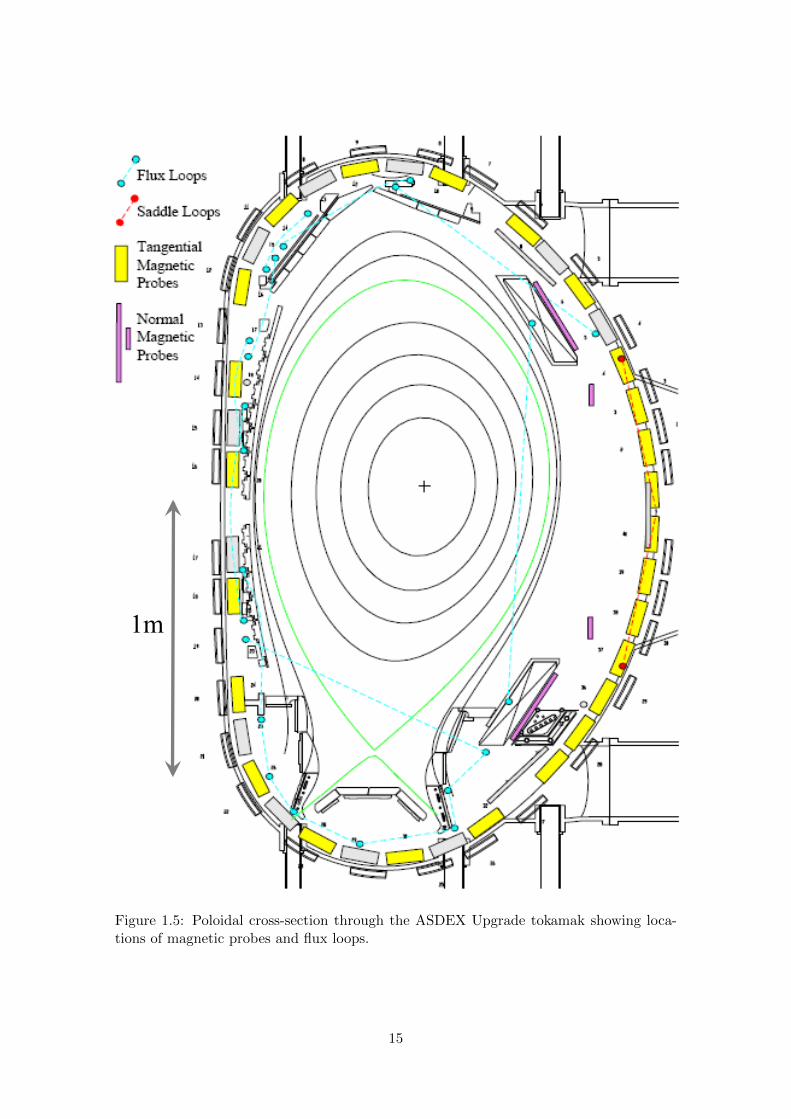
The work in this thesis was done on data from the ASDEX Upgrade tokamak based

in the Max Plank institute of Plasma Physics in Garching in Germany. Figure 1.5 shows

the poloidal cross section of the tokamak.

The Garching equilibrium code (see [28] and [29]) was used to generate a database con-

taining several thousand equilibria using the ASDEX Upgrade poloidal field coil configu-

ration (Figure 1.6). Each individual equilibrium is characterised by twelve input variables

corresponding to nine independently varying coil currents and three profile shape param-

eters to describe the toroidal current density in the plasma (since scaling all currents by

a constant factor does not alter the equilibrium, the plasma current is held constant at

1MA). The nine conductors comprise three pairs of coils (V1, V2 and V3 in Figure 1.6)

outside the main toroidal field coils, a pair of fast control coils (active stabilisers in Figure

1.6) inside the toroidal field coils and finally the upper and lower passive conductors inside

the vacuum vessel which form a single circuit producing a vertically stabilizing radial field

along the midplane.

14

Cross-section of ASDEX Upgrade showing locations of magnetic probes and flux loops

1m

Figure 1.5: Poloidal cross-section through the ASDEX Upgrade tokamak showing loca-tions of magnetic probes and flux loops.

15

Figure 1.6: The ASDEX Upgrade poloidal field coil system.

16

The flux due to the Ohmic field is virtually constant across the plasma cross-section

and thus, the Ohmic coil set was not considered for equilibrium generation. The current

profile parameters essentially determine the poloidal beta and internal inductance of the

plasma. The standard set of input paramters used for equilibrium generation are listed

below. The range of variation for each parameter is also listed.

Rmag = R coordinate of magnetic axis. Range: (1.2, 2.2).

Zmag = Z coordinate of magnetic axis. Range: (-0.6, 0.6).

C�

= Weighting of pressure derivative term in toroidal current density profile.

Range: (0.01, 2).

LLp

0 = Shape parameter of pressure derivative term in toroidal current density

profile. Range: (0, 2).

LLFF

0 = Shape parameter of poloidal current derivative term in toroidal current

density profile. Range: (0, 2).

V1u/Vlo = Ratio of lower to upper currents in V1 coils. Range: (0.2, 5).

V3o - V3u = Upper - lower current di↵erences in V3 coils. Range: (-0.2, 0.2).

PLun - PLob = Current di↵erence between lower and upper arms of passive con-

ductor. Range: (-0.2, 0.2).

CoIo = Current in upper fast control coil. Range: (-0.15, 0.15).

CoIu = Current in lower fast control coil. Range: (-0.15, 0.15).

V3o = Current in upper V3 coil. Range: (-0.15, 1.5).

V1u = Current in lower V1 coil. Range: (0, 4.6).

All coil currents, which are expressed as (number of coil windings ⇥ single-turn current),

are in units of the plasma current. During the generation of each equilibrium, the absolute

current is estimated using the plasma cross-sectional area and this is used to estimate the

absolute poloidal fields coil currents which are then checked against prescribed engineering

limits. If engineering limits are violated, the equilibrium is rejected. Note that the V2

coil currents are not specified, instead they are adjusted by the equilibrium solver at each

iteration to satisfy the condition that both components of the poloidal field vanish at the

magnetic axis.

17

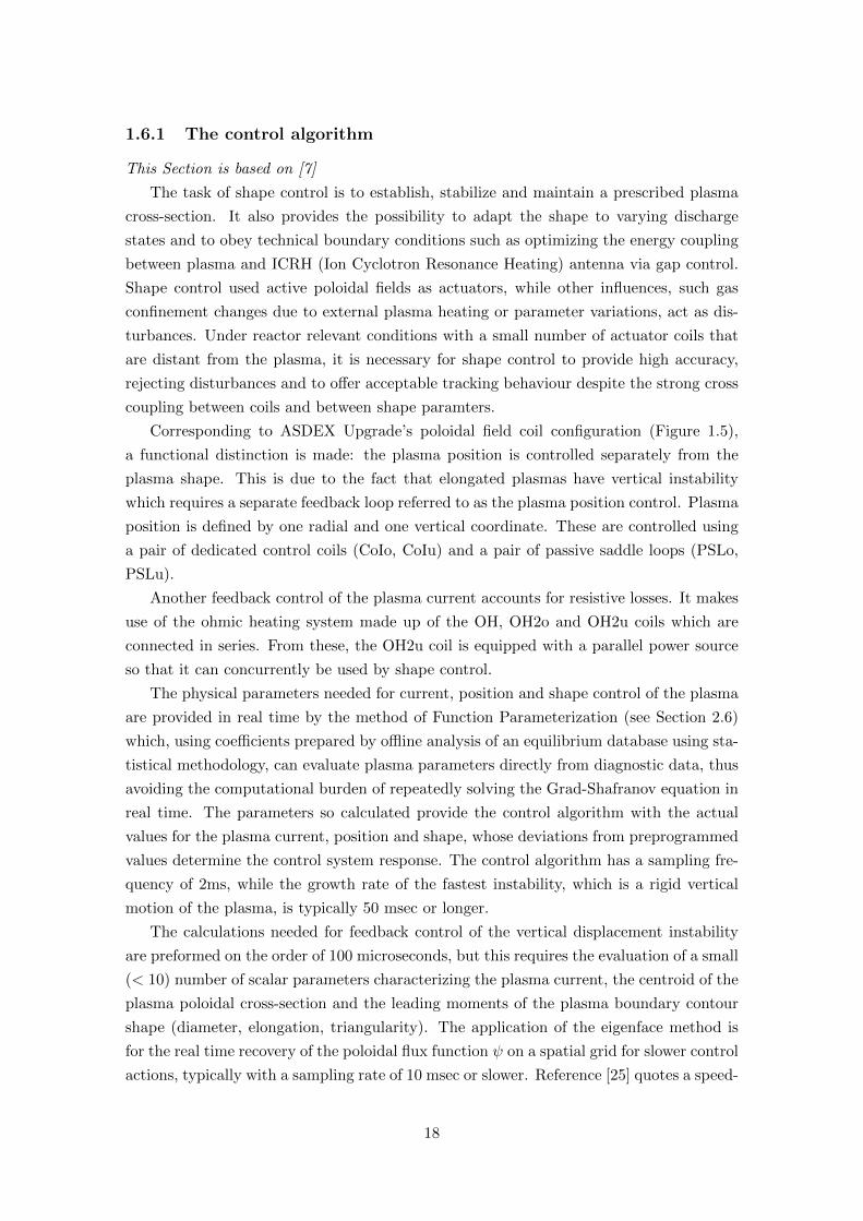
1.6.1 The control algorithm

This Section is based on [7]

The task of shape control is to establish, stabilize and maintain a prescribed plasma

cross-section. It also provides the possibility to adapt the shape to varying discharge

states and to obey technical boundary conditions such as optimizing the energy coupling

between plasma and ICRH (Ion Cyclotron Resonance Heating) antenna via gap control.

Shape control used active poloidal fields as actuators, while other influences, such gas

confinement changes due to external plasma heating or parameter variations, act as dis-

turbances. Under reactor relevant conditions with a small number of actuator coils that

are distant from the plasma, it is necessary for shape control to provide high accuracy,

rejecting disturbances and to o↵er acceptable tracking behaviour despite the strong cross

coupling between coils and between shape paramters.

Corresponding to ASDEX Upgrade’s poloidal field coil configuration (Figure 1.5),

a functional distinction is made: the plasma position is controlled separately from the

plasma shape. This is due to the fact that elongated plasmas have vertical instability

which requires a separate feedback loop referred to as the plasma position control. Plasma

position is defined by one radial and one vertical coordinate. These are controlled using

a pair of dedicated control coils (CoIo, CoIu) and a pair of passive saddle loops (PSLo,

PSLu).

Another feedback control of the plasma current accounts for resistive losses. It makes

use of the ohmic heating system made up of the OH, OH2o and OH2u coils which are

connected in series. From these, the OH2u coil is equipped with a parallel power source

so that it can concurrently be used by shape control.

The physical parameters needed for current, position and shape control of the plasma

are provided in real time by the method of Function Parameterization (see Section 2.6)

which, using coe�cients prepared by o✏ine analysis of an equilibrium database using sta-

tistical methodology, can evaluate plasma parameters directly from diagnostic data, thus

avoiding the computational burden of repeatedly solving the Grad-Shafranov equation in

real time. The parameters so calculated provide the control algorithm with the actual

values for the plasma current, position and shape, whose deviations from preprogrammed

values determine the control system response. The control algorithm has a sampling fre-

quency of 2ms, while the growth rate of the fastest instability, which is a rigid vertical

motion of the plasma, is typically 50 msec or longer.

The calculations needed for feedback control of the vertical displacement instability

are preformed on the order of 100 microseconds, but this requires the evaluation of a small

(< 10) number of scalar parameters characterizing the plasma current, the centroid of the

plasma poloidal cross-section and the leading moments of the plasma boundary contour

shape (diameter, elongation, triangularity). The application of the eigenface method is

for the real time recovery of the poloidal flux function on a spatial grid for slower control

actions, typically with a sampling rate of 10 msec or slower. Reference [25] quotes a speed-

18

up by a factor of 6 in evaluating (R,Z) relative to the existing Function Parameterization

method. For a 65 ⇥ 129 grid (already finer than the 40 ⇥ 70 grid presently used by FP)

and 50 eigenfaces, the number of multiplications is about p⇥NG

which for p=50 and NG

= 8385 is 429250 multiplications or 858500 floating point operations (multiplications and

additions). For a single core 3.2GHz clock Intel processor with 4 Floating point units and

hence 12.8 Gflops (with one flop per clock cycle assumed) the CPU evaluation time is just

67 microseconds. The actual evaluation speed would be limited by data bandwidth.

Figure 1.7 gives an overview of the control architecture. For shape control and load

compensation currently seven active coils are available. Correspondingly, five shape pa-

rameters can be concurrently controlled.

19

!

Figure 1.7: Control architecture

20

1.7 Equilibrium reconstruction

For more information, see [8 - 14]

Equilibrium reconstruction is a necessary diagnostic tool for determining the magnetic

field and current density of a tokamak discharge. Tokamak equilibria are reconstructed

in real time using an approximate solution to the Grad-Shafranov equation that best fits

the diagnostic measurements. Then a solution for the spatial distribution of the magnetic

field and current density is available in real time that is consistent with the plasma force

balance equation.

The availability in real time of plasma parameters related to the MHD (Magneto-

hydrodynamic) state is crucial for controlling tokamak experiments. In order to help

determine the plasma parameters quickly, Function Parameterization is used. Function

Parameterization (see Section 2.6) is a technique to provide real time construction of

system parameters from a set of diverse measurements. It consists of the numerical deter-

mination, by statistical regression on a database of simulated states, of simple functional

representations of parameters characterizing the state of a particular physical system,

where the arguments of the functions are statistically independent combinations of diag-

nostic raw measurements of the system.

The goal of this thesis is to apply eigenface analysis along side the techniques already

used for equilibrium reconstruction. Eigenface analysis is a technique that was developed

for the computer vision problem of human face recognition. Searching through literature

has not yielded any publications with the keywords “eigenface” and “plasma”. To our

knowledge, this thesis is the first instance of this technique being applied in plasma

physics. For more information on eigenfaces, see [15 - 22].

21

1.8 Outline of the Thesis

This thesis is concerned with the recovering of flux/current profiles from magnetic mea-

surements using Function Parameterization models based on singular value decomposi-

tion.

Chapter 2 reviews the statistical tools used in the thesis. Principal component analysis

and ordinary least squares regression are described. Function Parameterization, which is

the primary tool used in equilibrium reconstruction is introduced. Singular value decom-

position, which is used to compute Fourier moments of the flux/current, is also described.

A method for minimizing the e↵ects of measurement noise into the recovery from Func-

tion Parameterization is introduced. Eigenface analysis, the technique being applied to

equilibrium reconstruction in this thesis, is also described.

Chapter 3 uses the statistical methods introduced in Chapter 2 in the recovery of

the magnetic flux/plasma current profile from the Function Parameterization model and

the Fourier components. The training database which is used to aid in the development

of the Function Parameterization model is described. Singular value decomposition is

applied to the training database in order to obtain the corresponding eigenfaces. The

magnetic measurements then undergo principal component analysis and in conjunction

with the results from the singular value decomposition are used to generate the Function

Parameterization model.

Chapter 4 gives a conclusion to the thesis and describes the results obtained.

Appendix A gives a table of notations for the thesis. Appendix B gives the references

for the thesis. Appendix C gives the Mathematica code used in the project.

22

Chapter 2

Background Theory

Diagnosing the information about a tokamak plasma depends on measurements of the

poloidal flux and magnetic field. Each signal of the flux and magnetic field is treated as

a variable X, for which there exists a column vector of observations (or measurements)

x(n⇥1) consisting of the value of X for n randomly selected states. The individual obser-

vations are labelled with the index r. The di↵erent raw measurements are distinguished

by the subscripts i or j; thus for the variable Xi

, we have the column of observations xi

.

0

BBBBBBB@

V ariables �! X1 . . . Xi

. . . Xp

Observations x11 . . . x1i . . . x1p

#...

......

xr1 . . . x

ri

. . . xrp

......

...

xn1 . . . x

ni

. . . xnp

1

CCCCCCCA

.

Throughout this thesis, the convention of boldface lower case characters for data

vectors, boldface upper case characters for matrices will be used. The rth row of X which

consists of the rth observations on each of the p variables X1, ..., Xp

is denoted by xr

.

Like all unprimed vectors, xr

is manipulated as a column vector (p⇥ 1). A primed vector

or matrix represents the transposition of the corresponding unprimed entity, and primed

vectors are manipulated as row vectors.

2.1 A review of basic statistics

This Section is based on [23]

Let X(n⇥p) denote a data matrix, viewed as a random sample of n observations of

each of the p variables. The sample mean of the ith variable is

xi

=1

n

nX

r=0

xri

, i = 1, ..., p (2.1)

23

The p⇥1 vector of means,

2

664

x1...

xp

3

775 (2.2)

is called the sample mean vector.

The sample variance of the ith variable about it’s mean, xi

, is

sii

=1

n

nX

r=0

(xri

� xi

)2 =1

n(x

i

� xi

1)0(xi

� xi

1), (2.3)

where 1 is a column vectors of n ones and prime denotes transpose. The sample covariance

between the ith and jth variables is

sij

=1

n

nX

r=0

(xri

� xi

)(xrj

� xj

) =1

n(x

i

� xi

1)0(xj

� xj

1). (2.4)

The sample correlation coe�cient between the ith and jth variables is

rij

= sij

/psii

sjj

, (2.5)

which satisfies �1 rij

1 and rii

= 1. The p⇥p matrix S = (sij

) is called the

covariance matrix. It can be seen fromEqn. (2.4) that sji

= sij

, i.e. the covariance

matrix is symmetric and hence its own transpose: S0 = S.

To express S in matrix notation, simplify Eqn. (2.4) to get

sij

= xi

xj

� xi

xj

=1

nx0i

xj

� xi

xj

. (2.6)

The outer product of the vectors x and y is the matrix Z = xy0 with elements given by

zij

= xi

yi

. Hence we can write

S =1

nX0X� xx0. (2.7)

2.2 Singular Value Decomposition

This Section is based on [24, Section 2.9] and [25] and [15]

Singular Value Decomposition (SVD) is a set of techniques for dealing with matrices

that are singular (non-invertible, i.e. det(matrix)=0) or else numerically close to singular.

SVD methods are based on the following theorem of linear algebra: Any m⇥n matrix A

can be written as the product of an m⇥n column-orthogonal matrix U, an n⇥n diagonal

matrix W with positive or zero elements, and the transpose of an n⇥n orthogonal matrix

V:

24

A(m⇥n) = U(m⇥n)W(n⇥n)V0(n⇥n) (2.8)

If I(N) denotes the identity matrix with N diagonal elements, then U0U = I(m) and V0V

= I(n)The SVD of a matrix can also be written in the form (here m < n)

A(m⇥n) = U(m⇥m)⌃(m⇥n)V0(n⇥n), (2.9)

where ⌃ =diag(s1, s2, ..., sm) is the diagonal matrix of ordered singular values (s1 � s2 �... � s

m

� 0). The m columns of U and the n columns of V are called the left singular

vectors and right singular vectors of A respectively. The left singular vectors of A are

the eigenvectors of AA0 , the right singular vectors of A are the eigenvectors of A0A and

the non-zero singular values of ⌃ are the square roots of the non-zero eigenvalues of AA0

or A0A.

If n � m, then it can be time consuming to calculate the matrix V(n⇥n). It is possible

to calculate V from U(m⇥m). If S(n⇥n) = A0A and the eigenvectors of S are the right

singular vectors, V, then by the definition of eigenvectors

Svi

= A0Avi

= �i

vi

, (2.10)

where vi

is the ith eigenvector (of n eigenvectors) of A0A and �i

is the eigenvalue corre-

sponding to the eigenvector vi

. Instead, compute the eigenvectors of AA0 (i.e. U(m⇥m))

and premultiply by A0, i.e.

AA0ui

= �i

ui

(2.11)

) A0A(A0ui

) = �i

(A0ui

) (2.12)

) vi

= A0ui

(2.13)

) V(n⇥n) = A0(m⇥n)U(m⇥m). (2.14)

Note that the matrix V calculated in this manner is not normalized. As described in

Section 2.3 below, each row of A (with dimension n = NG

) can represent a 2D grid

(flattened into 1D) of ⌫ rows and µ columns where ⌫ ⇥ µ = NG

. In this case, the first m

columns of V, each represented as a ⌫ ⇥ µ matrix, constitute a set (Fj

) of m eigenfaces

of A. A small subset h ⌧ m of principal eigenfaces su�ces in practice to identify all

recoverable information from the matrix A. A is reconstructed as a linear combination

Ai

=hX

j=1

'i,j

Fj

, (2.15)

with Fourier-like amplitudes 'i,j

where 'i,j

= Fj

.Ai

(n⇥ 1) for the ith column of A.

25

2.3 Eigenfaces

This Section is based on [15 - 22]

Eigenfaces are a set of eigenvectors computed from the right singular vectors of a

matrix. They were first used in the computer vision problem of human face recognition.

It is a method used to extract the relevant information in a face image and encode it

as e�ciently as possible. In Eqn. (2.14), the set of the first m columns of V are the

eigenfaces of A. In this thesis, the method of using eigenfaces to analyse faces is used to

analyse magnetic flux and current density profiles from a tokamak plasma. This is done

by performing Singular Value Decomposition on a database of flux or current density

matrices, where each matrix is “flattened” into a high dimensional vector of length NG

where NG

is the grid dimension. For a matrix M of spatial dimensions NR

and NZ

, NG

is the product NR

⇥NZ

. Typically, a small number of singular vectors corresponding to

the largest singular values constitutes a parsimonious representation of M.

Each individual flux or current density matrix can be represented exactly in terms

of a linear combination of the eigenfaces. Each matrix can also be approximated using

only a (small) subset of eigenfaces i.e. those having the largest singular values and which

therefore account for a high fraction of the total variance within the database of matrices.

The best h eigenfaces span an h dimensional subspace of all possible images. The method

of using eigenfaces to analyse the data works as follows:

1. Read in matrix data from an existing equilibrium database.

2. Calculate the eigenfaces from the training database, keeping only the p eigenfaces

that correspond to the highest singular values.

3. These eigenfaces are then used in conjunction with the Fourier moments to recover

the 2D data.

26

2.4 Principal Component Analysis

This Section is based on [1, Section 2.2] and [26, Section 8]

Principal component analysis (PCA) is a mathematical procedure that uses an orthog-

onal transformation to convert a set of observations of possibly correlated variables into

a set of values of uncorrelated variables called principal components. Using the spectral

decomposition theorem, the covariance matrix S may be written in the form

S = �⇤�0, (2.16)

where � is the matrix of orthogonal eigenvectors of S and ⇤ is a diagonal matrix of

the eigenvalues of S, �21 � �22 � ... � �2p

� 0. If S is positive semi-definite, it has no

negative eigenvalues. The notation �2 is used because the eigenvalues are synonymous

with variance. The covariance matrix is used in this thesis as opposed to the correla-

tion matrix because all the signals used are physically similar and thus have the same

dimension and they also have similar experimental errors. Thus the covariance matrix is

preferred because every signal is treated on the same footing. The principal component

transformation is defined by the rotation

�r

= �0(xr

� x), r = 1, ..., n. (2.17)

Eqn. (2.17) can be written as

�ri

= �0i

(xr

� x) = (xr

� x)0�i

=pX

j=0

(xrj

� xj

)�ji

. (2.18)

This gives

�i

= (X� 1x0)�i

, (2.19)

where �i

is the column of observations of the “transformed measurements” �i

, where

�i

=pX

j=0

�ji

(Xj

� Xj

). (2.20)

�i

is a linear combination of the physical measurements X1, ..., Xp

whose coe�cients are

the elements of the ith eigenvector, �i

. The covariance of �i

and �j

is

sij,�

=1

n�0i

�j

= �0i

1

n(X� 1x0)0(X� 1x0)�

j

= �0i

S�j

= �2�ij

. (2.21)

The properties of PCA are as follows: (i) the average value of each principal component is

zero: �i

= 0 , (ii) the variance of the ith principal component is given by the ith eigenvalue:

sii,�

= �2i

, (iii) the principal components �i

are uncorrelated linear combinations of the

original variables Xi

: sij,�

= 0, j 6= i. Writing the n⇥p observation matrix as �, we have

27

� = (X� 1x0)�. (2.22)

Hence, the covariance matrix for � becomes

S�

=1

n�0� = �0 1

n(X� 1x0)0(X� 1x0)� = �0S� = ⇤, (2.23)

which is the diagonal matrix of the eigenvalues of S.

2.5 Multiple Linear Regression

This Section is based on [1, Section 2.4] and [26, Section 6]

Consider the model defined by

y = X� + ✏, (2.24)

where y(n⇥ 1) is a vector of n observations on a dependent variable, X(n⇥ (p+ 1)) is a

known matrix of n observations on each of p predictor variables together with a constant

column of ones to allow for an overall mean, �((p + 1) ⇥ 1) is a vector of unknown

regression coe�cients and ✏(n ⇥ 1) is a vector of unobserved random disturbances with

zero expectation value, but possibly correlated with each other with a covariance matrix

V(✏) = ⌃. The columns of X are assumed to be linearly independent. We wish to solve

for that � which minimizes the residual sum of squares defined as

RSS = (y �X�)0(y �X�). (2.25)

Defining

@f(X)

@X=@f(X)

@xij

, (2.26)

where xij

is the element of X in row i, column j, gives the following result

@a0x

@x= a, (2.27)

@x0Ax

@x= 2Ax, (2.28)

@x0Ay

@x= Ay, (2.29)

Expanding and di↵erentiating Eqn. (2.25) with respect to the solution vector � gives

� = (X0X)�1X0y, (2.30)

where the hat symbol indicates that this is an estimate. Since the second derivative matrix

of equation(2.25), 2X0X � 0(C = X0X is a symmetric real matrix and hence | C |� 0)

28

this is indeed the minimum RSS, or “least squares” solution.

Using the linearity property of the expectation value,

E(Ax+ b) = AE(x) + b, (2.31)

(where A and b are constant) gives

E(�) = (X0X)�1X0(� + E(✏)) = �. (2.32)

2.6 Function Parameterization

This Section is based on [1, Section 2.6]

2.6.1 Basic Concepts

The method of Function Parameterization (FP) consists of the numerical determination,

by statistical regression on a database of simulated states, of simple functional represen-

tations of parameters characterizing the state of a particular physical system, where the

arguments of the functions are statistically independent combinations of diagnostic raw

measurements of the system whose geometry is fixed.

A classical physical system is considered, of which G denotes a typical state. The

system may have any number of degrees of freedom, but interest will be restricted to

a characterization by m intrinsic real parameters, represented collectively by a point

g 2 <m. In the experimental situation, g is to be estimated from the readings of p

measurements, represented by a point x 2 <p. It is assumed that g is completely specified

by G, but that x may be a stochastic function of G, the stochasticity being due to random

errors in the measurement process. The notation g = g(G) and x = x(G) will be used.

The aim of the FP is to obtain some reasonably simple function, F : <p ! <m, such

that for any state G the associated g(G) and x(G) satisfy g = F(x) + ✏ for a su�ciently

small error term ✏. The unknown coe�cients in F are then determined by analysis of a

database containing the values of the paramters gr

and of the measurements xr

corre-

sponding to n simulated states Gr

(1 r n). The use of multivariate statistical analysis

can be used for solving this problem since it is function fitting over scattered data.

2.6.2 The data base

First, a database is generated using a code C. This code must be suited to compute

possible states of the physical system over the whole of the system’s regime and must also

contain a model for the measurements. The code will take certain numerically convenient

parameters as input and produce g and x as results. The input parameters are varied,

and for each successful calculation, indexed by r, the values gr

and xr

are saved. Using

29

FP, the aim is to obtain a direct and much simpler connection between measurements

and physical parameters, without sacrificing too much accuracy.

2.6.3 Dimension reduction

Since the dimensionality p of the space of the measurements may be of the order of several

tens, and since a linear representation for g in terms of x is not expected to su�ce, the

dimensionality of the space of functions with which the physical parameters will be fitted

will be very large. A polynomial of degree l has ⇠ pl/l! degrees of freedom for each physical

parameter. Therefore, it is necessary to first reduce the number of independent variables

(the components of x). Secondly, the multicollinearity will be reduced between the data

points which will improve the conditioning of the regression problem. Multicollinearity

is likely to be present whenever the number of measurements is much larger than the

number of independently measurable physical parameters.

A method for dimension reduction and elimination of multicollinearity that is widely

used in statistics is based in principal component analysis. From the n suitably scaled

pseudo measurements xr

, each of which is a point in <p, the sample mean x = n�1Pr

xr

and the p⇥p sample dispersion matrix

S = n�1nX

r=0

(xr

� x)(xr

� x)0 (2.33)

are calculated. S is symmetric and positive semi-definite. An eigenanalysis yields p eigen-

values, �21 � ... � �2p

� 0, with corresponding orthomormal eigenvectors �1, ..., �p. Any

measurement vector xr

may be resolved along these eigenvectors to obtain a set of trans-

formed measurements, �ri

= �0i

(xr

� x). This is the principal component transformation,

and the �ri

are the principal components of the measurement vector xr

.

The transformed measurement columns, �i

(1 i p) are linearly independent within

the sample, and have zero mean and standard deviation �i

. One of the aims, the reduc-

tion of multicollinearity, has therefore been achieved, but if all of the p components are

retained, the dimensionality has not been reduced. One of the properties of PCA is that

the most significant information will be contained in the first few principal components,

�i

; 1 i pR

, where pR

is the number of retained principal components.

An important consideration in choosing pR

is the sensitivity of the Function Parame-

terization to raw measurement noise. For this analysis, assume that the regression model

is linear in the principal components. This does not cause a loss of generality since second

degree terms are formally treated as additional linear terms in the regression. Denote the

FP for a parameter Y as Y =pRPi=1

�i

�i

where � is the vector of estimates. Then the

variance of a particular estimate yr

can be written as

V ar(yr

) =�2y

n

pRX

i=1

�2ri

�2i

+ �2pRX

i=1

�2 (2.34)

30

denoting the two contributions to Var(yr

) as Vfit

and Vran

respectively. �2y

is defined

asP

r

(yr

� yr

)/(n � pr

) and is the FP regression mean square fitting error. Generally,

random noise in the raw measurements makes the dominant contribution to the prediction

variance for well recovered FP parameters. For poorly recovered parameters, the lack of

fit variance is comparable to the random noise variance. This means that the first term

in Eqn. (2.34) can be ignored for well recovered parameters.

2.6.4 Use of incremental signal to noise ratio as selection criterion for

the Principal Components

The method used to decide the number of principal components to be included in the FP

regression, pR

, is provided by the concept of incremental signal to noise ratio. Incremental

signal refers to the improvement in the explained variance of the regression parameter due

to the extra term in the prediction equation. The incremental noise is the increase in the

noise variance caused by the propagation of raw measurement noise in the new term.

Denoting the standard deviation of Y by sy

=q

1n

Pr

(yr

� y)2, the retention criterion

for the new term is defined to be the signal to noise ratio exceeding unity, i.e.

�s2y

�Vran

� 1. (2.35)

Linear, bilinear and quadratic principal component (PC) combinations will be consid-

ered and the cut-o↵ criterion in each case will be derived. For linear PC’s, the variance

contributed by the term �a

�a

is given by

�lin

s2y

= V ar(�a

�a

) = �2a

�2a

. (2.36)

Since the noise variance contribution is �lin

Vran

= �2a

�2, the inclusion condition for the

linear PC variable,�a

, is

�2a

� �2. (2.37)

For the quadratic PC term �aa

(�2a

� �2a

), the condition is

�2a

� �2(1 +p2), (2.38)

and the condition for the bilinear term is

�2a

�2b

� �2(�2a

+ �2b

) + �4. (2.39)

2.6.5 Optimal suppression of signal noise by using filtering techniques

Even though the regressions are made with noiseless predictor variables, the evaluation

of the Function Parameterization will be subject to raw measurement errors. This is

31

taken into account by introducing noise to the variables before performing the regression.

Consider the model

y = y1+ (X+�)�, (2.40)

where �(n⇥p) is a matrix of error terms from p uncorrelated error variables �i

; 1 i p

with �i

⇡ N(0,�). To solve this, seek the � which minimises the residual sum of squares

defined as

RSS = (y � (X+�)�0)(y � (X+�)�). (2.41)

The solution to this equation is the same as that of Eqn. (2.25) and the extremum

condition is

(X+�)0(X+�)� = (X+�)0y. (2.42)

Assuming that there is no correlation between the errors and the X or Y variables, i.e.

the matrix �X and the vector �0y vanish, gives the estimate for �

� = (X0X+ n�2I)�1X0y. (2.43)

For principal component regression, where X is replaced by �, the solution simplifies to

� = (diag(n�2i

) + n�2I)�1�0y (2.44)

= diag(n�2i

+ n�2)�1�0�(�0�)�1�0y (2.45)

= diag(1/(n�2i

+ n�2))diag(n�2i

)�(0) (2.46)

= diag(�2i

/(�2i

+ �2))�(0), (2.47)

where �(0) is the ordinary least squares solution. Therefore, it can be seen that the �

dependence for the noise-optimized regression coe�cients is

�i

(�) =�2i

�2i

+ �2�(0) (2.48)

=�i

(0)

1 + �2/�2i

. (2.49)

The damping factor, �2i

/(�2i

+�2), can now be used to determine the cut-o↵ criteria for the

various PC variables. For linear PC’s, the incremental variance contributed by the term

�a

(�) is given by Eqn. (2.36) . The mean squared error (MSE) in the linear component

is then

32

�lin

MSE = h(�a

(�)�a

+ Ea

� �a

(0)�a

)2i (2.50)

= �2a

(0)h�2a

+ 2�a

Ea

+ E2a

(1 + �2/�2a

)2� 2

�2a

+ �a

Ea

1 + �2/�2a

+ �2a

i (2.51)

= �2a

(0)(�2a

+ 0 + �2

(1 + �2/�2a

)2� 2

�2a

+ 0

1 + �2/�2a

+ �2a

) (2.52)

= �2a

(0)(��2

a

1 + �2/�2a

+ �2) (2.53)

=�2a

(0)�2

1 + �2/�2a

. (2.54)

The inclusion condition is that Eqn. (2.36) must be greater than Eqn. (2.54), i.e.

�2a

(0)�2a

>�a

(0)�2

1 + �2/�2a

. (2.55)

Dividing across by the � term and rearranging gives

�2a

+ �2 > �2. (2.56)

Since �2a

is always positive, the above expression is true for all values of �a

. Therefore,

there is no cut-o↵ point for removing linear PC variables from the filtered FP regression.

Repeating the above steps for the quadratic and bilinear regression coe�cients gives:

�aa

(�) =�aa

(0)

(1 + �2/�2a

)2, (2.57)

�ab

(�) =�(0)

(1 + �2/�2a

)(1 + �2/�2b

). (2.58)

33

2.7 Error analysis

2.7.1 The percentage error

Error analysis in this thesis was done by calculating the percentage error of the recovered

data. Take an m ⇥ 1 vector a and a vector ar

that has been recovered using Function

Parameterization. Then calculate the rms value (rmsv) of the elements of a

rmsv =p(a0a)/m (2.59)

and the rms error (rmse) adjusted for degrees of freedom

rmse =p

((a� ar

)0(a� ar

))/(m� b), (2.60)

where b is the number of coe�cients in the model used to recover ar

. Then, the percentage

error is:

P = 100rmse

rmsv. (2.61)

For n vectors, the percentage error is an n⇥ 1 vector Pi

where 1 i n and

Pi

= 100rmse

i

rmsvi

. (2.62)

2.7.2 An alternative method of calculating the percentage error

An alternative method of calculating the percentage error follows. The % error of is

calculated as a function of the number of eigenfaces used to recover it. Let si

denote the

value of the ith singular value, pi

, the % recovery error of the ith Fourier amplitude and

h be the number of eigenfaces used to recover the flux. Then a representative value

would be: (assuming �j

⇡ sj

)

(R,Z) =hX

i

�i

Fi

. (2.63)

The squared modulus of is then

| |2 =

hX

i=1

�i

Fi

!00

@hX

j=1

�j

Fj

1

A (2.64)

=hX

i,j

�0i

�j

Fi

Fj

(2.65)

=hX

i=1

�2i

, (2.66)

34

since

Fi

Fj

= 0, i 6= j, (2.67)

= 1, i = j. (2.68)

Adding noise to � gives

| ⌫

|2 =hX

i,j

(�i

+ ⌫i

)(�j

+ ⌫j

)Fi

Fj

, (2.69)

where ⌫i

denotes the noise that was added to �i

. Invoking again F 0i

Fj

= 0; i 6= j, and

assuming the noise is independent of which � it is added to,

| ⌫

|2 =hX

i=1

(�i

+ ⌫i

)2 (2.70)

=hX

i=1

h�2i

i+ 2h�i

⌫i

i+ h⌫2i

i. (2.71)

Since � and the noise are uncorrelated and assuming �i

⇡ si

, this gives

| ⌫

|2 =hX

i=1

(s2i

+ �2i

), (2.72)

where �2i

is the noise variance of the ith Fourier amplitude.

The % error, denoted by pi

, is (see Eqn. (2.61))

pi

= 100�i

si

(2.73)

=) �2i

= s2i

⇣ pi

100

⌘2(2.74)

=) | ⌫

|2 =hX

i=1

s2i

+ (pi

100)2s2

i

. (2.75)

The R2 value of a regression model is defined as the fraction of the variance due to

regression model over the variance in the data. An R2 statistic can be constructed by

equating the variance of the exact �i

with that explained by the regression model and the

variance of the noisy �i

with the total variance:

35

R2 =

Ph

i

s2iP

h

i

(s2i

+ ( pj

100)2s2

i

)(2.76)

=| |2

| n

|2 (2.77)

=1

1 +Ph

i (pi100 )

2s

2iPh

i s

2i

. (2.78)

Thus, the overall % error prediction (E) for the recovered value is: (denotingPhi (

pi100 )

2s

2iP

i s2 as x)

E = 100p1�R2 (2.79)

= 100

r1� 1

1 + x(2.80)

= 100

vuuuut

Phi e

2js

2jPh

i s

2i

1 +Ph

i e

2i s

2iPh

i s

2i

, (2.81)

where ei

= pi

100 is the fractional recovery error for the ith Fourier Amplitude. Now let

t2i

=s

2iPhi s

2i

be the jth squared singular value as a fraction of the total variance. Thus the

overall % error predicted for is

E = 100

vuutP

h

i

e2i

t2i

1 +P

h

i

e2i

t2i

. (2.82)

It can be assumed thatP

h

i

e2i

t2i

⌧ 1. This can be done since ei

is a percentage divided

by 100 and thus less than 1 and ti

= siPhi si

⌧ 1 for large values of i. If these apply, then

E = 100

vuuthX

i

e2i

t2i

. (2.83)

The percentage error calculated thus far is the error in the flux recovered using p

eigenfaces. But it can be useful to calculate the percentage error after a partial recovery

using k eigenfaces. This can show how the recovery improves as a function of the number

of eigenfaces used in the recovery.

R2k

=

Pk

i=1 s2iP

n

i=1 s2i

(1 + e2j

)(2.84)

36

=) 1�R2k

=

Pn

i=1 s2i

+P

n

i=1 e2i

s2i

�P

k

i=1 s2iP

n

i=1 s2i

(1 + e2i

)(2.85)

=

Pn

i=k+1 s2i

+P

n

i=1 e2i

s2iP

n

i=1 s2i

(1 + e2i

). (2.86)

And, finally, the overall % error in after a recovery using k eigenfaces is

Ek

= 100q1�R2

k

. (2.87)

37

Chapter 3

Reconstruction of 2D MHD

equilibrium states using database

training methods

Equilibria generated in the ASDEX Upgrade tokamak fall into one of four categories.

These are: (1) the inner limiter where the plasma boundary is in contact with the inner

limiter, (2) the outer limiter where the plasma boundary is in contact with the outer

limiter, (3) upper X-point where the plasma boundary is a magnetic seperatrix (i.e. it

is not in contact with any of the limiters) with the X-point as the highest point on the

boundary and (4) lower X-point where the plasma is a magnetic seperatrix with the X-

point as the lowest point on the boundary. Any X-point plasma can become a limiter

plasma if it moves inwards or outwards enough that it rubs against the inner or outer

limiter. In this thesis, the Lower X-point category was analysed.

3.1 The training database

This thesis is primarily concerned with recovering the magnetic flux and the magnetic

current profile from magnetic data taken during experiments using the ASDEX Upgrade

tokamak. A training database of the flux or the current was used to aid in the development

of a Function Parameterization model for the recovery of the flux or current. The training

database is represented as a matrix M of Neq

rows and NG

= NR

⇥ NZ

columns where

Neq

is the number of equilibria (or states) in the database, NR

and NZ

are the grid

dimensions, and each row of M consists of all NG

flux or current values for one state. The

grid size for the training database used in this thesis was NR

⇥NZ

= 129⇥ 257 giving M

dimensions of Neq

⇥NG

= 2546⇥33153 for Neq

= 2546. The current profile was generated

from the magnetic flux using the Grad-Shafranov equation (Eqn. (1.38)). Fig 3.1 shows

contour plots of the magnetic flux of the plasma measured for some equilibira. Figure

3.2 shows contour plots of the current density in the plasma for the same equilibria. The

38

plots also include the contour of the tokamak first wall and show the in-vessel passive

conductors which act as a brake on the unstable vertical motion of the plasma.

The magnetic flux data for the training database was provided by Dr. Patrick Mc-

Carthy (see [28] and [29] for a description of the generation of a database of randomly

selected equilibria) and the current profile was calculated from the magnetic flux using

the Grad-Shafranov equation. Contour plots were made in the notebook (a file written

using Mathematica) cplot.nb (see Appendix C) which is based o↵ code written by Dr.

Patrick J. McCarthy.

39

Figure 3.1: Contour plots of some magnetic flux equilibria. Red denotes a maximum andblue denotes a minimum.

40

Figure 3.2: Some current density equilibria, corresponding to the flux plots in the previousfigure. Red denotes a maximum and blue denotes a minimum.

41

3.2 Singular Value Decomposition of the training database

3.2.1 SVD of the magnetic flux

In the notebook SVD.nb (see Appendix C), singular value decomposition was performed

on the training database of magnetic flux to get the eigenfaces and Fourier moments of

the flux. As stated in Section 3.1, the magnetic flux was in the form of a matrix with Neq

rows and NG

= NR

⇥ NZ

columns where Neq

is the number of states in the database,

NR

and NZ

are the grid dimensions. Again, Neq

= 2546, NR

= 129, NZ

= 257 and

NG

= 33153. Figures 3.3 and 3.4 show log10 plots of the singular values of the magnetic

flux respectively. As can be seen, the size of the singular values decrease fairly quickly,

s100 is already a factor of 1 ⇥ 10�5 smaller than s1. This means that the weight of the

corresponding eigenfaces in the reproduction of the magnetic flux decrease rapidly and

hence only a small number of eigenfaces are needed in the reproduction and it will be

shown later that 100 eigenfaces is well beyond the limits of identifiability.

Figures 3.5 and 3.6 show some of the eigenfaces computed for the magnetic flux. As

stated in section 2.3, only a few eigenfaces are needed in order to recover the magnetic

flux. This can be confirmed by the similarity in the first two eigenfaces (which have the

largest eigenvalues and hence have a larger weight in the reproduction of the flux) to some

of the magnetic flux plots in Fig 3.1. The further eigenfaces have lower eigenvalues and

hence a lower weight in the reproduction but can be considered to be “corrections” to the

reproduction.

42

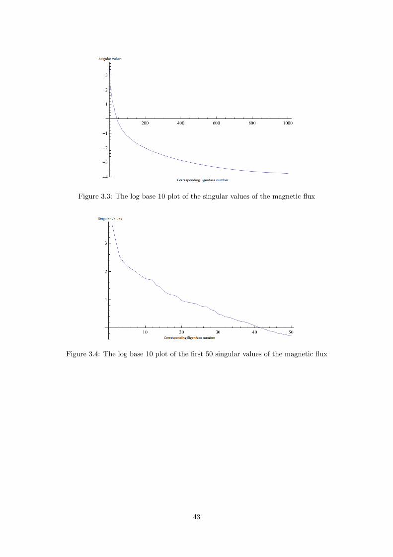
Figure 3.3: The log base 10 plot of the singular values of the magnetic flux

Figure 3.4: The log base 10 plot of the first 50 singular values of the magnetic flux

43

Figure 3.5: Contour plots (versus R and Z) of (flux) eigenfaces 1-6. Red denotes amaximum and blue denotes a minimum.

44

Figure 3.6: Contour plots (versus R and Z) of (flux) eigenfaces 8, 18, 23, 30, 36 and 40.Red denotes a maximum and blue denotes a minimum.

45

3.2.2 SVD of the current profile

Similarly to the magnetic flux, singular value decomposition was also done (in the note-

book SVD.nb) on the current profile to aid in its recovery. Prior to doing SVD on the

current profile, the current flowing in the passive conductors was zeroed so that only the

current in the plasma was considered. Figures 3.7 and 3.8 show log10 plots of the singular

values of the current density. As can be seen, the size of the singular values decrease fairly

quickly, s100 is 100 times smaller than s1. This fall is significant but not as dramatic as the

decrease seen in the singular values computed for the magnetic flux. This means that the

weight of the corresponding eigenfaces in the reproduction of the magnetic flux decrease

rapidly and hence only a small number of eigenfaces are needed in the reproduction.

Figures 3.9 and 3.10 show some of the eigenfaces computed for the current density.

As stated in section 2.3, only a few eigenfaces are needed in order to recover the current

density. This can be confirmed by the similarity in the first eigenface (which have the

largest eigenvalue and hence has a larger weight in the reproduction of the flux) to some

of the magnetic flux plots in Fig 3.2. The further eigenfaces have lower eigenvalues and

hence a lower weight in the reproduction but can be considered to be “corrections” to the

reproduction. Some of the eigenfaces can be seen to have some “fuzz” outside the plasma.

This is very low valued noise and as such is inconsequential for further calculations.

46

Figure 3.7: The log base 10 plot of the singular values for the current density

Figure 3.8: The log base 10 plot of the singular values for the current density

47

Figure 3.9: Contour plots (versus R and Z) of (current) eigenfaces 1-6. Red denotes amaximum and blue denotes a minimum.

48

Figure 3.10: Contour plots (versus R and Z) of (current) eigenfaces 8, 18, 23, 30, 36 and40. Red denotes a maximum and blue denotes a minimum.

49

In the notebook SVD.nb (see Appendix C), code was written that does the singular

value decomposition (as described in Section 2.2) by first calculating A’A (where A is

the dataset and A’ is its transpose) and then using Mathematica’s Eigensystem function

to get the eigenvectors and eigenvalues of A’A. These eigenvectors are the left singular

vectors and the right singular vectors are calculated from the left singular vectors and A

using Eqn. (2.14).The eigenfaces are a subset of the right singular vectors. Then, the

Fourier-like amplitudes were calculated as a product of the eigenfaces and A.

3.3 Principal component analysis of magnetic measurements

Prior to using the magnetic data from the ASDEX upgrade tokamak experiments, prin-

cipal component analysis must be done on the data to reduce dimensionality and remove

multicollinearities as described in Section 2.3. The 65⇥ 65 covariance matrix for the flux

and field measurements was constructed. Eigendecomposition of this covariance matrix

gives 65 eigenvectors and their corresponding eigenvalues. The database standard devi-

ations of the magnetic data and the square roots of the eigenvalues, which correspond

to the standard deviations of the transformed measurements, are plotted in figure 3.11.

Figure 3.12 shows the log10 plot of the square root of the eigenvalues.

Figure 3.11: The database standard deviations of the magnetic data (blue) and the squareroot of the eigenvalues (red) of the 65⇥65 measurement covariance matrix.

50

Figure 3.12: A log, base 10 plot of the square root of the eigenvalues of the 65⇥65measurement covariance matrix

The standard deviations of the measurements show how strongly the value of each

simulated magnetic signal varies over the N cases in the database. Ignoring signals 17

and 23 (which are always zero-valued because they are actually physically not present

but were included to preserve the natural sequence of the rest of the signals), the stan-

dard deviation of the signals lies in the range 0.01 - 0.3. The variation of a signal in the

database is a direct measure of information value (no variation means the signals carries

no information) and no signal can therefore be discarded as being of negligibly small

variation compared to other signals. Performing PCA on the measurements gives eigen-

vectors and the corresponding eigenvalues where the square root of the eigenvalue is the

standard deviation of the transformed signal defined as the dot product of the eigenvector

vector with the measurement vector. This allows a dramatic reduction in the number of

transformed signals needed to be retained, because the majority of the eigenvalues are

tiny compared to the first few eigenvalues. This can be seen in Fig 3.12 as the square

root of eigenvalues 30 and above are at least 1000 times smaller than the square root of

the first eigenvalues. For the standard deviations in Fig 3.11, there is only a factor of 30

between the largest and smallest deviations of the original signals.

The principal components were then calculated using

� = (X� 1x0)� (3.1)

51

where X denotes the magnetic data that is undergoing principal component analysis and

� denotes the eigenvectors of the covariance matrix of X.

The magnetic data was provided by Dr. Patrick McCarthy (see [28] and [29] for a

description of the generation of a database of randomly selected equilibria) and he wrote

the code involved in inputting it which I added to the notebook regfp.nb (see Appendix

C). While it is possible to find the principal components using Mathemactica’s Principal

Components function, I calculated the principal components using Eqn. (3.1) which

allowed the calculation of the eigenvalues and standard deviation used in Figures 3.11

and 3.12.

3.4 Recovering the Fourier moments using Function Pa-

rameterization

The jth (1 < j < h, where h is the number of eigenfaces and Fourier moments used in the

recovery) Fourier moment �j

was regressed using a quadratic model with (m+1)(m+2)/2

terms and the intercept, linear and quadratic coe�cients were saved, where m is the

number of principal components of the magnetic data that were retained. A Function Pa-

rameterization model with m = 26 magnetic principal components resulting in a quadratic

regression model size of 378 terms was used to regress the Fourier moments. The number

26 was chosen because the square root of the 26th eigenvalue (p8.8⇥ 10�7 = 0.938mT)

is similar in magnitude to the noise level in ASDEX Upgrade (1mT), giving a reasonable

signal to noise ratio.

The coe�cients that were calculated from the Function Parameterization were then

used in conjunction with the magnetic data to recover the Fourier moments using the

following formula:

�j

= aj

+mX

r=1

brj

�r

+mX

r=1,s=r

crsj

�r

�s

for j = 1, 2,..., h.

These recovered Fourier moments were then compared with the original moments

by calculating the recovery rms error as a percentage of the rms magnitude using Eqn.

(2.62). The recovery of the Fourier moments was also perturbed by adding small amounts

of random noise to the data before doing the Function Parameterization. Since data taken

from experiments will have noise, noise filtering is implemented by adding noise before

the Function Parameterization step. Results for the recovery of Fourier moments 1-100

for the flux are presented in Figure 3.13 for various noise levels (see figure caption).

Fig 3.13 shows the quality of the recovery in the form of the root mean square recov-

ery error of the Fourier moments (adjusted for degrees of freedom loss) expressed as a

percentage of the root mean square value of the Fourier moment. A 100 % recovery error

means that the corresponding Fourier moment is unidentifiable. Looking at the graph, it

can be seen that, for the first 10 or so Fourier moments, the recovery errors are below 10%

52

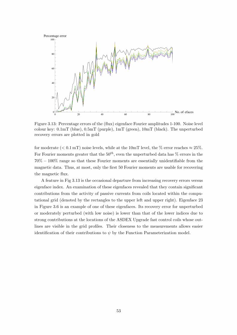
0 20 40 60 80 100No. of efaces0

20

40

60

80

100Percentage error

Figure 3.13: Percentage errors of the (flux) eigenface Fourier amplitudes 1-100. Noise levelcolour key: 0.1mT (blue), 0.5mT (purple), 1mT (green), 10mT (black). The unperturbedrecovery errors are plotted in gold

for moderate (< 0.1mT) noise levels, while at the 10mT level, the % error reaches ⇡ 25%.

For Fourier moments greater that the 50th, even the unperturbed data has % errors in the

70%� 100% range so that these Fourier moments are essentially unidentifiable from the

magnetic data. Thus, at most, only the first 50 Fourier moments are usable for recovering

the magnetic flux.

A feature in Fig 3.13 is the occasional departure from increasing recovery errors versus

eigenface index. An examination of these eigenfaces revealed that they contain significant

contributions from the activity of passive currents from coils located within the compu-

tational grid (denoted by the rectangles to the upper left and upper right). Eigenface 23

in Figure 3.6 is an example of one of these eigenfaces. Its recovery error for unperturbed

or moderately perturbed (with low noise) is lower than that of the lower indices due to

strong contributions at the locations of the ASDEX Upgrade fast control coils whose out-

lines are visible in the grid profiles. Their closeness to the measurements allows easier

identification of their contributions to by the Function Parameterization model.

53

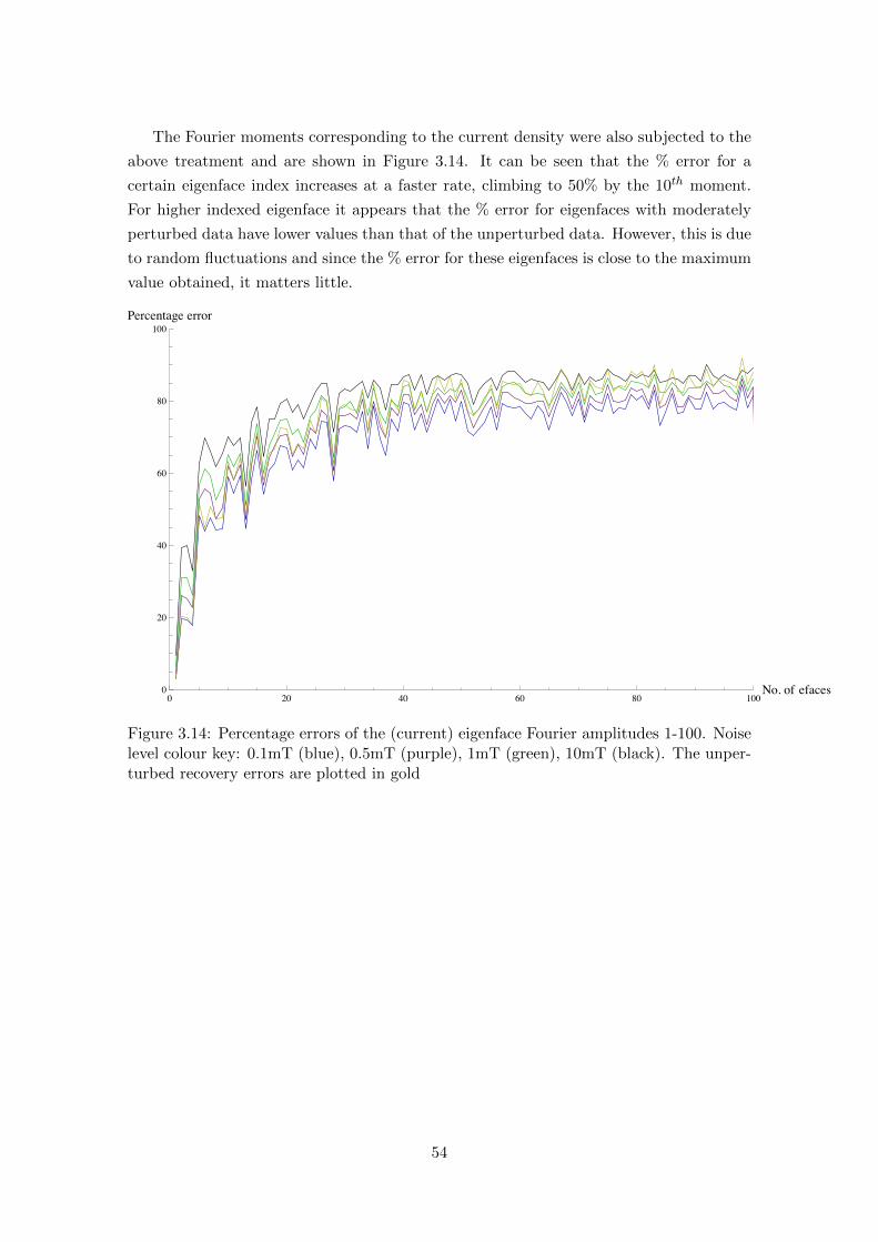
The Fourier moments corresponding to the current density were also subjected to the

above treatment and are shown in Figure 3.14. It can be seen that the % error for a

certain eigenface index increases at a faster rate, climbing to 50% by the 10th moment.

For higher indexed eigenface it appears that the % error for eigenfaces with moderately

perturbed data have lower values than that of the unperturbed data. However, this is due

to random fluctuations and since the % error for these eigenfaces is close to the maximum

value obtained, it matters little.

0 20 40 60 80 100No. of efaces0

20

40

60

80

100Percentage error

Figure 3.14: Percentage errors of the (current) eigenface Fourier amplitudes 1-100. Noiselevel colour key: 0.1mT (blue), 0.5mT (purple), 1mT (green), 10mT (black). The unper-turbed recovery errors are plotted in gold

54

It is possible to increase the accuracy of the results by only considering equilibria in

which the plasma is near the measurement coils and taking the 1000 closest equilibria.

The results of this are shown in Fig 3.15. This typically resulted in a 20% drop in the %

err for the current eigenfaces.

0 20 40 60 80 100No. of efaces0

20

40

60

80Percentage error

Figure 3.15: Percentage errors of the (current) eigenface Fourier amplitudes 1-100 withthe 1000 equilibria closest to the contour of measurement coils. Noise level colour key:0.1mT (blue), 0.5mT (purple), 1mT (green), 10mT (black). The unperturbed recoveryerrors are plotted in gold

The Function Parameterization (and subsequent analysis) was done in the notebook

regfp.nb (see Appendix C). In order to do the Function Parameterization, I made a

quadratic model from the principal components and then used Mathematica’s Least-

Squares function with the quadratic model and the Fourier amplitudes as inputs. This

outputs the fit parameters that can be used to recover the Fourier amplitudes from mag-

netic data. The code to compute the percentage errors in the recovered Fourier amplitudes

was written by Dr. Patrick McCarthy and random noise was added to the magnetic data

prior to the Function Parameterization and again prior to the recovery in order to test

the e↵ectiveness of noise suppression.

55

3.5 E↵ectiveness of noise suppression

As stated in Section 2.6.5, it is possible to reduce the e↵ect of noise in the measurements

by adding noise to the data before performing the regression of the Fourier moments.

First, noise was added to the magnetic data and the principal component values were

recomputed as the inner product of the stored, exact eigenvectors and the noise-perturbed

magnetic data. These “noisy data” was used with the regression coe�cients calculated

from exact data to recover the Fourier moments. Then, the noisy data were used to regress

the Fourier moments as in Section 3.4, obtaining the “damped regression coe�cients”.

Freshly generated random noise was now added to the exact magnetic data, the principal

component values were recomputed and the Fourier moments were recovered using these

noisy data and the damped regression coe�cients. Figure 3.16 shows the percentage

errors calculated for the case of magnetic flux Fourier moment recovery with an added

noise value of 1mT (this is typical of the noise level seen in ASDEX Upgrade.) The red

trace is the recovery from noisy data using undamped regression coe�cients; the blue

trace is the recovery from noisy data using damped regression coe�cients; the purple

trace is the recovery from the exact data using undamped coe�cients.

20 40 60 80 100No. of efaces

50

100

150

200

Percentage error

Figure 3.16: Percentage errors of the recovered flux Fourier moments. The errors cor-responding to the Fourier moments recovered with adding noise prior to the regressionare denoted by blue. The Fourier moments recovered without adding noise prior to theregression are denoted by red.

56

As can be seen in Figure 3.16, adding noise of comparable size to experimental noise

prior to regressing to Fourier moments can give improvements in the accuracy of the

recovery, giving an improvement of approximately 10% and the recovery errors using the

noisy data with the damped regression coe�cients have almost identical results with the

recovery using the exact data. The results calculated for Section 3.4 used this method.

The application and analysis of the noise suppression was done in the notebook

regfp.nb. Using a method described in [1], code was written in regfp.nb that performed

the noise suppression study.

3.6 Eigenface reconstruction

The magnetic flux and current density were reconstructed from the principal components

of the magnetic data and their respective quadratic coe�cients by evaluating =pP

j=1�j

Fj

for h eigenfaces. To determine the accuracy of flux surface reconstructions from noisy

magnetic data (using h=50 eigenfaces), the flux/current was calculated along the magnetic

midplane and the di↵erence between this and that for the exact values were used to

calculate the percentage error. The percentage errors for the eigenface reconstruction are

shown in Figure 3.17.

20 40 60 80 100No. of efaces

10

15

20

25

30

35

Percentage error

Figure 3.17: Percentage errors of the recovered flux against the number of eigenfaces usedin the recovery. Noise level colour key: 0.1mT (Purple), 0.5mT (Yellow), 1mT(Green)and the unperturbed data is blue. Note that there is very little di↵erence in the 0.1mTand unperturbed errors.

57

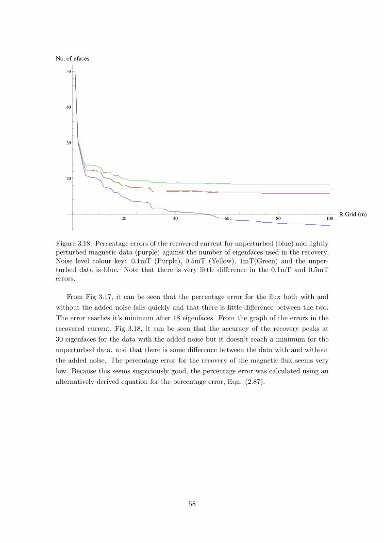
20 40 60 80 100R Grid HmL

20

30

40

50

No. of efaces

Figure 3.18: Percentage errors of the recovered current for unperturbed (blue) and lightlyperturbed magnetic data (purple) against the number of eigenfaces used in the recovery.Noise level colour key: 0.1mT (Purple), 0.5mT (Yellow), 1mT(Green) and the unper-turbed data is blue. Note that there is very little di↵erence in the 0.1mT and 0.5mTerrors.

From Fig 3.17, it can be seen that the percentage error for the flux both with and

without the added noise falls quickly and that there is little di↵erence between the two.

The error reaches it’s minimum after 18 eigenfaces. From the graph of the errors in the

recovered current, Fig 3.18, it can be seen that the accuracy of the recovery peaks at

30 eigenfaces for the data with the added noise but it doesn’t reach a minimum for the

unperturbed data. and that there is some di↵erence between the data with and without

the added noise. The percentage error for the recovery of the magnetic flux seems very

low. Because this seems suspiciously good, the percentage error was calculated using an

alternatively derived equation for the percentage error, Eqn. (2.87).

58

20 40 60 80 100R Grid HmL

5

10

15

20

25

Percentage error

Figure 3.19: Percentage errors of the recovered flux against the number of eigenfaces usedin the recovery using the second equation for the percentage error. Noise level colour key:0.1mT (Purple), 0.5mT (Yellow), 1mT(Green) and the unperturbed data is blue. Notethat there is very little di↵erence in the 0.1mT and unperturbed errors.

As can be seen in Fig 3.19, using a second method to calculate the percentage error

yields the same results as the first method. After further reflection, it was finally realized

that this result is due to the fact that the percentage error calculated is a percentage

error for the entire flux grid and the low percentage error is helped by the majority of

gridpoints which are outside the plasma. The “vacuum flux” (i.e. the flux outside the

plasma) is accurately determinable from magnetic measurements and combining these

with those inside the plasma, which have a higher error, leads to the overall 1% result.

To show this, a graph of the percentage error as a function of major radius, R, along the

horizontal line at fixed Z = Zmagnetic axis

was made for the three noise levels of 0.1mT,

0.5mT and 1mT.

59

1.5 2.0 2.5R Grid HmL

2

4

6

8

Percentage error

Figure 3.20: Percentage errors of the recovered flux as a function of the major radius Rwith the Z values fixed at the magnetic axis. Noise level colour key: 0.1mT (blue), 0.5mT(Purple) and 1mT(Gold)

As can be seen from Figure 3.20, the percentage error is low (< 1% for 0.1mT of added

noise and < 3% for 1mT of added noise) outside the plasma and increases to 7/9% for

0.1mT/1mT of added noise at the center of the plasma. The errors outside the plasma

in Figure 3.18 are similar to the errors obtained in figures 3.15 and 3.17 showing that

the low error outside the plasma is a↵ecting the errors in recovering the magnetic flux.

The percentage error as a function of R was also calculated for the current density and is

shown in Figure 3.21.

60

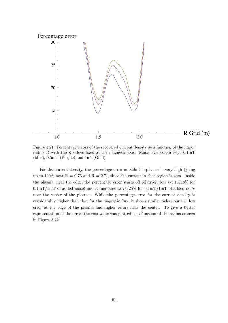
1.0 1.5 2.0R Grid HmL

15

20

25

30Percentage error

Figure 3.21: Percentage errors of the recovered current density as a function of the majorradius R with the Z values fixed at the magnetic axis. Noise level colour key: 0.1mT(blue), 0.5mT (Purple) and 1mT(Gold)

For the current density, the percentage error outside the plasma is very high (going

up to 100% near R = 0.75 and R = 2.7), since the current in that region is zero. Inside

the plasma, near the edge, the percentage error starts o↵ relatively low (< 15/18% for

0.1mT/1mT of added noise) and it increases to 23/25% for 0.1mT/1mT of added noise

near the center of the plasma. While the percentage error for the current density is

considerably higher than that for the magnetic flux, it shows similar behaviour i.e. low

error at the edge of the plasma and higher errors near the center. To give a better

representation of the error, the rms value was plotted as a function of the radius as seen

in Figure 3.22

61

1.5 2.0 2.5R Grid HmL

0.2

0.4

0.6

0.8

1.0

1.2

1.4

rmse HMAêm^2L

Figure 3.22: rms value of the recovered current as a function of the major radius R withthe Z values fixed at the magnetic axis. Noise level colour key: 0.1mT (blue), 0.5mT(Purple) and 1mT(Gold)

In Figure 3.22, it can be seen that the rms value peaks near the center of the plasma

and decreases furthur away from the center. This is of a similar form to Figure 3.20. It can

also be seen that the rms value is decreasing yet non-zero outside the plasma (especially

in the range 1 <R< 1.5), explaining the rapidly increasing percentage errors outside the

plasma in Figure 3.20.

Figures 3.17 - 3.22 were generated in the notebook regfp.nb using Eqn. (2.90). To

generate figures 3.17 - 3.20, the percentage error was calculated as the number of eigenfaces

used to recover the flux or current. To calculate the percentage errors as a function of the

major radius, the values of the flux or current were taken along the magnetic axis and

calculated the percentage error using these.

62

Chapter 4

Conclusion

The aim of this thesis was the development of a Mathematica code that uses statistical

methods to generate a compact representation of 2D tokamak equilibrium flux and current

density function. The statistical basis for the work was described in Chapter 2 and the

results from the code applied to some data from the ASDEX Upgrade tokamak were

shown in Chapter 3.

Using Function Parameterization in conjunction with singular value decomposition

was successful since this drastically reduced the size of the data sets that were being used.

A set of 2546 129⇥257 grid datasets (as a 2546⇥33153 matrix) was reduced to a 2546⇥2546

matrix in which a majority of the information was held in a few eigenvectors.This was

then used in a once o↵ calculation of the Fourier moments from which the dataset can

be recovered in conjunction with the eigenvectors. These Fourier moments were then

regressed so that they could be recovered from diagnostic data from the tokamak and

the magnetic flux and current density profiles can be recovered from these. The methods

described in this thesis proved to be quick and reliable methods to recover magnetic

parameters from magnetic data. The magnetic flux/ current can be recovered from the

magnetic data, pre-calculated regression coe�cients and the corresponding eigenfaces in

seconds on a 2.0GHz, 6 Gb Dell XPS laptop. However, the eigenfaces require a few

minutes to calculate although this calculation is necessary only once. While ASDEX

Upgrade uses conventional processors which are comparable to the laptop used, programs

run for it will be in Fortran or C which are faster than Mathematica since it is an

interpreted language. One possibility for improvement is to remove the area outside the

plasma from the recovered current database so that the recovery errors can be better

determined.

63

Appendix A

Table of notations

This gives a list of some notations used along with the page they first appear on.

J—The current density (Amperes per square meter) . . . . . . . . . . . . . . . . . . . . . . 7

B—The magnetic field (Tesla) . . . . . . . . . . . . . . . . . . . . . . . . . . . . . . . . . . . . . . . . . . . . 7

E—The electric field (Newtons per Coulomb) . . . . . . . . . . . . . . . . . . . . . . . . . . . . . 7

D—The electric displacement field (Coulbombs per square meter) . . . . . . . . . 7

x(n⇥ 1)—A column vector of measurements consisting of the value of a variable X

for n randomly selected states . . . . . . . . . . . . . . . . . . . . . . . . . . . . . . . . . . . . . . . . . .23

xi

—The sample mean of the ith variable . . . . . . . . . . . . . . . . . . . . . . . . . . . . . . . . . 23

S—The covariance matrix . . . . . . . . . . . . . . . . . . . . . . . . . . . . . . . . . . . . . . . . . . . . . . . 24

�—The matrix of principal components . . . . . . . . . . . . . . . . . . . . . . . . . . . . . . . . . 27

SV D —Singular Value Decomposition . . . . . . . . . . . . . . . . . . . . . . . . . . . . . . . . . . . . . . . 24

U—The left handed singular vectors of a matrix . . . . . . . . . . . . . . . . . . . . . . . . . 25

V—The right handed singular vectors of a matrix . . . . . . . . . . . . . . . . . . . . . . . .25

Fj

—A set of eigenfaces . . . . . . . . . . . . . . . . . . . . . . . . . . . . . . . . . . . . . . . . . . . . . . . . . . . 25

'—The fourier-like amplitudes . . . . . . . . . . . . . . . . . . . . . . . . . . . . . . . . . . . . . . . . . . 25

64

rmsv —The root mean squared value . . . . . . . . . . . . . . . . . . . . . . . . . . . . . . . . . . . . . . . . 34

rmse—The root mean squared error . . . . . . . . . . . . . . . . . . . . . . . . . . . . . . . . . . . . . . . . 34

65

Appendix B

References

[1]: P.J. Mc Carthy, PhD thesis, University College Cork, 1992.

[2]: Chen, F.F.,“’Introduction to Plasma Physics and Controlled Fusion”, Plenum Press,

New York, 1974

[3]: Robert J. Goldston and Paul H. Rutherford., “Introduction to plasma physics”,

Institute of Physics Pub., c1995.

[4]: Gurnett, Donald A,“’Introduction to Plasma Physics”, Cambridge University Press,

2005

[5]: Bellan,Paul Murray,“Fundamentals of Plasma Physics”, Cambridge University Press,

2006

[6]: Wesson, J., “Tokamaks”, Clarendon Press, Oxford 1987

[7]: W. Treuterrer, J. Gernhardt, O. Gruber, P. Mc Carthy, G. Raupp, U. Seidel, ASDEX

Upgrade Team, “Plasma Shape Control Design in ASDEX Upgrade”, Fusion Technol-

ogy: Proceedings of the 19th Symposium on Fusion Technology, Lisbon, Portugal, 16-20

September 1996: C. Varandas, F. Serra (Editors) (1997) 933-936

[8]: Y. Sadeghi, G. Ramogida et al, “Real-Time Reconstruction of Plasma Equilibrium

in FTU” , IEEE Transactions on Plasma Science, Vol. 38 (2010) 352.

[9]: L. Giannone, W. Schneider, PJ MC Carthy et al, “Real time magnetic field and

flux measurements for tokamak control using a multi-core PCI Express system”, Fusion

Engineering and Design, Vol. 84 (2009) 825.

[10]: LL Lao, HE St.John et al., “MHD equilibrium reconstruction in the DIII-D toka-

mak”, Fusion Science and Technology Vol. 48 (2005) 968.

[11]: W. Zwingmann, “Equilibrium analysis of steady state tokamak discharges”, Nucl.

Fusion Vol. 43 (2003) 842.

[12]: LC Appel, MK Bevir, MJ Walsh, “Equilibrium reconstruction in the START toka-

mak”, Nucl. Fusion Vol. 41 (2001) 169.

[13]: HP Callaghan, PJ MC Carthy, J Geiger, “Fast equilibrium interpretation on the

W7-AS stellarator using Function Parameterization”, Nucl. Fusion, Vol. 39 (1999) 509

[14]: JR Ferron, ML Walker et al., “Real time equilibrium reconstruction for tokamak

discharge control”, Nucl. Fusiion Vol. 38 (1988) 1055

66

[15]: M. Turk and A. Pentland, J. Cognitive Neuroscience 3 (1991) 71-86.

[16]: DY Tsao, MS Livingstone, “Mechanisms of face perception”, Annual review of

Neuroscience, vol. 31, (2008) pp. 411-437

[17]: R. Ebrahimpour, E. Kabire, H. Esteky, MR Yousefi, “View-independent face recog-

nition with mixture of experts”, Neurocomputing, vol. 71 (2008) pp. 1103-1107.

[18]: S. Ullman, “Object recognition and segmentation by a fragment-based hierarchy”,

Trends in cognitive sciences, Vol. 11 (2007) pp. 58-64

[19]: PF Felzenszwalb, DP Huttenlocher, “Pictorial structures for object recognition”,

International journal of computer vision, vol. 61 (2005) pp 55-79

[20]: C. Fredembach, M. Schroder, S. Susstrunk, “Eigenregions for image classification”,

IEEE transactions on pattern analysis and machine intelligence, Vol. 26 (2004) pp. 1645-

1649

[21]: MJ Lyons, J. Budynek, S. Akamatsu, “Automatic classification of single facial im-

ages”, IEEE transactions on pattern analysis and machine intelligence , Vol. 21 (1999)

pp. 1357-1362

[22]: S. Lawrence, CL Giles, AC Tsoi, AD Back, “Face recognition: A convolutional

neural-network approach”, IEEE transactions on neural networks, Vol. 8 (1997) pp. 98-

113

[23]: Searle, “Matrix Algebra Useful for statistics”, New York, Wiley, 1982

[24]: Teukolsky, Vetterling, Flannery, “Numerical Recipies in Fortran, Second Edition”,

Cambridge University Press, 1992

[25]: P.J. Mc Carthy, S. OMahony and the ASDEX Upgrade Team, “Eigenface repre-

sentation of equilibrium flux using Function Parameterization” (38th EPS Conference on

Controlled Fusion and Plasma Physics, Strasbourg, 27th June 1st July 2011) Europhysics

Conference Abstracts 38 (2011) P2.092.

[26]: Mardia, K.V., Kent, J.T., Bibby, J.M, “Multivariate Analysis”, Academic Press,

London, 1979

[27]: J.D. Huba, Naval Research Laboratory (NRL) Plasma Formulary,

http://wwwppd.nrl.navy.mil/

[28]: PJ Mc Carthy, CB Forest, M Foley, L Giannone, O Gruber, J Hobirk, LD Hor-

ton, K Lackner, P Martin, M Reich, W Schneider, ACC Sips and ASDEX Ugrade Team,

“ Plasma geometry and current profile identification on ASDEX Upgrade using an in-

tegrated equilibrium generation and interpretation system”. 21st IAEA Fusion Energy

Conference, Chengdu , China 16th-21st October 2006 TH/P3-7.

[29]: K. Lackner, “Computation of ideal MHD equilibria”, Comp. Phys. Commun. Vol.

12 (1976) 33-44.

67

Appendix C

Mathematica Code

During this project, code was written by the student that performs singular value de-

composition and calculates eigenfaces and uses the results of these to recover magnetic

flux and current. The results presented in this thesis were mainly calculated using two

notebooks (a file written using Mathematica) : SVD.nb and regfp.np. SVD.nb performs

singular value decomposition on the training database of either the magnetic flux or the

magnetic current. It outputs the eigenfaces and Fourier components corresponding to the

given training database.

regfp.np performs a Function Parameterization on the Fourier moments calculated in

SVD.np with the principal components of the magnetic measurements. It then recovers

the magnetic flux or the current using the techniques described in the thesis and compares

the accuracy of the recovered data compared to the training database.

The notebook cplot.nb is also included in the appendix as it was used to generate

the contour plots of the training databases and the eigenfaces. This was written by the

student based o↵ code by Dr. Patrick McCarthy.

68

Parsimonious reconstruction of 2D MHD equilibrium states...

Documents

Transcript of Parsimonious reconstruction of 2D MHD equilibrium states...