A Model for High-Strain-Rate

Deformation of Uranium-Niobium Alloys

LA-14034-MSApproved for public release;

distribution is unlimited.

This report was prepared as an account of work sponsored by an agency of the United StatesGovernment. Neither the Regents of the University of California, the United States Government norany agency thereof, nor any of their employees make any warranty, express or implied, or assumeany legal liability or responsibility for the accuracy, completeness, or usefulness of any information,apparatus, product, or process disclosed, or represent that its use would not infringe privately ownedrights. Reference herein to any specific commercial product, process, or service by trade name,trademark, manufacturer, or otherwise does not necessarily constitute or imply its endorsement,recommendation, or favoring by the Regents of the University of California, the United StatesGovernment, or any agency thereof. The views and opinions of authors expressed herein do notnecessarily state or reflect those of the Regents of the University of California, the United StatesGovernment, or any agency thereof. Los Alamos National Laboratory strongly supports academicfreedom and a researcher's right to publish; as an institution, however, the Laboratory does notendorse the viewpoint of a publication or guarantee its technical correctness.

Los Alamos National Laboratory, an affirmative action/equal opportunity employer, is operated by theUniversity of California for the United States Department of Energy under contract W-7405-ENG-36.

A Model for High-Strain-Rate Deformation of

Uranium-Niobium Alloys

F.L. Addessio

Q.H. Zuo

T.A. Mason

L.C. Brinson

LA-14034-MSIssued: May 2003

v

Contents

Abstract .......................................................................................................... 1

I. Introduction .............................................................................................. 1

II. Thermodynamic Framework.......................................................................... 4

III. Constitutive Model ..................................................................................... 9A. Equation of State ............................................................................... 9B. Reorientation.................................................................................... 11C. Transformation ................................................................................. 12D. Rate-Dependent Plasticity and Ductile Failure ........................................... 12E. Phase Diagram.................................................................................. 14

IV. Numerical Implementation ............................................................................ 15A. Reorientation.................................................................................... 16B. Plasticity ......................................................................................... 16C. Transformation ................................................................................. 17D. Plasticity and Transformation................................................................ 18

V. Results .................................................................................................... 19

VI. Summary ................................................................................................. 28

Acknowledgements ............................................................................................ 29

References....................................................................................................... 29

Figures

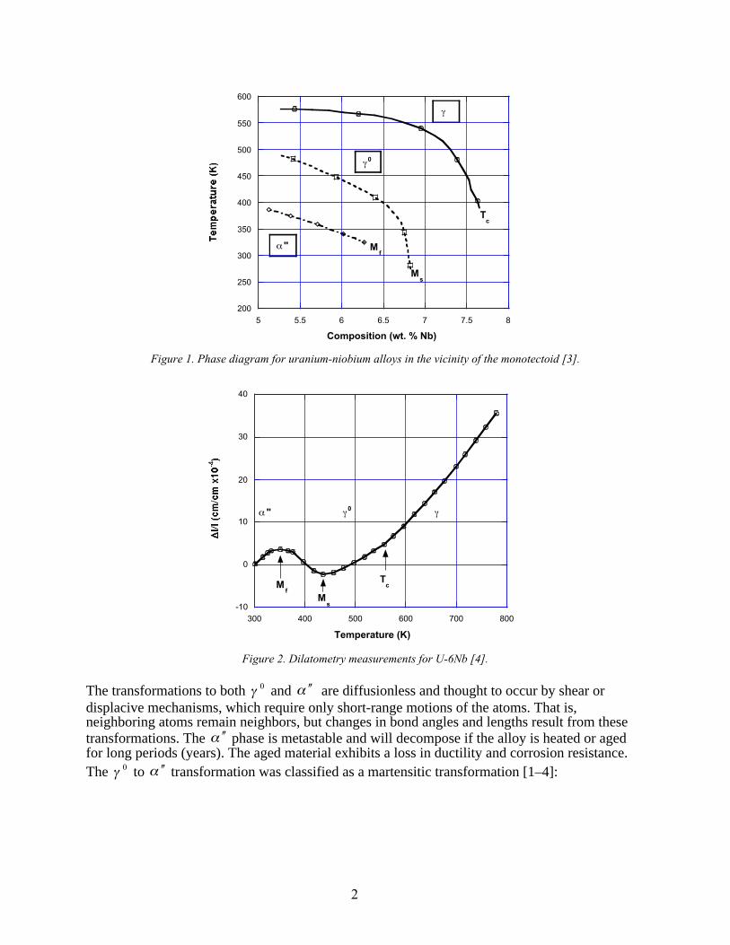
Figure 1. Phase diagram for uranium-niobium alloys in the vicinity of the monotectoid [3]. .. 2

Figure 2. Dilatometry measurements for U-6Nb [4]. ................................................... 2

Figure 3. Phase diagram for a representative shape-memory alloy. ................................. 14

Figure 4. Phase diagram used for U-6Nb studies. ....................................................... 15

Figure 5. Representative mechanical response using the material model. .......................... 22

Figure 6. Comparison of simulations and data [3] for stress and temperature paths versusstrain for U-6Nb. .................................................................................. 23

Figure 7. Comparison of simulations and data for uniaxial stress esperiments [5]. ............... 25

Figure 8. Comparison of simulations and data for plate impact experiments [49]. ............... 26

Figure 9. Schematic diagram of the plate impact experiments [49]. ................................. 27

Tables

Table I. Material parameters (yield strength for the material of Vandermeer [1–4] isprovided in parentheses). ........................................................................ 20

Table II. Material parameters for crystal reorientation (properties for the material ofVandermeer [1–4] are provided in parentheses). ............................................ 21

Table III. Plate impact experiments ........................................................................ 27

vi

1

A Model for High-Strain-Rate Deformations of Uranium-Niobium Alloys

F.L. Addessio*, Q.H. Zuo, T.A. MasonTheoretical Division

Los Alamos National LaboratoryLos Alamos, NM 87545(*addessio@lanl.gov)

L.C. BrinsonDepartment of Mechanical Engineering

Northwestern UniversityEvanston, IL 60208

Abstract

A thermodynamic approach is used to develop a framework for modeling uranium-niobium alloys under the conditions of high strain rate. Using this framework, a three-dimensional phenomenological model, which includes nonlinear elasticity (equation ofstate), phase transformation, crystal reorientation, rate-dependent plasticity, andporosity growth is presented. An implicit numerical technique is used to solve theevolution equations for the material state. Comparisons are made between the modeland data for low-strain-rate loading and unloading as well as for heating and coolingexperiments. Comparisons of the model and data also are made for low- and high-strain-rate uniaxial stress and uniaxial strain experiments. A uranium-6 weight percentniobium alloy is used in the comparisons of model and experiment.

I. Introduction

In an effort to improve ductility and corrosion resistance, niobium has been used to alloyuranium. Uranium-niobium (U-Nb) alloys within the range from 5 weight percent (U-5Nb) to 8weight percent (U-8Nb) of niobium exhibit the shape memory effect [1–5]. A phase diagram forU-Nb alloys in the vicinity of the monotectoid composition (U-6Nb) is provided in Fig. 1. Atelevated temperatures (T > 600 K), U-6Nb is stable in the body-centered cubic (bcc) γ phase. Asthe alloy is cooled rapidly to room temperature, it undergoes a two-stage transformation process.Dilatometry measurements (Fig. 2) indicate that at Tc ~ 570 K, a displacement-orderingtransformation from the γ phase to a distorted bcc (tetragonal) 0γ phase is observed. The γ to

0γ transformation temperature was denoted Tc to indicate the constriction arrest, which is theaccepted notation for ordering reactions. Because this transformation is a rapid, isothermaltransformation at high temperature, an in-situ structural investigation is difficult to obtain.Information can be obtained for this transformation at larger niobium concentrations, where the

0γ phase exists at room temperature (Fig. 1). This transformation was considered to be a pre-

martensitic phenomenon. As U-6Nb is cooled further, the transformation from the 0γ phase tothe monoclinic α ′′ phase is observed. This transformation starts at the temperature Ms ~ 435 Kand is finished by Mf ~ 350 K.

2

200

250

300

350

400

450

500

550

600

5 5.5 6 6.5 7 7.5 8

Composition (wt. % Nb)

α" Mf

Ms

Tc

γ

γ0

Figure 1. Phase diagram for uranium-niobium alloys in the vicinity of the monotectoid [3].

-10

0

10

20

30

40

300 400 500 600 700 800

Temperature (K)

α " γ0 γ

Tc

Ms

Mf

Figure 2. Dilatometry measurements for U-6Nb [4].

The transformations to both 0γ and α ′′ are diffusionless and thought to occur by shear ordisplacive mechanisms, which require only short-range motions of the atoms. That is,neighboring atoms remain neighbors, but changes in bond angles and lengths result from thesetransformations. The α ′′ phase is metastable and will decompose if the alloy is heated or agedfor long periods (years). The aged material exhibits a loss in ductility and corrosion resistance.The 0γ to α ′′ transformation was classified as a martensitic transformation [1–4]:

3

1. the α ′′ microstructure is similar to nonferrous alloys that undergo a martensitictransformation as determined by diffraction techniques,

2. the volume expansion accompanying the transformation is small,3. the stress versus strain behavior under uniaxial tension exhibits reorientation of the

crystal structure, and4. the alloy displays strain recovery on heating.

The time for the 0γ to α ′′ transformation is short (approximately 10 ns). The martensitestart (Ms) and finish (Mf) temperatures are inverse functions of the heating rate. The dependenceof Ms and Mf on the heating rate decreases for higher rates. The thermal transformationhysteresis associated with the reverse transformation was considered negligible to withinexperimental error [1,2]. However, recent experiments have better defined the differencebetween the austenite ( 0γ ) finish (Af) and martensite (α ′′ ) start (Ms) as well as the austenite start(As) and martensite finish (Mf) temperatures.

At room temperature, the monoclinic α ′′ lattice appears as martensite plates, which canform in many orientations (variants) in the same parent phase (γ ) grains. These variantssubdivide the parent grains. The initial crystalline structure is random. Consequently, materialtexture can be neglected. Furthermore, little difference was observed between the tensile andcompressive responses of the material [5]. An elastic material response is observed below strainsof approximately 0.3%. As the α ′′ phase is loaded beyond strains of 0.3%, the deformationprocess is dominated by continuous crystalline reorientation associated with a detwinningprocess, as reported by x-ray and neutron diffraction experiments [6,7]. That is, orientations(variants) that are favored by the loading direction increase in volume fraction at the expense ofless favored orientations. This reorientation process is observed for large strains (εL ~ 7%). Oncethe strain limit (εL) for the reorientation process is exceeded, dislocation slip is observed todominate. For strains between 0.3% and 7%, moderate strain recovery is obtained during anonlinear unloading process. The yield strength varies little with niobium content for alloys closeto the monotectoid composition. Experimental data [5] indicate a minimum yield strength foralloys of 6 weight percent. Heat activated strain recovery (εR ~ 4.2%), which is associated withmartensite recovery, can be obtained.

Many applications utilizing shape memory alloys (SMAs) require large deformationsunder high-strain-rate conditions with few mechanical or thermal cycles. Applications include,for example, impact, penetration, and weapons performance scenarios. In addition to phasetransitions and reorientation, physical processes including nonlinear elasticity, plastic slip, andfailure must be modeled to address large-strain, high-strain-rate deformations. Nonlinearelasticity is necessary to model the material response to shock loading accurately. At highstresses, dislocations are generated within the material, resulting in irreversible strains.Deforming the detwinned state plastically also can inhibit the material from transforming back tothe parent state when the temperature of the material is increased. The preferred variantmicrostructure is ‘locked in’ by the dislocations, preventing the material from transforming backto the parent or multiple variant microstructure. Subjecting the material to higher stressesultimately leads to pore nucleation, growth, and coalescence, which result in ductile failure.

4

Theories that address the phase transition and reorientation phenomena inherent in SMAsare available for a number of length scales. At the atomistic scale, molecular dynamicsimulations have been conducted, which have provided insight into phase transitions [8]. Theatomistic models may be used to guide the free-energy formulations used in single-crystalmodels. On the scale of a single crystal, Ginzburg-Landau [9] and Multi-variant [10–12]theories, which model the phase transition and reorientation processes due to changes in thestress and temperature, are available. Homogenization techniques [13] can be used to obtain thepolycrystalline response using the single-crystal theories. The polycrystal theories may be usedto develop mechanical potentials, which are necessary for engineering models. Finally,macromechanical models can be implemented into computer analyses to obtain the response ofengineering structures utilizing SMAs to mechanical and thermal changes. A number ofmacromechanical models are available in the literature [14–18]. The majority of themacromechanical models address one-dimensional problems under the conditions of smallstrains and small strain rates. Models, which address large-strain conditions, including plasticity[19] also have been developed.

A phenomenological approach is provided for modeling high-strain-rate deformations,including nonlinear elasticity, reorientation (twinning), dislocation slip (plasticity), solid-solidphase transitions, and material failure. A framework for the constitutive model will be pursued inSection II, using a thermodynamic approach for modeling SMAs. In Section III, the frameworkwill be generalized to address high-strain-rate applications. An implicit numerical approach forimplementing the constitutive model into finite-element or finite-difference structural analyseswill be considered in Section IV. Simulations utilizing the model and comparisons to data will bepresented in Section V. A summary will be provided in Section VI.

II. Thermodynamic Framework

The total specific Helmholtz free energy )(χψ , where ],,,,,,[ ξεεεεχ iij

rpeij DT= are the

state variables, is expressed as the average of the free energy [20–26] of each speciesAMkDT rpe

ijk ,),,,,,( =εεεψ and the free energy [26] of mixing ),( ξεψ i

ijmix

ψ χ ξψ ξ ψ ψ( ) ( ) = + − +M A mix1 . (II.1)

The variables ,, iij

eij εε T, and ξ are the elastic strain, inelastic strain, temperature, and volume

fraction of the product phase (M), respectively. Also, pε and rε are hardening variables forplasticity and crystal reorientation. The variable D characterizes the amount of material damage.The Helmholtz free energy for the product and parent (A) phases may be written [20,21,26]

ψ ε ε ερ

λ ε ε µ ε ερβ ε θ θ

γ ε η ε θ ψ

kije p r k

kke

mme k

ije

ije k

kke

k

k p p k r r k k

T Dc

T

f D f s k M A

( , , , , ) [ ]

( , ) ; ,

= + − −

+ + ( )− + =

12

21

2 0

2

0 0

. (II.2)

5

It is assumed that the material of interest is isotropic. In Eq. II.2, kλ and kµ are the Lame

coefficients, kkk Bαβ 3= where kα is the coefficient of thermal expansion and kB is the bulk

modulus ( kkkB µλ 32+= ), ck is the specific heat, and θ is a temperature difference ( 0TT −=θ ).

The reference temperature is 0T . The parameters kγ and kη are material parameters related toplasticity and reorientation, respectively. Also, ρ is the material density, which is assumed to be

identical for both phases. The function ),( Df pp ε is a general isotropic description for plasticity[20]. It is assumed that the material fails in a ductile fashion. Consequently, both strain hardening( pε ) and softening due to damage (D) are included in the expression for plasticity [27–29]. Thefunction )( rrf ε is an isotropic description for crystal reorientation, which is written in terms of

the hardening parameter rε . The parameters ks0 and k0ψ are material constants, which define the

reference state. The free energy of mixing is expressed as a quadratic function of the volumefraction of the phases and the inelastic strain [26]

ξεεεξξεψ iijij

ikl

iijijkl

iij

mix bbb ),( 212

21 ++= . (II.3)

The coefficients ,, ijbb and ijklb are material parameters. The rate of deformation (strain rate) isdecomposed into its elastic and inelastic components [26]

iij

eijij εεε &&& += . (II.4)

The inelastic rate of deformation (iijε& ) includes the rates due to crystal reorientation (

rijε& ), phase

transformation (tijε& ), and slip plasticity (

pijε& ). Furthermore, it is assumed that the rate of

deformation due to transformation may be expressed as [26, 30–33]

ξε && ijtij Λ= (II.5)

where [26]

<+

≥+=Λ

0:

0:

031

0

031

023

ξδ

ξδτ

&

&

ijt

tij

ijij

ij

ge

eh

gs

h . (II.6)

In Eq. II.6, ijs is the deviatoric component of the stress )( 3

1ijkkijijs δσσ −= , τ is the von Mises

stress )( 23

ijij ss=τ , and te is the effective transformation strain )( 32 t

ijtij

t eee &&& = . The deviatoric

component of strain is ije . Also, 0h and 0g are material constants, where 0h is the recovery

strain and 0g is the relative volume change due to transformation.

6

The generalized thermodynamic forces may be derived using Eqs. II.1–II.3 [20–22]

sT

c

Tskk

e

ijije kk

eij ij

eij

= − = + +

= = + −

∂ψ∂

βρε θ

σ ρ∂ψ∂ε

λε δ µε βθδ

00

2

Ω

Ω

Ω

dp p

pp

p p

p

rr

r r

r

iji

iji ijkl kl

iij

D

f D

D

f D

f

b b

( , )

( , )

( )

( )

= =∂

∂

= =∂

∂

= =∂∂

= = +

=

ρ∂ψ∂

ργε

ρ∂ψ∂ε

ργεε

ρ∂ψ∂ε

ρηεε

µ ρ∂ψ∂ε

ρ ε ξ

µ ρ∂ψ∂ξ

ξ

( )

,

= + − −

+ ( ) + ( ) − + + +[ ]

12

0

2

0 0

22

∆ ∆ ∆∆

∆ ∆ ∆ ∆

λε ε µε ε βε θρ

θ

ρ γ ε η ε θ ψ ξ ε

kke

mme

ije

ije

kke

p p r rij ij

i

c

T

f D f s b b

. (II.7)

In Eq II.7, s and ijσ are the entropy and Cauchy stress, respectively. Average material properties

( ηγβµλ ,,,,,, 0sc ) are defined using the rule of mixtures, e.g.

AM λξξλλ )1( −+= . (II.8)

Also, AM λλλ −=∆ denotes the difference in the material properties of the product and parentphases.

Consider the Clausius-Duhem inequality [20–23], which defines the dissipation rate (Φd)for the thermomechanical process in the absence of external heat sources

0 ) ( , ≥−+−=ΦT

TqTs ii

ijijd&&& ψρεσ , (II.9)

where iq is the heat flux. Substituting Eqs. II.4, II.5, and II.7 into Eq. II.9 results in theexpression for the dissipation rate

Φ Σ Ω Π Σ Ω Ωd ij ijr r r

ij ijp d p p i iD

q T

T ˙ ˙ ˙ ( ˙ ˙ ˙ ) ,= −( ) + + − − − ≥ε ε ξ ε ε 0 . (II.10)

The thermodynamic variables Σij and Π are defined as [26]

7

ξµ

µσ

−ΛΣ=Π

−=Σ

ijij

iijijij

. (II.11)

It is assumed that the dissipation may be decomposed [20] into four separate andindependent processes, three mechanical (reorientation, phase transformation, and combined slipplasticity and damage) and one thermal. Therefore, three independent mechanical potentials forreorientation, transformation, and plasticity ( ,, tr φφ and pφ ) will be defined, from which theinelastic parameters may be obtained [20,21,24]

˙ ( , )

˙

˙( , )

˙

˙ ( )

˙

˙ ( , , )

˙

˙( , , )

˙

˙

ε∂φ

∂λ

ε∂φ

∂λ

ξ∂φ∂

λ

ε∂φ

∂λ

ε∂φ

∂λ

ijr

rij

r

ij

r

rr

ijr

rr

tt

ijp

pij

d p

ij

p

pp

ijd p

pp

D

=

=−

=

=

=−

Σ Ω

Σ

Σ Ω

ΩΠΠ

Σ Ω Ω

Σ

Σ Ω Ω

Ω

( , , )

˙= −∂φ

∂λ

pij

d p

dpΣ Ω Ω

Ω

. (II.12)

In Eqs. II.12, rλ& , tλ& , and pλ& are the Lagrange multipliers for crystal reorientation,transformation, and plasticity, respectively. The thermal potential results in Fourier’s Law forheat conduction [20]. Consider, for example, the inelastic mechanical potentials

φ ε

φ

φ

r

ij ijr r r

t t

pij ij

p d p

Y

Y

( )

( , , )

= ′ ′ − +[ ] =

= =

= ′ ′ − =

32 0

32

0

0

0

Σ Σ Ω Ω

Π

Σ Σ Ω Ω Σ

m . (II.13)

In Eq. II.13, ijijij δΣ+Σ=Σ′ and kkΣ−=Σ 3

1 are the deviatoric and volumetric components of

ijΣ , respectively. The two signs (+/-) in Eq. II.13b allow for hysteresis [26] in the phasetransformation process. The inelastic variables may be obtained from Eqs. II.12 and II.13.Therefore, for crystal reorientation and transformation, the inelastic variables are

t

rr

rijrij

λξ

λε

λε

&&

&&

&&

=

=Σ′

Σ′=

2

3

. (II.14)

8

The multipliers for reorientation ( rλ& ) and transformation ( tλ& ) are obtained from the consistency

conditions ( 0=rφ& and 0=tφ& ). In Eq. II.14, Σ′ is an effective stress ( ijijΣ′Σ′=Σ′ 23 ) .

Assume, for example, that the plastic term in the expression for the Helmholtz freeenergy (Eq. II.2) may be written

)1ln()(),( 0 DgDf ppp −Σ

= ερ

ε . (II.15)

Also, if the plastic-yield function degrades linearly with the hydrostatic stress (Σ < 0) andlinearly with damage, then

Y D hg hp d p p p

p

dp p( , , ) ( )

( ) ( )( )Ω Ω Σ Σ Ω Ω

Σ ΣΩ

Ω Ω= − ( ) −[ ] =− −1 00

0

γ ε . (II.16)

Substituting Eqs. II.15 and II.16 into II.12 provides the plastic-strain rate ( pijε& ), the strain-rate-

hardening variable ( pε& ), and the rate of change of damage (D& ):

˙ ˙

˙ ( ) ( ) ˙

˙ ( )( )

( ) ˙

ε δ λ

ε λ

γ εε

ijp ij

p

ijp

p p

p kkp

Y

D h

D Dh

g h

=′

′+

∂∂

= −

= −( ) ′

3

213

1

10

Σ

Σ Σ

Σ

Σ

Σ Σ

. (II.17)

Eq. II.17c resembles a classical void growth expression [27] if the damage (D) is interpreted asthe void volume fraction (φ ). The advantage of this associative formulation is that the Clausius-Duhem inequality is satisfied automatically. That is, with a judicious choice for the inelasticmechanical potentials in terms of the generalized thermodynamic forces, an associatedformulation can be obtained systematically for the state variables ( Dpp

ijrr

ij ,,,,, εεξεε ), whichautomatically satisfy the dissipation inequality.

9

III. Constitutive Model

In an effort to address high-strain-rate applications, the framework developed in SectionII will be generalized in a heuristic fashion. Extensions include nonlinear elasticity (equation ofstate), rate-dependent plasticity, and ductile failure by porosity growth. Phenomenologicalmechanical potentials for crystal reorientation, phase transformation, and plasticity will beintroduced for demonstrative purposes. Physically based potentials will be pursued in a futureinvestigation. Finally, a phase diagram will be introduced as a method of summarizing the modelin a two-dimensional (stress versus temperature) space.

A. Equation of State

From Eq. II.7b, the stress is written as

ijeijij

ekkij βθδµεδλεσ 2 −+= . (III.1)

The expression for the stress (Eq. III.1) will be generalized in this section to include high-pressure effects. The stress ( ijσ ) is decomposed into its deviatoric ( ijs ) and volumetric

( kkP σ31−= ) components

ijijij Ps δσ −= . (III.2)

The deviatoric component is written directly from Eq. III.1

eijij es 2 µ= . (III.3)

For most metals, it is a good assumption to include the effects of nonlinear elasticity only in thevolumetric (pressure) component. A nonlinear expression for the pressure is referred to as theequation of state. Consider a porous material composed of the solid material and voids.Neglecting the gas pressure in the voids, the equation of state for this porous material may bewritten as [29]

),,( )1( ),,,( ξφξφ sss evPevP −= . (III.4)

In Eq. III.4, φ is the porosity or void volume fraction. The solid material properties are

subscripted (i.e., sss Pev ,, ). Also, v and e are the specific volume and the specific internal energy

of the porous material, respectively. The difference between the solid ( se ) and porous material(e) internal energies is related to the void surface energy, which is small [29]. Therefore, it willbe assumed that e ~ es. The equation of state for the solid material may be written, for example[34],

ssssssHsss ePeP )1( )1( ),,( 021 ερεξε −Γ+Γ+= . (III.5)

10

In Eq. III.5, Γs is the Gruneisen coefficient of the solid material and 0sρ is a reference density.

The density is written in terms of the volumetric strain ( 01 sss ρρε −= ). The Hugoniot pressuremay be approximated by a polynomial,

33

221 )( )( sssH aaaP εεε ++= . (III.6)

The material coefficients in Eqs. III.5 and III.6 are obtained using a rule of mixtures (Eq. II.8) toaccount for the differences in the two phases. Using Eqs. III.2 through III.4, the stress field maybe updated from the incremental expressions

φξ∂ξ

∂

∂

∂

∂

∂φ

ξµµ

µ

dPdP

dee

Pdv

v

PdP

dsdedtrds

ss

ss

ss

s

s

ijeijijij

)1(

2

−

++−=

∆+=+

. (III.7)

In Eq III.7a, the term ijr accounts for material rotation [35,36]. For example, if a Jaumann-Nollstress rate is used, then

kjikkjikij ssr ωω −= , (III.8)

where ijω is the spin tensor. An alternative approach would be to solve the constitutive model inthe unrotated reference frame [37]. Eq. III.7b may be written as

ξεαε dKddesdBdP pkkijijskk ++Γ+−= (III.9)

where PB s )1( Γ+−=α . Eq. III.9 is obtained using the equations for conservation of mass,

kkdv

dvε= , (III.10)

and conservation of energy, in the absence of heat flux and heat source terms,

ijij dvde εσ= . (III.11)

Also, the growth of damage or porosity (Eq. II.17c) is expressed in terms of the volumetricplastic strain [27]

pkkdd εφφ )1( −= . (III.12)

The bulk modulus ( sB ), the Gruneisen coefficient ( sΓ ), and the transformation coefficient ( sK )for the solid constituent are defined by the thermodynamic derivatives

11

B vP

vP v

P

v

vP

e

KP B

BP

s ss

s s

s s ss

s e

s ss

s v

ss s

ss

s

s

=−∂∂

= −

∂∂

=∂∂

=∂∂

≈

Γ

Γ

∆ξ

. (III.13)

It is assumed that the bulk material properties are degraded linearly with solidity (i.e., sBB ω=

where φω −= 1 ). Therefore, once an equation of state has been defined for the material, the bulkmodulus, Gruneisen coefficient, and transformation coefficient may be derived using Eqs. III.13.In the above development, it has been assumed that the damage (D) is equivalent to the porosity(φ ).

B. Reorientation

Consider the irreversible potential for reorientation provided by Eq. II.13,

φ εrij

rij ij

r r rs s( , ) [ ( ) ] Σ Ω Ω Ω= − + =32 0 0 , (III.14)

where the back-stress (µ iij) has been neglected (Eq. II.11a). From Eqs. II.12 and III.14,

expressions for the rate of deformation (rijε& ) and rate of hardening ( rε& ) due to reorientation, may

be obtained as

rrr

rr

rijr

ij

rrij

s

λλφ

ε

λτ

λ∂σ∂φ

ε

&&&

&&&

=Ω∂

∂−=

== 2

3

. (III.15)

The parameter rλ& may be obtained from the consistency condition ( 0 =rφ& )

1

33

−

Ω+=

r

r

ijijr

d

des

εµ

τµ

λ && . (III.16)

Eqs. III.15 and III.16 provide the expression for the reorientation strain rate and hardening oncethe function rΩ has been specified.

12

C. Transformation

Neglecting hysteresis, the transformation potential may be written (Eq. II.13)

0 =Π=tφ . (III.17)

The thermodynamic force Π (Eq. II.11) is approximated as

0000 ψρθρξρτ ∆−∆+−−≈Π sbPgh . (III.18)

This approximation for Π results in linear transformation boundaries in the τ-T and P-T planes,which are used in classical approaches for shape-memory alloys. The rate of change of themartensite volume fraction may be written (Eq. II.12)

ttt

λλ∂∂φ

ξ &&& =Π

= . (III.19)

Again the parameter tλ& may be obtained from the consistency condition ( 0=tφ& )

])( [1

00000 kksbTsPghb

εψθξρρτρ

ξ &&&&& ∆+∆−+∆+−= . (III.20)

The material constants are obtained in a τ-T plane as

∆∆∆

∆

∆ ∆

sh

T

b s M M

s M TF s

s

00

0

0 0 0

( )

( )

= −

= −

= −

ρτ

ψ

. (III.21)

In Eq. III.21, the martensitic start (Ms) and finish (Mf) temperatures are the temperatures thatdefine the beginning and end of the phase transition from the parent (A) to the product (M)phases for zero stress conditions. The slope of the transformation boundary ( Tcm ∆∆≡ /τ ) isassumed constant.

D. Rate-Dependent Plasticity and Ductile Failure

The mechanical potential for plasticity, including material hardening and softening, isexpressed as [27–29]

φε ε

φφp ij ij

sp

sp

sp

s s

Y TY p

( , ˙ , )( , ) =

[ ]− =

32

2 0 . (III.22)

There are numerous models for the plastic flow stress (Ysp). For this development, a

phenomenological model will be used [38]

13

Y T c c cT T

T Tsp

sp

sp

sp n s

p

m

m

( , ˙ , ) ( ) ln˙˙

ε ε εεε

= +[ ] +

−−−

1 2 3

0

0

0

1 1 . (III.23)

In Eq. III.23, Tm is the melting temperature of the material, and 10 1 −= sε& is a reference strain

rate. The constants ci, n, and m are material parameters. Also, psε& is the equivalent plastic-strain

rate in the solid material. The equivalent plastic-strain rate for the solid may be obtained from anexpression for the balance of plastic work [27]

ρ

εσ

ρ

ε pijij

s

ps

psY &&

= . (III.24)

In Eq. (III.24), φρρ −= 1/ s .

The degradation of the strength of the material as a result of porosity growth is written as[27–29]

( )

−−+=

0

2

23

cosh 2 1 ),(YP

qqPY φφφφ . (III.25)

In Eq. III.25, q and 0Y are material constants. Referring to Eq. II.12, the plastic-strain rate maybe written

pij

pijp

ij P

sλδ

∂∂φ

τε &&

31

2

3

−= . (III.26)

The growth of porosity (Eq. II.17c) is approximated as [27]

pkkεφφ &)1( −≈ . (III.27)

The right-hand side of the equation for the rate of change of porosity includes only the effect ofvoid growth. A more general expression also should include void nucleation and coalescence[27]. These effects will be included in a future effort.

14

E. Phase Diagram

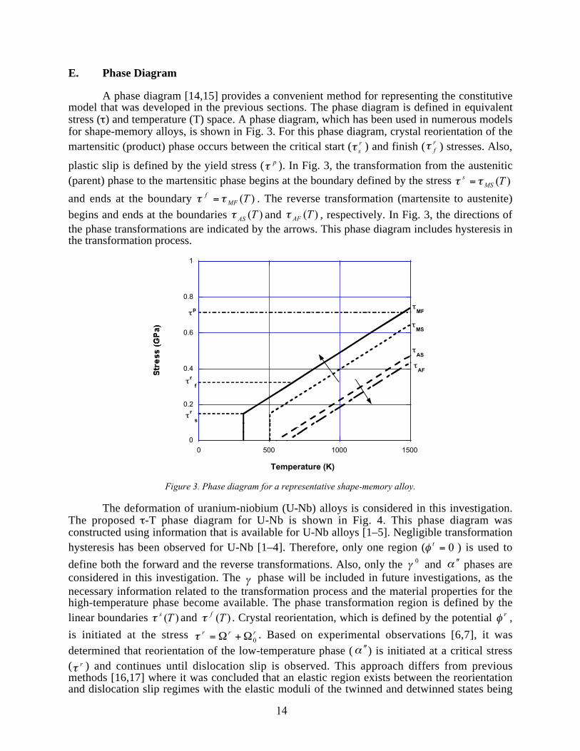
A phase diagram [14,15] provides a convenient method for representing the constitutivemodel that was developed in the previous sections. The phase diagram is defined in equivalentstress (τ) and temperature (T) space. A phase diagram, which has been used in numerous modelsfor shape-memory alloys, is shown in Fig. 3. For this phase diagram, crystal reorientation of themartensitic (product) phase occurs between the critical start ( r

sτ ) and finish ( rfτ ) stresses. Also,

plastic slip is defined by the yield stress ( pτ ). In Fig. 3, the transformation from the austenitic(parent) phase to the martensitic phase begins at the boundary defined by the stress )(TMS

s ττ =

and ends at the boundary )(TMFf ττ = . The reverse transformation (martensite to austenite)

begins and ends at the boundaries )(TASτ and )(TAFτ , respectively. In Fig. 3, the directions ofthe phase transformations are indicated by the arrows. This phase diagram includes hysteresis inthe transformation process.

0

0.2

0.4

0.6

0.8

1

0 500 1000 1500

Temperature (K)

τr s

τr f

τp

τMS

τMF

τAS

τAF

Figure 3. Phase diagram for a representative shape-memory alloy.

The deformation of uranium-niobium (U-Nb) alloys is considered in this investigation.The proposed τ-T phase diagram for U-Nb is shown in Fig. 4. This phase diagram wasconstructed using information that is available for U-Nb alloys [1–5]. Negligible transformationhysteresis has been observed for U-Nb [1–4]. Therefore, only one region ( 0=tφ ) is used to

define both the forward and the reverse transformations. Also, only the 0γ and α ′′ phases areconsidered in this investigation. The γ phase will be included in future investigations, as thenecessary information related to the transformation process and the material properties for thehigh-temperature phase become available. The phase transformation region is defined by thelinear boundaries )(Tsτ and )(Tfτ . Crystal reorientation, which is defined by the potential rφ ,

is initiated at the stress rrr0Ω+Ω=τ . Based on experimental observations [6,7], it was

determined that reorientation of the low-temperature phase (α ′′ ) is initiated at a critical stress( rτ ) and continues until dislocation slip is observed. This approach differs from previousmethods [16,17] where it was concluded that an elastic region exists between the reorientationand dislocation slip regimes with the elastic moduli of the twinned and detwinned states being

15

different. Although reorientation and plasticity occur simultaneously, they will be modeled asseparate processes in this model. Therefore, the reorientation process is assumed to end at the

start of crystal slip, which is defined by φτ YY ps

p = . This assumption is justified by theexperimental observation that below 7% strain, most of the strain may be recovered by heating.

0

0.2

0.4

0.6

0.8

1

0 500 1000 1500

Temperature (K)

τp(T)

τf(T)

τs(T)

γ0

α"

τr

Figure 4. Phase diagram used for U-6Nb studies.

IV. Numerical Implementation

For a dynamic analysis, the material state may be obtained knowing the rate ofdeformation ( ijε& ) and the temperature (T) fields, which result from solutions to the conservation

of momentum and energy equations, respectively. A robust and numerically efficient implicitnumerical algorithm [39,40] has been used to implement the proposed model. An implicitapproach offers the advantage of placing no additional stability constraints on the time-step size( tδ ) of the dynamic analysis, which utilizes the constitutive model. Consequently, compared toan explicit algorithm, larger time-step sizes may be used and hence a significant reduction in thecost of the analysis can be achieved. In this development, τs is the stress defining the start( 0=ξ ) of the phase transformation region and τf is the stress defining the end ( 1=ξ ) of the

phase transformation region for a specified temperature (T). The values of sτ and fτ areobtained from the transformation potential ( tφ ). Also, the plastic stress is defined as

φτ YY ps

p = . Similarly, the reorientation stress is rrr0Ω+Ω=τ (Fig. 4).

16

For each computational cell, a trial-material state [s*ij, P

*, φ*, ξ*] is computed first,assuming a purely elastic deformation

s s e r t

P P B s e t

ij ijn

ij ij

nkk s ij ij

n

n

* ˙

* ˙ ˙

*

*

= + −( )= − −( )=

=

2µ δ

ε δ

φ φ

ξ ξ

Γ (IV.1)

where nijs , nP , nφ , and nξ are the values of the material state at the end of the previous time

step. The trial-material state obtained from Eqs. IV.1 is used to determine where the materialstate lies on the phase diagram (Fig. 4).

A. Reorientation

If the trial-stress state satisfies the conditions τr < τ* < τp and τ* > τf, then the newmaterial state is obtained utilizing the system of equations that apply for crystal reorientation

rrr

rijrij

rijijij

s

PP

ess

0)(

2

3

*

2*

Ω+Ω=

=

=

−=

ετ

δλτ

δε

δµ

, (IV.2)

where rr δεδλ = . Also, rδλ is the incremental change in the variable rλ for the time step (i.e.,trr δλδλ &= ). Eqs. IV.2 are used to develop the following equations for the new material state

(rr

ijij Ps εε ,,, )

rrr

r

0)(

*3

1

Ω=Ω−

=

+

λτ

ττδλτµ

, (IV.3)

where *** 23

ijij ss=τ . Eliminating τ, Eq. IV.3 provides a simple nonlinear equation for the

reorientation strain. The remaining variables may be obtained by a back-substitution procedure.

B. Plasticity

If the trial state satisfies the conditions τ* > τp and τ* < τs or τf < τ*, then the new materialstate is determined by the equations that define plastic deformation, including porosity growth

17

),(

)1(*

*

2*

2

31

PYY

Ps

PP

ess

ps

p

pij

p

ij

pp

ij

pkk

pkk

pijijij

φτ

φ

δλδφφ

δε

δεφφφ

δεα

δµ

φ−

=

∂

∂−

∂

∂=

−+=

+=

−=

. (IV.4)

A solution for Eqs. IV.4 can be obtained by solving a system of nonlinear equations for thematerial state ( pP δλφτ ,,, )

16

1

0

2

2 2

+( )

=

−∂∂

=

− −∂∂

=

− ( ) =

µδλ τ τ

α δλ

φ φ δλ φ

τ

φ

φ

φ

Y

PY

PP

Y

P

Y Y

sp

p

p

p

sp

*

*

( ) *

. (IV.5)

In deriving Eqs. IV.5, the following expressions for the incremental plastic strains were used:

δ δλ

δεφ

δλ

es

Y

q

Y

P

Y

ijp ij

sp

p

kkp p

=( )

=−

3

3 32

2

0 0

sinh

. (IV.6)

In the numerical strategy, a solution of Eqs. IV.5 is obtained by eliminating the von Mises stress(τ ). Next, an iterative solution for the pressure (P) and plastic multiplier ( pδλ ) is obtained,holding the porosity (φ) fixed. The remaining state variables are obtained using a back-substitution process.

C. Transformation

If the trial state satisfies the conditions τs < τ* < τf and τ* < τp, then the new material stateis determined by the equations that define phase transformation

18

0

*

2*

0000

031

023

=∆−∆+−−=

+=

∆+=

∆+−=

ψρθρξρτφ

δξδτ

δε

δξ

δξµµ

δµ

sbPgh

gs

h

PB

BPP

sess

t

ijijt

ij

ijtijijij

. (IV.7)

Eqs. (IV.7) may be used to develop a system of nonlinear equations for the stress state [τ,P,ξ]

)(

*1

*3

1

0000

0

θψρξρτ

δξ

ττδξµµ

τµ

sbPgh

PPB

B

h

∆−∆=−−

=

∆−

=

∆−+

. (IV.8)

By eliminating the von Mises stress (τ ), a simple iterative technique is used to solve for thepressure (P) and martensite volume fraction (ξ ). The remaining state variables are obtained byback substitution.

D. Plasticity and Transformation

If the trial state satisfies the conditions τs < τ* < τf and τ* > τp, then the new stress state isdetermined by the equations that define combined phase transformation and plasticity, includingporosity growth,

s s e e s

P PB

BP

s P

hs

g

ij ij ijp

ijt

ij

kkp

kkp

ijp

p

ij

p

ijp

ijt ij

ij

= − + +

= + +

= + −

=∂∂

−∂∂

= +

* ( )

*

* ( )

2

1

13

32 0

13 0

µ δ δµ

µδξ

αδε δξ

φ φ φ δε

δεφ φ

δ δλ

δετ

δ

∆

∆

δδξ

φτ

φ

φ τ ρ θ ξ ψ

φp

sp

t

YY P

h g P s b

=

− =

= − + − − =

2

0 0 0 0

0

0

( , )

( )∆ ∆

. (IV.9)

Eqs. IV.9 may be used to develop a system of nonlinear equations for the material state[ δξδλφτ ,,,, pP ]

19

16 3

1

1

0

20

2

0 0 0

+( )

+ −

=

−

−

∂∂

=

− − =

− =

− − =

µδλ

µτ

µµ

δξ τ τ

δξ α δλ

φ φ δε φ

τ

τ ρ ξ ρ ψ

φ

φ

Y

h

B

BP

Y

PP

YY

h g P b

sp

p

p

kkp

sp

∆

∆

∆

*

*

( ) *

( −−∆s0θ)

. (IV.10)

The plastic strains ( pijδε ) and transformation strains ( t

ijδε ) are obtained from Eqs. IV.6 and IV.7,respectively. Again, the von Mises stress (τ ) is eliminated from Eqs. IV.10. A new material stateis obtained by iteratively solving for the pressure (P), martensite volume fraction (ξ ), and the

plastic multiplier ( pδλ ), while holding the porosity (φ ) fixed. The remaining state variables areobtained by back substitution.

V. Results

The model developed in the previous sections is used to simulate both high- and low-strain-rate deformations of U-6Nb, including the effects of phase transformations, crystalreorientation, plasticity, and failure. A limited number of properties for U-6Nb are available inthe literature [1–5,41–46]. Unfortunately, the available properties vary significantly with thepedigree of the material (i.e., heat treatment, forming process, impurities, grain size, etc.). It alsois difficult to obtain all of the necessary material parameters, especially the properties for thehigh-temperature phases (γ and 0γ ) and those necessary to define the phase diagram.

Consequently, only the 0γ and α ′′ phases are modeled in the simulations provided. The γ phasewill be included when the data necessary to define the material properties are available. Twomaterial pedigrees are considered in this investigation. The material used in the experiments ofCady, et al. [5] was chosen as the baseline material. The material properties are provided inTable I. With the exception of the yield strength, the properties for the 0γ phase were taken to be

identical to the α ′′ phase. The yield strength (c1) for the α ′′ and 0γ phases were taken to be0.780 and 0.875 GPa, respectively. These values were based on data for U-6Nb and U-8Nb [5].The material used by Vandermeer, et al. [1–4] was chosen as the second pedigree. Only theinitial yield strength was modified (c1 = 0.640 GPa) relative to the baseline parameters in Table Ifor the second material. The phase transformation start (Ms) and finish (Mf) temperatures wereobtained from Vandermeer, et al. [1–4]. Additional data are being pursued to define better thenecessary material properties. The values of the bulk modulus (Bs) and the Gruneisen coefficient(Γs) are assumed constant for the simulations.

20

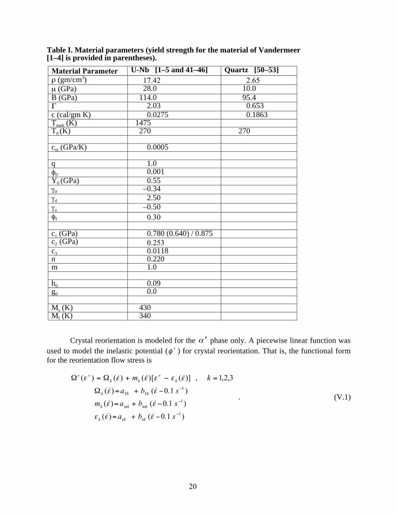
Table I. Material parameters (yield strength for the material of Vandermeer[1–4] is provided in parentheses).

Material Parameter U-Nb [1–5 and 41–46] Quartz [50–53]ρ (gm/cm3) 17.42 2.65µ (GPa) 28.0 10.0B (GPa) 114.0 95.4Γ 2.03 0.653c (cal/gm K) 0.0275 0.1863Tmelt (K) 1475T0 (K) 270 270

cm (GPa/K) 0.0005

q 1.0φ0 0.001Y0 (GPa) 0.55γ0 –0.34γd 2.50γa –0.50φf 0.30

c1 (GPa) 0.780 (0.640) / 0.875c2 (GPa) 0.253c3 0.0118n 0.220m 1.0

h0 0.09g0 0.0

Ms (K) 430Mf (K) 340

Crystal reorientation is modeled for the α ′′ phase only. A piecewise linear function wasused to model the inelastic potential ( rφ ) for crystal reorientation. That is, the functional formfor the reorientation flow stress is

)1.0()(

)1.0()(

)1.0()(

3,2,1,)]([)()()(

1

1

1

−

−

−

−+=

−+=

−+=Ω

=−+Ω=Ω

sba

sbam

sba

km

kkk

mkmkk

YkYkk

kr

kkrr

εεε

εε

εε

εεεεεε

εε &&

&&

&&

&&&

. (V.1)

21

Values for the parameters ( a b a b aYk Yk mk mk k, , , , ,ε and kbε ) in Eq. V.1 are provided in Table II for

both the materials of Cady and Vandermeer (in parentheses). Only quasi-static experiments wereavailable for the Vandermeer material. Consequently, the strain-rate effect was not modeled forthis material ( b b bYk mk k= = =ε 0). These parameters were chosen to provide a good comparison tothe uniaxial stress experiments.

Table II. Material parameters for crystal reorientation (properties for the material ofVandermeer [1–4] are provided in parentheses).

k = 1 2 3aYk (GPa) 0.04453 (0.04200) 0.23004 (0.15800) 0.40451 (0.25200)

bYk (GPa s) 1.170 × 10–4 (0.0) 0.827 × 10–4 (0.0) 0.354 × 10–4 (0.0)

amk (GPa) 35.47 (26.40) 6.61 (5.60) 16.29 (0.0)

bmk (GPa s) –6.59 × 10–3 (0.0) –7.83 × 10–4 (0.0) 1.10 × 10-5 (0.0)

a kε0.00033 (0.00030) 0.0056 (0.0047) 0.0319 (0.0214)

b kε (s) 3.85 × 10-7 (0.0) 3.95 × 10-7 (0.0) –4.90 × 10-6 (0.0)

Void nucleation has not been modeled in the existing theory. Void nucleation may beincluded by the addition of a term ( nφ& ) to Eq. III.27 [27]. Void coalescence may be included by

accelerating the rate of production of porosity after a critical value ( fφ ) is achieved [27]. In theexisting approach, however, the stiffness of a computational cell is set to zero when the stressstate reaches a surface defined in stress-triaxiality ( τ/P ), plastic strain ( pe ), and porosity (φ )space [29,38]

( )τγγγ

φφ

/exp

1

0

22

Pe

e

e

adpf

pf

p

f

−+=

=

+

. (V.2)

Values for the constants in Eq. V.2 also are provided in Table I [41].

A representative stress-versus-strain path using the proposed model is provided in Fig. 5.The conditions of uniaxial stress and a constant temperature (750 K), which is higher than themartensitic start temperature (Ms = 430 K), are imposed for this simulation. The material initiallyis in the austenitic ( 0γ ) phase. An elastic response (εe) is followed up to a stress ofapproximately 0.16 GPa. Between approximately 0.16 GPa and 0.20 GPa the deformation path iswithin the phase transformation regime (εt), where the material is converted from austenite ( 0γ )to martensite (α ′′ ). Crystal reorientation (εr) follows between 0.20 GPa and approximately 0.57GPa. The remaining part of the loading path is within the plastic regime (εp) up to a strain of0.20. The unloading path initially follows a linear elastic path (εe) followed by the transformationfrom martensite to austenite (εt) and finally, linear elastic unloading to a state of zero stress. Aresidual strain of approximately 0.125 is realized for this representative deformation.

22

0

0.1

0.2

0.3

0.4

0.5

0.6

0.7

0 0.04 0.08 0.12 0.16 0.2

Strain

ε t

εr

εe

εp

εe

εt

εe(γ0)

(α")

Figure 5. Representative mechanical response using the material model.

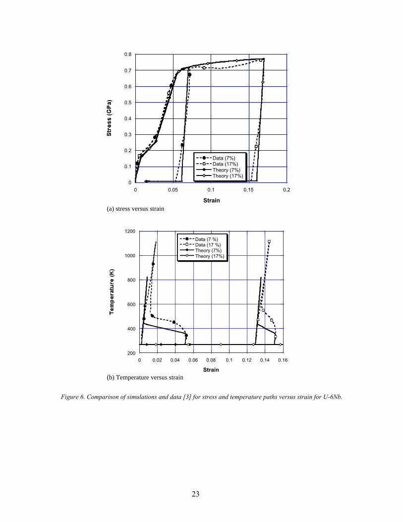
Consider the experimentally observed thermomechanical cycles [3] shown in Fig. 6. Theself-accommodated (multiple variant or twinned) α ′′ phase is loaded in tension at roomtemperature (Fig. 6a). The elastic limit is reached at a strain of approximately 0.3%, where thereorientation process is initiated. At a strain of approximately 7%, dislocation slip begins. After astrain of 7% is reached, the load is removed. A nonlinear unloading path is observed. Then thestrained specimen is heated to a temperature of 1100K (Tmax) and cooled to room temperature(Fig. 6b). The 5% strain, which remains after unloading, is recovered in two stages during thisthermal process. The initial 3% strain is recovered during the heating process, when the α ′′phase transforms back to the γ phase. Most of the heat-activated shape recovery is observed

during the heating process for the temperature range of 350 K < T < 435 K, where the α ′′ to 0γreversion occurs. Depending on the maximum amount of strain applied to the specimen, between90% to 100% of the heat-activated recovery process occurs between room temperature and 500K. This deformation and heating process is analogous to the shape memory effect. The remaining2% recovery in strain is obtained during the cooling process. Above 7% strain (Fig. 6a),irreversible deformations (dislocation slip) are observed. A loading path to 17% strain followedby unloading, heating, and cooling also is provided in Fig. 6b. The irreversible deformation maybe observed for the 17% strain experiment.

23

0

0.1

0.2

0.3

0.4

0.5

0.6

0.7

0.8

0 0.05 0.1 0.15 0.2

Data (7%)Data (17%)Theory (7%)Theory (17%)

Strain

(a) stress versus strain

200

400

600

800

1000

1200

0 0.02 0.04 0.06 0.08 0.1 0.12 0.14 0.16

Data (7 %)Data (17 %)Theory (7%)Theory (17%)

Strain(b) Temperature versus strain

Figure 6. Comparison of simulations and data [3] for stress and temperature paths versus strain for U-6Nb.

24

A comparison of the model and data [1–4] is provided in Figs. 6 a + b. A linear equation of stateis used in the simulations. The recovery strain (h0) was decreased linearly with maximum appliedstrain in the simulations. Also, h0 was degraded linearly during heating from its initial value atthe martensitic finish temperaure (Mf) to zero at the martensitic start temperature (Ms). It may beseen from Fig. 6a that the theory models the mechanical features of the experiments well. Thatis, an elastic deformation is obtained for small stress (τ < 0.042 GPa). Between 0.042 GPa and0.64 GPa, the simulated stress-versus-strain path is a result of crystal reorientation. Above 0.64GPa, the model enters the regime of slip plasticity. Unlike the experimental data, the modelpredicts a linearly elastic unloading path. Following the loading-unloading path, a heating-cooling path between room temperature and approximately 800 K was considered. Heating thestrained state between room temperature and the martensitic finish temperature results in athermal-elastic response. Between the martensitic finish (Mf = 340 K) and start (Ms = 430 K)temperatures, the transformation from α ′′ to 0γ occurs and the strain decreases with increasingtemperature. In the simulation, a thermoelastic response is obtained on further heating followedby cooling. It may be seen from Fig. 6b that the theory models the thermal responsequalitatively. The difference between the experiment and the simulation is due partly toexcluding the 0γ to γ phase transformation in the model. Also, better transformation potential

( tφ ) and kinetics (ξ& ) will improve the comparison between theory and experiment. Thethermoelastic cooling path is a result of heating above the martensitic start temperature where therecovery strain has degraded to zero.

The model was compared to data for uniaxial stress and uniaxial strain experiments forthe baseline material in Figs. 7 and 8. A comparison of model with uniaxial stress experiments isprovided in Fig. 7. A linear equation-of-state was used to generate the simulations in Fig. 7. Itmay be observed that the model compares well to both the low-strain-rate (0.1 s-1) and high-strain-rate (2000 s-1) data for U-6Nb (Fig. 7a). The elastic and reorientation (twinning) regimesare accurately modeled. The uniaxial stress simulations result in a smaller hardening response forplastic deformation, especially for the low-strain-rate simulation. This is a result of the smallerstrain and strain-rate hardening as well as larger thermal softening for the simulations. Thecomparison between the simulations and experiment in the plastic regime can be improved byreplacing the existing phenomenological flow stress ( p

sY ) model [38] with a physically based

model [47]. This will be pursued in the future. Properties for the austenitic ( 0γ ) phase were

obtained by recognizing that U-8Nb is in the 0γ phase at room temperature (Fig. 1). Setting theinitial volume fraction (ξ) to zero, the uniaxial stress simulation is compared to U-8Nb data inFig. 7b. Because room temperature was assumed for the initial state, the model predicts areorientation response to the deformation during loading. Again, a good comparison is obtainedbetween the simulation and experimental data.

25

0

0.2

0.4

0.6

0.8

1

1.2

0 0.05 0.1 0.15

Data (0.10 s-1)Data (2000 s-1)Theory (0.1 s-1)Theory (2000 s-1)

Strain

(a) U-6Nb

0

0.2

0.4

0.6

0.8

1

1.2

0 0.05 0.1 0.15

Data (1900 s-1)Theory (1900 s-1)

Strain (b) U-8Nb

Figure 7. Comparison of simulations and data for uniaxial stress experiments [5].

26

0

0.005

0.01

0.015

0.02

0.025

0 0.5 1 1.5 2 2.5 3 3.5 4

Data Theory (γ

d=2.50)

Theory (γd=1.84)

Time (µs)

(a) Impact stress of 28.4 kbar.

0

0.005

0.01

0.015

0.02

0.025

0 0.5 1 1.5 2 2.5 3 3.5 4

Data Theory (γ

d=2.50)

Time (us)

(b) Impact stress of 42.5 kbar.

0

0.005

0.01

0.015

0.02

0.025

0 0.5 1 1.5 2 2.5 3 3.5 4

DataTheory (γ

d=2.50)

Time (µs)

(c) Impact stress of 55.0 kbar.

Figure 8. Comparison of simulations and data for plate impact experiments [49].

27

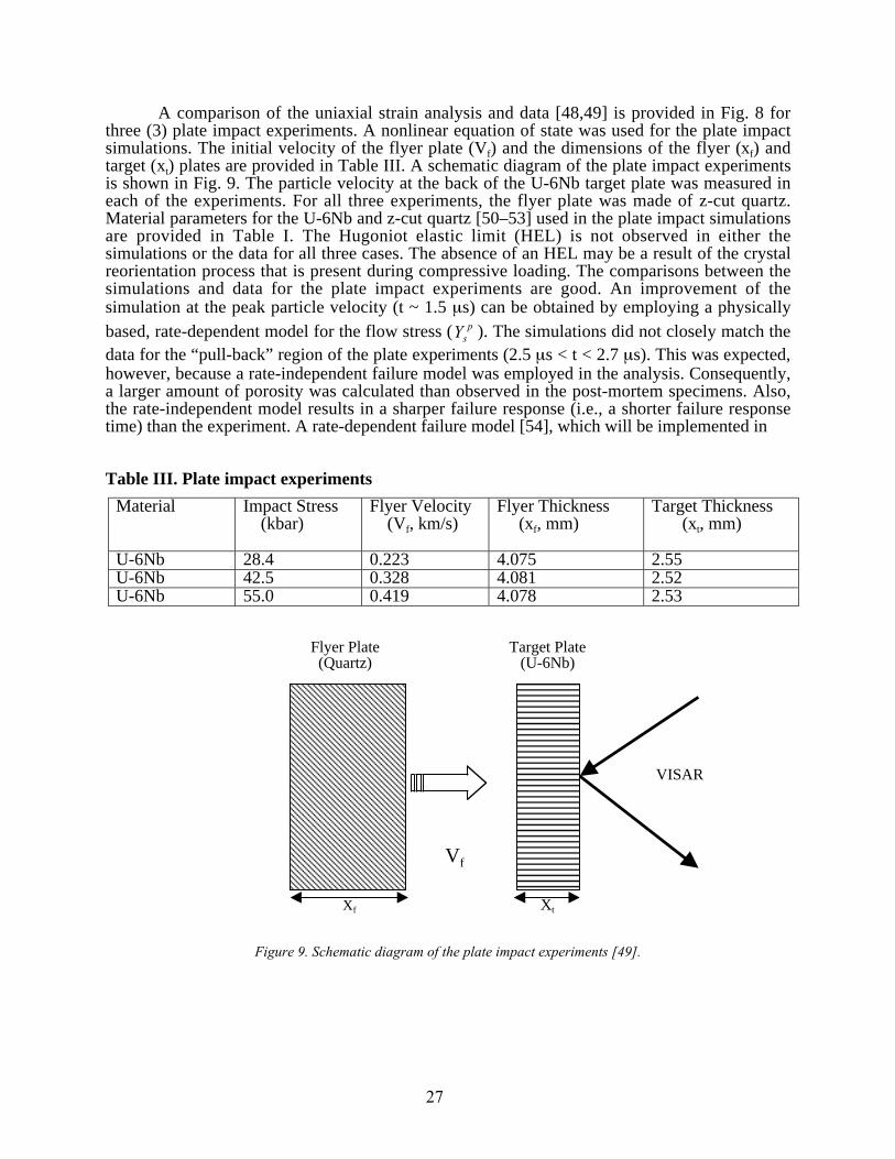
A comparison of the uniaxial strain analysis and data [48,49] is provided in Fig. 8 forthree (3) plate impact experiments. A nonlinear equation of state was used for the plate impactsimulations. The initial velocity of the flyer plate (Vf) and the dimensions of the flyer (xf) andtarget (xt) plates are provided in Table III. A schematic diagram of the plate impact experimentsis shown in Fig. 9. The particle velocity at the back of the U-6Nb target plate was measured ineach of the experiments. For all three experiments, the flyer plate was made of z-cut quartz.Material parameters for the U-6Nb and z-cut quartz [50–53] used in the plate impact simulationsare provided in Table I. The Hugoniot elastic limit (HEL) is not observed in either thesimulations or the data for all three cases. The absence of an HEL may be a result of the crystalreorientation process that is present during compressive loading. The comparisons between thesimulations and data for the plate impact experiments are good. An improvement of thesimulation at the peak particle velocity (t ~ 1.5 µs) can be obtained by employing a physicallybased, rate-dependent model for the flow stress ( p

sY ). The simulations did not closely match thedata for the “pull-back” region of the plate experiments (2.5 µs < t < 2.7 µs). This was expected,however, because a rate-independent failure model was employed in the analysis. Consequently,a larger amount of porosity was calculated than observed in the post-mortem specimens. Also,the rate-independent model results in a sharper failure response (i.e., a shorter failure responsetime) than the experiment. A rate-dependent failure model [54], which will be implemented in

Table III. Plate impact experiments

Material Impact Stress (kbar)

Flyer Velocity (Vf, km/s)

Flyer Thickness (xf, mm)

Target Thickness (xt, mm)

U-6Nb 28.4 0.223 4.075 2.55U-6Nb 42.5 0.328 4.081 2.52U-6Nb 55.0 0.419 4.078 2.53

Xf Xt

Figure 9. Schematic diagram of the plate impact experiments [49].

Vf

VISAR

Flyer Plate(Quartz)

Target Plate(U-6Nb)

28

the future, will improve the simulations in the region of material failure. Better agreementbetween theory and data also can be achieved by including a void nucleation model. In Fig. 8a,simulations for two values of the exponential coefficient ( dγ ) for the strain to failure are

provided. The larger value ( 50.2=dγ ), which was the base-line value, results in no material

failure for the simulation. The smaller value ( 84.1=dγ ) results in material failure and the

ensuing “pull-back” response of the particle velocity. The experimental data lie between thesetwo simulations. With the exception of carbides, which were crushed during the initialcompression, no damage was observed in the post-mortem specimen for the 28.4 kbarexperiment (Fig. 8a). Comparisons between the model predictions and data for the base-linevalue of 5.2=dγ are provided in Figs. 8b and 8c for impact stresses of 42.5 kbar and 55.0 kbar,

respectively.

VI. Summary

A framework for the development of a three-dimensional constitutive model that includescrystal reorientation, phase transformation, plasticity, and failure for the conditions of high strainrate has been provided. This framework was used to develop a phenomenological model that alsoincludes nonlinear elasticity (equation of state), rate-dependent plasticity, and porosity growth. Aphase diagram in stress-versus-temperature space was used to guide the solution procedure forthe material state. An implicit numerical algorithm was developed to obtain a solution to thesystem of equations for the material model. Consequently, the model imposes no additional time-step constraints on a structural analysis that utilizes the theory. The model was compared toexperimental data for uranium-niobium alloys. The numerical simulations demonstrate theability of the model to capture the effects of crystal reorientation, phase transformation, rate-dependent plasticity, and failure. Material parameters were chosen for two pedigrees of material.It was observed that loading-unloading as well as heating-cooling simulations resulted in theobserved material responses. Simulations of the model for constant temperature uniaxial stressand uniaxial strain (plate impact) experiments provided good agreement with data. Simulationswith heating and cooling experiments, however, provided only qualitative agreement. Thispoorer agreement was due, in part, to the absence of the high-temperature transformation( 0γγ − ) and the high-temperature phase (γ ). These features were omitted because of the lack ofinformation related to both the transformation and properties of the high-temperature phase ( γ ).

Better transformation potential ( tφ ) and kinetics (ξ& ) also will improve agreement betweentheory and experiments. It also was demonstrated that improved models for rate-dependentplasticity and ductile failure would result in better agreement with experimental data. Furtherimprovements to the failure model include the addition of a void-nucleation and a void-coalescence model. Improvements to the material model include a physically based, rate-dependent, flow-stress model and a rate-dependent porosity growth model. Also, improvedmodels for the degradation of the recovery strain (h0) with plastic strain and temperature will beconsidered. Future consideration will be given to kinematic hardening and the nonassociativebehavior of the inelastic strains related to crystal reorientation and phase transformation. Betterdescriptions for these inelastic strains will provide an improved material response for multipleloading and unloading deformation paths. These additions will be made as the necessary databecome available.

29

Acknowledgements

The authors are indebted to a number of individuals for providing input to this effort. E.C.Flower-Maudlin and P.J. Maudlin are acknowledged for providing programmatic support.Discussions with G.T. Gray, R.D. Field, D.J. Thoma, D. Brown, and M. Bourke related to themetallurgy of uranium-niobium alloys were invaluable. Also, the technical interactions with P.J.Maudlin, J.N. Johnson, and H.L. Schreyer are appreciated. Gratitude also is expressed toDeborah Burton, who reviewed the manuscript. This research was support by the jointDepartment of Energy (DOE) and Department of Defense (DoD) Munitions TechnologyDevelopment Program, and the DOE Accelerated Strategic Computing Initiative (ASCI).

References

1. R. A. Vandermeer, D. A. Carpenter, W. G. Northcutt, and J. C. Ogle, in Proceedings ofInternational Conference of Solid-Solid Phase Transformations, Pittsburgh, PA, 1982.

2. R. A. Vandermeer, Acta Metall. 28, 383 (1980).

3. R. A. Vandermeer, J. C. Ogle, and W. G. Northcutt, Metall. Mat. Trans. 12A, 733 (1981).

4. R. A. Vandermeer, J. C. Ogle, and W. B. Snyder, Scripta Metall. 12, 243 (1978).

5. C. M. Cady, G. T. Gray III, S. S. Hecker, D. J. Thoma, D. R. Korzekwa, R. A. Patterson, P.S. Dunn, and J. F. Bingert, in Constitutive and Damage Modeling of Inelastic Deformationand Phase Transformation, Proceedings of Plasticity, ’99, edited by A.S. Kahn (1999).

6. R. D. Field, D. J. Thoma, P. S. Dunn, D. W. Brown, C. M. Cady, Phil. Mag. A 81, 1691(2001).

7. D. W. Brown, M. A. M. Bourke, P. S. Dunn, R. D. Field, M. G. Stout, and D. J. Thoma,Metall. Mat. Trans. 32A, 2219 (2001).

8. K. Kadau, T. C. Germann, P. S. Lomdahl, and B. L. Holian, Science 296, 1681 (2002).

9. A. Saxena, T. Lookman, and A. R. Bishop, LAUR-99-0336, “Modeling of MultiscaleFunctionality in Elastic Materials,” Los Alamos National Laboratory (1999).

10. M. Huang and L. C. Brinson, J. Mech. Phys. Solids 46, 1379 (1998).

11. X. J. Gao, M. S. Huang, and L. C. Brinson, Int. J. Plast. 16, 1345 (2000).

12. M. S. Huang, X. J. Gao, and L. C. Brinson, Int. J. Plast. 16, 1371 (2000).

13. M. Paley and J. Aboudi, Mech Mater. 14, 127 (1992).

14. A. Bekker and L. C. Brinson, Mechanics of Phase Transformations and Shape MemoryAlloys, AMD-Vol. 189’ PVP-Vol. 292 (ASME, New York, 1994), p. 195.

15. L. C. Brinson, J. Intell. Mat. Systems Struct. 4, 229 (1993).

16. S. Govindjee and E. P. Kasper, Comput. Methods Appl. Mech. Eng. 171, 309 (1999).

30

17. S. Govindjee and E. P. Kasper, J. Intell. Mat. Systems Struct. 8, 815 (1997).

18. C. Liang and C. A. Rogers, J. Intell. Mater. Syst. Struct. 1, 207 (1990).

19. V. I. Levitas, Int. J. Solids Struct. 35, 889 (1998).

20. J. Lemaitre and J. L. Chaboche, Mechanics of Solid Materials (Cambridge UniversityPress, New York, 1990).

21. G. A. Maugin, The Thermomechanics of Plasticity and Fracture (Cambridge UniversityPress, New York, 1992).

22. J. Lubliner, Plasticity Theory (Macmillan Pub. Co., New York, 1990).

23. Y. C. Fung, Foundations of Solid Mechanics (Prentice-Hall Inc., Englewood Cliffs, NJ,1965).

24. M. W. Lewis and H. L. Schreyer, in High-Pressure Shock Compression of Solids II,Dynamic Fracture and Fragmentation, edited by L. Davison, D. E. Grady, and M.Shahinpoor (Springer Verlag, New York, 1996).

25. C. Liang and C. A. Rogers, J. Engr. Math. 26, 429 (1992).

26. J. G. Boyd and D. C. Lagoudas, Int. J. Plast. 12 (6), 805 (1996).

27. V. Tvergaard and A. Needleman, Int. J. Fract. 37, 197 (1988).

28. A. L. Gurson, J. Eng. Mater. Technol. 99, 2 (1977).

29. J. N. Johnson and F. L. Addessio, J. Appl. Phys. 64, 6699 (1988).

30. J. B. Leblond, G. Mottet, J. Devaux, and J. C. Devaux, Mat. Sci. Tech. 1, 815 (1985).

31. J. B. Leblond, G. Mottet, and J. C. Devaux, J. Mech. Phys. Sols. 34, 395 (1986).

32. J. B. Leblond, G. Mottet, and J. C. Devaux, J. Mech. Phys. Sols. 34, 411 (1986).

33. A. S. Oddy, J. A. Goldak, and J. M. M. McDill, Eur. J. Mech., A/Solids 9, 253 (1990).

34. Y. B. Zel’dovich and Y. P. Raizer, Physics of Shock Waves and High-TemperatureHydrodynamic Phenomena, Vol. II (Academic Press, Inc., New York, 1967).

35. L. E. Malvern, Introduction to the Mechanics of a Continuous Medium (Prentice-Hall, Inc.,Englewood Cliffs, NJ, 1969).

36. A. C. Eringen, Nonlinear Theory of Continuous Media (McGraw-Hill Book Company, Inc.,New York, 1962).

37. D. P. Flanagan and L. M. Taylor, Comp. Methods. Appl. Mech. Engr. 62, 305 (1987).

38. G. R. Johnson and W. H. Cook, Eng. Fract. Mech. 21, 31 (1985).

39. J. C. Simo and T. J. R. Hughes, Computational Inelasticity (Springer, New York, 1997).

40. N. Aravas, Int. J. Num. Methods Engr. 24, 1395 (1987).

31

41. G. R. Johnson and T. J. Holmquist, LA-11463-MS, “Test Data and ComputationalStrength and Fracture Model Constants for 23 Materials Subjected to Large Strains, HighStrain Rates, and High Temperatures,” Los Alamos National Laboratory, 1989.

42. R. L. Jackson, Rept. No. RFP-1613, The Dow Chemical Company Rocky Flats Division,Golden, CO, 1971.

43. K. H. Ecklemeyer, A. D. Romig, and L. J. Weirick, Metall. Trans. 15A, 1319 (1984).

44. R. J. Jackson and D. V. Miley, Trans. of ASME 61, 336 (1968).

45. D. R. Lowry, A. Wolfenden, and G. M. Ludtka, J. Appl. Mech. 57, 292 (1990).

46. R. J. Jackson, in The Physical Metallurgy of Uranium Alloys, edited by J. J. Burke(Brookhill, Chestnut Hill, MA, 1976), p. 611.

47. P. S. Follansbee and U. F. Kocks, Acta Metall. 30, 81 (1988).

48. D. L. Tonks, J. E.Vorthman, R. S. Hixson, A. Kelly, and A. K. Zurek, in ShockCompression of Condensed Matter-1999, edited by M. D. Furnish, L. C. Chhabildas, andR. S. Hixson (AIP, New York, 1999).

49. R. S. Hixson, J. E. Vorthman, A. K. Zurek, W. W. Anderson, and D. L. Tonks, in ShockCompression of Condensed Matter-1999, edited by M. D. Furnish, L. C. Chhabildas, andR. S. Hixson (AIP, New York, 1999).

50. J. Wackerle, J. Appl. Phys. 33, 922 (1962).

51. G. Simmons and H. Wang, Single Crystal Elastic Constants and Calculated AggregateProperties: A Handbook (The MIT Press, Cambridge, MA, 1971).

52. S. C. Jones and Y. M. Gupta, J. Appl. Phys. 88, 5671 (2000).

53. W. M. Rohsenow and J. P. Hartnett, Handbook of Heat Transfer (McGraw-Hill, NewYork, 1973).

54. F. L. Addessio and J. N. Johnson, J. Appl. Phys. 73, 1640 (1993).

This report has been reproduced directly from thebest available copy. It is available electronicallyon the Web (http://www.doe.gov/bridge).

Copies are available for sale to U.S. Departmentof Energy employees and contractors from:

Office of Scientific and Technical InformationP.O. Box 62Oak Ridge, TN 37831(865) 576-8401

Copies are available for sale to the public from:National Technical Information ServiceU.S. Department of Commerce5285 Port Royal RoadSpringfield, VA 22616(800) 553-6847