UNIVERSITY OF TARTU

Faculty of Science and Technology

Institute of Chemistry

Sinai Mwagomba

A method for thermal ambient tests of space technology equipment in a

thermal chamber - development and validation

Master’s Thesis

Supervisors

Ph.D. Riho Vendt

(Research Associate, Tartu Observatory)

Professor Ivo Leito

(Institute of Chemistry, University of Tartu)

Tartu 2014

2

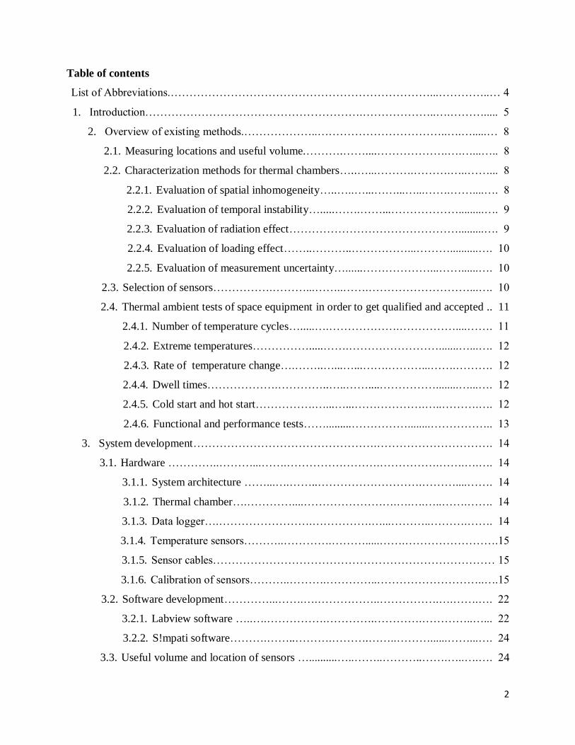
Table of contents

List of Abbreviations.……………………………………………………………...…………..… 4

1. Introduction………………………………………………….………………..….………..... 5

2. Overview of existing methods.………………..……………………………..….….....… 8

2.1. Measuring locations and useful volume.……….……....……………….….…...….. 8

2.2. Characterization methods for thermal chambers…..…...……….……….…..……... 8

2.2.1. Evaluation of spatial inhomogeneity…..…..…...……...…...…….……....…. 8

2.2.2. Evaluation of temporal instability….....…….……...……………….........…. 9

2.2.3. Evaluation of radiation effect……………………………………….........…. 9

2.2.4. Evaluation of loading effect……..………..……………...………..........…. 10

2.2.5. Evaluation of measurement uncertainty…......………………...……......…. 10

2.3. Selection of sensors…………….………...……..…….………………………...…. 10

2.4. Thermal ambient tests of space equipment in order to get qualified and accepted .. 11

2.4.1. Number of temperature cycles….....….……………….……………....……. 11

2.4.2. Extreme temperatures…………….....…….…………………….......…...…. 12

2.4.3. Rate of temperature change….……..…...…...…….………...…….………. 12

2.4.4. Dwell times……………….…………..…..……....……………........…...…. 12

2.4.5. Cold start and hot start…………….…...…...……………….…..……….…. 12

2.4.6. Functional and performance tests…….........……………........…………….. 13

3. System development………………………………………….…………………………. 14

3.1. Hardware …………..………...…….…………………….…………….…….….…. 14

3.1.1. System architecture ……...….……..……………………….………....……. 14

3.1.2. Thermal chamber….…………....…………………….….….…..…….……. 14

3.1.3. Data logger….…………………….…………….…...………..……….……. 14

3.1.4. Temperature sensors………..………….……….....…….…………………….15

3.1.5. Sensor cables………………………………………………………………… 15

3.1.6. Calibration of sensors………..……….…………..………………………..….15

3.2. Software development…………...…….….……………..…………….….…….…. 22

3.2.1. Labview software …..….…………….………….………….…………..…... 22

3.2.2. S!mpati software……….……..……….……….……..………......……...…. 24

3.3. Useful volume and location of sensors …..........…..……..………..…….…..….…. 24

3

4. Characterization of the thermal chamber ………………..……..……..……….…………. 26

4.1. Evaluation of spatial inhomogeneity ………………….…….…….……….….….…. 26

4.2. Evaluation of temporal instability ……………………...…….……..……….…...…. 28

4.2.1. Evaluation of temporal instability for the whole useful volume……….......…. 28

4.2.2. Evaluation of temporal instability at individual measuring locations………... 29

4.3. Evaluation of radiation effect ….……………………...…………….……..…….….. 30

4.4. Evaluation of loading effect ………………….…………….................................….. 31

4.5. Estimation of measurement uncertainty for temperature of the chamber………...…. 33

4.5.1. Model equation.……..…………………..................................................……. 33

4.5.2. Standard uncertainty of contributing components………….....….…….…...... 33

4.5.3. Combined standard uncertainty………………………….…..…...………….…34

4.6. Evaluation of temperature reference point on test objects..………...…………………35

4.7. Evaluation of temperature rate of change in the thermal chamber .....…...……....…. 37

5. Thermal ambient tests of sample space equipment……...……...…..……….………....…. 39

5.1. Test specimen….…….....……………………….……..…….………………..…….... 39

5.2. Summary of the thermal ambient test……………….……….…………………..…… 39

5.3. Initial functional tests…………..………….…………….…….……………………... 40

5.4. Thermal cycling………..……….…………….……….……….……………….…….. 40

5.5. Functional tests during and at the end of thermal cycling....................…..……..……. 40

6. Conclusion……….…….…..….……………...……………………………….………..….. 42

7. Summary…………….….….…………………..……….………………………………….. 43

8. List of references………….….…………………....………………………………. ……… 44

9. Kokkuvõte...............……......….….….…………...…..…………………………………..…47

10. Acknowledgements…….…........…………………...…..………….………………………. 48

11. List of appendices…………....….…………………...….……….………………………… 49

4

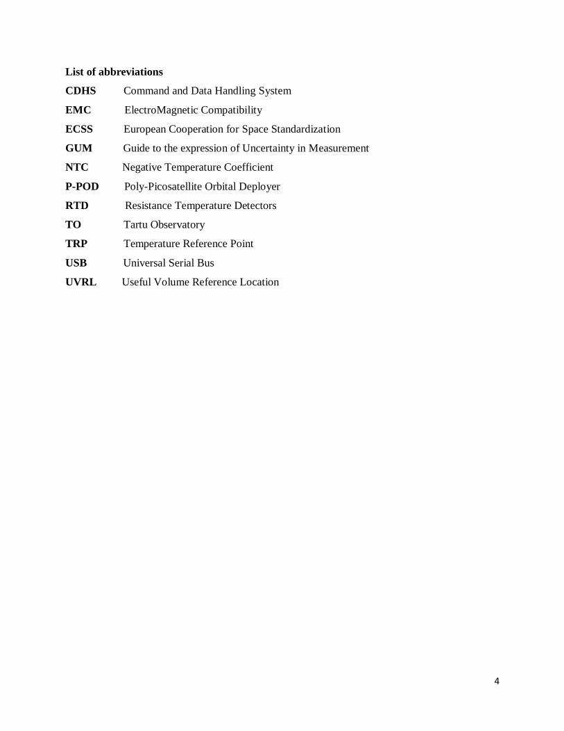
List of abbreviations

CDHS Command and Data Handling System

EMC ElectroMagnetic Compatibility

ECSS European Cooperation for Space Standardization

GUM Guide to the expression of Uncertainty in Measurement

NTC Negative Temperature Coefficient

P-POD Poly-Picosatellite Orbital Deployer

RTD Resistance Temperature Detectors

TO Tartu Observatory

TRP Temperature Reference Point

USB Universal Serial Bus

UVRL Useful Volume Reference Location

5

1. Introduction

Different pieces of equipment in life are used in various environments where other factors like

temperature, vibration, humidity, air pressure and others affect the parts that form the equipment

in distinct ways. In space, satellites make one orbit around the Earth in about 90 minutes in sun-

synchronous low earth orbit [1] which extends up to 2,000 km altitude above sea level [2]. In low

earth orbit, when the satellite faces the sun, the solar cells temperature on the external surface of

the satellite rises up to +100 °C. But when the satellite passes from the sunny side of the Earth to

the dark side, the temperature plummets to about -100 °C [3]. In short, there is a swing of about

200 °C between cold and heat in the low earth orbit in space that satellites experience in every 90

minutes. Nowadays, temperature inside the satellite is controlled in the range of (-40 … +85) °C

and nanosatellites parts and components are designed to operate in this temperature range. The

satellite sub-assemblies are therefore required to stand this temperature range [3-5]. As one goes

into the higher orbits, satellites experience even higher extreme temperatures in every rotation

when they face the sun and lower extreme temperatures when they are in the eclipse since the

satellite faces the sun as an extremely hot source of thermal radiation (about 5776 K) and also the

deep space as a very low temperature heat sink (about 3 K) [3, 6, 7]. A satellite orbiting the Earth

also has the Earth as a large source of infrared radiation [7]. Also during launching of satellites,

high temperatures are experienced by the satellites in the launching space vehicle. With such

temperature variations of very wide ranges, the parts used to build up the equipment to be used in

space must be tested to check if they will stand the effects of temperature in their lifetime in

space. If the pieces of equipment are not tested and will not stand the effects of temperature, they

will fail (get cracked and damaged) and a large amount of money, time and effort will be wasted.

In order to test the space equipment, there is a need for a controlled environment where the

parameters that affect the pieces of equipment are controlled to simulate similar values as in the

environments where the objects will be used. The environment where testing of the specimen is

to be done has to be controlled so that the samples will be tested at various specific parameters. A

climatic chamber is one of the facilities that allows selectively specified temperature and/or

relative humidity values to be realized in a closed volume in a working range. It is used for

testing different equipment under various thermal and/or relative humidity conditions. However,

one of the important problems of today’s temperature-controlled environments to users is to

6

establish with accuracy the metrological characteristics of those temperature-controlled

environments [8]. There are however a lot of factors that affect the temperature in the chamber

that lead to uncertainty of measurement results. The chamber therefore has to be characterized in

order to precisely validate the performance and the influence of all factors that affect the

temperature in the chamber and to know its working conditions. It is also difficult to characterize

climatic chambers using a manual way as it requires many temperature sensors from which

temperature values have to be taken simultaneously and at short intervals for example, a

minimum of nine sensors for climatic chambers of volume of less than 2000 liters [9].

To date, standard guidelines have been established by European Cooperation for Space

Standardization (ECSS) in Space Engineering Testing standard [4] giving requirements to be met

for space equipment testing. The required temperature margins for thermal ambient testing of

space equipment are specified. For equipment to be used in space, thermal ambient tests are

required to be carried out to meet the temperature margin of ±5 °C in the measurement range

[10]. These margins have to be accurately met if space missions are to be successful. However,

the standard does not describe how the requirements can be achieved through testing. For the

purpose of thermal ambient testing of space equipment at Tartu Observatory (TO), a commercial

thermal chamber was procured. This device has to be investigated in order to compile uncertainty

budget as is usually the case with most commercial equipment. The characteristics that contribute

to temperature measurement uncertainty need to be validated. The chamber cannot be used as it

is, without being checked, for such a purpose of space equipment testing which require to meet

the specified requirements before satellites can be accepted for launching. All required

parameters that affect operation of satellites in space [10], including temperature, need to be

tested before launching. Once a satellite is launched, there is no way to modify its hardware. It is

of paramount importance that equipment to be used for testing be characterized with specific

loads as will be analyzed by the user, preferably in the environment where application will

actually be done.

The main objective of this thesis is to develop a method for thermal ambient testing of space

equipment that meets the requirements of the above mentioned standard [10]. The goal includes:

7

i. selecting and installing suitable temperature sensors in the climatic chamber, and

connecting them to computer via data logger,

ii. developing a software for data acquisition,

iii. characterizing the climatic chamber to be used for thermal ambient testing of

space equipment,

iv. evaluating temperature measurement uncertainty budget for specific loads that

will be tested at TO,

v. testing a sample space equipment using the developed method and its estimated

uncertainty.

The climatic chamber to be characterized enables creating environment with controlled

parameters, such as temperature and relative humidity. The scope of this study is only the

temperature characterization of the chamber and the relative humidity characterization of the

chamber is not carried out. The chamber is hence herein referred to as a thermal chamber. During

testing of sample space technology equipment, there is need to conduct functional tests of the

sample space equipment under test to check its functionality during testing. The functional tests

depend on the particular equipment that is being tested and are out of the scope of this study.

This thesis has five chapters. Chapter 2 gives the literature review of the subject. Chapter 3

discusses the system development for this method. The characterization procedure for the thermal

chamber and its results are given in Chapter 4. Chapter 5 discusses the thermal ambient testing of

sample space technology equipment using the method. Chapter 6 gives the conclusions and

recommendations for improvement. Drawings and schemes are given in the appendices.

8

2. Overview of existing methods

2.1 Measuring locations and useful volume

As a rule, calibrations are carried out through measurements in several locations in the useful

volume [9]. The useful volume of a thermal chamber is the partial volume of the thermal chamber

spanned by the measuring locations of the sensors used for calibration. According to the

arrangement of the measuring locations, the useful volume can considerably differ from the total

volume of the chamber. The calibration of the chamber is valid only for this useful volume [9].

Spatial interpolation of the determined values is permissible only for the workspace. The

extrapolation of the measurement results outside the workspace is not allowed [8]. A measuring

location is the spatial position in which a temperature sensor is arranged in the useful volume for

calibration. A measuring location thus is a small volume which is defined by the dimensions of

the sensor elements [9]. For greater useful volumes, the measuring locations are to be arranged in

the useful volume in the form of a cubic lattice with a maximum lattice constant of 1 m [9].

2.2. Characterization methods for thermal chambers

There are three main ways how thermal chambers can be characterized: 1) unloaded, 2) loaded,

and 3) characterization in individual sensor locations in the thermal chamber [9]. The process of

characterization of unloaded chamber relates to the empty useful volume spanned by the

measuring locations in the thermal chamber and to the useful volume with a test object in the

loaded thermal chamber characterization method. Characterization in individual sensor locations

relates to each location idependently without covering the whole useful volume. All these

methods cover the evaluation of:

i. spatial inhomogeneity,

ii. temperature instability,

iii. radiation effect,

iv. loading effect.

2.2.1 Evaluation of spatial inhomogeneity

Spatial inhomogeneity is expressed as the maximum deviation of the temperature of a corner or

wall measuring location from the reference location of the useful volume i.e. the center of the

working space [9].

9

2.2.2 Evaluation of temporal instability

Temporal instability for air temperature is evaluated from the registration of the temporal

variation of temperature over a period of time of at least 30 minutes after steady-state conditions

have been reached. Steady-state conditions are considered to be reached when systematic

variations of temperature are no longer observed [9]. For the measurement of the temporal

instability, at least 30 measurement values are to be recorded in 30 minutes at more or less

constant time intervals. The measurement needs to be performed at least for the center of the

useful volume or for the reference measuring location and for each calibration temperature [9].

2.2.3 Evaluation of radiation effect

At air temperatures in the thermal chamber differing from ambient temperature, the inner wall of

the chamber always has a temperature which deviates from the air temperature [9]. The

temperature sensors and indeed the test objects in the thermal chamber therefore have a slightly

different temperature from the air temperature due to radiation effect. The difference between

these two temperatures depends on the surface emissivity, size and position of the sensor in the

chamber. It also depends on speed of air at the sensor and the difference between air temperature

and thermal chamber wall temperature [9]. There are three ways how the radiation effect on

temperature in thermal chambers can be evaluated:

i. using two calibrated sensors, one with high emissivity and another with low emissivity in

the reference location of the useful volume. The temperature read by a sensor with low

emissivity represents chamber air temperature without radiation effect and the sensor with

high emissivity slightly indicates the temperature with radiation effect.

ii. using two similar calibrated sensors, one with a radiation shield applied and another

without a shield in the reference location of the working space. The sensor without a

radiation shield measures the temperature with radiation effect and the sensor with a

radiation shield reads the temperature which is not affected by radiation.

iii. recording the wall temperature and there after an approximate air temperature with a

sensor with low emissivity or with radiation shield.

In this task, the radiation effect was evaluated by method ii. because it does not require the exact

emissivity of the sensors to be known and no special sensors are needed for the purpose as is

10

required in method i. The last method can easily introduce errors as it is not easy to differentiate

wall temperature with air temperature with exactness as they affect each other all the time.

2.2.4 Evaluation of loading effect

The loading effect is defined as the maximum average value when the differences between the

average maximum temperatures achieved between the empty chamber and the loaded chamber

from each measurement location are calculated and when the difference between minimum

temperatures achieved between the empty chamber and the loaded chamber from each

measurement location are calculated [8]. A calibration is carried out at least for the reference

measuring location with and without load, and the maximum difference is taken as the half-width

of a rectangularly distributed uncertainty contribution [9]. Thermal chambers are normally

calibrated and characterized in the empty state [9]. The investigation of the loading effect can be

performed with a customer-specific load or using a test load, the volume of the latter amounting

at least to 40 % of the useful volume [8].

2.2.5 Evaluation of measurement uncertainty

The combined uncertainty to be evaluated is composed of the uncertainty of the measurement of

temperature using the reference measuring sensors, the contributions of the temperature

instability, radiation effect, influence of ambient conditions, temperature inhomogeneity, as well

as the loading effect [8, 9, 11].

2.3. Selection of sensors

There are many different types of sensors available for measuring temperature. The three most

common types are 1) resistance temperature detectors (RTDs), 2) thermocouples (TCs), and 3)

thermistors. Each of them have specific operating parameters that may make it a better choice for

some applications than others. There are several considerations when selecting a temperature

sensor [12]. Some of the factors are:

i. Type of application,

ii. Cost budget per sensor,

iii. Distance from sensor to the display,

11

iv. Measurement range. A sensor must be able to withstand the temperature without

getting damaged by heat. Different sensors are sheathed with different materials to

suit the temperature range they are measuring. Also sensors perform well in their

measuring range.

v. Size of sensors. Sensors come in different sizes and shapes and the one that fits the

specific purpose is chosen.

vi. Data acquisition methods

2.4. Thermal ambient tests of space equipment in order to get qualified and accepted

For space equipment to qualify and get accepted for launching, it has to pass a series of

pre-launch tests in qualification and acceptance tests stages [10]. Thermal ambient test is one of

the environmental tests done in both the qualification and acceptance stages. An environmental

test is a test conducted on flight or flight configured hardware to assure that the flight hardware

will perform satisfactorily in one or more of its flight environments. Examples are acoustic,

thermal vacuum and electromagnetic compatibility (EMC) tests. Environmental testing is

normally combined with functional testing to a degree which depends on the objectives of the test

[13].

Thermal ambient test is carried out to ensure that the specimen design withstands the

environment it will encounter during launching and during its lifetime in space without

degradation of its performance [10]. It determines the ability of components, equipment or other

articles to withstand rapid changes of ambient temperature and also its ability to withstand the

maximum and minimum temperatures it experiences during its operation [10, 13]. Thermal

ambient testing consists of thermal cycling the entire experiment assembly in an operating mode.

This test is performed to detect problems early in the hardware development. It checks the

functional capability of the electronic components in a simulated on-orbit temperature

environment [14].

2.4.1 Number of temperature cycles

Temperature cycles refer to the transition from an initial temperature to the same temperature,

with excursion within a specified range [10]. The number of thermal cycles to be carried out

12

depends on whether the test is qualification test or acceptance test. For equipment to be launched

in space, it is required that the specimen shall be subjected to 8 temperature cycles in one

qualification test and 4 cycles in one acceptance test according to ECSS space engineering testing

standard [10].

2.4.2. Extreme temperatures

Extreme operating conditions refer to conditions that a measuring instrument or measuring

system is required to withstand without damage, and without degradation of specified

metrological properties, when it is subsequently operated under its rated operating conditions

[15]. For equipment to be launched in space, the temperature cycles are required to span from

extreme temperatures of -40 °C as lowest extreme temperature and +85 °C as highest extreme

temperature [3-5].

2.4.3. Rate of temperature change

The rate of temperature change refers to the speed at which the temperature in the thermal

chamber increases or decreases while thermal cycling the specimen under test. For equipment to

be launched in orbit the rate of temperature change is required to be less than 20 K/min [5].

2.4.4. Dwell times

Dwell times refer to the duration necessary to ensure that internal parts or subassembly of a space

segment equipment have achieved thermal equilibrium, from the start of temperature stabilization

phase, i.e. when the temperature reaches the targeted test temperature plus or minus the test

tolerance [10]. For equipment to be launched in space, the specimen is required to be exposed to

dwell times of at least 2 hours at each extreme temperature in thermal ambient tests [10].

2.4.5. Cold start and hot start

Cold start refers to switching on the specimen into operational mode at the minimum extreme

temperature. Hot start refers to switching on the specimen into operational mode at the

maximum extreme temperature. The specimen shall be tested for cold start at the minimum

extreme temperature to check for cold start capability and also for hot start at maximum extreme

13

temperature to check for hot start capability of the specimen. Both cold and hot starts shall be

performed at the end of dwell times. The test starts with the specimen off. [14]

2.4.6. Functional and performance tests

Functional testing is a series of electrical or mechanical tests conducted on flight or flight

configured hardware at conditions equal or less than design specifications. Its purpose is to

establish that the hardware performs satisfactorily in accordance with the design specifications

[16]. Depending on the situation, and the type of equipment under test, there are various

functional tests of various complications and depth [16]. Functional and performance tests shall

be performed before the start and after the thermal ambient test. They shall also be performed as

a minimum at hot and cold operating temperatures and during the whole duration of respective

number of cycles at the end of each dwell time. Functional and performance tests for space

equipment to be launched in low earth orbit shall only start after a dwell time greater or equal to 2

hours at the maximum and minimum extreme temperatures [9, 16]. The specimen shall be

visually examined and electrically and mechanically checked as required by the relevant

specification [17].

14

3. System development

3.1. Hardware

3.1.1. System architecture

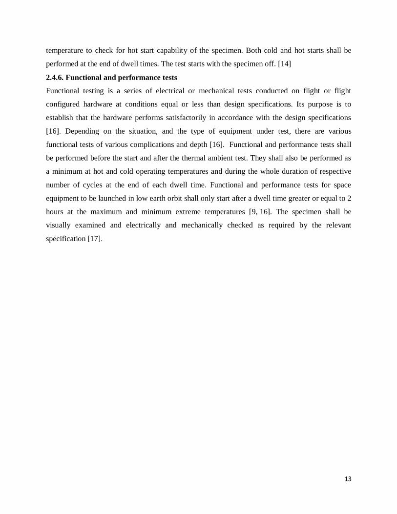
The system setup of the method for thermal ambient tests in the thermal chamber is presented in

the system architecture in Figure 1.

Figure 1. System architecture.

Temperature data from the thermal chamber is logged into a computer file using the Labview

software program via a data logger. The thermal chamber is controlled and the desired parameters

are set using the S!mpati software [18].

3.1.2. Thermal chamber

A Weisstechnik WKL 64 thermal chamber at Tartu Observatory was automated and its useful

volume was characterized using the unloaded chamber characterization method with the loading

effect evaluated. It has operational temperature range of -40 °C to +180 °C. The chamber has

internal dimensions of height 400 mm, width of 470 mm and depth of 345 mm [19].

3.1.3 Data logger

A commercial Measurement Computing USB Temp data logger is used in this task. It supports

data acquisition from thermocouples, RTDs and thermistors. The logger has the capability to read

two samples per second. It supports Visual Studio, Java, Labview and DASYLab programming

environments. It can acquire temperature and voltage data from the sensors [20].

15

3.1.4. Temperature sensors

In this topic, the sensors used had to meet the following requirements:

i. Very small size sensors. Small size sensors enable fast time response. Small sensors

can also be installed even in very small areas.

ii. Sensors that work in temperature range of -40 °C to +85 °C.

iii. Accuracy ±1%.

iv. Resolution 0.01 °C.

v. Long term stability < 0.1 °C / year.

vi. Fast time response.

Different types of thermocouples, RTDs and thermistors were analyzed and the best choice of the

sensors for the purpose were miniature thermistors. An NTC EPCOS B57861S302F40 miniature

thermistor was chosen for this task. It has working range of -55 °C to +155 °C and diameter of

2.4 mm and meets the specified technical requirements given above [21].

3.1.5. Sensor cables

In order to conduct this study there was a need for cables that could stand the maximum and

minimum extreme temperatures (from -40 °C to +85 °C) without getting damaged and that would

have the size that would suit the miniature sensors chosen. Miniature Nexans - 157284 coaxial

cable was chosen for the purpose. The cable has copper conductor plated with silver with

Fluorinated Ethylene Propylene jacket material and has operating temperature range from -90 °C

to +200 °C. The outside diameter of the cable is 1.17 mm [22]. The cables were soldered to the

sensors and the connection pins were soldered at the other end of the cables for connecting the

sensors to data logger. Thermo shrink was used to cover the joints.

3.1.6. Calibration of sensors

Thermistors work on the principle that a change in temperature causes a change in the resistance

of the sensors. However the relationship between temperature and resistance is not linear. There

was a need to calibrate the sensors. The temperature‐resistance curve of thermistors can be

described by different equations. The most commonly used equation is the Steinhart-

Hart Equation shown below [23].

16

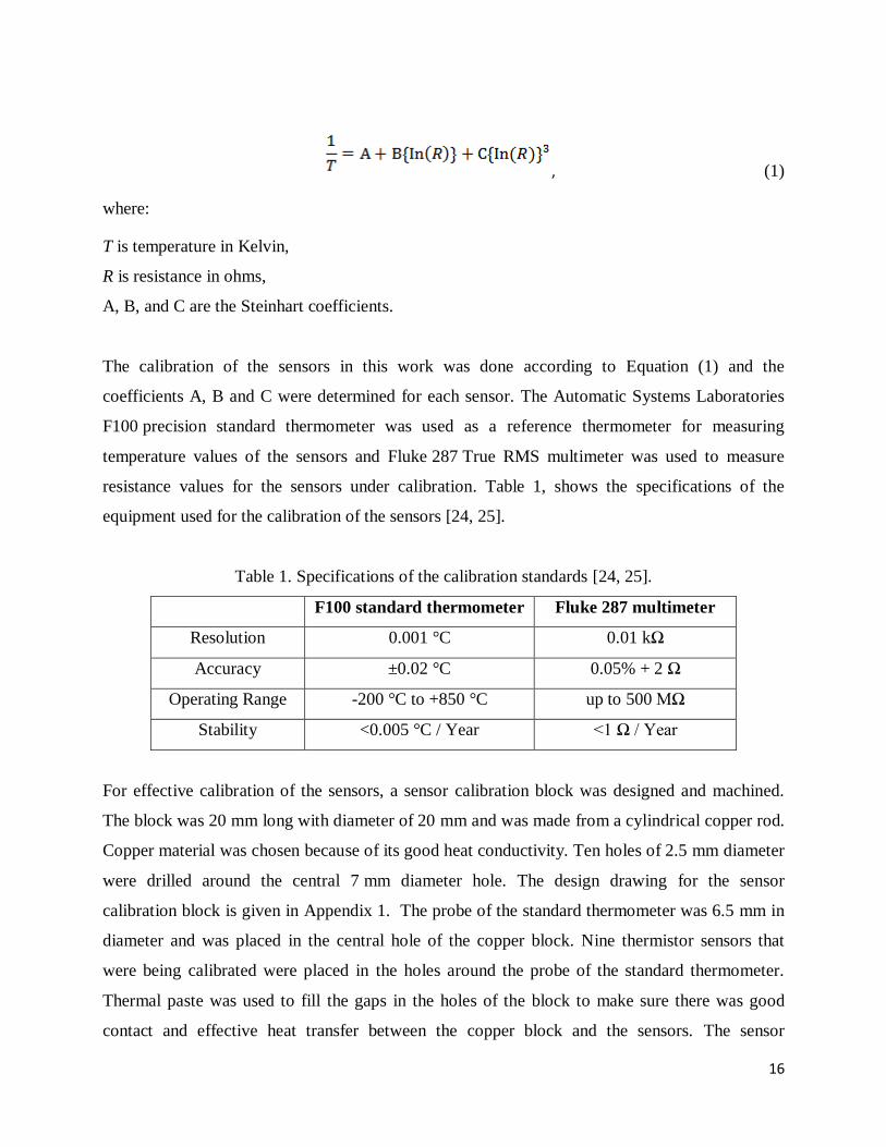
, (1)

where:

T is temperature in Kelvin,

R is resistance in ohms,

A, B, and C are the Steinhart coefficients.

The calibration of the sensors in this work was done according to Equation (1) and the

coefficients A, B and C were determined for each sensor. The Automatic Systems Laboratories

F100 precision standard thermometer was used as a reference thermometer for measuring

temperature values of the sensors and Fluke 287 True RMS multimeter was used to measure

resistance values for the sensors under calibration. Table 1, shows the specifications of the

equipment used for the calibration of the sensors [24, 25].

Table 1. Specifications of the calibration standards [24, 25].

F100 standard thermometer Fluke 287 multimeter

Resolution 0.001 °C 0.01 kΩ

Accuracy ±0.02 °C 0.05% + 2 Ω

Operating Range -200 °C to +850 °C up to 500 MΩ

Stability <0.005 °C / Year <1 Ω / Year

For effective calibration of the sensors, a sensor calibration block was designed and machined.

The block was 20 mm long with diameter of 20 mm and was made from a cylindrical copper rod.

Copper material was chosen because of its good heat conductivity. Ten holes of 2.5 mm diameter

were drilled around the central 7 mm diameter hole. The design drawing for the sensor

calibration block is given in Appendix 1. The probe of the standard thermometer was 6.5 mm in

diameter and was placed in the central hole of the copper block. Nine thermistor sensors that

were being calibrated were placed in the holes around the probe of the standard thermometer.

Thermal paste was used to fill the gaps in the holes of the block to make sure there was good

contact and effective heat transfer between the copper block and the sensors. The sensor

17

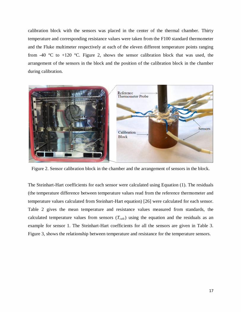
calibration block with the sensors was placed in the center of the thermal chamber. Thirty

temperature and corresponding resistance values were taken from the F100 standard thermometer

and the Fluke multimeter respectively at each of the eleven different temperature points ranging

from -40 °C to +120 °C. Figure 2, shows the sensor calibration block that was used, the

arrangement of the sensors in the block and the position of the calibration block in the chamber

during calibration.

Figure 2. Sensor calibration block in the chamber and the arrangement of sensors in the block.

The Steinhart-Hart coefficients for each sensor were calculated using Equation (1). The residuals

(the temperature difference between temperature values read from the reference thermometer and

temperature values calculated from Steinhart-Hart equation) [26] were calculated for each sensor.

Table 2 gives the mean temperature and resistance values measured from standards, the

calculated temperature values from sensors (Tcalc) using the equation and the residuals as an

example for sensor 1. The Steinhart-Hart coefficients for all the sensors are given in Table 3.

Figure 3, shows the relationship between temperature and resistance for the temperature sensors.

18

Table 2. Example of the calibration data for Sensor 1.

T / °C R / Ω T / K 1/T mK-1

InR / Ω In(R)3 / Ω

3 Tcalc / °C Res / °C

-40.896 112480.000 231.895 4.312 11.631 1573.253 -40.883 0.013

-31.479 59500.000 241.671 4.318 10.994 1328.726 -31.525 -0.046

-20.740 30720.000 252.410 3.962 10.333 1103.158 -20.693 0.047

-10.509 17190.000 262.641 3.807 9.752 927.454 -10.479 0.030

-0.414 10078.000 272.736 3.667 9.218 783.296 -0.440 -0.026

23.123 3305.300 296.064 3.378 8.103 532.087 23.039 -0.084

40.218 1581.900 313.368 3.191 7.366 399.726 40.236 0.018

60.385 735.200 333.535 2.998 6.600 287.515 60.403 0.018

84.663 303.450 359.880 2.827 5.715 186.680 84.793 0.130

100.560 200.900 373.710 2.676 5.303 149.114 100.564 0.004

120.711 115.410 393.861 2.539 4.748 107.070 120.604 -0.107

Steinhart coefficients / °C-1

C B A

8.410311×10-8

2.395800×10-4

1.392714×10-3

Table 3. Steinhart-Hart coefficients for the sensors.

Steinhart – Hart coefficients

Sensor A / °C -1

B / °C -1

C / °C -1

1 1.392714×10-3 2.395800×10

-4 8.410311×10

-8

2 1.389369×10-3 2.402207×10

-4 8.103822×10

-8

3 1.391608×10-3 2.396213×10

-4 8.384731×10

-8

4 1.391828×10-3 2.398144×10

-4 8.333081×10

-8

5 1.394587×10-3 2.393127×10

-4 8.601122×10

-8

6 1.391608×10-3 2.396213×10

-4 8.384731×10

-8

7 1.391046×10-3 2.398763×10

-4 8.340808×10

-8

8 1.391398×10-3 2.397475×10

-4 8.343215×10

-8

9 1.391446×10-3 2.397680×10

-4 8.327609×10

-8

Figure 3. Example of the temperature-resistance relationship for sensor 1.

19

The residuals for each sensor were evaluated from the mean temperature values calculated from

the Steinhart-Hart equation and the temperature valus measured by the standard themometer at

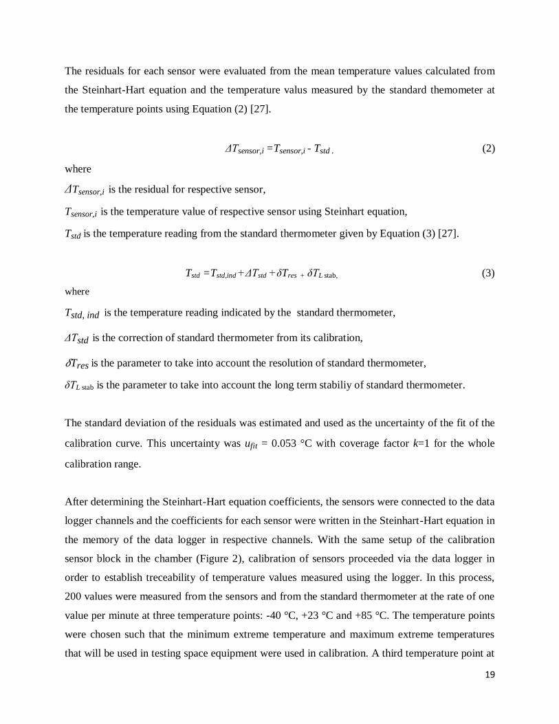
the temperature points using Equation (2) [27].

ΔTsensor,i =Tsensor,i - Tstd , (2)

where

ΔTsensor,i is the residual for respective sensor,

Tsensor,i is the temperature value of respective sensor using Steinhart equation,

Tstd is the temperature reading from the standard thermometer given by Equation (3) [27].

Tstd =Tstd,ind +ΔTstd +δTres + δTL stab, (3)

where

Tstd, ind is the temperature reading indicated by the standard thermometer,

ΔTstd is the correction of standard thermometer from its calibration,

𝛿Tres is the parameter to take into account the resolution of standard thermometer,

δTL stab is the parameter to take into account the long term stabiliy of standard thermometer.

The standard deviation of the residuals was estimated and used as the uncertainty of the fit of the

calibration curve. This uncertainty was ufit = 0.053 °C with coverage factor k=1 for the whole

calibration range.

After determining the Steinhart-Hart equation coefficients, the sensors were connected to the data

logger channels and the coefficients for each sensor were written in the Steinhart-Hart equation in

the memory of the data logger in respective channels. With the same setup of the calibration

sensor block in the chamber (Figure 2), calibration of sensors proceeded via the data logger in

order to establish treceability of temperature values measured using the logger. In this process,

200 values were measured from the sensors and from the standard thermometer at the rate of one

value per minute at three temperature points: -40 °C, +23 °C and +85 °C. The temperature points

were chosen such that the minimum extreme temperature and maximum extreme temperatures

that will be used in testing space equipment were used in calibration. A third temperature point at

20

normal room temperature (+23 °C ) was also chosen in the middle of the calibration range. The

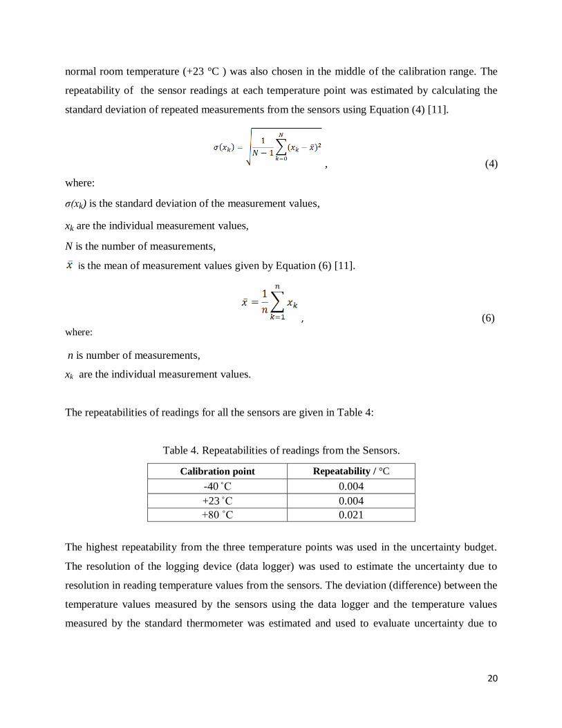
repeatability of the sensor readings at each temperature point was estimated by calculating the

standard deviation of repeated measurements from the sensors using Equation (4) [11].

, (4)

where:

σ(xk) is the standard deviation of the measurement values,

xk are the individual measurement values,

N is the number of measurements,

is the mean of measurement values given by Equation (6) [11].

, (6)

where:

n is number of measurements,

xk are the individual measurement values.

The repeatabilities of readings for all the sensors are given in Table 4:

Table 4. Repeatabilities of readings from the Sensors.

Calibration point Repeatability / °C

-40 ˚C 0.004

+23 ˚C 0.004

+80 ˚C 0.021

The highest repeatability from the three temperature points was used in the uncertainty budget.

The resolution of the logging device (data logger) was used to estimate the uncertainty due to

resolution in reading temperature values from the sensors. The deviation (difference) between the

temperature values measured by the sensors using the data logger and the temperature values

measured by the standard thermometer was estimated and used to evaluate uncertainty due to

21

temperature gradient between the standard thermometer and the sensors [26]. This uncertainty

was ugrad = 0.14 °C for the whole temperature range. The long term stability for the sensors

(L stab= 0.3 ˚C / year) was given in the sensor manufacturer´s data sheet. The standard

thermometer used had the resolution of 0.001 °C, expanded uncertainty of 0.02 °C at 95%

confidence level with coverage a factor k=2 from its calibration certificate and long term stability

of 0.005 °C /year. The combined standard uncerainty of each sensor at every calibration point

was found by combining the uncertainty due to repeatability of measurements from the sensors,

uncertainty of the fit of calibration graph, the resolution of the measurements from the sensors,

long term stability of the sensors, temperature gradient between the standard thermometer and

sensors and the contributions due to resolution, calibration uncertainty and the long term stability

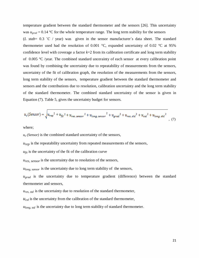
of the standard thermometer. The combined standard uncertainty of the sensor is given in

Equation (7). Table 5, gives the uncertainty budget for sensors.

, (7)

where;

uc (Sensor) is the combined standard uncertainty of the sensors,

urep is the repeatability uncertainty from repeated measurements of the sensors,

ufit is the uncertainty of the fit of the calibration curve

ures, sensor is the uncertainty due to resolution of the sensors,

ulong, sansor is the uncertainty due to long term stability of the sensors,

ugrad is the uncertainty due to temperature gradient (difference) between the standard

thermometer and sensors,

ures, std is the uncertainty due to resolution of the standard thermometer,

ucal is the uncertainty from the calibration of the standard thermometer,

ulong, std is the uncertainty due to long term stability of standard thermometer.

22

Table 5. Uncertainty budget for the sensors

Quantity

Source of uncertainty

Uncertainty

/ °C

Distribution

Sensitivity

coefficient

Standard

uncertainty

/ °C

urep sensor repeatability 0.021 normal 1 0.021

ures, sensor sensor resolution 0.00001 rectangular 1 0.000006

ufit calibration curve fit 0.053 normal 1 0.053

ulong, sensor sensor long term stability 0.3 rectangular 1 0.173

ugrad

gradient between standard

thermometer and sensors

0.14

rectangular

1

0.1

ures, std standard thermometer

resolution

0.001 rectangular 1 0.0003

ucal standard thermometer

standard uncertainty k=1

0.01 normal 1 0.01

ulong, std standard thermometer long

term stability

0.005 °C

/year

rectangular 1 0.003

The evaluated combined standard uncertainty of all the sensors is 0.2 °C for the entire

measurement range (-40 … 85) °C.

3.2. Software development

In order to characterize the thermal chamber and during thermal ambient testing of space

equipment, data must be acquired from the sensors in the thermal chamber. There is also a need

to control the thermal chamber as desired. A computer was used in data acquisition and

controlling of the chamber. Software programs were therefore developed and used for the

purpose.

3.2.1. Labview sofware

A custom made software was developed by using the tools of Labview for data acquisition using

a computer from the sensors via a data logger. The software makes it possible to acquire data

virtually simultaneously form multiple sensors via the data logger. This is useful because in order

to effectively characterize the thermal chamber, and also when testing space equipment,

temperature values from multiple sensors need to be taken at virtually same time, at the same rate

and within the same time duration. The program makes it possible to set the time interval when

data should be acquired. The trends of data acquisition can be seen graphically from the front

23

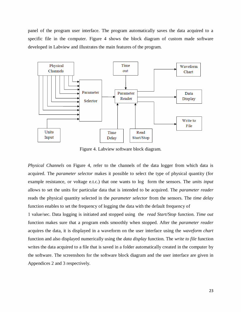
panel of the program user interface. The program automatically saves the data acquired to a

specific file in the computer. Figure 4 shows the block diagram of custom made software

developed in Labview and illustrates the main features of the program.

Figure 4. Labview software block diagram.

Physical Channels on Figure 4, refer to the channels of the data logger from which data is

acquired. The parameter selector makes it possible to select the type of physical quantity (for

example resistance, or voltage e.t.c.) that one wants to log form the sensors. The units input

allows to set the units for particular data that is intended to be acquired. The parameter reader

reads the physical quantity selected in the parameter selector from the sensors. The time delay

function enables to set the frequency of logging the data with the default frequency of

1 value/sec. Data logging is initiated and stopped using the read Start/Stop function. Time out

function makes sure that a program ends smoothly when stopped. After the parameter reader

acquires the data, it is displayed in a waveform on the user interface using the waveform chart

function and also displayed numerically using the data display function. The write to file function

writes the data acquired to a file that is saved in a folder automatically created in the computer by

the software. The screenshots for the software block diagram and the user interface are given in

Appendices 2 and 3 respectively.

24

3.2.2. S!mpati software

For setting and controlling the thermal chamber parameters, a S!mpati software version 4.06

provided by manufacturer of the thermal chamber was used [18]. Two programs for thermal

cycling were created within S!mpati software using the S!mpati Symbolic editor, one for

qualification and the other one for acceptance thermal ambient tests. The programs are used to set

maximum and minimum extreme temperatures of the tests and the dwell times at the extreme

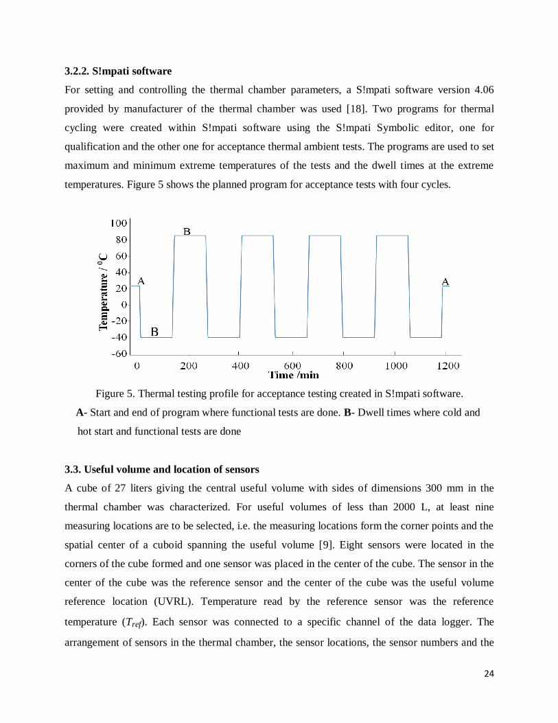
temperatures. Figure 5 shows the planned program for acceptance tests with four cycles.

Figure 5. Thermal testing profile for acceptance testing created in S!mpati software.

A- Start and end of program where functional tests are done. B- Dwell times where cold and

hot start and functional tests are done

3.3. Useful volume and location of sensors

A cube of 27 liters giving the central useful volume with sides of dimensions 300 mm in the

thermal chamber was characterized. For useful volumes of less than 2000 L, at least nine

measuring locations are to be selected, i.e. the measuring locations form the corner points and the

spatial center of a cuboid spanning the useful volume [9]. Eight sensors were located in the

corners of the cube formed and one sensor was placed in the center of the cube. The sensor in the

center of the cube was the reference sensor and the center of the cube was the useful volume

reference location (UVRL). Temperature read by the reference sensor was the reference

temperature (Tref). Each sensor was connected to a specific channel of the data logger. The

arrangement of sensors in the thermal chamber, the sensor locations, the sensor numbers and the

25

data logger channels to which the sensors were connected are given in Figure 6 where Li is the

location number, Si is the sensor number and Ci is the data logger channel number.

Figure 6. Sensor locations in the thermal chamber.

26

4. Characterization of the thermal chamber

In order to meet the specific objectives in characterizing the thermal chamber, a step by step

method of how results were obtained, results and discussions are given for each parameter. The

characterization of the thermal chamber was done in the temperature range of -40 °C to +85 °C.

The range was chosen on the basis that the minimum and maximum measuring extreme

temperatures for testing space equipment were chosen and the third one at normal room

temperature (+23 °C) was also chosen. The factors that contribute to the measurement

uncertainty of temperature measurements in the thermal chamber including temperature

inhomogeneity, temperature instability, radiation effect and loading effect were evaluated. The

temperature rate of change in the thermal chamber was also evaluated with different loading

setups typical of loads that will be tested.

4.1. Evaluation of spatial inhomogeneity

In this thesis the spatial inhomogeneity was evaluated as the maximum deviation of temperature

of each of the eight corners of the cube where the sensors are located from the central reference

sensor. Temperature values were taken from each sensor and spatial inhomogeneity was

evaluated from the mean values of each sensor and the mean values of the reference sensor where

spatial inhomogeneity is given by Equation (8) [9].

|δTinhom| ≤ Max|Tref - Ti | , (8)

where:

δTinhom is the temperature inhomogeneity,

Tref is the reference sensor mean temperature,

Ti is the mean temperature from any specific location.

The deviation of each sensor from the reference location L9 are given in Table 6. Spatial

inhomogeneity results for the three temperature locations according to Equation (8) are given in

Table 7.

27

Table 6. Temperature deviations of locations from the reference location, L9 (Figure 6).

Measurement

location Deviation from reference location / °C

-40 °C +23 °C +85 °C

L1 .0.04 -0.18 -0.83

L2 -0.63 -0.52 -0.56

L3 .0.43 .0.09 -0.87

L4 .0.50 .0.09 -0.97

L5 .0.36 .0.01 .0.19

L6 -0.44 -0.20 -0.06

L7 -0.45 -0.14 .0.01

L8 .0.16 .0.07 -0.40

Table 7. Spatial inhomogenities.

Temperature point -40 °C +23 °C +85 °C

Spatial inhomogeneity / °C 0.63 0.52 0.97

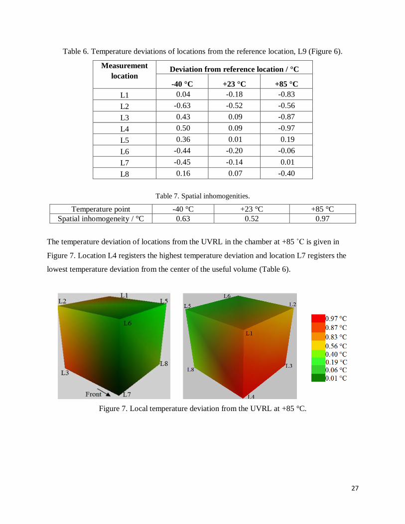
The temperature deviation of locations from the UVRL in the chamber at +85 ˚C is given in

Figure 7. Location L4 registers the highest temperature deviation and location L7 registers the

lowest temperature deviation from the center of the useful volume (Table 6).

Figure 7. Local temperature deviation from the UVRL at +85 °C.

28

4.2. Evaluation of temporal instability

4.2.1. Evaluation of temporal instability for the whole useful volume

Temporal instability for air temperature is determined from the registration of the temporal

variation of temperature over a period of time of at least 30 minutes after steady-state conditions

have been reached [9]. In this task the temperature instability was evaluated by taking 1500

measurement values at the rate of one value per minute in three different days in different weeks

from the center of the useful volume i.e. at reference point and from all the corner sensors after

the stabilization of temperature in the chamber was achieved. The temperature instability was

evaluated three times from the mean temperature values of all sensors and mean temperature

values from each sensor in each location where Temporal instability is given by Equation (9) [9].

|δTinstab| ≤ Max|Tmean-Ti| (9)

Where

δTinstab is the temperature instability,

Tmean is the mean temperature of all the sensors,

Ti is the mean temperature from any specific location.

The analysis that gave the highest instability out of the three analyses, was used to estimate the

instability of the chamber. The temporal variations of each sensor from the mean value are given

in Table 8 and temporal instability results for the three temperature points are given in Table 9.

Table 8. Temporal variations of the locations from the mean temperature.

Measurenent

location

Deviation from refence sensor / °C

-40 °C + 23 °C +85 °C

L1 .0.04 -0.09 -0.45

L2 -0.62 -0.43 -0.17

L3 .0.43 .0.18 -0.49

L4 .0.51 .0.18 -0.60

L5 .0.37 .0.09 .0.58

L6 -0.44 -0.11 .0.38

L7 -0.45 .0.05 .0.39

L8 .0.17 .0.15 .0.02

L9 .0.00 .0.09 .0.38

29

Table 9. Temporal instabilities of the whole useful volume.

Temperature point -40 °C +23 °C +85 °C

Temporal instability / °C 0.62 0.43 0.60

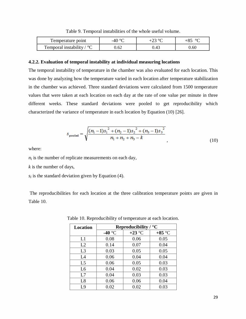
4.2.2. Evaluation of temporal instability at individual measuring locations

The temporal instability of temperature in the chamber was also evaluated for each location. This

was done by analyzing how the temperature varied in each location after temperature stabilization

in the chamber was achieved. Three standard deviations were calculated from 1500 temperature

values that were taken at each location on each day at the rate of one value per minute in three

different weeks. These standard deviations were pooled to get reproducibility which

characterized the variance of temperature in each location by Equation (10) [26].

, (10)

where:

ni is the number of replicate measurements on each day,

k is the number of days,

si is the standard deviation given by Equation (4).

The reproducibilities for each location at the three calibration temperature points are given in

Table 10.

Table 10. Reproducibility of temperature at each location.

Location Reproducibility / °C

-40 °C +23 °C +85 °C

L1 0.08 0.06 0.05

L2 0.14 0.07 0.04

L3 0.03 0.05 0.05

L4 0.06 0.04 0.04

L5 0.06 0.05 0.03

L6 0.04 0.02 0.03

L7 0.04 0.03 0.03

L8 0.06 0.06 0.04

L9 0.02 0.02 0.03

30

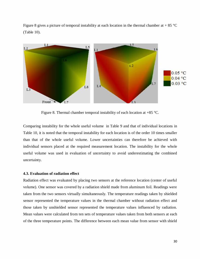
Figure 8 gives a picture of temporal instability at each location in the thermal chamber at + 85 °C

(Table 10).

Figure 8. Thermal chamber temporal instability of each location at +85 °C.

Comparing instability for the whole useful volume in Table 9 and that of individual locations in

Table 10, it is noted that the temporal instability for each location is of the order 10 times smaller

than that of the whole useful volume. Lower uncertainties can therefore be achieved with

individual sensors placed at the required measurement location. The instability for the whole

useful volume was used in evaluation of uncertainty to avoid underestimating the combined

uncertainty.

4.3. Evaluation of radiation effect

Radiation effect was evaluated by placing two sensors at the reference location (center of useful

volume). One sensor was covered by a radiation shield made from aluminum foil. Readings were

taken from the two sensors virtually simultaneously. The temperature readings taken by shielded

sensor represented the temperature values in the thermal chamber without radiation effect and

those taken by unshielded sensor represented the temperature values influenced by radiation.

Mean values were calculated from ten sets of temperature values taken from both sensors at each

of the three temperature points. The difference between each mean value from sensor with shield

31

and each value from sensor without shield was calculated. The radiation effect was evaluated by

the formula below [9]:

|δTradiation| ≤ Max|Tle-The| (11)

where

δTradiation is the radiation effect on temperature of the chamber,

Tle is the temperature of the sensor with low emissivity i.e. with radiation shield,

The is the temperature of the sensor with high emissivity i.e. without radiation shield.

The highest temperature difference between the temperature read by the unshielded and shielded

sensor from the three sets of measurements was considered to be the radiation effect. The

radiation effect results for the three temperature points are given in Table 11.

Table 11. Radiation effects.

Temperature point -40 °C +23 °C +85 °C

Radiation effect / °C 0.50 0.24 0.63

4.4. Evaluation of loading effect

In thermal ambient testing of space equipment, different kinds of equipment are tested at different

levels of satellite development. Individual circuit boards for specific purposes on the satellite and

other subassemblies are individually tested. Then the whole assembled payload is also tested.

These specimen give different loads to the thermal chamber that affect the chamber temperature

differently. It is required that the loads that are used in characterizing thermal chambers should be

similar to the loads that will be tested later in the characterized chamber [8]. In this study, the

loading effect on chamber temperature measurements was evaluated for three different loads: An

ESTCube-1 circuit board, an aluminum dummy for ESTCube-1 with four circuit boards in it and

an ESTCube-1 dummy with four circuit boards in an ESTCube-1 P-POD. These loads are typical

of the loads that will be tested in the thermal chamber using this method.

The DKD-R 5-7 [9] standard for calibration of thermal chambers states that the loading effect can

be evaluated by taking readings from the useful volume reference location (UVRL) in an empty

chamber and also in a loaded chamber. The loading effect can then be evaluated as the maximum

32

average difference between the two setups. In this study, this approach was not used because in

order to load the chamber with loads, the chamber door had to be opened and the metrological

conditions of the chamber in the empty chamber and the loaded chamber are not the same any

longer and cannot be compared to estimate the loading effect. An independent reference was

needed that does not get influenced by changed conditions.

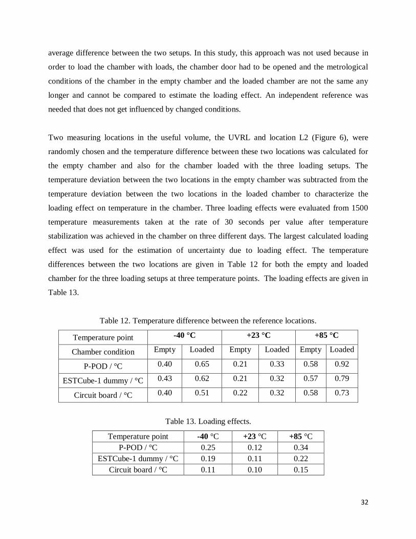
Two measuring locations in the useful volume, the UVRL and location L2 (Figure 6), were

randomly chosen and the temperature difference between these two locations was calculated for

the empty chamber and also for the chamber loaded with the three loading setups. The

temperature deviation between the two locations in the empty chamber was subtracted from the

temperature deviation between the two locations in the loaded chamber to characterize the

loading effect on temperature in the chamber. Three loading effects were evaluated from 1500

temperature measurements taken at the rate of 30 seconds per value after temperature

stabilization was achieved in the chamber on three different days. The largest calculated loading

effect was used for the estimation of uncertainty due to loading effect. The temperature

differences between the two locations are given in Table 12 for both the empty and loaded

chamber for the three loading setups at three temperature points. The loading effects are given in

Table 13.

Table 12. Temperature difference between the reference locations.

Temperature point -40 °C +23 °C +85 °C

Chamber condition Empty Loaded Empty Loaded Empty Loaded

P-POD / °C 0.40 0.65 0.21 0.33 0.58 0.92

ESTCube-1 dummy / °C 0.43 0.62 0.21 0.32 0.57 0.79

Circuit board / °C 0.40 0.51 0.22 0.32 0.58 0.73

Table 13. Loading effects.

Temperature point -40 °C +23 °C +85 °C

P-POD / °C 0.25 0.12 0.34

ESTCube-1 dummy / °C 0.19 0.11 0.22

Circuit board / °C 0.11 0.10 0.15

33

4.5. Estimation of measurement uncertainty for temperature of the chamber

4.5.1. Model equation

To get the actual temperature from the sensors in the chamber when doing measurements, the

following model was obtained.

TChamber = Tread Sensor + δTSensor + δTinh + δTinst + δTrad + δTload , (13)

where

TChamber is the temperature in the useful volume of the chamber,

Tread sensor is the temperature read from the sensor in the useful volume,

δTSensor is the deviation due to sensor calibration,

δTinh is the temperature deviation due to chamber temperature inhomogeneity,

δTinst is the temperature deviation due to chamber temperature instability,

δTrad is the temperature deviation due to chamber temperature radiation effect,

δTload is the temperature deviation due to loading effect.

4.5.2 Standard uncertainty of contributing components

All relevant contributions to uncertainties were taken into account and uncertainty budget was

estimated. Contributions to uncertainty included the combined standard uncertainty from

calibration of the sensors, spatial inhomogeneity, temporal instability, radiation effect, and

loading effect. For the loading effect, each loading setup was considered separately.

Equation (14) gives the formula used to calculate the uncertainty.

, (14)

where

uc(Tchamber) is the combined standard uncertainty of temperature in the useful volume of the

chamber,

uc (sensor) is the combined standard uncertainty from sensor calibration,

uinh is the uncertainty due to inhomogeneity,

uinst is the uncertainty due to instability,

urad is the uncertainty due to radiation effect,

uload is the uncertainty due to loading effect,

34

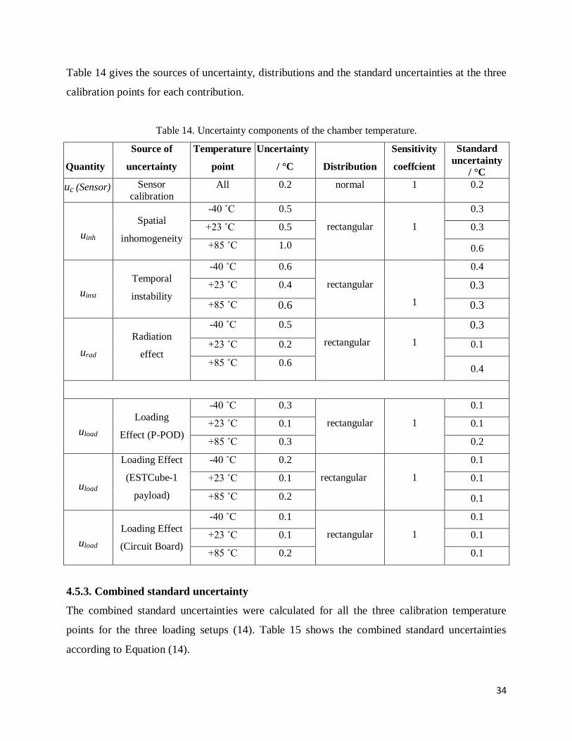
Table 14 gives the sources of uncertainty, distributions and the standard uncertainties at the three

calibration points for each contribution.

Table 14. Uncertainty components of the chamber temperature.

Quantity

Source of

uncertainty

Temperature

point

Uncertainty

/ °C

Distribution

Sensitivity

coeffcient

Standard

uncertainty

/ °C

uc (Sensor) Sensor

calibration All 0.2 normal 1 0.2

uinh

Spatial

inhomogeneity

-40 ˚C 0.5

rectangular

1

0.3

+23 ˚C 0.5 0.3

+85 ˚C 1.0 0.6

uinst

Temporal

instability

-40 ˚C 0.6

rectangular

1

0.4

+23 ˚C 0.4 0.3

+85 ˚C 0.6 0.3

urad

Radiation

effect

-40 ˚C 0.5

rectangular

1

0.3

+23 ˚C 0.2 0.1

+85 ˚C 0.6 0.4

uload

Loading

Effect (P-POD)

-40 ˚C 0.3

rectangular

1

0.1

+23 ˚C 0.1 0.1

+85 ˚C 0.3 0.2

uload

Loading Effect

(ESTCube-1

payload)

-40 ˚C 0.2

rectangular

1

0.1

+23 ˚C 0.1 0.1

+85 ˚C 0.2 0.1

uload

Loading Effect

(Circuit Board)

-40 ˚C 0.1

rectangular

1

0.1

+23 ˚C 0.1 0.1

+85 ˚C 0.2 0.1

4.5.3. Combined standard uncertainty

The combined standard uncertainties were calculated for all the three calibration temperature

points for the three loading setups (14). Table 15 shows the combined standard uncertainties

according to Equation (14).

35

Table 15. Combined standard uncertainties for three loading setups with coverage factor k=1.

Temperature point -40 ˚C +23 °C +85 ˚C

P-POD / °C 0.6 0.5 0.8

ESTCube-1 dummy / °C 0.6 0.5 0.8

Circuit board / °C 0.6 0.5 0.8

4.6. Evaluation of temperature reference point on test objects

A temperature reference point (TRP) is a point located on the test object which provides a

simplified representation of the unit temperature. Temperatures at the TRP are used to verify

requirements by analysis and test [28]. It is required that the same position on the test objects

where temperature values are taken when characterizing the thermal chamber is to be used when

testing equipment. A temperature reference point (TRP) must be selected on the unit external

surface and unambiguously identified in the respective mechanical interface control drawings

[29]. In this study, reference points were determined on all the three tests loads which shall also

be used as reference points for testing similar test objects. On the circuit board, the central

location on top of a chip (S5) was chosen as a TRP. This position was chosen because the

measurement of chip temperature is essential to the evaluation of thermal performance for the

design, application and manufacture of the module [30]. Also when the circuit boards are

switched on, the temperature of the chips is slightly higher than the temperature of all other

components on the circuit board. The temperature of chips on circuit boards is therefore of

uttermost importance.

On the P-POD and ESTCube-1 satellite dummy, experiments were carried out to determine the

TRP. It was still very crucial to monitor how the temperature affects the chips on the circuit

board while it is inside the payload. A sensor was mounted on the circuit board on the TRP and

the board was placed in the P-POD and dummy. Six sensors were mounted on the P-POD and

ESTCube-1 dummy, one sensor on each of their six surfaces. The setups were placed in the

chamber until temperature stabilization was achieved. Readings were taken from the sensors.

Table 16 gives the mean temperature values from the sensors at +85 °C with expanded

uncertainty at 95% confidence level with coverage factor k=2 as an example (Table 15).

36

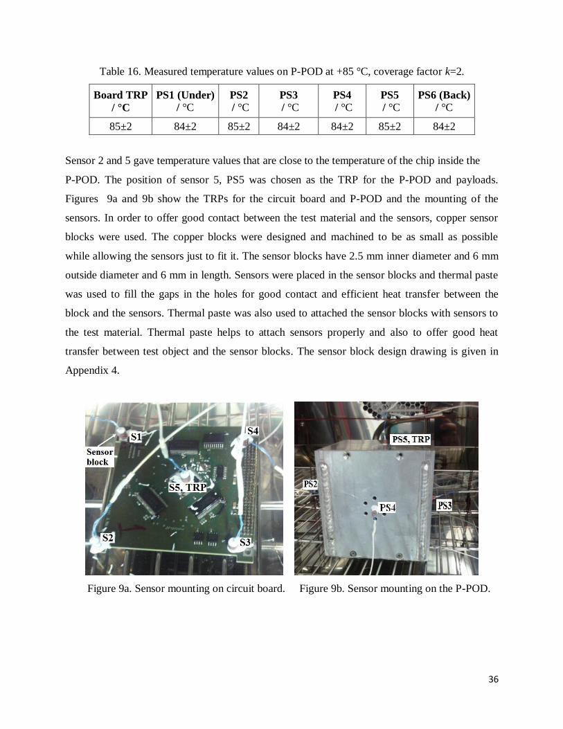
Table 16. Measured temperature values on P-POD at +85 °C, coverage factor k=2.

Board TRP

/ °C

PS1 (Under)

/ °C

PS2

/ °C

PS3

/ °C

PS4

/ °C

PS5

/ °C

PS6 (Back)

/ °C

85±2 84±2 85±2 84±2 84±2 85±2 84±2

Sensor 2 and 5 gave temperature values that are close to the temperature of the chip inside the

P-POD. The position of sensor 5, PS5 was chosen as the TRP for the P-POD and payloads.

Figures 9a and 9b show the TRPs for the circuit board and P-POD and the mounting of the

sensors. In order to offer good contact between the test material and the sensors, copper sensor

blocks were used. The copper blocks were designed and machined to be as small as possible

while allowing the sensors just to fit it. The sensor blocks have 2.5 mm inner diameter and 6 mm

outside diameter and 6 mm in length. Sensors were placed in the sensor blocks and thermal paste

was used to fill the gaps in the holes for good contact and efficient heat transfer between the

block and the sensors. Thermal paste was also used to attached the sensor blocks with sensors to

the test material. Thermal paste helps to attach sensors properly and also to offer good heat

transfer between test object and the sensor blocks. The sensor block design drawing is given in

Appendix 4.

Figure 9a. Sensor mounting on circuit board. Figure 9b. Sensor mounting on the P-POD.

37

4.7. Evaluation of rate of temperature change in the thermal chamber

It was noted (Table 14) that among inhomogeneity, instability, radiation effect and loading effect,

the smallest component contributing to uncertainty was the loading effect. However, loading was

observed to affect the rate of temperature change in the chamber. The rate of temperature change

in the chamber was investigated with an empty chamber and a chamber loaded with the three

loading setups which are typical of space equipment that are tested in thermal chamber at

different levels of satellite development. The items included an ESTCube-1 size circuit board, an

ESTCube-1 payload dummy with four circuit boards in it and the complete ESTCube-1 payload

in protective P-POD. The temperature of these materials was cycled starting from -40 °C to +85

°C and from +85 °C to -40 °C. Figure 10 show the effect of loading on the rate of change of

temperature with the ESTCube-1 dummy and the four circuit boards in the protective P-POD.

Figure 10. Rate of change of temperature with P-POD load.

The rate of temperature change in the chamber was slower with loaded chamber setup. The rate

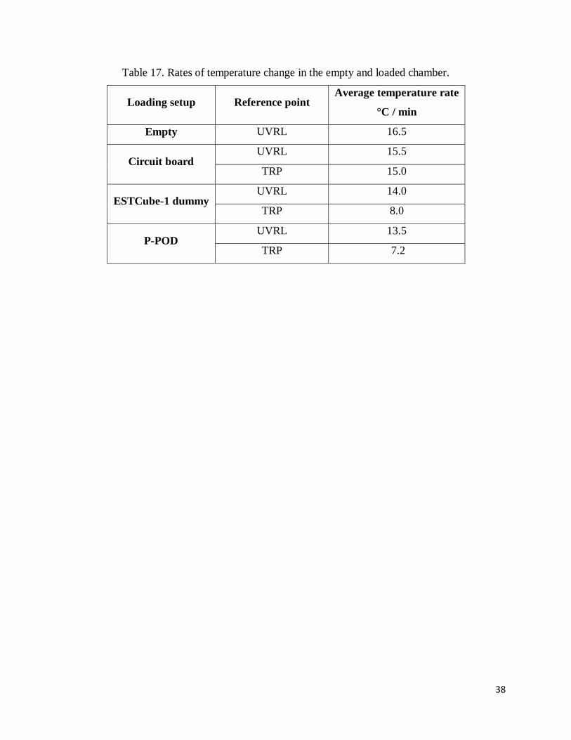
of temperature change was noted to be even slower on the surface of the test object. Table 17

gives the average rate of temperature change in an empty chamber and in the loaded chamber at

the UVRP and in loaded chamber on the test object TRP of each of the three loading setups.

38

Table 17. Rates of temperature change in the empty and loaded chamber.

Loading setup Reference point Average temperature rate

°C / min

Empty UVRL 16.5

Circuit board UVRL 15.5

TRP 15.0

ESTCube-1 dummy UVRL 14.0

TRP 8.0

P-POD UVRL 13.5

TRP .7.2

39

5. Thermal ambient test of sample space technology equipment

In the second part of this study, the characterized thermal chamber was used for thermal ambient

testing of a sample space technology equipment.

5.1. Test specimen

An ESTCube-1 satellite non-flight command and data handling system (CDHS) board was used

as a test object. The CDHS has a crucial role in a satellite mission. It has a microprocessor that is

used for coordinating the satellite and for logging and storing of data on three flash memory

devices mounted on the board. It also has sensors that are used for altitude determination of the

satellite [31-33]. Figure 11, shows the CDHS board in the chamber during the tests.

Figure 11. CDHS board in a thermal chamber during tests.

5.2. Summary of the thermal ambient test

Thermistor temperature sensor was mounted onto the specimen on the TRP (microprocessor

chip) and the temperature of the test object during the test cycles was recorded in time using

Labview software to track the actual temperature of the specimen. A test program with four

cycles that was developed using S!mpati software was used in the test (Figure 5). In order to

maintain good contact between the test material and the sensor, copper sensor block and thermal

paste were used as described in section 4.6. The equipment was placed in the useful volume of

the chamber on an insulating material to ensure that the board does not touch the metal surface of

the chamber shelf which could short circuit the board. The USB data cable for powering the

40

board and for data logging from it together with sensor cable were passed through the cable hole

on the side of the chamber and the cover was properly replaced. The door of the chamber was

properly closed.

5.3. Initial functional test

The specimen was visually examined and functional tests were carried out before starting thermal

cycling. The performance of the specimen was recorded. The board was able to communicate

with the computer apart from the fact that one of the three flash memory devices was not

functioning.

5.4. Thermal cycling

The specimen was thermal cycled with 4 cycles spanning in the extreme temperatures of -40 °C

as the minimum extreme temperature and +85 °C as the maximum extreme temperature. The

specimen was exposed to dwell times of 2 hours at each extreme temperature.

5.5. Functional tests during and at the end of thermal cycling

The specimen was tested for cold start at the minimum extreme temperature in the first cycle

after a dwell time of two hours to check for cold start capability and then it was allowed to run

during the ramp up to higher extreme temperature where it was powered off and on again to

check for hot start capability. During both cold start and hot start tests, the specimen was able to

power up. During thermal cycling it was observed that the CDHS had done several resets. During

the period of resets, communication with the computer was lost. Unplanned resets have also been

observed on the actual ESTCube-1 satellite that is now in space. The reason for the resets was

discovered to be a software problem. Functional and performance tests were also performed at

the end of the thermal ambient test. The test object was functioning well and was able to

communicate with the computer at the end of all the four cycles. The test was repeated two times

and the results were reproducible apart from the fact that the second flash memory device out of

the two working devices was noted to have stopped working. Figure 12a, shows the temperature

measured by the sensor on the TRP of the test object, the set profile and the difference of the two.

The figure also shows the time when the functional test were performed.

41

Figure 12b shows the required temperature margins (±5 °C) by the standard [10] and the

uncertainty region. The uncertainty is presented as expanded uncertainty at 95% confidence level

with coverage factor k=2 (Table 15).

Figure 12a. CDHS thermal cycling.

Figure 12b. Uncertainty and required limits.

42

6. Conclusions

A method for thermal ambient tests of space equipment has been developed in this study.

Sensors were installed in the thermal chamber and a Labview software for data acquisition

using a data logger was developed. The thermal chamber at Tartu Observatory was

characterized. Different sources of uncertainty were investigated and uncertainty budget for

the chamber was established for specific loads that are tested at different levels of satellite

development. A sample space technology equipment was tested using the method in the

thermal chamber. The method achieves expanded measurement uncertainty of ±2 °C for the

temperature measurement range (-40...+85) °C at 95% confidence level, k=2. The uncertainty

achieved by the method complies with the requirements for testing space equipment in thermal

ambient testing. However the uncertainty can further be improved. The major contributing

components to the combined standard uncertainty for this method are spatial inhomogeneity

and temporal instability. Uncertainty can therefore be reduced if further studies are done to

investigate the causes and solutions for improvement of these parameters.

43

A Method for Thermal Ambient Tests of Space Technology Equipment in a Thermal chamber –

Development and Validation

Sinai Mwagomba

Summary

Thermal ambient test is one of the series of analyses that are carried out on equipment to be

launched in space in order to check their capability to withstand the environmental conditions to

be encountered in orbit while maintaining the desired performance. It is also one of the

requirements to be fulfilled for the space technology facility to be qualified and accepted for

launching. The aim of this work was to develop a method for thermal ambient testing of space

equipment at Tartu Observatory, to validate it and come up with an uncertainty budget.

A commercial Weisstechnik WKL 64 thermal chamber in Tartu Observatory was used in the

task to simulate the temperature environment that satellites encounter in space. The system for

the method was developed. Temperature sensors were installed in the chamber and were

connected to the computer via a data logger for registering temperature readings. A software for

data logging was developed and implemented.

The uncertainty sources of temperature readings in the chamber were validated and the

uncertainty budget for the method was evaluated. The method achieves expanded measurement

uncertainty of ±2 °C in the temperature measurement range (-40…+85) °C at 95% confidence

level, k=2. The achieved uncertainty level complies with the requirements for testing space

equipment in thermal ambient tests. The method was applied for testing of actual space

equipment at different chamber loading setups.

44

8. List of references

[1] A. Globus, J. Crawford, J. Lohn and A. Pryor, “Scheduling Earth Observing Satellites with

Evolutionary Algorithms,” In Conference on Space Mission Challenges for Information

Technology (SMC-IT), (2003).

[2] N.L. Johnson, "Medium Earth Orbits: is there a need for a third protected region?," 61st

International Astronautical Congress. Prague, CZ, (2010).

[3] L. Jacques, “Thermal Design of the Oufti-1 nanosatellite,” Master Thesis in Aerospace Engi-

neering, University of Liège, (2009).

[4] Pumpkin, Inc., CubeSat Kit User Manual,” San Francisco, USA, (2005).

[5] ALMA Space, European Student Earth Orbiter Satellite, Experiment interface document, Part

A (E1D-A), (2013).

[6] J.A. Angelo, Encyclopedia of Space and Astronomy, Facts on the file Science library, New

York, (2006)

[7] J. A. Angelo, Satellites (Facts on the file Science Library, New York, 2006).

[8] M. L. DONA, “Methods of Calibration and characterization of Temperature Controlled

Environments,” U.P.B. Sci. Bull., Series C, Vol.72, Iss. 2, 197-210, (2010).

[9] Deutscher Kalibrierdienst (DKD), Calibration of Climatic Chambers, ed 7, DKD

Braunschweig, (2009).

[10] ECSS Secretariat, Space Engineering Testing, ESA-ESTEC, Requirements & Standards

Division, Noordwijk, Netherlands, (2012).

[11] Joint Committee for Guides in Metrology, JCGM 100:2008, “Evaluation of measurement

data - guide to the expression of uncertainty in measurement,” JCGM, (2008).

[12] T. Al-Hawari, S. Al-Bo'ol, and A. Momani, “Selection of Temperature Measuring Sensors

Using the Analytic Hierarchy Process,” JJMIE, Vol. 5, 451-459, (2011).

[13] ALCATEL Space, Payload verification and test requirements, Proteus Unser’s Manual

document (PRO. LB. O. 003. ASC), chap 6, (2003).

[14] W. M. Foster II, “Thermal Verification Testing of Commercial Printed-Circuit Boards for

Space flight,” NASA Technical Memorandum 105261, presented at Annual Reliability and Main-

tainability Symposium sponsored by the Institute of Electrical and Electronics Engineers, Las

Vegas, Nevada, January 21-23, (1992).

45

[15] BIPM, “International vocabulary of metrology – Basic and general concepts and associated

terms (VIM),” (2008).

[16] NASA, Hardware Requirements Document for the Human Research Facility, Rack 2

Workstation (R2WS), (2000).

[17] EVS-EN 60068-2-14, Environmental testing, Change of temperature, Part 2-14, (2009).

[18] Installation and Operation manual, Simpati software Version 4.06, (2011).

[19] Weiss Technik, Temperature and Climatic Test Chambers, Greizer, Germany, (2010).

[20] Measurement Computing Corporation (MCC), USB Temp Multi-sensor Temperature

Measurement User guide, rev 13, Massachusetts, USA (2014).

[21] Siemens Matsushita Components, Temperature Measurement Miniature Sensors data sheet

B57861, (2006).

[22] Nexus, 50VMTX Miniature PTFE coaxial cable data sheet, Iss. 2, Draveil, France, (1999).

[23] M. Jiménez, R. Palomera, and I. Couvertie, “Analog Signal Chain,” in Introduction to

Embedded Systems using Microcontrollers and the MSP430, (University of Puerto Rico,

Mayagüez, Puerto Rico), pp. 537-595, (2014).

[24] Automatic Systems Laboratories (ASL), F100 Precision thermometer user manual,

Brentwood, N. America, (2011).

[25] FLUKE Corporation, 287/289 True RMS Digital multimeters User manual, Rev 1 7/08,

Eindhoven, Netherland, (2007).

[26] D.L. Massart, B.G.M. Vandeginste, L.M.C. Buydens, S. De Jong, P.J. Lewi, and J. Smeyers,

Data Handling in Science and Technology, Handbook of Chemometrics and Qualimetrics part A,

Elsevier Science B.V., Amsterdam, (1997).

[27] DIN 50011-12, “Artificial climates in technical applications; air temperature as a

climatological quantity in controlled-atmosphere test installations,” (2009).

[28] EADS astrium, “General Design and Interface Requirements,” Iss 3.1, UK, (2010).

[29] ECSS Secretariat, Space Engineering Thermal Control, ESA-ESTEC, Requirements &

Standards Division, Noordwijk, Netherlands, (2012).

[30] J. Yin, “High Temperature SiC Embedded Chip Module (ECM) with Double-Sided

Metallization Structure,” Doctoral Thesis, Virginia Polytechnic Institute and State

University, (2005).

46

[31] I. Sünter, “Software for the ESTCube-1 command and data handling system, ” Masters The-

sis, University of Tartu, (2014).

[32] S. de Jong, G.T. Aalbers and J. Bouwmeester, “Improved command and data handling sys-

tem for the delfi-n3xt nanosatellite,” in 59th

International Astronautical Congress, Glasgow,

Scotland, UK, (2008).

[33] J.R. Wertz and W.J. Larso, Space mission analysis and design, 3rd ed., Microcosm Press, El

Segundo, California, (1999).

47

Meetod kosmosetehnoloogia seadmete katsetamiseks temperatuurikeskkonnas – väljatöötamine

ja valideerimine

Sinai Mwagomba

Kokkuvõte

Temperatuurikeskkonna katse on üks nendest uuringutest, mida tehakse kosmosesse saadetavate

seadmete puhul kontrollimaks nende võimet vastu pidada orbiidil valitsevatele keskkonna-

tingimustele. See on ühtlasi üks kohustuslikest katsetest, mille alusel kvalifitseeritakse seade

kosmosekõlbulikuks. Käesoleva töö eesmärgiks on Tartu Observatooriumis kosmosetehnoloogia

seadmete temperatuurikeskkonna katseteks vajaliku metoodika väljatöötamine, selle

valideerimine ning mõõtemääramatuste allikate osakaalu hindamine.

Tartu Observatooriumis kasutatakse temperatuurikatsetel kosmoses valitsevate tingimuste

simuleerimiseks tööstuslikku termokambrit WKL-64, mille täienduseks ehitati temperatuuri-

anduritest ja arvutiühendusega andmehõiveseadmest koosnev mõõtesüsteem. Andmehõiveks

arendati ja rakendati spetsiaalne tarkvara.

Kambris tehtavate temperatuurimõõtmiste jaoks hinnati mõõtemääramatuse allikaid ning meetodi

rakendamiseks koostati mõõtemääramatuse koondtabel. Meetod võimaldab temperatuuri

laiendmääramatust ±2 °C mõõtepiirkonnas (-40…+85) °C usaldusnivool 95% (kattetegur k=2).

Saavutatud mõõtemääramatuse tase vastab kosmoseaparatuuri temperatuurikatsetele esitatud

nõuetele. Meetodit rakendati kosmoseaparatuuri katsetamiseks temperatuurikambri erinevate

täitemahtude puhul.

48

9. Acknowledgements

First of all I would like to thank my supervisors Ph.D. Riho Vendt and Professor Ivo Leito for

all the support, advice and guidance throught the duration of doing my thesis.

Secondly I would like to thank Kaspars Laizans for all the help he offered to acquire the

required materials used in the task.

Thirdly I would like to thank Indrek Sünter for the help he offered to do functional test of

CDHS during thermal ambient tests.

I would also like to thank Tartu Obsevatory for allowing me to do my research there.

I would also like to thank all the ESTCube-1 team members for all the support rendered.

Last but not least I would like thank Astrid Pung for helping with proof reading the thesis and

translating the summary of this thesis into Estonian language.

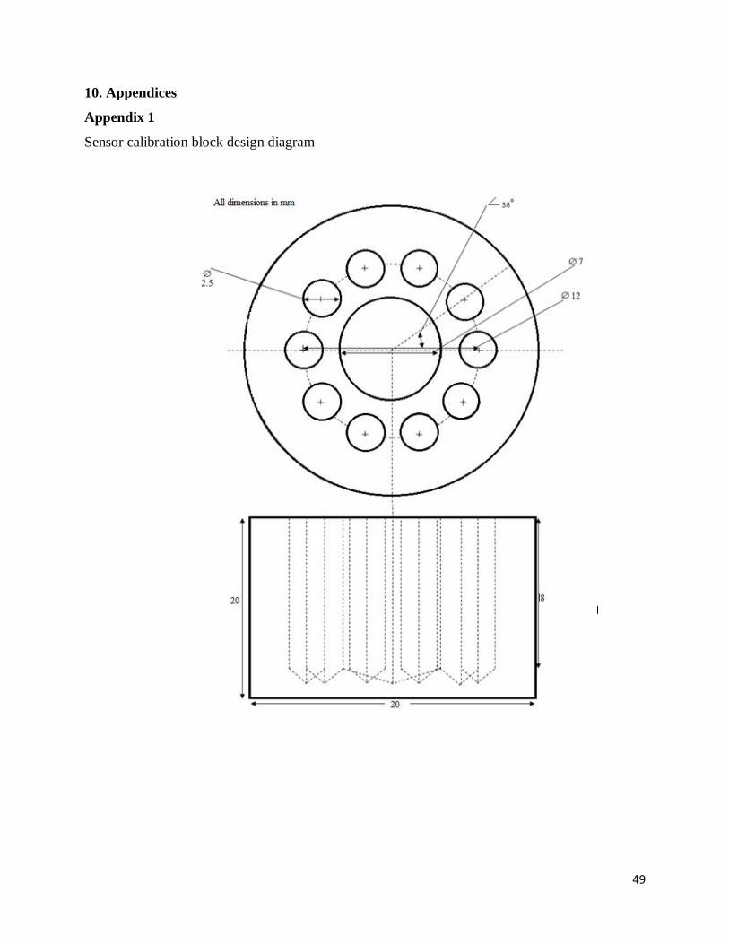
49

10. Appendices

Appendix 1

Sensor calibration block design diagram

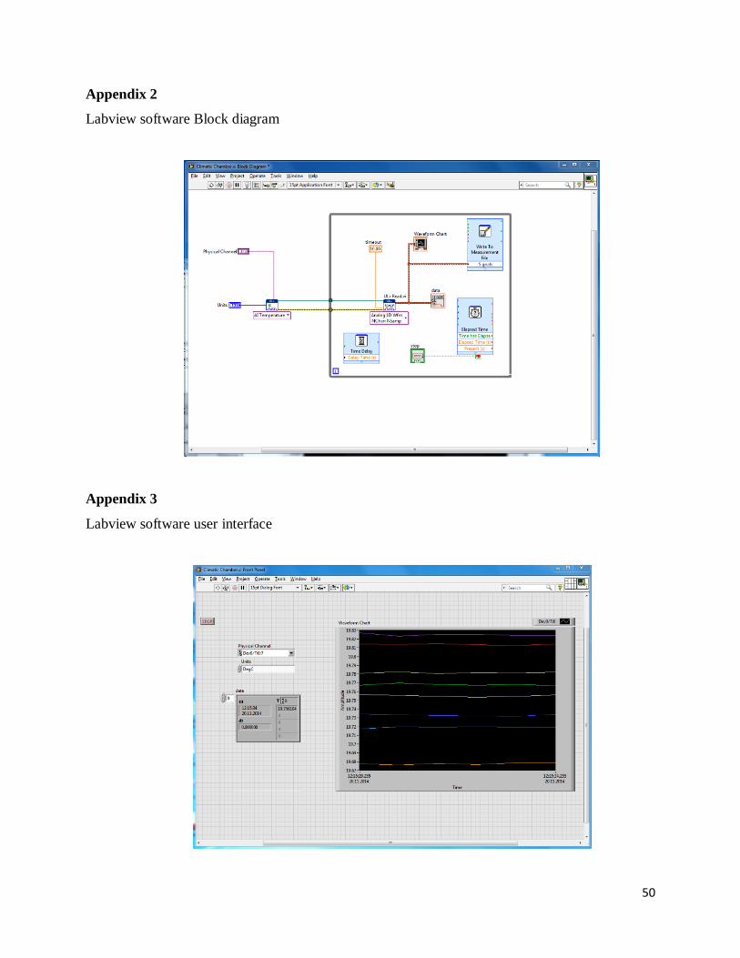
50

Appendix 2

Labview software Block diagram

Appendix 3

Labview software user interface

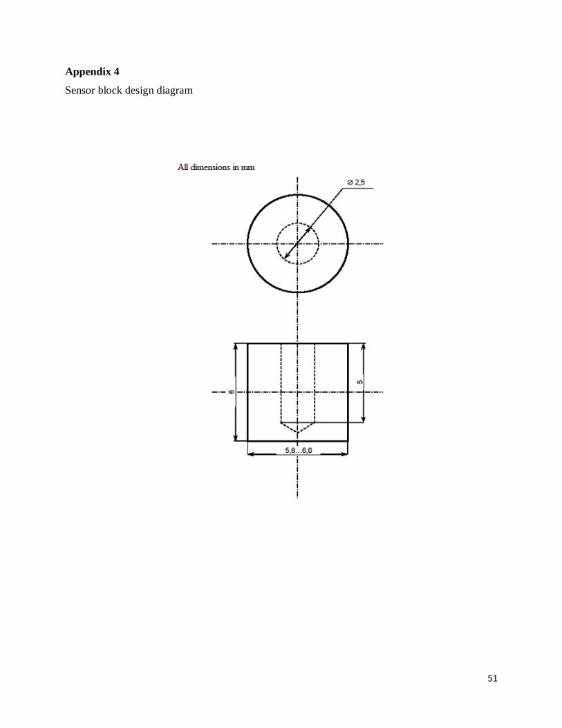
51

Appendix 4

Sensor block design diagram

52

Non-exclusive license to reproduce thesis and make thesis public

I, Sinai Mwagomba, (date of birth: 23.11.1983.),

1. herewith grant the University of Tartu a free permit (non-exclusive license) to:

1.1. reproduce, for the purpose of preservation and making available to the public, including

for addition to the DSpace digital archives until expiry of the term of validity of the copyright,

and

1.2. make available to the public via the university's web environment, including via the

DSpace digital archives, as of 19.12.2014 until expiry of the term of validity of the copyright,

“A method for thermal ambient tests of space equipment - developement and validation”

(title of thesis)

supervised by PhD Riho Vendt and Professor Ivo Leito.

2. I am aware of the fact that the author retains these rights.

3. This is to certify that granting the non-exclusive license does not infringe the intellectual

property rights or rights arising from the Personal Data Protection Act.

Tartu 11.12.2014