1

A goal programming model for the analysis of a frozen

concentrated orange juice production and distribution system

José Renato Munhoz Citrovita Agro Industrial Co., Brazil

(renato.munhoz@citrovita.com.br)

Reinaldo Morabito Production Engineering Department

Universidade Federal de São Carlos

13565-905 São Carlos, SP, Brazil

(morabito@power.ufscar.br)

Abstract: In this work we propose a model based on linear and goal programming to

support decisions in the blending process and distribution of frozen concentrated orange

juice. The model explores the importance of blending decisions for the logistic analysis

of the orange juice distribution, besides transportation and storage decisions. It utilises

well-known concepts from the literature of blending problems and multistage,

multiproduct and multiperiod production planning problems. A case study was

developed in an orange juice company located in São Paulo State, Brazil, and the

preliminary results are promising.

Keywords: Goal programming, logistics of distribution, production planning, frozen

concentrated orange juice.

1. Introduction

In the Brazilian orange juice industry the production and distribution of frozen

concentrated orange juice (FCOJ) involves the analysis of a large amount of information

in order to optimise the usage of available resources. The co-ordination of production,

2

inventory and transportation of raw materials (different orange varieties), intermediary

products (concentrated juice of each orange variety, namely base) and final products

(FCOJ obtained by blending different bases) is particularly important because of the

combination of the seasonality of the fruits and the relative regularity of the product

demands. Brazil is the largest world producer and exporter of FCOJ (FAO [3][4]) and,

for certain companies in this country, small improvements in their production and

distribution systems can result in substantial savings.

In this study we present a model based on linear and goal programming to

support tactical and operational decisions in the process of blending bases for the

production of FCOJ, as well as transportation and storage of the products. We explore

the importance of blending decisions for the logistics of the FCOJ distribution. The

model was inspired by a case study developed in an orange juice company located in

São Paulo State that exports their products basically to United States, Europe and Japan,

and the shipments are limited by periodic vessel schedules. The priority goals of the

model are to minimise blending and distribution costs, the later tends to maximise the

utilisation of bulk systems rather than transporting and storing products in drums, since

they are more economic (Pinto [9]). Other goals are to minimise the product quality

deviations from certain targeted specifications. Such optimisations are presently

performed in the company by means of simulations on spreadsheet software.

The proposed model utilises well-known concepts from the literature of blending

problems and multistage, multiproduct and multiperiod production planning problems

(e.g., Johnson and Montgomery [6], Hax and Candea [5], Shapiro [10], Nahmias [8]). It

aims to support medium to short term decisions such as: how much of each product to

produce in each period, and how (in bulk or drums) and where to move and store the

products, taking into account capacity constraints, demands and the vessel shipment

schedule. This way, the model also considers blending decisions such as how much of

each base to utilise for the composition of each product (since a product may be

produced by different mix of bases). Moreover, the model considers storing and

transporting products in drums as soon as the capacity of bulk systems becomes a

limitation. To solve the model, we utilise the modelling language GAMS (General

Algebraic Modelling System) and the solver GAMS/MINOS (Brooke et al [2]). In spite

of being based on a particular case study, we believe that the model is sufficiently

generic or can be easily extended for application to other orange juice companies.

3

The paper is organised as follows: the next section presents a brief description of

the FCOJ production process and details the problem under consideration. Section 3

proposes a linear and goal programming model for the problem, and section 4 analyses

some computational results obtained by applying the model to a simplified situation of

the case study (because of unavailability of data and in order to protect interests of the

company). Finally, section 5 presents concluding remarks and discusses some

perspectives for future research.

2. Problem definition

The development of the orange juice industry took place in the United States in

the 30's due to the increase of orange juice consumption (Viegas et al [11]). At that time

campaigns were diffused stimulating the substitution of the fruit (the mean daily

consumption was half fruit per person) by the juice (a glass of juice uses three to four

fruits). At the end of the decade more than 90% of the American families were daily

consumers of orange juice. In Brazil the industrial production of orange juice began only

in the 60's but since 1966 the country has had the world leadership in production and

exportation of FCOJ. Table 1 presents some terminology utilised in the orange juice

industry; the main characteristics of oranges are the brix, ratio and variety. In the

following we briefly describe a typical production process of FCOJ.

Oranges of different varieties are transported to the plant by trucks, which are

unloaded by hydraulic ramps. The oranges are carried by conveyor belts and elevators

until storage bins. Based on the characteristics of the fruits, they follow to washing,

grading and classifying processes, and then to the extraction room. In this local

extractors separate the fruits into three parts: juice, peel, and oil and aqueous solution

with small particles of peel. The juice is pumped to multiple-stage evaporators and,

while being concentrated, two other by-products are produced: oil phase and water

phase. The concentrated juice is then frozen and stored in bulk in tank farms. These

intermediary products called bases are then mixed, according to the "blending plan"

(defined below), in order to produce the ordered FCOJ. The main differences between

two final products are their specifications of ratio and orange variety. The FCOJ is

stored in bulk in tank farms, or is placed in drums of 200 litres and stored in refrigerated

warehouses (cold storage).

4

Figure 1 depicts the "basic (annual) plan of the season", which relates the

"blending plan" of bases to the "sales plan" of FCOJ, the "initial inventories" of bases

and FCOJ (in the beginning of the season), the "fruit plan" (procurement of oranges), the

"extraction plan" (production of bases) and the "distribution plan" (transportation and

storage of FCOJ). Note that the basic plan of the season involves the co-ordination of

different departments of the company, such as procurement (of fruits), sales (of FCOJ),

production, logistics and quality, in order to optimise the usage of available resources.

Basically the blending plan determines how much and when to blend the different bases

of the tank farms in order to produce the ordered FCOJ. These bases are obtained

according to the fruit and extraction plans in such a way as to satisfy the sales and

distribution (e.g., vessel shipment schedule) plans.

As mentioned in section 1, in this study we are concerned with the decisions in

the blending process of bases to produce FCOJ, and in the distribution (transportation

and storage) system of FCOJ. Figure 2 schemes the situation in a network flow: from

left to right, the first node represents inventories of bases in the tank farms (in bulk) of

the plant, the next two nodes represent inventories of FCOJ in the tank farms (in bulk)

and cold storage (in drums) of the plant, respectively, and the last two nodes represent

inventories of FCOJ in the external tank farms (in bulk) and cold storage (in drums),

respectively, available for the vessel shipment. The arcs between nodes correspond to

the flows (blending or transportation) of bases and products (in bulk or drums) for each

period (e.g., a week) of the planning horizon (e.g., part or the whole duration of the

season). Note that in the cases of product transportation from the plant tank farms (in

bulk) to the external cold storage (drums), or from the plant cold storage (drums) to the

external tank farms (in bulk), transportation includes the operation of packaging or

unpackaging the product, respectively.

For the purpose of this study, the fruit, extraction and sales plans (figure 1), as

well as the vessel shipment schedule in the distribution plan, are assumed to be known.

A question is to determine the quantities and periods of the planning horizon that the

bases are mixed to produce the demanded products. Another question is to choose the

product form (in bulk or packaged in drums) and warehousing places (plant or external

tank farms and cold storage) so that total costs are minimised. These costs are composed

by blending, transportation and warehousing costs, plus financing costs of anticipating

the blending of bases and transportation of products with respect to their periods of

5

demand. Warehousing costs do not include capital (opportunity) costs given that these

are considered in the financing costs. For simplicity, the model of next section considers

only one plant and only one location for the external warehouses (external tank farms

and cold storage), since in the case study these warehouses are located very close to the

seaport. The model can be easily extended to deal with situations involving different

plants and warehouses with different locations and operational costs.

3. Mathematical modelling

As mentioned above, the mathematical formulation utilises well-known concepts

of the literature of blending problems and multistage, multiproduct and multiperiod

production planning problems; see, e.g., Johnson and Montgomery [6], Williams [12],

Shapiro [10] and Nahmias [8]. Product quality specifications, capacity limitations of

blending and storing bases and products, and material balancing are the main constraints

of the model; the last one being responsible for the link between different planning

periods and locations.

Tables 2 and 3 define the variables and parameters utilised in the formulation (all

variables and parameters are non-negative). The indices j, p, k, l and t are associated as

follows: j represents the type of base (hamlin, BR10, ...), p represents the type of

product (PA11, PA12, ...), k represents the form of the inventory of the plant (bulk,

drum), l represents the form of the inventory of the external warehouse (bulk, drum),

and t represents the period (1, 2, ... weeks). Without loss of generality, some parameters

are supposed to be constant along the planning horizon.

The objective function F to be minimised is the sum of the costs of:

•

blending: ∑∑∑∑t k j p

kjpt

kj xbcb

•

transportation: ∑∑∑∑t k l p

klpt

klp xtct

•

warehousing: ∑∑ ∑∑∑ ∑∑∑++t j t k p t l p

lpt

lp

kpt

kpjtj epehpeepfhpfebhb

•

financing: ( )∑ ∑∑∑∑∑ ++t t l p

lpt

lp

k p

kpt

kpt

k epetxtepeepftxb

6

Note in the expression above that ( )kpt

kpt

k epeepftxb + is the opportunity cost of

the inventory of product p in the plant and external warehouses in form k in period t.

This is the cost of anticipating the blending for the production of this product in one

period. Similarly, lpt

lpepetxt is the cost of anticipating the transportation of product p to

the external warehouse in form l in one period, with respect to its required demand.

Therefore, the objective function of the model is:

Min F =∑∑∑∑t k j p

kjpt

kj xbcb + ∑∑∑∑

t k l p

klpt

klp xtct +

∑∑ ∑∑∑ ∑∑∑++t j t k p t l p

lpt

lp

kpt

kpjtj epehpeepfhpfebhb +

( )∑ ∑∑∑∑∑ ++t t l p

lpt

lp

k p

kpt

kpt

k epetxtepeepftxb (1)

The constraints of the model refer to material balancing, limits for product ratios,

inclusion of base hamlin in the mix, and capacities of blending and warehousing.

•

Constraints of material balancing for each period, product/base and form:

∑∑−+= −k p

kjptjttjjt xbprebeb 1, ∀ j, t (2)

∑ ∑−+= −j l

klpt

kjpt

ktp

kpt xtxbepfepf 1, ∀ k, p, t (3)

∑ −+= −k

lpt

klpt

ltp

lpt dxtepeepe 1, ∀ l, p, t (4)

•

Constraints for the ratio of each product, form and period:

( )∑∑ +≤j

kjpt

jp

kjptj xbratpxbratb 8.0 ∀ k, p, t (5)

∑ ∑≥j j

kjptp

kjptj xbratpxbratb ∀ k, p, t (6)

Equations (5)-(6) are typical of blending problems and define the acceptable

interval [ ]8.0, +pb ratbratp for the ratio of product p.

•

Constraints for adding base hamlin to each product, form and period:

7

∑=j

kjptt

kpthamlin xbpercxb ,"" ∀ k, p, t (7)

Equation (7) is also a blending constraint and specifies the percentage tperc of

base hamlin to be added to the mix of product p in each period t.

•

Constraints of capacity of blending in each period:

∑∑∑ ≤k j p

tkjpt bxb ∀ t (8)

•

Constraints of capacity of the plant and external warehouses in each period:

∑ ∑ ≤+j p

bulkbulkptjt abepfeb """" ∀ t (9)

∑ ≤p

drumdrumpt abepf """" ∀ t (10)

∑ ≤p

llpt atepe ∀ l, t (11)

The linear programming model (1)-(11), together with the non-negativity

constraints of the variables, was coded in the modelling language GAMS and solved in

a microcomputer by the solver GAMS/MINOS (Brooke et al [2]). It is worth mentioning

that this model can be easily adapted to treat situations where the costs are convex

(approximating them by piecewise linear functions; see e.g. Bazaraa et al [1]).

A goal programming approach

Goal programming is a simple modification and extension of linear

programming which allows a simultaneous solution of a system of complex objectives

rather than a single objective (Hax and Candea [5]). It can be applied when different

objectives appear explicitly and the trade-off among them should be analysed based on a

set of priorities. To formulate a goal programming model one has to specify a set of

goals along with the priority level associated with each of them. In particular, a decision

maker may not be able to determine precisely the relative importance of the goals. When

this is the case, preemptive goal programming may prove to be a useful tool (Winston

[13]).

8

In the present blending process, the managerial decisions may involve other

objectives rather than minimising costs, for instance, the product ratios should be as

close as possible to the middle of the acceptable ratio interval. For example, if a product

has minimum and maximum ratio specifications 14 and 14.8, it is desired that its ratio

yields as close as possible to 14.4. This situation can be dealt with achieving the

following two goals:

•

Goal 1, with top priority, is to minimise the sum of the costs of blending,

transportation, warehousing and financing (equation (1)) or, equivalently, minimise

the deviation of these costs from the objective "zero cost".

•

Goal 2, of secondary priority, is to minimise the deviation of the product ratio from

the objective "mean ratio".

Using the deviation variables of table 4, we define a new objective function for

model (1)-(12) given by:

++ ∑∑∑

−++

t k p

kpt

kptp sscPsP )()(min 22211 (12)

where P1>>P2 and pc is the relative weight of each product p (in the present study we

used 1=pc ). The constraints (2)-(11) continue valid and it is necessary to add the

following constraints of goals 1 and 2 to the model:

•

Constraint of goal 1 obtained from equation (1):

∑∑∑∑t k j p

kjpt

kj xbcb + ∑∑∑∑

t k l p

klpt

klp xtct +

∑∑ ∑∑∑ ∑∑∑++t j t k p t l p

lpt

lp

kpt

kpjtj epehpeepfhpfebhb +

( )∑ ∑∑∑∑∑ ++t t l p

lpt

lp

k p

kpt

kpt

k epetxtepeepftxb - 01 =+s (13)

•

Constraint of goal 2 obtained from equations (5)-(6):

( )∑∑ +=+− −+

j

kjpt

jp

kpt

kpt

kjptj xbratpssxbratb 4.022 ∀ k, p, t (14)

Note that constraint (13), together with the new objective function (12),

establishes that the total costs of blending, transporting, warehousing and financing

9

should be as close as possible to zero. Similarly, constraint (14) with the objective

function (12) establishes that the ratio of product p, obtained by blending different bases

j in each period t, should be as close as possible to the middle of the acceptable interval

specified for this product )4.0( +pratp .

The preemptive goal programming (2)-(14), together with non-negativity

constraints of the variables, was also coded in the modelling language GAMS and

solved in a microcomputer by the solver GAMS/MINOS, as discussed in next section.

Initially model (2)-(14) was solved minimising the deviation of goal 1 (zero cost), that

is, simply ignoring goal 2 of objective function (12) in order to obtain the minimum cost *F . Then model (2)-(14) was solved minimising the deviation of goal 2 (mean ratio)

under goal 1, that is, ignoring goal 1 of objective function (12) and adding to the model

the minimum cost constraint: *1 Fs =+ .

4. Computation experiments

As mentioned in section 3, the linear models (1)-(11) and (2)-(14) were coded in

the modelling language GAMS and solved by GAMS/MINOS, a solver written in

Fortran for the analysis of linear and non-linear programs (Brooke et al [2]).

GAMS/MINOS solves linear programs utilising a primal simplex algorithm (Bazaraa et

al [1]). For more details of the model implementations and the solutions obtained, the

reader can consult Munhoz [7].

The analysis of model (1)-(11) was performed on a simplification of the real

problem due to data unavailability and to protect interests of the company. The number

of periods, bases and final products were reduced from 51 to 5, 8 to 4 and 7 to 3,

respectively, regarding to the actual situation. This way, the total number of variables

and constraints decreased from 8976 to 260 and 4233 to 195, respectively. It is worth

mentioning that the typical sizes of the linear model in practical situations are not a

limitation for the methodology used (modelling language GAMS with solver

GAMS/MINOS).

Different scenarios were investigated perturbing parameters and changing the

capacities of blending and warehousing in order to evaluate the performance of the

model. The detailed input data utilised in each scenario can be found in Munhoz [7].

10

Tables 5-7 present a resume of the results for four scenarios briefly discussed below

(these solutions were obtained in a few seconds by the solver GAMS/MINOS using a

Pentium microcomputer).

Scenario 1

Some of the input parameters utilised in scenario 1 are: t = (1, ..., 5), tperc =

(10, 10, 10, 10, 10) %, tb = (292, 292, 292, 292, 292) tons, k = l = (bulk, drum), kab =

(2790, 0) tons, lat = (1650, 100000) tons, j = (BR10, BR11, BR14, hamlin), tBRpr ,"10"

= (0, 110, 0, 0, 0) tons, tBRpr ,"11" = (0, 90, 100, 90, 0) tons, tBRpr ,"14" = (140, 90, 190,

200, 0) tons, thamlinpr ,"" = (150, 0, 0, 0, 0) tons, p = (PA11, PA12, PA13), ""5,

bulkpd = (0,

330, 440) tons, ""5,

drumpd = (100, 0, 0) tons. The remaining input parameters jratb ,

pratp , kjcb , kl

pct , jhb , kphpf , l

phpe , ktxb and lptxt are presented in Munhoz [7].

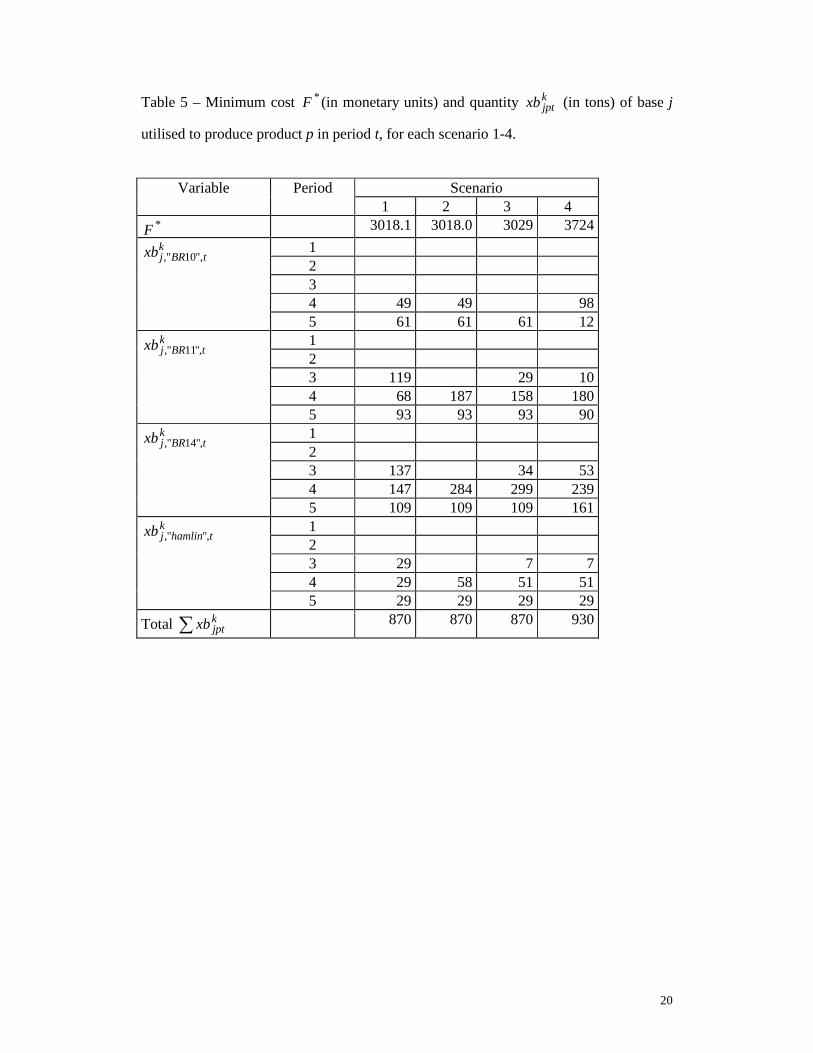
The minimum cost solution of model (1)-(11) yields *F = 3018.1 monetary units

(m.u.) as shown in table 5. Although all demands occur in period 5 (a total of 870 tons),

the products are produced in periods 3, 4 and 5 (table 5) because of the blending

capacity of only 292 tons per period. Observe that, as far as possible, this solution

avoids the blending and transportation of bases and products before the period of

demand (for example, all products are transported only in period 5 as presented in table

6).

Scenario 2

In scenario 2 we simply increased the blending capacity of period 4 from 292 to

870 tons, that is, equal to the demands of all products. The value of the minimum cost

solution of model (1)-(11) becomes *F = 3018.0 m.u. (table 5), which is lower than the

one of scenario 1 ( *F = 3018.1 m.u.) due to the need of anticipating the mix of bases

only in period 4, instead of periods 3 and 4 as in scenario 1 (table 5).

Scenario 3

In scenario 3 we reduced the capacity of the tank farms of the plant from 2790 to

800 tons. This way this capacity becomes a limitation in the third and fourth periods

11

(table 7) and it is necessary to blend and transport products to the external tank farms

(tables 5 and 6, respectively). The minimum cost solution with *F = 3029 m.u.

anticipates part of the blending of period 4 to period 3 (table 5), and part of the

transportation in bulk of period 5 to periods 3 and 4 (table 6). This changing yields an

additional cost of 11 m.u. with respect to scenario 2 (i.e., from 3018 to 3029 m.u.) due

to additional warehousing expenses outside the plant (table 7), and the financing cost of

anticipating the blending and transportation of products (tables 5 and 6). Note that as we

integrate the blending decisions in a distribution model, we allow the anticipation of the

production of products, followed by their immediate transportation to the external

warehouse.

Scenario 4

In scenario 4 we reduced the capacity of the external tank farms from 1650 to

200 tons in order to analyse the system performance when the production volume

exceeds the total (pant and external) tank farm capacity. As discussed in scenario 3, the

warehousing capacity of the plant tank farm becomes a limitation in the third and fourth

periods (table 7) and it is necessary to blend and transport products to the external tank

farms (tables 5 and 6, respectively). Moreover, the total capacities of the plant and

external tank farms are reached in the fourth period (table 7). This way, the model

determines the drumming of the production excess (160 tons as shown in table 6) at an

additional expense of 695 m.u. with respect to scenario 3 (i.e., from 3029 to 3724 m.u.

according to table 5).

Other scenarios

Other scenarios were investigated changing different parameters, such as the

percentage of base hamlin added to the final products, the cold storage (drums) capacity

of the plant, the initial inventories of products, etc. All solutions produced by model (1)-

(11) were consistent and reflected the expected behaviour of the system.

Evaluation of the goal programming model

In order to analyse the performance of model (2)-(14), we arbitrarily chose

scenario 4. Initially we solved model (2)-(14) considering only goal 1 (zero cost) in the

objective function (12), which, as expected, yielded the same minimum cost solution of

12

model (1)-(11) with value 3724*1 ==+ Fs m.u. (according to table 5). Then we solved

model (2)-(14) considering only goal 2 (mean ratio) in (12) and adding the constraint *

1 Fs =+ to the model (in accordance with the discussion of section 3), which results in

the minimum mean ratio deviation ( )∑∑∑ =+ −+

t k p

kpt

kpt ss 5.4022 . This deviation is much

smaller than the one of 224.0 obtained in the minimum cost solution of model (1)-(11),

showing that model (2)-(14), under the same value of goal 1, presents substantial

benefits from the point of view of goal 2. Table 8 compares the product quantities (in

tons) and ratios of periods 3-5 obtained by the two models (1)-(11) and (2)-(14).

5. Concluding remarks

In this study we propose a model based on linear and goal programming to

support medium to short term decisions in the process of blending bases for the

production of FCOJ, and the transportation and storage of the products. The model

utilises well-known concepts from the literature of blending problems and multistage,

multiproduct and multiperiod production planning problems. We mention the

importance of integrating blending decisions in a distribution model, since this allows

the anticipation of FCOJ production followed by its immediate transportation and

storage in external warehouses (as illustrated in scenario 3 of section 4). Despite being

based on a particular case study, we believe that the model is sufficiently generic or can

be easily extended for application to other orange juice companies.

An interesting perspective for future research is the application of the model for

the duration of one season (e.g., 51 weeks) in order to compare the solutions obtained by

the model with the ones adopted by the company. Another interesting research is to

integrate the present blending and distribution model to a harvest planning model, which

would result in a powerful tool for the analysis of tactical and operational decisions

from the orange fields until the vessel shipments of final products.

References

[1] Bazaraa, M.S., Jarvis, J.J. and Sherali, H.D. "Linear programming and network

flows". John Wiley & Sons, New York (1990).

13

[2] Brooke, A., Kendrick, D., Meeraus, A. and Rosenthal, R.E. "GAMS: A user’s

guide", Release 2.25". The Scientific Press (1992).

[3] FAO. "Food and agriculture organization of the United Nations: oranges

production". Source: http://apps.fao.org/lim 500/nph-

wrap.pl?Production.Crops.Primary&Domain=SUA&servlet=1 (printed in

01/02/2000).

[4] FAO. "Food and agriculture organization of the United Nations: orange juice

concentrated exports". Source: http://apps.fao.org/lim 500/nph-

wrap.pl?Trade.CropslivestockProduct&Domain=SUA&servlet=1 (printed in

02/02/2000).

[5] Hax, A.C. and Candea, D. "Production and inventory management". Prentice-Hall,

New Jersey (1984).

[6] Johnson, L.A. and Montgomery, D.C. "Operations research in production planning,

scheduling, and inventory control". John Wiley & Sons, New York (1974).

[7] Munhoz, J.R. "Um modelo baseado em programação linear e programação de metas

para análise de um sistema de produção e distribuição de suco concentrado

congelado de laranja". Dissertation, Universidade Federal de São Carlos, Brazil

(2000).

[8] Nahmias, S. "Production and operations analysis", 3rd ed. McGraw-Hill (1997).

[9] Pinto, K.C.R. "Contribuição à análise de decisão sobre os sistemas de distribuição

física de suco de laranja brasileiro de exportação". PhD. Thesis, Universidade de

São Paulo, Brazil (1996).

[10] Shapiro, J.F. "Mathematical programming models and methods for production

planning and scheduling". In: Graves, S.C., Rinnooy Kan, A.H.G and Zipkin, P.H.

(eds). Logistics of production and inventory (Handbooks in operations research and

management science: v.4), Elsevier Science (1993) 371-439.

[11] Viegas, F.C.P., Steger, E., Antonio, A.P., Fox, K.I. and Gray, L.E. "Processamento

dos produtos cítricos com máquinas FMC". FMC of Brazil (1983).

[12] Williams, H.P. "Model building in mathematical programming", 3rd ed. John Wiley

& Sons, New York (1993).

[13] Winston, W.L. "Operations research: applications and algorithms", 3rd ed.

Wadsworth, Belmont (1994).

14

Figure 1 - Basic plan of the season

Sales plan

Distribution plan Blending plan Initial inventories

Extraction plan

Fruit plan

15

Figure 2 - Blending of bases for the production of FCOJ (in bulk or drums),

transportation of FCOJ (in bulk or drums) from the plant warehouses to external

warehouses, and inventories of bases and FCOJ in the plant and external warehouses.

Base (in bulk): plant

Product (in bulk): plant

Product (drums): plant

Product (in bulk): external

Product (drums): external

16

Table 1 – Terminology utilised in the orange juice industry

Box of oranges Unit of weight equal to 40.8 kilograms or 90 pounds Brix Percentage of soluble solids or sugars and acids, quantified in brix

degrees by means of a refractometer Acidity After the sugars, the acids are the second more numerous soluble

solids in the orange juice Ratio Ratio brix/acidity which provides the maturity level and the quality of

the orange juice Variety The orange varieties pera, natal and valencia are the more indicated for

industrialisation. The variety hamlin allows the factory to economically operate in the beginning of the season because of its precocity, however it produces a low quality juice.

17

Table 2: Variables

Notation Description kjptxb Quantity (in tons) of base j utilised to produce product p in period t. This

quantity leaves the plant tank farm as base j (in bulk) and enters into the plant warehouse in form k (in bulk or drums) as product p

klptxt Quantity (in tons) of product p transported from the plant warehouse in form

k (in bulk or drums) to the external warehouse in form l (in bulk or drums) in period t

jteb Quantity (in tons) of base j in the plant tank farm at the end of period t kptepf Quantity (in tons) of product p in the plant warehouse in form k at the end of

period t lptepe Quantity (in tons) of product p in the external warehouse in form l at the end

of period t F Total cost of blending, transportation, warehousing and financing along the

planning horizon

18

Table 3: Parameters

Notation Description tb Capacity (in tons) of blending in the plant in period t

kab Capacity (in tons) of the plant warehouse in form k (supposed constant along the periods)

lat Capacity (in tons) of the external warehouse in form l (supposed constant along the periods)

jratb Mean ratio of base j

pratp Minimum ratio of product p kjcb Unit cost (in monetary units/tons) of utilising base j to produce a product in

form k (supposed constant along the periods) klpct Unit cost (in monetary units/tons) of transporting product p from the plant

warehouse in form k to the external warehouse in form l (supposed constant along the periods). In the cases of transportation from the plant tank farm (in bulk) to the external cold storage (drums), or from the plant cold storage (drums) to the external tank farm (in bulk), this unit cost includes the unit cost of packaging or unpackaging the product.

jhb Unit cost (in monetary units/tons) of storing base j in the plant tank farm (supposed constant along the periods)

kphpf Unit cost (in monetary units/tons) of storing product p in the plant

warehouse in form k (supposed constant along the periods) lphpe Unit cost (in monetary units/tons) of storing product p in the external

warehouse in form l (supposed constant along the periods) jtpr Production (in tons) of base j in period t

lptd Demand (in tons) of product p in the external warehouse in form l in period

t tperc Percentage of base hamlin added to the final products in period t

ktxb Unit cost (in monetary units/tons) of anticipating the blending in the plant warehouse in form k in one period

lptxt Unit cost (in monetary units/tons) of anticipating the transportation of

product p to the external warehouse in form l in one period

19

Table 4: Deviation (surplus and slack) variables

Notation Description +1s Deviation variable indicating how much the total costs of blending,

transporting, warehousing and financing are above goal 1: "zero cost". +kpts2 Deviation variable indicating how much product p in the plant warehouse in

form k in period t is above the specification of "mean ratio" desired by goal 2 (in tons x ratio).

−kpts2 Deviation variable indicating how much product p in the plant warehouse in

form k in period t is below the specification of "mean ratio" desired by goal 2 (in tons x ratio).

20

Table 5 – Minimum cost *F (in monetary units) and quantity kjptxb (in tons) of base j

utilised to produce product p in period t, for each scenario 1-4.

Scenario Variable Period 1 2 3 4

*F 3018.1 3018.0 3029 3724 1 2 3 4 49 49 98

ktBRjxb ,"10,"

5 61 61 61 12 1 2 3 119 29 10 4 68 187 158 180

ktBRjxb ,"11",

5 93 93 93 90 1 2 3 137 34 53 4 147 284 299 239

ktBRjxb ,"14",

5 109 109 109 161 1 2 3 29 7 7 4 29 58 51 51

kthamlinjxb ,"",

5 29 29 29 29 Total ∑ k

jptxb 870 870 870 930

21

Table 6 – Quantity klptxt (in tons) of product p transported from the plant warehouse in

form k (in bulk or drums) to the external warehouse in form l (in bulk or drums) in

period t, for each scenario 1-4.

Scenario Variable Period 1 2 3 4

1 2 3 4

"","","11"

drumdrumtPAxt

5 100 100 100 100 1 2 3 4

"","","12"bulkbulktPAxt

5 330 330 330 330 1 2 3 70 70 4 290 130

"","","13"bulkbulktPAxt

5 440 440 80 140 1 2 3 4 160

"","","13"drumbulktPAxt

5 Total ∑ kl

ptxt 870 870 870 930

22

Table 7 – Product inventories (in tons) in the plant and external warehouses at the end

of each period for scenarios 1-4.

Scenario Variable Period 1 2 3 4

1 290 290 290 2902 580 580 580 5803 870 870 800 8004 1160 1160 800 800

∑ ∑+p j

jtbulk

pt ebepf "" (plant)

5 290 290 290 2301 2 3 70 704 360 200

∑p

bulkptepe "" (external)

5 1 2 3 4 160

∑p

drumptepe "" (external)

5 60

23

Table 8 – Product quantities (in tons) and ratios of periods 3-5 obtained by models (1)-

(11) and (2)-(14) for scenario 4

Results Model (1)-(11) Model (2)-(14)

Period 3 Period 4 Period 5 Period 3 Period 4 Period 5

Product p

Mean ratio

Qt. Ratio Qt. Ratio Qt. Ratio Qt. Ratio Qt. Ratio Qt. RatioPAR11 (drum)

11.5 100 11.2 100 11.9

PAR12 (bulk)

12.5 144 12.9 186 12.9 38 12.5 292 12.5

PAR13 (bulk)

13.5 70 13.9 264 13.1 106 13.9 70 13.5 370 13.5

PAR13 (drum)

13.5 60 13.1 60 13.5