GEOPHYSICS, VOL. 66, NO. 2 (MARCH-APRIL 2001); P. 613–626, 10 FIGS.

A constrained global inversion method using an overparameterizedscheme: Application to poststack seismic data

Xin-Quan Ma∗

ABSTRACT

A global optimization algorithm using simulated an-nealing has advantages over local optimization ap-proaches in that it can escape from being trapped in localminima and it does not require a good initial model andfunction derivatives to find a global minimum. It is there-fore more attractive and suitable for seismic waveforminversion. I adopt an improved version of a simulated an-nealing algorithm to invert simultaneously for acousticimpedance and layer interfaces from poststack seismicdata. The earth’s subsurface is overparameterized by aseries of microlayers with constant thickness in two-waytraveltime. The algorithm is constrained using the low-frequency impedance trend and has been made compu-tationally more efficient using this a priori information asan initial model. A search bound of each parameter, de-rived directly from the a priori information, reduces thenonuniqueness problem. Application of this techniqueto synthetic and field data examples helps one recoverthe true model parameters and reveals good continuityof estimated impedance across a seismic section. This ap-proach has the capability of revealing the high-resolutiondetail needed for reservoir characterization when a reli-able migrated image is available with good well ties.

INTRODUCTION

Seismic inversion is the calculation of the earth’s structureand physical parameters from some sets of observed seismicdata. The output of the seismic inversion can be P-wave andS-wave velocities, Poisson’s ratio, or acoustic impedance vol-ume. The fundamental interpretive benefit of any form ofseismic inversion is that interface information is converted tointerval information. Hence, the final presentation is represen-tative of the geology, which is the study of rocks rather thanrock boundaries. An impedance volume is more readily tied to

Published on Geophysics Online August 28, 2000. Manuscript received by the Editor November 12, 1998; revised manuscript received December13, 1999.∗Scott Pickford Group Ltd., Seismic Technology Division, 7th Floor, Leon House, 233 High Street, Croydon CR0 9XT, United Kingdom. E-mail:frankm@scopic.com.c© 2001 Society of Exploration Geophysicists. All rights reserved.

well logs, for example, and more directly related to reservoirproperties. It permits reservoir properties to be interpretedbetween wells on a layer-by-layer basis using calibrations atwell locations. Acoustic impedance sections and volumes area valuable asset for exploration, appraisal, and developmentsince impedance is often a direct hydrocarbon indicator. Thedata are also useful for mapping fluids within the reservoir andimproving volumetric estimation. Acoustic impedance model-ing is also accepted as a valuable analytic tool for reservoircharacterization and 4-D time-lapse seismic studies.

Historically, the most popular seismic inversion techniqueused to estimate acoustic impedance is recursive inversion. Itis based on the well-known reflection coefficient formula interms of the adjacent acoustic impedances. However, to makethe algorithm work effectively, the seismic data must be freefrom the effects of the source wavelet, noise, multiples, spher-ical spreading, and transmission losses and only represent aband-limited, zero-phase sonic-log reflection coefficient series.Recursive inversion can only operate over the available seismicbandwidth. The upper frequency limit imposes a seismic res-olution restriction on the estimated acoustic impedance. Thelower limit indicates that inversion cannot generate absolutevalues of acoustic impedance but only relative ones. Absolutevalues of interval velocity are often determined from NMO andare combined with inverted velocity for a final output. How-ever, NMO velocity is only used on frequencies of up to about3 Hz.

Many inversion approaches are now based on forwardingmodeling. Synthetic seismograms are generated from an initialsubsurface model and compared to the real seismic data; themodel is modified, and the synthetic data are updated and com-pared to the real data again. If after many iterations no furtherimprovement is achieved, the updated model is the inversionresult. A priori information is usually incorporated to improvethe uniqueness of the output. Inversion is usually treated asa linear problem, that is, measurements are assumed to beara linear relation to the parameters. However, many geophysi-cal problems are nonlinear. Such problems are usually solved

613

614 Ma

by a sequence of linear approximations. A starting model isgiven, the misfit is used to perturb the model to make themisfit smaller, the new misfit is then used to further perturbthe model, and so on. Iterations are stopped when the misfitis smaller than a prescribed convergence tolerance or whensuccessive iterations fail to make any improvements. Typicalexamples of this inversion approach are the generalized lin-ear inversion method (Cooke and Schneider, 1983) and theMarquardt-Levenberg method (Tarantola and Valette, 1982;Lines and Treitel, 1984). These conventional local optimiza-tion methods require the determination of function derivatives.They are prone to trapping in local minima, and their successdepends heavily on the choice of starting model. This is becausethey rely on exploiting the limited information derived froma comparatively small number of models and avoid extensiveexploration of the model space. Some local methods find theminimum by taking an increment along the steepest gradient toarrive at the next approximation, the step length often beingproportional to the magnitude of the gradient. Convergenceassumes that the objective function is continuous and that theinitial estimate is already on the upper slopes of the correctglobal minimum. Local methods find the nearest minimum ofthe objective function, which may not be the global minimumor the true model. If the starting model has a misfit that iswithin the valley of the global minimum, then linearized inver-sion will descend the walls of that valley to that minimum bymaking small perturbations to the starting model. However, ifyou start in the wrong valley, the iterative search diverges fromthe global minimum. The linearized inversion normally endsup with a final model that differs only slightly from the startingmodel.

Because of the highly band-limited nature of seismic data,the objective function normally contains many valleys. We wishto find the lowest valley by searching widely through the modelspace. This problem belongs to the category of global optimiza-tion. Global methods, usually using a Monte Carlo randomprocess, require no derivatives information and do not assumethat the objective function has a particular shape. Simulated an-nealing is one of the most widely used global methods, operat-ing analogously to thermodynamic systems. It is usually imple-mented by a drunkard’s walk through the model space, wheresteps begin in random fashion but are progressively biased to-ward the global minimum (Corana et al., 1987; Sen and Stoffa,1991; Goffe et al., 1994). Another class of global methods iscalled genetic algorithms. They try to evolve a trial populationof models in a way similar to biological evolution (Goldberg,1989; Stoffa and Sen, 1991). Global methods in general avoidthe limitations of local methods and are particularly attractivein model-driven seismic waveform inversion.

Inversion of poststack seismic data using simulated anneal-ing is described by Vestergaard and Mosegaard (1991). Theyuse an improved version of the simulated annealing algorithmby Nulton and Salamon (1998) in which statistical informationabout the system to be optimized is used to improve the per-formance of the algorithm. They restrict the simulated anneal-ing optimization to the two-way traveltime parameters to lo-cate interfaces and perform a simple, linear optimization (leastsquares) to reflection coefficients. The objective function is asingle-term L2-norm misfit between the modelled and observedseismic traces. A weak reflection coefficient constraint is alsoapplied to the algorithm using minimum and maximum reflec-

tion coefficients. The output from their optimization algorithmis reflection coefficients series; acoustic impedance traces mustbe obtained using a conventional recursive formula given a sur-face impedance value. While the use of a linear optimization toreflection coefficient parameters is computationally efficient,reflection coefficients, unlike acoustic impedance, are difficultto constrain because bounds for reflection coefficients as a func-tion of two-way traveltimes are difficult to derive from a prioribackground information. Furthermore, the success of convert-ing the finally optimized reflection coefficients into acousticimpedance traces critically depends on the starting impedancevalue.

In this paper I use an improved version of simulated anneal-ing by Corana et al. (1987) and Goffe et al. (1994) to invert theacoustic impedance for 1-D earth models (applications to 2-Dand 3-D models do not involve any fundamentally differenttheory). The global optimization applies not only to acousticimpedances but also to the two-way traveltimes (interfaces).The algorithm is constrained by including an additional termin the objective function prohibiting the final solution driftingaway from the a priori background low-frequency trend. Thecomputational efficiency is enhanced by starting the algorithmfrom an a priori impedance trend. Meanwhile, the nonunique-ness problem is reduced by restricting impedance perturba-tions within sensible bounds, which are derived directly fromthe background impedance trend. Since impedance valuesalong with interfaces are solved simultaneously by the globaloptimization, the output are the absolute acoustic impedancevalues within the optimum interfaces; the surface impedancevalue, normally used by other algorithms for the recursivecalculation of impedance from reflection coefficients, is notrequired.

To illustrate the robustness of the simulated annealing algo-rithm used in this paper, I examine the effects on the resolvedimpedance and interfaces of initial models and the selectedseeds for the random number generator, and I show why theglobal optimization algorithm does not depend on the initialmodel and particular paths the random process has followed. Ialso show how to deduce a critical initial temperature for sim-ulated annealing using statistical information during trial runs.The developed method is applied to a synthetic data example ofideally blocky layers and also to field data where well data areavailable for estimating the source wavelet and constructinginitial models.

SIMULATED ANNEALING

Simulated annealing is a global optimization technique thatmimics the physical process by which a crystal is grown byslow cooling of melt until the global minimum energy state isreached. It explores the objective function’s surface and tries tooptimize the function while moving both uphill and downhill.In standard annealing, a random point in the model space is se-lected and the energy f or misfit is calculated. The new modelis accepted unconditionally if the energy associated with thenew point f ′ is lower (� f = f ′ − f < 0). If the new point hasa higher misfit (� f > 0), then it is accepted with the proba-bility p = exp(−� f/T ), where T is a control parameter calledacceptance temperature. The generation–acceptance process isrepeated several times at a fixed temperature. Then the temper-ature is lowered following a cooling schedule, and the process

Constrained Global Inversion 615

is repeated. The algorithm is stopped when the error doesnot change after a sufficient number of trials (see Appendix).This acceptance criterion is known as the Metropolis rule(Metropolis et al., 1953). Since the probability of acceptinga step in an uphill direction is always greater than zero, thealgorithm can climb out of a local minimum. This is in contrastto the local search methods in which a new model is acceptedonly if � f < 0, i.e., it always searches in the downhill direction.Given a high starting temperature, simulated annealing firstbuilds a rough view of the objective function surface. Whenthe temperature is decreased, the algorithm progresses to re-duce to zero the probability of accepting a bad step as the globalminimum is reached (Figure 1).

FIG. 1. A flow diagram of an improved simulated annealingoptimization routine.

The modifications made by Corana et al. (1987) to the stan-dard simulated annealing methods include a model pertur-bation controlled by a step length (refer to the Appendix).This step length is determined from the statistical informationdrawn during a number of iterations and is adjusted automat-ically to sample the objective function widely and to focus at-tention on the most promising area in the model space. Theadjustment is made such that at least 50% of all moves ineach coordinate direction are accepted. If a greater percent-age of moves is accepted, the relevant element of a step-lengthvector is enlarged. This increases the number of rejectionsand decreases the percentage of acceptance. After many timesthrough the above adjustment loops, T is reduced (Figure 1). Alower temperature makes a given uphill move less likely, so thenumber of acceptances decreases and the step lengths decline.The algorithm is stopped when the difference between severalrecorded optima is less than a given convergence tolerance (seethe Appendix).

The step-length adjustment has many advantages over otherversions of simulated annealing methods in that it providesvaluable information about the function’s flatness or rough-ness and increases the accuracy of parameter solutions. If anelement of a step-length vector remains large, the functionis flat in that parameter. Further extensions of the above al-gorithms are introduced by Goffe et al. (1994). One modi-fication checks if the global optimum is indeed achieved byusing different seeds for the random number generator. An-other extension lets us determine a critical initial tempera-ture for the algorithm by examining the step-length changeduring a trial run. This minimizes the execution time of thealgorithm.

A proper selection of a starting temperature T0 is crucialto implementing the simulated annealing method because theglobal method is computationally intensive. If the initial tem-perature is too low, the step length will be too small and thearea containing the global optimum may be missed. If too high,then the step length will be too large and an excessively largearea will be searched, wasting computing resources.

FORWARD MODELING

To apply optimization algorithms to the inversion problem,one must find a model to generate synthetic seismograms sothat a misfit between the observed and synthetic can be de-termined. In laterally homogeneous acoustic media, seismicpropagation can be approximately modelled by the convolu-tion theory:

S(t) =∫ ∞

−∞R(τ )W (t − τ ) dτ, (1)

where S(t) is a seismic trace as a function of two-way trav-eltime, W (t) is the seismic wavelet, and R(t) is the reflec-tion coefficients series. This mathematical model establishes arelationship between the poststack seismic data and the un-known model parameters such as velocity, density, acousticimpedance, and locations of interfaces. However, a properanalysis of the seismic data must include the effects of geomet-rical divergence, anelastic absorption, dispersion of wavelet,transmission losses across the boundaries of the layered me-dia, and multiple reflections. For this paper in which the con-volutional model is applied in a relatively small time window,

616 Ma

these complications are ignored and I assume the convolutionalmodel is adequate.

The seismic source wavelet is usually unknown but can beestimated using various techniques—for example, the partialcoherence method of White (1980). In this paper, I use a zero-phase Ricker wavelet of 35 Hz for testing the inversion of syn-thetic earth models but a wavelet estimated by the partial co-herence method using both seismic and well data for testingthe inversion of the real data. The synthetic seismic data arecalculated in the frequency domain using forward and inversefast Fourier transforms (FFTs).

OBJECTIVE FUNCTION

Optimization procedures require a misfit criterion or objec-tive function to evaluate the quality of each trial model. Theoptimum model is determined when the objective function is inthe global minimum or maximum, dependent on which type ofobjective function is used. The choice of the measure of misfitis crucial to the success of the process. Two types of objectivefunctions are widely used in seismic waveform inversion. One isthe correlation coefficient type, representing the resemblanceof the observed and synthetic seismic data, which leads to amaximization problem (Sen and Stoffa, 1991). The other oneis the least-squares type, representing the difference betweenthe observed and synthetic data (the L2-norm), which defines aminimization problem (Lines and Treitel, 1984). While the ad-vantage of the correlation-based objective function is that theinversion results are less sensitive to noise, the least-squarestype has proven to show much better results (Huang, 1996).An objective function may contain multiple terms, allowingdifferent types of constraints to be built into the model. This iscrucially important in improving the completeness and unique-ness of inverted results. In seismic waveform inversion, thelow-frequency impedance and lateral continuity constraints arecommonly used to reduce the nonuniqueness problem and im-prove the lateral coherence of the solution. In this paper, I usethe L1-norm error function, the least absolute deviation be-tween the observed and modelled seismic trace. The L1-normerror function can avoid overweighing large residuals as theL2-norm does. I also build in an a priori information constraintas a second term in the objective function, which forces the so-lution to be close to the low-frequency impedance trend. Theobjective function is expressed as

� f = W1

n∑i=1

∣∣Siobs − Si

mod

∣∣ + W2

m∑i=1

∣∣Pipri − Pi

mod

∣∣, (2)

where Siobs is the observed seismic data, Si

mod is the syntheticseismic data, Pi

pri is an a priori low-frequency impedance trend,Pi

mod is the modelled impedance, n is the number of samples inthe seismic trace, m is the number of microlayers in the initialmodel, and W1 and W2 are weights applied to the two terms,respectively.

LAYER PARAMETERIZATION

The earth’s impedance is a continuous function in depth. Itis often advantageous to make a discrete approximation to thiscontinuous function. If lithology boundaries are known, an ob-vious discrete approximation is to sample the earth medium as

separate layers; the layer thickness is assumed to be known,and we solve for the impedance in each layer (we often referto this impedance representation as exact parameterization).When lithology boundaries are unknown, the earth model canbe sampled as a number of microlayers with constant thickness,and both layer interfaces and impedance need to be solved. Ifthe total number of microlayers is larger than that of the trueearth medium, this representation is defined as overparame-terization. Another category is the full-scale parameterizationby which the earth model is sampled at the same interval ofequal two-way traveltime as in seismic data. This is the extremecase of overparameterization, requiring a very large number ofimpedance unknowns—but no layer boundaries—to solve.

While the exact parameterized scheme appears to be supe-rior in terms of its simplicity, in practice it is difficult to im-plement because the layer interfaces are not generally knownexactly; we are often required to invert uninterpreted seismicdata and to extract more detailed information, including thelayer boundaries. Even if the data have been interpreted, somehuman error is certain to be introduced because of the band-width limitation of seismic data and structures complicated bythinning beds, faulting, and intrusive features. Since the verti-cal resolution of the inverted impedance profile is expected tobe greater than the seismic data, the use of exact parameteri-zation based on preinterpreted horizons may limit the verti-cal resolution of the inverted earth impedance profile. Thefull-scale parameterization also appears to be appealing be-cause one needs to concentrate on impedance only. However,the main drawback of this scheme is its high computationalcost from the increasing number parameters. Furthermore, thisscheme introduces instability into final solutions resulting fromthe nonuniqueness problem (Sen and Stoffa, 1991).

I concentrate on the overparameterized scheme, which ismore practical for real applications. The earth model is de-scribed by a series of interconnected microlayers; each micro-layer is described by its thickness or two-way traveltime andimpedance. In this scheme, both impedance and interfaces areconsidered as unknown parameters and are solved simultane-ously by the global optimization procedure.

SYNTHETIC DATA EXAMPLE

An earth model is assumed to consist of ten layers overly-ing a half-space. Each layer is assigned a constant impedancevalue and layer thickness. The impedance ranges from 2 to8 (g/cm3 × km/s), while the thickness in two-way traveltimeranges from 20 to 60 ms (Figure 2a). The observed seismicdata in this experiment are calculated using the reflection co-efficients of the true earth model convolved with a zero-phaseRicker wavelet of 35 Hz (Figure 2b). We have also obtainedthe low-frequency impedance curve by band-pass filtering(0–5 Hz) the true impedance data. The objective function con-sists of the least absolute deviation between the observed andsynthetic seismic data and the least absolute deviation betweenthe low-frequency and modelled impedance. The former is themisfit function; the latter is an a priori impedance constraint.Layer parameterization is performed assuming the earth ismade up of 21 horizontal microlayers including the underly-ing half-space. Since the number of microlayers is greater thanthat of the model, this is an overparameterized scheme. The un-known parameters to be optimized consist of 21 impedances

Constrained Global Inversion 617

and 20 interfaces. This is to say that we have an objective func-tion with 41 variables (parameters) and need to resolve them,given the observed seismic data and a wavelet, so that the resul-tant 41 parameters produce a global minimum of the objectivefunction.

Global optimization is achieved using the modified simu-lated annealing routine described above. To apply the algo-rithm, one needs to supply the objective function, lower andupper parameter boundaries, initial model parameters (or astarting model), initial annealing temperature, and a conver-gence tolerance. The initial model parameters consist of 20interfaces at microlayer boundaries and 21 impedance valuestaken from the low-frequency impedance trend. The simu-lated annealing algorithm begins by calculating the objec-tive function using the initial model parameters and then ac-cepting or rejecting this move using the Metropolis criteria.Within a given temperature many iterations are allowed tobe performed, and the step length is adjusted according tothe statistics drawn from those iterations. The temperature islowered until the convergence tolerance is satisfied. The out-puts are the optimized impedance values and locations of layerinterfaces.

While the global method does not depend heavily on thestarting model, it does requires physically sensible bounds torestrict the parameter searching space as a result of the multi-modal nature of the objective function. A good selection of pa-rameter boundaries reduces the nonuniqueness problem andminimizes the computing time. In this experiment, we allowthe impedance parameters to lie within ±2.5 (g/cm3 × km/s)around the low-frequency trend and the two-way traveltimeswithin±12 ms around microlayer boundaries. The convergencetolerance ε should be chosen with reference to the objective

FIG. 2. (a) A 1-D earth model consisting of 10 layers overlying a half-space. Each layer is described by constant acoustic impedanceand thickness in two-way traveltime. (b) A Ricker wavelet with a principal frequency of 35 Hz.

function values, for example, 0.1% of the objective functionvalue at the first iteration in simulated annealing.

The inverted impedance and interfaces are shown in Fig-ure 3a. The inversion results match well with the true earthmodel, with relative errors less than 3%. The synthetic seismictrace calculated using the inverted impedance profile has alsobeen plotted along with the observed and error traces (Fig-ure 3b). They indicate that nearly all energy in the observedtrace has been inverted, resulting in an almost zero-error trace.To illustrate the evolution of the simulated annealing proce-dure, I show four intermediate results from annealing. The ini-tial annealing temperature is taken as 0.1 and is subsequentlyreduced according to the rule described in the Appendix.The inverted impedance profiles are plotted against the trueimpedance depth function after 1000, 5000, 10 000, and 15 000iterations (Figure 4a). Although the match at the 1000th it-eration is very poor, the impedance function follows the gen-eral trend of the low-frequency impedance profile because ofthe initial model and parameter search bounds imposed. Af-ter 5000 iterations, the impedance values within layers 2, 3,and 9 get close to the true impedance. After 10 000 iterations,not only impedance but also interfaces of all 11 layers arenear to the optimum solution. The last 5000 iterations tunethe results further, and by the end of 15 000 iterations an op-timum solution is found. To reveal how the misfit is reducedthrough the evolution of annealing, I plot the synthetic seis-mic trace against the observed seismic data after 1000, 5000,10 000, and 15 000 iterations (Figure 4b). The quality of matchincreases as the number of iterations increases. By the endof 15 000 iterations, almost all energy in the observed seismictrace has been recovered, resulting in an optimum impedancesolution.

618 Ma

Many factors determine the total number of iterations re-quired for the algorithm to reach the final equilibrium. Amongthem are the initial temperature T0 and convergence toler-ance ε. There are other parameters: Ns , Nt , Nε , and rT , crit-ically control the efficiency of the algorithm. The meanings ofthese parameters are fully explained in the Appendix. WhileCorana et al. (1987) use Ns = 20, Nt = max(100, 5n), Nε = 4,and rT = 0.85 in their function tests, I found that in this seis-mic inversion exercise the parameters can be smaller. My testsshow that I can choose Ns = 10, Nt = 3, Nε = 3, and rT = 0.5and get equally satisfactory results. This modification substan-tially reduces the total number of iterations without sacrificingaccuracy. This means that to invert the impedance profile inFigure 3a using the newly modified parameters requires 18 700iterations, in contrast to 32 800 iterations if Corana’s parametervalues are used. I also found that setting the initial step lengthsequal to 25% of the initial model parameters will speed up theconvergence.

Simulated annealing, unlike local optimization methods suchas gradient descent and downhill simplex, does not rely on theinitial parameters. As a matter of fact, most conventional sim-ulated annealing codes use randomly distributed parametersto start with, and the optimization continues until the conver-gence tolerance is satisfied. To illustrate the dependency ofsolutions upon the initial model, I rerun the optimization rou-tine for the earth model shown in Figure 2a but use differentinitial parameters. The results using an initial model that de-viates from the general trend of true impedance is shown inFigure 5a. Although the initial model is close to the lower

FIG. 3. (a) Comparison between the true earth impedance profile (solid line) and that inverted by an overparameterized scheme(dotted line). An initial model contains 20 microlayers with impedance values defined by the low-frequency trend. Initial temperaturefor simulated annealing is T0 = 0.1. (b) The original, inverted, and error seismic traces.

parameter boundary, the impedance and interface are still re-solved with high accuracy. If the initial model is set to be close tothe upper parameter boundary, the results are hardly affected(Figure 5b). Therefore, it is advantageous to use the globaloptimization method for seismic waveform inversion in caseswhere well control is sparse or where the correlation betweenseismic events and nearby wells is made difficult by fault zones,thinning beds, or the presence of strong noise. However, theindependence of initial models is achieved partially by using arelatively high initial temperature, which allows the algorithmto search a wide area (more uphill moves accepted) but as aconsequence increases the computational burden. In practice,if near-optimal solutions or a priori information are available,it is always beneficial to use this information in the startingmodels. This is because starting from a near-optimum modeldoes not require a high initial temperature and saves a lot ofcomputing time.

As mentioned earlier, in running the simulated annealingprogram, one needs an initial temperature T0, a key parametercontrolling the efficiency of the simulated annealing operatorand the resolution of modelled parameters. While a large T0

permits a wide space to be searched, it produces more accep-tances and fewer rejections. This may impose a large computa-tional burden and make the method less efficient. On the otherhand, a small T0 may make it difficult for the current solution toescape from the local minimum, which risks that the solutionyou have found is not in the global optimum. While trial anderror is always suggested to obtain the optimal T0, the improvedsimulated annealing routine presented in this paper allows us to

Constrained Global Inversion 619

a)

b)

FIG. 4. (a) Four intermediate stages of simulated annealing. Solid lines are the true impedance profiles, while dashed lines arethe inverted impedance profiles. Iterations 1000, 5000, 10 000, and 15 000 correspond to the annealing temperatures at 1.00 × 10−1,1.25 × 10−2, 1.56 × 10−3, and 9.76 × 10−5, respectively. (b) The match between the synthetic seismic trace and the observed seismictrace at the four stages.

620 Ma

examine the step length of each parameter and hence guidesus to choose an appropriate starting temperature through afew trial runs. I have rerun the above model using a very highstarting temperature, T0 = 1000, and monitored the step-lengthvariation for parameters 2, 10, and 20 with falling temperature.

FIG. 5. (a) Same as Figure 3a except that the starting impedance parameters are chosen to be close to the lower parameter bound.(b) Starting parameters are close to the upper parameter bound.

FIG. 6. (a) Relationship between step length and annealing temperature for three parameters. This is used to determine the criticaltemperature for the simulated annealing procedure. (b) Relationship between the objective function and number of global minimumupdates as a function of seeds for the random number generator. This shows the convergence of the solution through differentpaths.

The step length here corresponds to the impedance parame-ter for a specific layer. The relationship between step lengthand temperature is shown in Figure 6a. One can see that thestep length changes very little at the earlier stage of anneal-ing (T < 1.0) and starts to fall only when the temperature gets

Constrained Global Inversion 621

around 0.1. This temperature (T = 0.1 in this case) is oftentermed as a critical temperature from which more effectivesearches really begin. Prior to the critical temperature, manyfunction evaluations are carried out and too many acceptancesare made, resulting in a considerable waste of computing re-sources. In this example, an appropriate starting temperatureshould be chosen as T0 = 0.1. However, the critical tempera-ture determined may also be dependent on which parameteris being monitored. One should always choose the maximumcritical temperature among all the parameters monitored as astarting temperature for the annealing procedure.

Apart from the influences of an initial temperature T0 andstarting models, the simulated annealing procedure is also af-fected by the use of different seeds for the random number gen-erator. This is because a different seed enables the algorithm tofollow a completely different path. In theory, no matter whatseed is used, the convergence to the same global minimumshould take place. In practice a slight difference in solutionsshould be expected because of the different paths the algorithmhas followed. To illustrate this point, I have run the optimiza-tion routine four times using four different seeds (Figure 3a).At each run, the number of updates to the global minimumand their associated objective function values are plotted inFigure 6b. In the earlier updates, the objective function valuesare almost the same; later, they converge to the global min-imum through different paths. This is because in the earlierstage, for a fixed temperature, the algorithm searches parame-ters near the initial model, which gives similar function values.As the temperature decreases, the objective function is reducedtoward the global minimum. The exact path the algorithm fol-lows depends on the nature of the objective function and thetype of the random generator. However, one can rerun the al-gorithm with the same initial temperature and different seeds.If the same optimum is found within an accepted tolerance,there is a high degree of confidence in the global optimumfound.

FIELD DATA EXAMPLE

The seismic data were from a North Sea 3-D survey andhad been processed using conventional data processing meth-ods including spherical divergence correction, deconvolution,multiple suppression and prestack migration. Four wells hadP-wave velocity logs available. Following are inversion resultsfor a single seismic trace near the well and for an in-line seismiccross-section.

A wavelet estimate is required before optimization proce-dures can be implemented. We assume the seismic trace isequivalent to the earth’s reflectivity convolved with a station-ary wavelet plus an amount of noise. The well data give us theearth’s reflectivity at the well locations. Comparing the seismicdata at these locations, to a synthetic trace will yield an esti-mate of the wavelet. The wavelet is the matching filter betweenthe log and seismic segments and is computed using the auto-,cross-, and power spectra of both segments (White, 1980). Thismethod also quantifies the quality of match between the syn-thetic seismogram and the data and hence indicates the validityof the convolutional model. The wavelet estimated at one ofthe wells is shown in Figure 7.

As described in the synthetic data example, we also needthe low-frequency impedance trend to constrain our inversion.

This low-frequency trend was generated using all the well dataand the seismic horizon data. A velocity function of the formV = V0 + k Z was determined for each of the interpreted unitsbetween the horizons, where V0 is the velocity at the horizontalsurface datum, V is the velocity at a depth Z below the datumplane, and k is a constant whose value is generally between0.3/s and 1.3/s . This function was then interpolated for all CDPbins; for each of these, a velocity trace in time was generated.The velocity volume was then converted to impedance usingGardner’s equation.

The results from the inversion of a single seismic trace neara well are shown in Figure 8. Only a 400-ms data window isused. The low-frequency impedance is used as a constraint inthe objective function and to determine the lower and upperbounds of impedance within which the impedance parametersare allowed to perturb. Using an overparameterized scheme asdescribed in the synthetic data example, the earth is assumed toconsist of 23 microlayers including the underlying half-space,which yields 22 interfaces. These 45 parameters are optimizedusing the simulated annealing procedure with an initial tem-perature T0 = 0.1; results are shown in Figure 8a. The majorhorizons at 120, 225, 250, and 285 ms have been well predicted.The impedance match between the inverted seismic sectionand log is reasonably good except at 360–390 ms, where largerimpedance is predicted. The mismatch may be attributable toeither inaccuracy in log data or an unremoved multiple event inseismic data. The original, synthetic, and error seismic tracesare shown in Figure 8b. Some residuals still exist within theerror trace.

I also applied this single trace inversion technique to someof the in-line sections in this field—for example, section595 (Figure 9a). Optimization parameters such as the initialannealing temperature, interface perturbation window, and

FIG. 7. A source wavelet estimated using the partial coherencematching of synthetic seismograms with real seismic data.

622 Ma

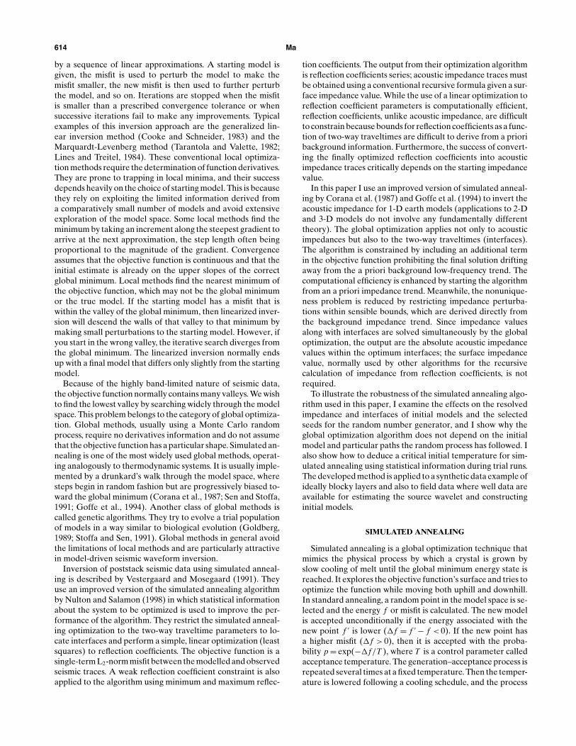
FIG. 8. (a) Comparison between impedance log (dotted line) and inversion by an overparameterized scheme (solid line). Impedanceis in g/cm3 × km/s. An initial model contains 22 microlayers with impedance values defined by the low-frequency trend. Initialtemperature for simulated annealing is 0.1, and the total number of iterations is around 19 000. (b) The original, synthetic, and errorseismic traces. The starting time of the data window is from 0, which corresponds to 2000 ms in the real data set.

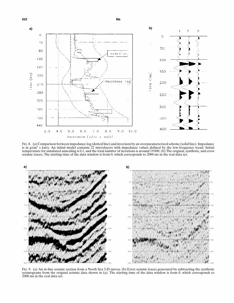
FIG. 9. (a) An in-line seismic section from a North Sea 3-D survey. (b) Error seismic traces generated by subtracting the syntheticseismograms from the original seismic data shown in (a). The starting time of the data window is from 0, which corresponds to2000 ms in the real data set.

Constrained Global Inversion 623

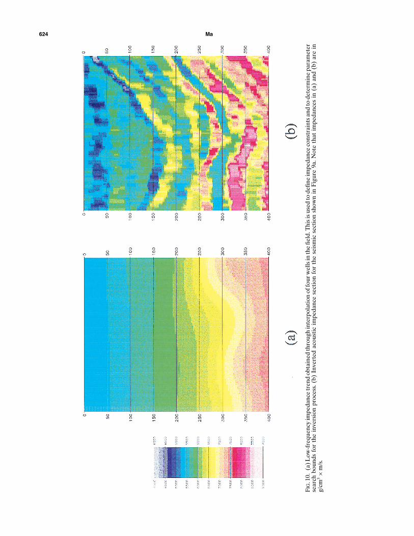
convergence tolerance are determined from the above exercisefor the single trace near the well location (Figure 8) in whichthe true impedance log is available to control the quality ofinversion. The low-frequency impedance trend (Figure 10a) isused as the initial model and defines constraints for the ob-jective function. The absolute impedance inverted and errorseismic traces are shown in Figures 10b and 9b, respectively.The inverted impedance corresponds well to seismic events,and lateral variations of seismic impedance values within layersare evident. Trace-to-trace continuity of inverted impedance isvery high, demonstrating the stability of the method. Consis-tent layer boundaries have also been derived.

In the above real-data example, I chose 23 microlayers overa 400-ms data window as an initial model. The result shows thatthe match between the inverted and log impedance is reason-ably good. But is this overparameterized? How do we choosethe number of microlayers if there is little direct knowledgeabout this parameter from real data?

The first criterion for choosing the total number of micro-layers is that the layers should be thin enough for the syntheticdata to mimic the real data. An underparameterized scheme, inwhich the microlayers modelled are thicker than the layeringof the real medium, is more likely to produce a large misfit be-tween the synthetic and observed seismic data (Sen and Stoffa,1991). On the other hand, while very thin microlayers are morelikely to achieve a low misfit or a better match, the impedancesolution may not necessarily be unique (the nonuniquenessproblem is discussed in detail at the end of this paper). Fur-thermore, a consequence of using very thin microlayers is that alarge number of parameters are generated, which makes the al-gorithm less efficient. This leads to the second criterion, i.e., themicrolayers should not be so thin that the computational timebecomes impractical and the solutions unstable. The instabilityproblem caused by using very thin layers or too many layerswithin a short time distance is discussed in detail by Sen andStoffa (1991). In their test examples, 21 microlayers represent afour-layer model. Their results show that although the correla-tion values obtained are very high (low misfit), the constructedmodels differ considerably from the true model. The inversionalgorithm picked many contrasting velocity and density val-ues in the homogeneous part of the model and generated apoor match of impedances at the real layer boundaries. Theyconclude that when the model is overparameterized, many dif-ferent models explain the observed seismic data.

To determine the exact number of microlayers as an ini-tial model satisfying the above two criteria is difficult in prac-tice. However, a guideline can be adopted from analyzing thefrequency spectrum of seismic data. The higher frequency ofcomponent the seismic data carries, the higher resolution andhence more details about the earth structure it reveals. There-fore, we should use thinner layers for high-frequency data thanfor low-frequency data. When impedance logs are available,seismic traces near well locations should be inverted first usingdifferent microlayer thicknesses. This helps us determine anoptimum microlayer thickness through the quality control ofan inverted impedance trace against an impedance log.

NONUNIQUENESS

Seismic inversion is nonunique, that is, a number of differentmodels can lead to the same set of observations. This is true

partly because measurements are incomplete and also becausethey involve uncertainties. In model-driven seismic inversion,the quality of a solution is determined by comparing the ob-served seismic trace to a synthetic trace generated from thesolution. If these two are the same, then the solution is exactbut not necessarily unique. For the overparameterized schemepresented in this paper, the earth is parameterized by a se-ries of impedances and interfaces. Perturbation of either pa-rameters will change the waveform of synthetic data. Withoutany constraints, this could lead to the situation that there aremany combinations of impedance and interfaces, all satisfyingthe perfect match between the observed and synthetic data.The acoustic impedance solution from seismic inversion is ex-tremely nonunique in the frequency ranges outside the band-width of the source wavelet. This phenomenon can be viewedfrom the low and high ends of frequency bandwidths. Considerthat the main frequencies recorded range from approximately10 to 60 Hz. Very low-frequency information about the acous-tic impedance, say, <8 Hz, is not directly derivable from band-limited seismic data. Since reflection coefficients are negligi-ble derived from a smooth, low-frequency impedance trace,its contribution to the synthetic seismic amplitudes after theconvolution with a band-limited wavelet is negligible, too. In amodel-driven inversion scheme without constraints, many so-lutions with different low-frequency trends all equally satisfythe observation. The inversion process also rejects any frequen-cies higher than the wavelet bandwidth, say, >60 Hz. Considera sufficiently thin bed embedded in a homogeneous half-space.Such an impedance structure produces two reflection coeffi-cients of opposite polarity and equal amplitude. The convolu-tion of these reflection coefficients with a band-limited waveletcontributes little to the synthetic seismic amplitudes. Any num-ber of thin beds can be added to the acoustic impedance profilewithout significantly affecting the fit to the data. The very high-frequency content is therefore impossible to recover throughinversion.

Despite the nonuniqueness problem encountered in seis-mic inversion, constraints usually limit the physical propertiessuch that the set of possible solutions exists only within nar-row bounds. For my inversion scheme, these constraints areachieved by using a priori impedance information, that definesthe parameter search boundaries and also guides the solution,moving toward the physically meaningful trend. Interfaces arealso constrained by allowing them to perturb within a narrowtime window. The low-frequency impedance data can be ob-tained using both well logs and seismic processing velocity data.From the optimization perspective, while global methods suchas simulated annealing and genetic algorithms are less depen-dent on the initial model, they do require sensible parameterbounds. Incorporating a priori information into the inversionscheme can therefore speed up the convergence and stabilizethe solution considerably.

CONCLUSIONS

Global optimization methods, based on a stochastic searchmechanism, do not require derivatives information and a goodinitial model to find the global optimum. They can escape frombeing trapped in local minima by moving both downhill anduphill. This is in contrast to conventional local methods, whichuse the gradient information and need a good initial guess to

624 Ma

FIG

.10.

(a)L

ow-f

requ

ency

impe

danc

etr

end

obta

ined

thro

ugh

inte

rpol

atio

nof

four

wel

lsin

the

field

.Thi

sisu

sed

tode

fine

impe

danc

eco

nstr

aint

sand

tode

term

ine

para

met

erse

arch

boun

dsfo

rth

ein

vers

ion

proc

ess.

(b)

Inve

rted

acou

stic

impe

danc

ese

ctio

nfo

rth

ese

ism

icse

ctio

nsh

own

inFi

gure

9a.N

ote

that

impe

danc

esin

(a)

and

(b)

are

ing/

cm3×

m/s

.

Constrained Global Inversion 625

guide their search. Global methods such as simulated anneal-ing and genetic algorithms are therefore more attractive andsuitable for model-driven seismic waveform inversion.

The improved simulated annealing algorithm described inthis paper has many advantages over the standard simulatedannealing algorithm in terms of its robustness and computa-tional efficiency. The step-length adjustment adopted duringthe cooling schedule allows us to monitor and study the func-tion behavior and helps us find the critical initial temperature.This algorithm can find optimum solutions with high precisionand is particularly robust in solving seismic inversion problems.The algorithm has been made computationally efficient by tun-ing annealing parameters to fit the seismic inversion scheme.

I have applied the simulated annealing algorithm to theinversion of a 1-D earth model using an overparameterizedscheme in which the earth’s subsurface is parameterized by a se-ries of microlayers with constant impedance within each layer.The algorithm has been accelerated by using the low-frequencyimpedance trend as the starting point, and the nonuniquenessproblem has been reduced by assigning a boundary to each pa-rameter. Since the impedance bounds are derived directly fromthe low-frequency trend, the output is the absolute impedancevalues within optimized microlayer boundaries. Application ofthis scheme to synthetic and field data examples reveal a goodmatch between inverted and true impedance for a single traceand impedance profiles with good continuity and stability. Thistechnique has the capability of extracting maximum resolu-tion of the acoustic impedance over typical reservoir intervals,making it a suitable tool for reservoir characterization and 4-Dtime-lapse seismic studies.

The inversion approach described in this paper can be usedwhenever forward modeling can be implemented, for example,prestack seismic inversion via amplitude variation with offset(AVO).

ACKNOWLEDGMENTS

The author thanks Paul Haskey and Adrian Pelham of ScottPickford Group Ltd. for stimulating discussions and readingthe manuscript.

REFERENCES

Cooke, D. A., and Schneider, W. A., 1983, Generalized linear inversionof reflection seismic data: Geophysics, 48, 665–676.

Corana, A., Marchesi, M., Martini, C., and Ridella, S., 1987, Minimiz-ing multimodal functions of continuous variables with the simulatedannealing algorithm: ACM Trans. of Math. Soft., 13, 262–280.

Goffe, W. L., Ferrier, G. D., and Rogers, J., 1994, Global optimisationof statistical functions with simulated annealing: J. Economet., 60,65–100.

Goldberg, D. E., 1989, Genetic algorithms in search, optimisation andmachine learning: Addison-Wesley Publ. Co.

Huang, X., 1996, Seismic inversion using heuristic combinatorial algo-rithm: A hybrid scheme: 66th Ann. Internat. Mtg., Soc. Expl. Geo-phys., Expanded Abstracts, 1963–1966.

Lines, L. R., and Treitel, S., 1984, A review of least-squares inversionand its application to geophysical problems: Geophys. Prosp., 32,159–186.

Metropolis, N., Rosenbluth, A., Rosenbluth, M., Teller, A., and Teller,E., 1953, Equation of state calculations by fast computing machines:J. Chem. Phys., 21, 1087–1092.

Nulton, J. D., and Salamon, P., 1988, Statistical mechanics of combina-torial optimisation: Physics Rev., A37, 1351–1356.

Sen, M. K., and Stoffa, P. L., 1991, Nonlinear one-dimensional seis-mic waveform inversion using simulated annealing: Geophysics, 56,1624–1638.

Stoffa, P. L., and Sen, M. K., 1991, Nonlinear multiparameter optimiza-tion using genetic algorithms: Inversion of plane-wave seismograms:Geophysics, 56, 1974–1810.

Tarantola, A., and Valette, B., 1982, Generalised nonlinear inverseproblems solved using the least squares criterion: Rev. Geophys.Space Phys., 20, 219–232.

Vestergaard, P. D., and Mosegaard, K., 1991, Inversion of post-stackseismic data using simulated annealing: Geophys. Prosp., 39, 613–624.

White, R. E., 1980, Partial coherence matching of synthetic seismo-grams with seismic traces: Geophys. Prosp., 28, 333–358.

APPENDIX

AN IMPROVED SIMULATED ANNEALING ALGORITHM

Let X be a vector and (x1, x2, . . . , xn) its components.Let f (x) be the objective function to minimize, and leta1 < x1 < b1, . . . , an < xn < bn be its n variables, each rangingin a finite, continuous interval. Simulated annealing proceedsinteractively. Starting from a given point X0, it generates a suc-cession of points: X0, X1, . . . , Xi , . . . tending to the global min-imum of the objective function. Let us assume that the cur-rently accepted solution is X and the function value is f . Newcandidate points are generated around the current point xi , inturn applying random moves along each coordinate direction(Corana et al., 1987):

x ′ = xi + rvi ,

where r is a uniformly distributed random number from [−1, 1]and vi is element i of a step-length vector V = (v1, v2, . . . , vn).If the point falls outside the definition boundary, a new pointis randomly generated until a point belonging to the definitiondomain is found:

x ′ = ai + r(bi − ai ).

The function value f ′ is then computed. If f ′ is less than f, X′

is accepted unconditionally and the algorithm moves down-hill. If this is the smallest function value, X′ is recorded as thebest current value of the optimum. If f ′ is greater or equal

to f , the Metropolis criterion decides on acceptance with theprobability

p = e−( f ′− f )/T

where T is temperature and p is compared to p′, a uniformlydistributed random number from [0, 1]. If p < p′, the new point(X′) is accepted and the algorithm moves uphill; otherwise, X′

is rejected. Both a low temperature and a large difference inthe function values decrease the probability of an uphill move.

After Ns steps through all elements of X, the step-length vec-tor V is adjusted to better follow the function behavior. Theaim of these variations in step length is to maintain the aver-age percentage of accepted moves at about one-half of the totalnumber of moves (Corana et al., 1987). For each direction i thenew step-vector component v′

i is

v′i = vi

(1 + ci

ni/Ns − 0.60.4

)if ni > 0.6 Ns,

v′i = vi

1 + ci0.4 − ni/Ns

0.4

if ni < 0.4 Ns,

v′i = vi otherwise.

626 Ma

The value vi is the current step length, ci is a parameter con-trolling the step variation along each ith direction, and ni is thenumber of accepted moves along the ith direction as a resultof total Ns trials. The ratio ni/Ns is therefore restricted to theinterval [0, 1].

If a greater percentage of moves is accepted for xi , then therelevant element of V is enlarged. For a given temperature thisincreases the number of rejections and decreases the percent-age of acceptances. From an optimization view, a high numberof accepted moves with respect to rejected ones means thefunction is explored with too small steps. On the other hand,a high number of rejected moves means that new trial pointsare generated too far from the current point. A 1 : 1 ratio be-tween accepted and rejected moves ensures that the algorithmis following the function behavior well.

After Nt · Ns cycles of moves along every direction with Nt

step-length adjustments (refer to Figure 1), T is reduced. Thenew temperature is given by

T ′ = rT · T,

where rT is the temperature reduction factor set between 0 and1. A lower temperature makes a given uphill move less likely,so the number of rejections increases and the step lengths de-cline. In addition, the first point tried at the new temperatureis the current optimum. The smaller step length and starting at

the current optimum focuses attention on the most promisingarea.

The process ends by comparing the last Nε values of thesmallest function values from the end of each temperature re-duction with the most recent one and the current optimumfunction value. If all these differences are less than a prescribedtolerance, the process terminates. If these conditions are notsatisfied, the algorithm starts again through all steps describedabove.

Apart from the initial temperature and convergence toler-ance, other factors such as Ns , Nt , ci , Nε , and rT also control theefficiency of the simulated annealing. Some test optimizationsof simple functions made by Corana et al. (1987) suggest thefollowing values should be used:

Ns = 20,

Nt = max(100, 5n),

ci = 2, i = 1, 2, . . . , n,

Nε = 4,

rT = 0.85.

However, much smaller values for rT and Nt were chosen byGoffe et al. (1994) in the optimization tests, and their resultswere equally satisfactory.