Fine-Grained Analysis of Optimization and Generalization forOverparameterized Two-Layer Neural Networks

Sanjeev Arora * 1 2 Simon S. Du * 3 Wei Hu * 1 Zhiyuan Li * 1 Ruosong Wang * 3

AbstractRecent works have cast some light on the mys-tery of why deep nets fit any data and generalizedespite being very overparametrized. This paperanalyzes training and generalization for a simple2-layer ReLU net with random initialization, andprovides the following improvements over recentworks:

(i) Using a tighter characterization of trainingspeed than recent papers, an explanation forwhy training a neural net with random la-bels leads to slower training, as originallyobserved in [Zhang et al. ICLR’17].

(ii) Generalization bound independent of net-work size, using a data-dependent complex-ity measure. Our measure distinguishesclearly between random labels and true la-bels on MNIST and CIFAR, as shown byexperiments. Moreover, recent papers re-quire sample complexity to increase (slowly)with the size, while our sample complexity iscompletely independent of the network size.

(iii) Learnability of a broad class of smooth func-tions by 2-layer ReLU nets trained via gradi-ent descent.

The key idea is to track dynamics of training andgeneralization via properties of a related kernel.

1. IntroductionThe well-known work of Zhang et al. (2017) highlightedintriguing experimental phenomena about deep net train-ing – specifically, optimization and generalization – andasked whether theory could explain them. They showed

*Alphabetical order 1Princeton University, Princeton, NJ, USA2Institute for Advanced Study, Princeton, NJ, USA 3CarnegieMellon University, Pittsburgh, PA, USA. Correspondence to: WeiHu <huwei@cs.princeton.edu>.

Proceedings of the 36 th International Conference on MachineLearning, Long Beach, California, PMLR 97, 2019. Copyright2019 by the author(s).

that sufficiently powerful nets (with vastly more parametersthan number of training samples) can attain zero trainingerror, regardless of whether the data is properly labeled orrandomly labeled. Obviously, training with randomly la-beled data cannot generalize, whereas training with properlylabeled data generalizes. See Figure 2 replicating some ofthese results.

Recent papers have begun to provide explanations, showingthat gradient descent can allow an overparametrized multi-layer net to attain arbitrarily low training error on fairlygeneric datasets (Du et al., 2018a;c; Li & Liang, 2018; Allen-Zhu et al., 2018b; Zou et al., 2018), provided the amountof overparametrization is a high polynomial of the relevantparameters (i.e. vastly more than the overparametrization in(Zhang et al., 2017)). Under further assumptions it can alsobe shown that the trained net generalizes (Allen-Zhu et al.,2018a). But some issues were not addressed in these papers,and the goal of the current paper is to address them.

First, the experiments in (Zhang et al., 2017) show thatthough the nets attain zero training error on even randomdata, the convergence rate is much slower. See Figure 1.

Question 1. Why do true labels give faster convergencerate than random labels for gradient descent?

The above papers do not answer this question, since theirproof of convergence does not distinguish between goodand random labels.

The next issue is about generalization: clearly, some prop-erty of properly labeled data controls generalization, butwhat? Classical measures used in generalization theorysuch as VC-dimension and Rademacher complexity aremuch too pessimistic. A line of research proposed norm-based (e.g. (Bartlett et al., 2017a)) and compression-basedbounds (Arora et al., 2018). But the sample complexityupper bounds obtained are still far too weak. Furthermorethey rely on some property of the trained net that is re-vealed/computed at the end of training. There is no propertyof data alone that determine upfront whether the trained netwill generalize. A recent paper (Allen-Zhu et al., 2018a)assumed that there exists an underlying (unknown) neuralnetwork that achieves low error on the data distribution, andthe amount of data available is quite a bit more than the min-

Fine-Grained Analysis of Optimization and Generalization for Overparameterized Two-Layer Neural Networks

imum number of samples needed to learn this underlyingneural net. Under this condition, the overparametrized net(which has way more parameters) can learn in a way thatgeneralizes. However, it is hard to verify from data whetherthis assumption is satisfied, even after the larger net hasfinished training.1 Thus the assumption is in some senseunverifiable.Question 2. Is there an easily verifiable complexity measurethat can differentiate true labels and random labels?

Without explicit regularization, to attack this problem, onemust resort to algorithm-dependent generalization analysis.One such line of work established that first-order methodscan automatically find minimum-norm/maximum-marginsolutions that fit the data in the settings of logistic regres-sion, deep linear networks, and symmetric matrix factor-ization (Soudry et al., 2018; Gunasekar et al., 2018a;b;Ji & Telgarsky, 2018; Li et al., 2018b). However, howto extend these results to non-linear neural networks re-mains unclear (Wei et al., 2018). Another line of algorithm-dependent analysis of generalization (Hardt et al., 2015;Mou et al., 2017; Chen et al., 2018) used stability of specificoptimization algorithms that satisfy certain generic proper-ties like convexity, smoothness, etc. However, as the numberof epochs becomes large, these generalization bounds arevacuous.

Our results. We give a new analysis that provides answersto Questions 1 and 2 for overparameterized two-layer neuralnetworks with ReLU activation trained by gradient descent(GD), when the number of neurons in the hidden layer issufficiently large. In this setting, Du et al. (2018c) haveproved that GD with random initialization can achieve zerotraining error for any non-degenerate data. We give a morerefined analysis of the trajectory of GD which enables us toprovide answers to Questions 1 and 2. In particular:

• In Section 4, using the trajectory of the network pre-dictions on the training data during optimization, weaccurately estimate the magnitude of training loss ineach iteration. Our key finding is that the number ofiterations needed to achieve a target accuracy dependson the projections of data labels on the eigenvectorsof a certain Gram matrix to be defined in Equation (3).On MNIST and CIFAR datasets, we find that such pro-jections are significantly different for true labels andrandom labels, and as a result we are able to answerQuestion 1.

• In Section 5, we give a generalization bound for thesolution found by GD, based on accurate estimates ofhow much the network parameters can move duringoptimization (in suitable norms). Our generalization

1In Section 2, we discuss the related works in more details.

bound depends on a data-dependent complexity mea-sure (c.f. Equation (10)), and notably, is completely in-dependent of the number of hidden units in the network.Again, we test this complexity measure on MNIST andCIFAR, and find that the complexity measures for trueand random labels are significantly different, whichthus answers Question 2.Notice that because zero training error is achieved bythe solution found by GD, a generalization bound is anupper bound on the error on the data distribution (testerror). We also remark that our generalization bound isvalid for any data labels – it does not require the exis-tence of a small ground-truth network as in (Allen-Zhuet al., 2018a). Moreover, our bound can be efficientlycomputed for any data labels.

• In Section 6, we further study what kind of functionscan be provably learned by two-layer ReLU networkstrained by GD. Combining the optimization and gener-alization results, we uncover a broad class of learnablefunctions, including linear functions, two-layer neuralnetworks with polynomial activation �(z) = z

2l or co-sine activation, etc. Our requirement on the smoothnessof learnable functions is weaker than that in (Allen-Zhuet al., 2018a).

Finally, we note that the intriguing generalization phenom-ena in deep learning were observed in kernel methods aswell (Belkin et al., 2018). The analysis in the current pa-per is also related to a kernel from the ReLU activation(c.f. Equation (3)).

2. Related WorkIn this section we survey previous works on optimizationand generalization aspects of neural networks.

Optimization. Many papers tried to characterize geomet-ric landscapes of objective functions (Safran & Shamir,2017; Zhou & Liang, 2017; Freeman & Bruna, 2016; Hardt& Ma, 2016; Nguyen & Hein, 2017; Kawaguchi, 2016;Venturi et al., 2018; Soudry & Carmon, 2016; Du & Lee,2018; Soltanolkotabi et al., 2018; Haeffele & Vidal, 2015).The hope is to leverage recent advance in first-order algo-rithms (Ge et al., 2015; Lee et al., 2016; Jin et al., 2017)which showed that if the landscape satisfies (1) all localminima are global and (2) all saddle points are strict (i.e.,there exists a negative curvature), then first-order methodscan escape all saddle points and find a global minimum.Unfortunately, these desired properties do not hold even forsimple non-linear shallow neural networks (Yun et al., 2018)or 3-layer linear neural networks (Kawaguchi, 2016).

Another approach is to directly analyze trajectory of the op-timization method and to show convergence to global mini-

Fine-Grained Analysis of Optimization and Generalization for Overparameterized Two-Layer Neural Networks

mum. A series of papers made strong assumptions on inputdistribution as well as realizability of labels, and showedglobal convergence of (stochastic) gradient descent for someshallow neural networks (Tian, 2017; Soltanolkotabi, 2017;Brutzkus & Globerson, 2017; Du et al., 2017a;b; Li &Yuan, 2017). Some local convergence results have also beenproved (Zhong et al., 2017; Zhang et al., 2018). However,these assumptions are not satisfied in practice.

For two-layer neural networks, a line of papers used meanfield analysis to establish that for infinitely wide neuralnetworks, the empirical distribution of the neural networkparameters can be described as a Wasserstein gradientflow (Mei et al., 2018; Chizat & Bach, 2018a; Sirignano &Spiliopoulos, 2018; Rotskoff & Vanden-Eijnden, 2018; Weiet al., 2018). However, it is unclear whether this frameworkcan explain the behavior of first-order methods on finite-sizeneural networks.

Recent breakthroughs were made in understanding opti-mization of overparameterized neural networks throughthe trajectory-based approach. They proved global poly-nomial time convergence of (stochastic) gradient descent onnon-linear neural networks for minimizing empirical risk.Their proof techniques can be roughly classified into twocategories. Li & Liang (2018); Allen-Zhu et al. (2018b);Zou et al. (2018) analyzed the trajectory of parameters andshowed that on the trajectory, the objective function satisfiescertain gradient dominance property. On the other hand,(Du et al., 2018a;c) analyzed the trajectory of network pre-dictions on training samples and showed that it enjoys astrongly-convex-like property.

Generalization. It is well known that the VC-dimensionof neural networks is at least linear in the number of pa-rameters (Bartlett et al., 2017b), and therefore classical VCtheory cannot explain the generalization ability of mod-ern neural networks with more parameters than trainingsamples. Researchers have proposed norm-based general-ization bounds (Bartlett & Mendelson, 2002; Bartlett et al.,2017a; Neyshabur et al., 2015; 2017; 2019; Konstantinoset al., 2017; Golowich et al., 2017; Li et al., 2018a) andcompression-based bounds (Arora et al., 2018). Dziugaite& Roy (2017); Zhou et al. (2019) used the PAC-Bayes ap-proach to compute non-vacuous generalization bounds forMNIST and ImageNet, respectively. All these bounds areposterior in nature – they depend on certain properties ofthe trained neural networks. Therefore, one has to finishtraining a neural network to know whether it can general-ize. Comparing with these results, our generalization boundonly depends on training data and can be calculated withoutactually training the neural network.

Another line of work assumed the existence of a true model,and showed that the (regularized) empirical risk minimizer

has good generalization with sample complexity that de-pends on the true model (Du et al., 2018b; Ma et al., 2018;Imaizumi & Fukumizu, 2018). These papers ignored thedifficulty of optimization, while we are able to prove gener-alization of the solution found by gradient descent. Further-more, our generic generalization bound does not assume theexistence of any true model.

Our paper is closely related to (Allen-Zhu et al., 2018a)which showed that two-layer overparametrized neural net-works trained by randomly initialized stochastic gradientdescent can learn a class of infinite-order smooth functions.In contrast, our generalization bound depends on a data-dependent complexity measure that can be computed forany dataset, without assuming any ground-truth model. Fur-thermore, as a consequence of our generic bound, we alsoshow that two-layer neural networks can learn a class ofinfinite-order smooth functions, with a less strict require-ment for smoothness. Allen-Zhu et al. (2018a) also studiedthe generalization performance of three-layer neural nets.

Lastly, our work is related to kernel methods, especiallyrecent discoveries of the connection between deep learn-ing and kernels (Jacot et al., 2018; Chizat & Bach, 2018b;Daniely et al., 2016; Daniely, 2017). Our analysis utilizedseveral properties of a related kernel from the ReLU activa-tion (c.f. Equation (3)).

3. Preliminaries and Overview of ResultsNotation. We use bold-faced letters for vectors and matri-ces. For a matrix A, let Aij be its (i, j)-th entry. We usek·k2 to denote the Euclidean norm of a vector or the spectralnorm of a matrix, and use k·kF to denote the Frobenius normof a matrix. Denote by �min(A) the minimum eigenvalue ofa symmetric matrix A. Let vec (A) be the vectorization of amatrix A in column-first order. Let I be the identity matrixand [n] = {1, 2, . . . , n}. Denote by N (µ,⌃) the Gaussiandistribution with mean µ and covariance ⌃. Denote by � (·)the ReLU function � (z) = max{z, 0}. Denote by I{E}the indicator function for an event E.

3.1. Setting: Two-Layer Neural Network Trained byRandomly Initialized Gradient Descent

We consider a two-layer ReLU activated neural networkwith m neurons in the hidden layer:

fW,a(x) =1pm

mX

r=1

ar��w

>r x�,

where x 2 Rd is the input, w1, . . . ,wm 2 Rd are weightvectors in the first layer, a1, . . . , am 2 R are weightsin the second layer. For convenience we denote W =(w1, . . . ,wm) 2 Rd⇥m and a = (a1, . . . , am)> 2 Rm.

Fine-Grained Analysis of Optimization and Generalization for Overparameterized Two-Layer Neural Networks

We are given n input-label samples S = {(xi, yi)}ni=1

drawn i.i.d. from an underlying data distribution D overRd ⇥ R. We denote X = (x1, . . . ,xn) 2 Rd⇥n andy = (y1, . . . , yn)> 2 Rn. For simplicity, we assume thatfor (x, y) sampled from D, we have kxk2 = 1 and |y| 1.

We train the neural network by randomly initialized gradientdescent (GD) on the quadratic loss over data S. In particular,we first initialize the parameters randomly:

wr(0) ⇠ N (0,2I), ar ⇠ unif ({�1, 1}) , 8r 2 [m],

(1)where 0 < 1 controls the magnitude of initialization,and all randomnesses are independent. We then fix thesecond layer a and optimize the first layer W through GDon the following objective function:

�(W) =1

2

nX

i=1

(yi � fW,a(xi))2. (2)

The GD update rule can be written as:2

wr(k + 1)�wr(k) = �⌘@�(W(k))

@wr

= � ⌘arpm

nX

i=1

(fW(k),a(xi)� yi)I�wr(k)

>xi � 0

xi,

where ⌘ > 0 is the learning rate.

3.2. The Gram Matrix from ReLU Kernel

Given {xi}ni=1, we define the following Gram matrix H1 2Rn⇥n as follows:

H1ij = Ew⇠N (0,I)

⇥x>i xjI

�w

>xi � 0,w>

xj � 0 ⇤

=x>i xj

�⇡ � arccos(x>

i xj)�

2⇡, 8i, j 2 [n].

(3)This matrix can be viewed as a Gram matrix from a kernelassociated with the ReLU function, and has been studiedin (Xie et al., 2017; Tsuchida et al., 2017; Du et al., 2018c).

In our setting of training a two-layer ReLU network, Duet al. (2018c) showed that if H1 is positive definite, GDconverges to 0 training loss if m is sufficiently large:Theorem 3.1 ((Du et al., 2018c)3). Assume �0 =

�min(H1) > 0. For � 2 (0, 1), if m = ⌦⇣

n6

�40

2�3

⌘and

⌘ = O��0n2

�, then with probability at least 1 � � over the

random initialization (1), we have:

• �(W(0)) = O(n/�);2Since ReLU is not differentiable at 0, we just define “gradient”

using this formula, and this is indeed what is used in practice.3Du et al. (2018c) only considered the case = 1, but it is

straightforward to generalize their result to general at the priceof an extra 1/2 factor in m.

• �(W(k + 1)) ⇣1� ⌘�0

2

⌘�(W(k)), 8k � 0.

Our results on optimization and generalization also cruciallydepend on this matrix H

1.

3.3. Overview of Our Results

Now we give an informal description of our main results.It assumes that the initialization magnitude is sufficientlysmall and the network width m is sufficiently large (to bequantified later).

The following theorem gives a precise characterization ofhow the objective decreases to 0. It says that this processis essentially determined by a power method for matrixI� ⌘H

1 applied on the label vector y.

Theorem 3.2 (Informal version of Theorem 4.1). With highprobability we have:

�(W(k)) ⇡ 1

2

��(I� ⌘H1)ky

��22, 8k � 0.

As a consequence, we are able to distinguish the conver-gence rates for different labels y, which can be determinedby the projections of y on the eigenvectors of H1. Thisallows us to obtain an answer to Question 1. See Section 4for details.

Our main result for generalization is the following:

Theorem 3.3 (Informal version of Theorem 5.1). For any1-Lipschitz loss function, the generalization error of thetwo-layer ReLU network found by GD is at most

r2y>(H1)�1y

n. (4)

Notice that our generalization bound (4) can be computedfrom data {(xi, yi)}ni=1, and is completely independent ofthe network width m. We observe that this bound can clearlydistinguish true labels and random labels, thus providing ananswer to Question 2. See Section 5 for details.

Finally, using Theorem 3.3, we prove that we can use ourtwo-layer ReLU network trained by GD to learn a broadclass of functions, including linear functions, two-layer neu-ral networks with polynomial activation �(z) = z

2l or co-sine activation, etc. See Section 6 for details.

3.4. Additional Notation

We introduce some additional notation that will be used.

Define ui = fW,a(xi), i.e., the network’s prediction on thei-th input. We also use u = (u1, . . . , un)

> 2 Rn to denoteall n predictions. Then we have �(W) = 1

2 ky � uk22 and

Fine-Grained Analysis of Optimization and Generalization for Overparameterized Two-Layer Neural Networks

the gradient of � can be written as:

@�(W)

@wr=

1pmar

nX

i=1

(ui � yi)Ir,ixi, 8r 2 [m], (5)

where Ir,i = I�w

>r xi � 0

.

We define two matrices Z and H which will play a key rolein our analysis of the GD trajectory:

Z =1pm

0

B@I1,1a1x1 · · · I1,na1xn

.... . .

...Im,1amx1 · · · Im,namxn

1

CA 2 Rmd⇥n,

and H = Z>Z. Note that

Hij =x>i xj

m

mX

r=1

Ir,iIr,j , 8i, j 2 [n].

With this notation we have a more compact form of thegradient (5):

vec (r�(W)) = Z(u� y).

Then the GD update rule is:

vec (W(k + 1)) = vec (W(k))� ⌘Z(k)(u(k)� y), (6)

for k = 0, 1, . . .. Throughout the paper, we use k as the itera-tion number, and also use k to index all variables that dependon W(k). For example, we have ui(k) = fW(k),a(xi),Ir,i(k) = I

�wr(k)>xi � 0

, etc.

4. Analysis of Convergence RateAlthough Theorem 3.1 already predicts linear convergenceof GD to 0 loss, it only provides an upper bound on theloss and does not distinguish different types of labels. Inparticular, it cannot answer Question 1. In this section wegive a fine-grained analysis of the convergence rate.

Recall the loss function �(W) = 12 ky � uk22. Thus, it

is equivalent to study how fast the sequence {u(k)}1k=0converges to y. Key to our analysis is the observation thatwhen the size of initialization is small and the networkwidth m is large, the sequence {u(k)}1k=0 stays close toanother sequence {u(k)}1k=0 which has a linear updaterule:

u(0) = 0,

u(k + 1) = u(k)� ⌘H1 (u(k)� y) ,

(7)

where H1 is the Gram matrix defined in (3).

Write the eigen-decomposition H1 =

Pni=1 �iviv

>i ,

where v1, . . . ,vn 2 Rn are orthonormal eigenvectors ofH

1 and �1, . . . ,�n are corresponding eigenvalues. Ourmain theorem in this section is the following:

Theorem 4.1. Suppose �0 = �min(H1) > 0, =

O

⇣✏�pn

⌘, m = ⌦

⇣n7

�40

2�4✏2

⌘and ⌘ = O

��0n2

�. Then with

probability at least 1� � over the random initialization, forall k = 0, 1, 2, . . . we have:

ky � u(k)k2 =

vuutnX

i=1

(1� ⌘�i)2k�v>i y�2 ± ✏. (8)

The proof of Theorem 4.1 is given in Appendix C.

In fact, the dominating termqPn

i=1(1� ⌘�i)2k�v>i y�2

is exactly equal to ky � u(k)k2, which we prove in Sec-tion 4.1.

In light of (8), it suffices to understand how fastPn

i=1(1�⌘�i)2k

�v>i y�2 converges to 0 as k grows. Define

⇠i(k) = (1 � ⌘�i)2k(v>i y)

2, and notice that each se-quence {⇠i(k)}1k=0 is a geometric sequence which startsat ⇠i(0) = (v>

i y)2 and decreases at ratio (1 � ⌘�i)2. In

other words, we can think of decomposing the label vec-tor y into its projections onto all eigenvectors vi of H1:kyk22 =

Pni=1(v

>i y)

2 =Pn

i=1 ⇠i(0), and the i-th portionshrinks exponentially at ratio (1� ⌘�i)2. The larger �i is,the faster {⇠i(k)}1k=0 decreases to 0, so in order to havefaster convergence we would like the projections of y ontotop eigenvectors to be larger. Therefore we obtain the fol-lowing intuitive rule to compare the convergence rates ontwo sets of labels in a qualitative manner (for fixed kyk2):

• For a set of labels y, if they align with the top eigen-vectors, i.e., (v>

i y)2 is large for large �i, then gradient

descent converges quickly.

• For a set of labels y, if the projections on eigenvectors{�v>i y�2}ni=1 are uniform, or labels align with eigen-

vectors with respect to small eigenvalues, then gradientdescent converges with a slow rate.

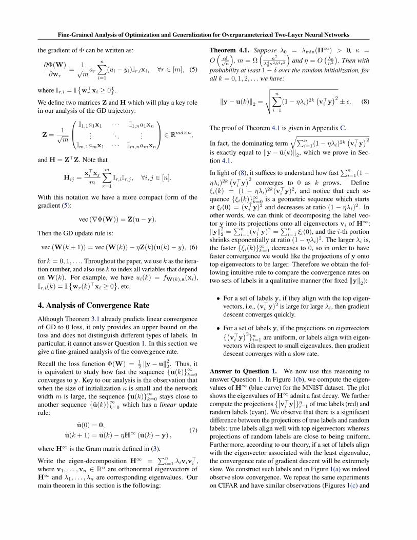
Answer to Question 1. We now use this reasoning toanswer Question 1. In Figure 1(b), we compute the eigen-values of H1 (blue curve) for the MNIST dataset. The plotshows the eigenvalues of H1 admit a fast decay. We furthercompute the projections {

��v>i y��}ni=1 of true labels (red) and

random labels (cyan). We observe that there is a significantdifference between the projections of true labels and randomlabels: true labels align well with top eigenvectors whereasprojections of random labels are close to being uniform.Furthermore, according to our theory, if a set of labels alignwith the eigenvector associated with the least eigenvalue,the convergence rate of gradient descent will be extremelyslow. We construct such labels and in Figure 1(a) we indeedobserve slow convergence. We repeat the same experimentson CIFAR and have similar observations (Figures 1(c) and

Fine-Grained Analysis of Optimization and Generalization for Overparameterized Two-Layer Neural Networks

(a) Convergence Rate, MNIST. (b) Eigenval & Projections, MNIST. (c) Convergence Rate, CIFAR. (d) Eigenval & Projections, CIFAR.

Figure 1: In Figures 1(a) and 1(c), we compare convergence rates of gradient descent between using true labels, randomlabels and the worst case labels (normalized eigenvector of H1 corresponding to �min(H1). In Figures 1(b) and 1(d), weplot the eigenvalues of H1 as well as projections of true, random, and worst case labels on different eigenvectors of H1.The experiments use gradient descent on data from two classes of MNIST or CIFAR. The plots clearly demonstrate that truelabels have much better alignment with top eigenvectors, thus enjoying faster convergence.

1(d)). These empirical findings support our theory on theconvergence rate of gradient descent. See Appendix A forimplementation details.

4.1. Proof Sketch of Theorem 4.1

Now we prove ky � u(k)k22 =Pn

i=1(1� ⌘�i)2k�v>i y�2.

The entire proof of Theorem 4.1 is given in Appendix C,which relies on the fact that the dynamics of {u(k)}1k=0 isessentially a perturbed version of (7).

From (7) we have u(k+ 1)� y = (I� ⌘H1) (u(k)� y),

which implies u(k) � y = (I � ⌘H1)k (u(0)� y) =

�(I � ⌘H1)ky. Note that (I � ⌘H

1)k has eigen-decomposition (I� ⌘H

1)k =Pn

i=1(1� ⌘�i)kviv>i and

that y can be decomposed as y =Pn

i=1(v>i y)vi. Then

we have u(k) � y = �Pn

i=1(1 � ⌘�i)k(v>i y)vi, which

implies ku(k)� yk22 =Pn

i=1(1� ⌘�i)2k(v>i y)

2.

5. Analysis of GeneralizationIn this section, we study the generalization ability of thetwo-layer neural network fW(k),a trained by GD.

First, in order for optimization to succeed, i.e., zero trainingloss is achieved, we need a non-degeneracy assumption onthe data distribution, defined below:Definition 5.1. A distribution D over Rd ⇥ R is (�0, �, n)-non-degenerate, if for n i.i.d. samples {(xi, yi)}ni=1 from D,with probability at least 1� � we have �min(H1) � �0 >

0.Remark 5.1. Note that as long as no two xi and xj areparallel to each other, we have �min(H1) > 0. (See (Duet al., 2018c)). For most real-world distributions, any twotraining inputs are not parallel.

Our main theorem is the following:Theorem 5.1. Fix a failure probability � 2 (0, 1). Sup-pose our data S = {(xi, yi)}ni=1 are i.i.d. samples from

a (�0, �/3, n)-non-degenerate distribution D, and =O��0�n

�,m �

�2poly�n,�

�10 , �

�1�. Consider any loss

function ` : R ⇥ R ! [0, 1] that is 1-Lipschitz in the firstargument such that `(y, y) = 0. Then with probability atleast 1� � over the random initialization and the trainingsamples, the two-layer neural network fW(k),a trained by

GD for k � ⌦⇣

1⌘�0

log n�

⌘iterations has population loss

LD(fW(k),a) = E(x,y)⇠D⇥`(fW(k),a(x), y)

⇤bounded as:

LD(fW(k),a)

s2y> (H1)�1

y

n+O

0

@

slog n

�0�

n

1

A .

(9)

The proof of Theorem 5.1 is given in Appendix D and wesketch the proof in Section 5.1.

Note that in Theorem 5.1 there are three sources of possi-ble failures: (i) failure of satisfying �min(H1) � �0, (ii)failure of random initialization, and (iii) failure in the datasampling procedure (c.f. Theorem B.1). We ensure that allthese failure probabilities are at most �/3 so that the finalfailure probability is at most �.

As a corollary of Theorem 5.1, for binary classificationproblems (i.e., labels are ±1), we can show that (9) alsobounds the population classification error of the learnedclassifier. See Appendix D for the proof.

Corollary 5.2. Under the same assumptions as in The-orem 5.1 and additionally assuming that y 2 {±1}for (x, y) ⇠ D, with probability at least 1 � �,the population classification error L

01D (fW(k),a) =

Pr(x,y)⇠D⇥sign

�fW(k),a(x)

�6= y⇤

is bounded as:

L01D (fW(k),a)

s2y> (H1)�1

y

n+O

0

@

slog n

�0�

n

1

A .

Fine-Grained Analysis of Optimization and Generalization for Overparameterized Two-Layer Neural Networks

(a) MNIST Data. (b) CIFAR Data.

Figure 2: Generalization error (`1 loss and classificationerror) v.s. our complexity measure when different portionsof random labels are used. We apply GD on data from twoclasses of MNIST or CIFAR until convergence. Our com-plexity measure almost matches the trend of generalizationerror as the portion of random labels increases. Note that `1loss is always an upper bound on the classification error.

Now we discuss our generalization bound. The dominatingterm in (9) is: s

2y> (H1)�1y

n. (10)

This can be viewed as a complexity measure of data thatone can use to predict the test accuracy of the learned neuralnetwork. Our result has the following advantages: (i) ourcomplexity measure (10) can be directly computed givendata {(xi, yi)}ni=1, without the need of training a neuralnetwork or assuming a ground-truth model; (ii) our boundis completely independent of the network width m.

Evaluating our completixy measure (10). To illustratethat the complexity measure in (10) effectively determinestest error, in Figure 2 we compare this complexity measureversus the test error with true labels and random labels (andmixture of true and random labels). Random and true labelshave significantly different complexity measures, and as theportion of random labels increases, our complexity measurealso increases. See Appendix A for implementation details.

5.1. Proof Sketch of Theorem 5.1

The main ingredients in the proof of Theorem 5.1 are Lem-mas 5.3 and 5.4. We defer the proofs of these lemmas aswell as the full proof of Theorem 5.1 to Appendix D.

Our proof is based on a careful characterization of the tra-jectory of {W(k)}1k=0 during GD. In particular, we boundits distance to initialization as follows:

Lemma 5.3. Suppose m � �2poly

�n,�

�10 , �

�1�

and⌘ = O

��0n2

�. Then with probability at least 1� � over the

random initialization, we have for all k � 0:

• kwr(k)�wr(0)k2 = O

⇣np

m�0

p�

⌘(8r 2 [m]), and

• kW(k)�W(0)kF qy> (H1)�1

y+O

⇣n�0�

⌘+

poly(n,��10 ,��1)

m1/41/2 .

The bound on the movement of each wr was proved in(Du et al., 2018c). Our main contribution is the bound onkW(k)�W(0)kF which corresponds to the total move-ment of all neurons. The main idea is to couple thetrajectory of {W(k)}1k=0 with another simpler trajectorynfW(k)

o1

k=0defined as:

fW(0) =0,

vec⇣fW(k + 1)

⌘= vec

⇣fW(k)

⌘(11)

� ⌘Z(0)⇣Z(0)>vec

⇣fW(k)

⌘� y

⌘.

We prove���fW(1)� fW(0)

���F

=p

y>H(0)�1y in Sec-

tion 5.2.4 The actually proof of Lemma 5.3 is essentially aperturbed version of this.

Lemma 5.3 implies that the learned function fW(k),a fromGD is in a restricted class of neural nets whose weights areclose to initialization W(0). The following lemma boundsthe Rademacher complexity of this function class:Lemma 5.4. Given R > 0, with probability at least 1� �

over the random initialization (W(0),a), simultaneouslyfor every B > 0, the following function class

FW(0),aR,B = {fW,a : kwr �wr(0)k2 R (8r 2 [m]),

kW �W(0)kF B}

has empirical Rademacher complexity bounded as:

RS

⇣FW(0),a

R,B

⌘=

1

nE"2{±1}n

2

4 supf2FW(0),a

R,B

nX

i=1

"if(xi)

3

5

Bp2n

1 +

✓2 log 2

�

m

◆1/4!

+2R2p

m

+R

r2 log

2

�.

Finally, combining Lemmas 5.3 and 5.4, we are able toconclude that the neural network found by GD belongsto a function class with Rademacher complexity at mostp

y>(H1)�1y/(2n) (plus negligible errors). This givesus the generalization bound in Theorem 5.1 using the theoryof Rademacher complexity (Appendix B).

5.2. Analysis of the Auxiliary SequencenfW(k)

o1

k=0

Now we give a proof of���fW(1)� fW(0)

���F

=p

y>H(0)�1y as an illustration for the proof of Lemma 5.3.

4Note that we have H(0) ⇡ H1 from standard concentration.

See Lemma C.3.

Fine-Grained Analysis of Optimization and Generalization for Overparameterized Two-Layer Neural Networks

Define v(k) = Z(0)>vec⇣fW(k)

⌘2 Rn. Then from (11)

we have v(0) = 0 and v(k+1) = v(k)�⌘H(0)(v(k)�y),yielding v(k) � y = �(I � ⌘H(0))ky. Plugging thisback to (11) we get vec

⇣fW(k + 1)

⌘� vec

⇣fW(k)

⌘=

⌘Z(0)(I�⌘H(0))ky. Then taking a sum over k = 0, 1, . . .we have

vec⇣fW(1)

⌘� vec

⇣fW(0)

⌘=

1X

k=0

⌘Z(0)(I� ⌘H(0))ky

= Z(0)H(0)�1y.

The desired result thus follows:���fW(1)� fW(0)���2

F= y

>H(0)�1

Z(0)>Z(0)H(0)�1y

= y>H(0)�1

y.

6. Provable Learning using Two-Layer ReLUNeural Networks

Theorem 5.1 determines thatq

2y>(H1)�1y

n controls thegeneralization error. In this section, we study what functionscan be provably learned in this setting. We assume the datasatisfy yi = g(xi) for some underlying function g : Rd !R. A simple observation is that if we can prove

y>(H1)�1

y Mg

for some quantity Mg that is independent of the numberof samples n, then Theorem 5.1 implies we can provablylearn the function g on the underlying data distribution usingO

⇣Mg+log(1/�)

✏2

⌘samples. The following theorem shows

that this is indeed the case for a broad class of functions.Theorem 6.1. Suppose we have

yi = g(xi) = ↵��>

xi

�p, 8i 2 [n],

where p = 1 or p = 2l (l 2 N+), � 2 Rd and ↵ 2 R. Thenwe have q

y>(H1)�1y 3p |↵| · k�kp2 .

The proof of Theorem 6.1 is given in Appendix E.

Notice that for two label vectors y(1) and y(2), we have

q(y(1) + y(2))>(H1)�1

�y(1) + y(2)

�

q(y(1))>(H1)�1y(1) +

q(y(2))>(H1)�1y(2).

This implies that the sum of learnable functions is alsolearnable. Therefore, the following is a direct corollary ofTheorem 6.1:Corollary 6.2. Suppose we have

yi = g(xi) =X

j

↵j

��>j xi

�pj, 8i 2 [n], (12)

where for each j, pj 2 {1, 2, 4, 6, 8, . . .}, �j 2 Rd and↵j 2 R. Then we have

qy>(H1)�1y 3

X

j

pj |↵j | · k�jkpj

2 . (13)

Corollary 6.2 shows that overparameterized two-layer ReLUnetwork can learn any function of the form (12) for which(13) is bounded. One can view (12) as two-layer neuralnetworks with polynomial activation �(z) = z

p, where{�j} are weights in the first layer and {↵j} are the secondlayer. Below we give some specific examples.

Example 6.1 (Linear functions). For g(x) = �>x, we

have Mg = O(k�k22).Example 6.2 (Quadratic functions). For g(x) = x

>Ax

where A 2 Rd⇥d is symmetric, we can write down the eigen-decomposition A =

Pdj=1 ↵j�j�>

j . Then we have g(x) =Pd

j=1 ↵j(�>j x)

2, so Mg = O

⇣Pdi=1 |↵j |

⌘= O(kAk⇤).5

This is also the class of two-layer neural networks withquadratic activation.

Example 6.3 (Cosine activation). Suppose g(x) =cos(�>

x) � 1 for some � 2 Rd. Using Taylor serieswe know g(x) =

P1j=1

(�1)j(�>x)2j

(2j)! . Thus we have

Mg = O

⇣P1j=1

j(2j)! k�k

2j2

⌘= O (k�k2 · sinh(k�k2)).

Finally, we note that our “smoothness” requirement (13) isweaker than that in (Allen-Zhu et al., 2018a), as illustratedin the following example.

Example 6.4 (A not-so-smooth function). Suppose g(x) =�(�>

x), where �(z) = z · arctan( z2 ) and k�k2 1. We have g(x) =

P1j=1

(�1)j�121�2j

2j�1

��>

x�2j since

���>x�� 1. Thus Mg = O

⇣P1j=1

j·21�2j

2j�1 k�k2j2⌘

O

⇣P1j=1 2

1�2j k�k2j⌘

= O

⇣k�k22

⌘, so our result im-

plies that this function is learnable by 2-layer ReLU nets.

However, Allen-Zhu et al. (2018a)’s generalization theorem

would requireP1

j=1

⇣Cp

log(1/✏)⌘2j

21�2j

2j�1 to be bounded,where C is a large constant and ✏ is the target generalizationerror. This is clearly not satisfied.

7. ConclusionThis paper shows how to give a fine-grained analysis ofthe optimization trajectory and the generalization abilityof overparameterized two-layer neural networks trained bygradient descent. We believe that our approach can also beuseful in analyzing overparameterized deep neural networksand other machine learning models.

5kAk⇤ is the trace-norm of A.

Fine-Grained Analysis of Optimization and Generalization for Overparameterized Two-Layer Neural Networks

AcknowledgmentsSA, WH and ZL acknowledge support from NSF, ONR,Simons Foundation, Schmidt Foundation, Mozilla Research,Amazon Research, DARPA and SRC. SSD acknowledgessupport from AFRL grant FA8750-17-2-0212 and DARPAD17AP00001. RW acknowledges support from ONR grantN00014-18-1-2562. Part of the work was done while SSDand RW were visiting the Simons Institute.

ReferencesAllen-Zhu, Z., Li, Y., and Liang, Y. Learning and generaliza-

tion in overparameterized neural networks, going beyondtwo layers. arXiv preprint arXiv:1811.04918, 2018a.

Allen-Zhu, Z., Li, Y., and Song, Z. A convergence theory fordeep learning via over-parameterization. arXiv preprintarXiv:1811.03962, 2018b.

Arora, S., Ge, R., Neyshabur, B., and Zhang, Y. Strongergeneralization bounds for deep nets via a compressionapproach. arXiv preprint arXiv:1802.05296, 2018.

Bartlett, P. L. and Mendelson, S. Rademacher and gaussiancomplexities: Risk bounds and structural results. Journalof Machine Learning Research, 3(Nov):463–482, 2002.

Bartlett, P. L., Foster, D. J., and Telgarsky, M. J. Spectrally-normalized margin bounds for neural networks. In Ad-vances in Neural Information Processing Systems, pp.6241–6250, 2017a.

Bartlett, P. L., Harvey, N., Liaw, C., and Mehrabian, A.Nearly-tight VC-dimension and pseudodimension boundsfor piecewise linear neural networks. arXiv preprintarXiv:1703.02930, 2017b.

Belkin, M., Ma, S., and Mandal, S. To understand deeplearning we need to understand kernel learning. arXivpreprint arXiv:1802.01396, 2018.

Brutzkus, A. and Globerson, A. Globally optimal gradi-ent descent for a ConvNet with gaussian inputs. arXivpreprint arXiv:1702.07966, 2017.

Chen, Y., Jin, C., and Yu, B. Stability and convergence trade-off of iterative optimization algorithms. arXiv preprintarXiv:1804.01619, 2018.

Chizat, L. and Bach, F. On the global convergence of gradi-ent descent for over-parameterized models using optimaltransport. arXiv preprint arXiv:1805.09545, 2018a.

Chizat, L. and Bach, F. A note on lazy training in su-pervised differentiable programming. arXiv preprintarXiv:1812.07956, 2018b.

Daniely, A. SGD learns the conjugate kernel class of thenetwork. arXiv preprint arXiv:1702.08503, 2017.

Daniely, A., Frostig, R., and Singer, Y. Toward deeper under-standing of neural networks: The power of initializationand a dual view on expressivity. In Advances In NeuralInformation Processing Systems, pp. 2253–2261, 2016.

Du, S. S. and Lee, J. D. On the power of over-parametrization in neural networks with quadratic ac-tivation. arXiv preprint arXiv:1803.01206, 2018.

Du, S. S., Lee, J. D., and Tian, Y. When is a convolutionalfilter easy to learn? arXiv preprint arXiv:1709.06129,2017a.

Du, S. S., Lee, J. D., Tian, Y., Poczos, B., and Singh, A.Gradient descent learns one-hidden-layer CNN: Don’tbe afraid of spurious local minima. arXiv preprintarXiv:1712.00779, 2017b.

Du, S. S., Lee, J. D., Li, H., Wang, L., and Zhai, X. Gradientdescent finds global minima of deep neural networks.arXiv preprint arXiv:1811.03804, 2018a.

Du, S. S., Wang, Y., Zhai, X., Balakrishnan, S., Salakhutdi-nov, R. R., and Singh, A. How many samples are neededto estimate a convolutional neural network? In Advancesin Neural Information Processing Systems, pp. 371–381,2018b.

Du, S. S., Zhai, X., Poczos, B., and Singh, A. Gradientdescent provably optimizes over-parameterized neuralnetworks. arXiv preprint arXiv:1810.02054, 2018c.

Dziugaite, G. K. and Roy, D. M. Computing nonvacuousgeneralization bounds for deep (stochastic) neural net-works with many more parameters than training data.arXiv preprint arXiv:1703.11008, 2017.

Freeman, C. D. and Bruna, J. Topology and geometryof half-rectified network optimization. arXiv preprintarXiv:1611.01540, 2016.

Ge, R., Huang, F., Jin, C., and Yuan, Y. Escaping fromsaddle points � online stochastic gradient for tensor de-composition. In Proceedings of The 28th Conference onLearning Theory, pp. 797–842, 2015.

Golowich, N., Rakhlin, A., and Shamir, O. Size-independentsample complexity of neural networks. arXiv preprintarXiv:1712.06541, 2017.

Gunasekar, S., Lee, J., Soudry, D., and Srebro, N. Charac-terizing implicit bias in terms of optimization geometry.arXiv preprint arXiv:1802.08246, 2018a.

Fine-Grained Analysis of Optimization and Generalization for Overparameterized Two-Layer Neural Networks

Gunasekar, S., Lee, J., Soudry, D., and Srebro, N. Implicitbias of gradient descent on linear convolutional networks.arXiv preprint arXiv:1806.00468, 2018b.

Haeffele, B. D. and Vidal, R. Global optimality in tensorfactorization, deep learning, and beyond. arXiv preprintarXiv:1506.07540, 2015.

Hardt, M. and Ma, T. Identity matters in deep learning.arXiv preprint arXiv:1611.04231, 2016.

Hardt, M., Recht, B., and Singer, Y. Train faster, generalizebetter: Stability of stochastic gradient descent. arXivpreprint arXiv:1509.01240, 2015.

Imaizumi, M. and Fukumizu, K. Deep neural networkslearn non-smooth functions effectively. arXiv preprintarXiv:1802.04474, 2018.

Jacot, A., Gabriel, F., and Hongler, C. Neural tangent kernel:Convergence and generalization in neural networks. arXivpreprint arXiv:1806.07572, 2018.

Ji, Z. and Telgarsky, M. Gradient descent aligns the layers ofdeep linear networks. arXiv preprint arXiv:1810.02032,2018.

Jin, C., Ge, R., Netrapalli, P., Kakade, S. M., and Jordan,M. I. How to escape saddle points efficiently. In Proceed-ings of the 34th International Conference on MachineLearning, pp. 1724–1732, 2017.

Kawaguchi, K. Deep learning without poor local minima.In Advances In Neural Information Processing Systems,pp. 586–594, 2016.

Konstantinos, P., Davies, M., and Vandergheynst,P. PAC-Bayesian margin bounds for convolutionalneural networks-technical report. arXiv preprintarXiv:1801.00171, 2017.

Krizhevsky, A. and Hinton, G. Learning multiple layersof features from tiny images. Technical report, Citeseer,2009.

LeCun, Y., Bottou, L., Bengio, Y., and Haffner, P. Gradient-based learning applied to document recognition. Proceed-ings of the IEEE, 86(11):2278–2324, 1998.

Lee, J. D., Simchowitz, M., Jordan, M. I., and Recht, B.Gradient descent only converges to minimizers. In Con-ference on Learning Theory, pp. 1246–1257, 2016.

Li, X., Lu, J., Wang, Z., Haupt, J., and Zhao, T. On tightergeneralization bound for deep neural networks: CNNs,ResNets, and beyond. arXiv preprint arXiv:1806.05159,2018a.

Li, Y. and Liang, Y. Learning overparameterized neuralnetworks via stochastic gradient descent on structureddata. arXiv preprint arXiv:1808.01204, 2018.

Li, Y. and Yuan, Y. Convergence analysis of two-layerneural networks with ReLU activation. arXiv preprintarXiv:1705.09886, 2017.

Li, Y., Ma, T., and Zhang, H. Algorithmic regularization inover-parameterized matrix sensing and neural networkswith quadratic activations. In Conference On LearningTheory, pp. 2–47, 2018b.

Ma, C., Wu, L., et al. A priori estimates of the generaliza-tion error for two-layer neural networks. arXiv preprintarXiv:1810.06397, 2018.

Mei, S., Montanari, A., and Nguyen, P.-M. A mean fieldview of the landscape of two-layers neural networks.arXiv preprint arXiv:1804.06561, 2018.

Mohri, M., Rostamizadeh, A., and Talwalkar, A. Founda-tions of machine learning. MIT Press, 2012.

Mou, W., Wang, L., Zhai, X., and Zheng, K. Generalizationbounds of SGLD for non-convex learning: Two theoreti-cal viewpoints. arXiv preprint arXiv:1707.05947, 2017.

Neyshabur, B., Tomioka, R., and Srebro, N. Norm-basedcapacity control in neural networks. In Conference onLearning Theory, pp. 1376–1401, 2015.

Neyshabur, B., Bhojanapalli, S., McAllester, D., and Srebro,N. A PAC-Bayesian approach to spectrally-normalizedmargin bounds for neural networks. arXiv preprintarXiv:1707.09564, 2017.

Neyshabur, B., Li, Z., Bhojanapalli, S., LeCun, Y., andSrebro, N. The role of over-parametrization in gener-alization of neural networks. In International Confer-ence on Learning Representations, 2019. URL https://openreview.net/forum?id=BygfghAcYX.

Nguyen, Q. and Hein, M. The loss surface of deep and wideneural networks. arXiv preprint arXiv:1704.08045, 2017.

Paszke, A., Gross, S., Chintala, S., Chanan, G., Yang, E.,DeVito, Z., Lin, Z., Desmaison, A., Antiga, L., and Lerer,A. Automatic differentiation in pytorch. 2017.

Rotskoff, G. M. and Vanden-Eijnden, E. Neural networks asinteracting particle systems: Asymptotic convexity of theloss landscape and universal scaling of the approximationerror. arXiv preprint arXiv:1805.00915, 2018.

Safran, I. and Shamir, O. Spurious local minima are com-mon in two-layer relu neural networks. arXiv preprintarXiv:1712.08968, 2017.

Fine-Grained Analysis of Optimization and Generalization for Overparameterized Two-Layer Neural Networks

Sirignano, J. and Spiliopoulos, K. Mean field analysis ofneural networks. arXiv preprint arXiv:1805.01053, 2018.

Soltanolkotabi, M. Learning ReLUs via gradient descent.arXiv preprint arXiv:1705.04591, 2017.

Soltanolkotabi, M., Javanmard, A., and Lee, J. D. Theo-retical insights into the optimization landscape of over-parameterized shallow neural networks. IEEE Transac-tions on Information Theory, 2018.

Soudry, D. and Carmon, Y. No bad local minima: Data in-dependent training error guarantees for multilayer neuralnetworks. arXiv preprint arXiv:1605.08361, 2016.

Soudry, D., Hoffer, E., Nacson, M. S., Gunasekar, S., andSrebro, N. The implicit bias of gradient descent on sep-arable data. Journal of Machine Learning Research, 19(70), 2018.

Tian, Y. An analytical formula of population gradientfor two-layered ReLU network and its applications inconvergence and critical point analysis. arXiv preprintarXiv:1703.00560, 2017.

Tsuchida, R., Roosta-Khorasani, F., and Gallagher, M. In-variance of weight distributions in rectified mlps. arXivpreprint arXiv:1711.09090, 2017.

Venturi, L., Bandeira, A., and Bruna, J. Neural networkswith finite intrinsic dimension have no spurious valleys.arXiv preprint arXiv:1802.06384, 2018.

Wei, C., Lee, J. D., Liu, Q., and Ma, T. On the margintheory of feedforward neural networks. arXiv preprintarXiv:1810.05369, 2018.

Xie, B., Liang, Y., and Song, L. Diverse neural networklearns true target functions. In Artificial Intelligence andStatistics, pp. 1216–1224, 2017.

Yun, C., Sra, S., and Jadbabaie, A. A critical viewof global optimality in deep learning. arXiv preprintarXiv:1802.03487, 2018.

Zhang, C., Bengio, S., Hardt, M., Recht, B., and Vinyals, O.Understanding deep learning requires rethinking general-ization. In Proceedings of the International Conferenceon Learning Representations (ICLR), 2017, 2017.

Zhang, X., Yu, Y., Wang, L., and Gu, Q. Learning one-hidden-layer relu networks via gradient descent. arXivpreprint arXiv:1806.07808, 2018.

Zhong, K., Song, Z., Jain, P., Bartlett, P. L., and Dhillon,I. S. Recovery guarantees for one-hidden-layer neuralnetworks. arXiv preprint arXiv:1706.03175, 2017.

Zhou, W., Veitch, V., Austern, M., Adams, R. P., and Or-banz, P. Non-vacuous generalization bounds at the ima-genet scale: a PAC-bayesian compression approach. InInternational Conference on Learning Representations,2019. URL https://openreview.net/forum?id=BJgqqsAct7.

Zhou, Y. and Liang, Y. Critical points of neural networks:Analytical forms and landscape properties. arXiv preprintarXiv:1710.11205, 2017.

Zou, D., Cao, Y., Zhou, D., and Gu, Q. Stochastic gra-dient descent optimizes over-parameterized deep ReLUnetworks. arXiv preprint arXiv:1811.08888, 2018.