1

A closer look at the recent skilled labor demand increase in Brazil

Abstract The share of skilled workers in formal employment in Brazil has risen significantly since the mid-1990s. In manufacturing, workers with some college education were more than 40% of total employment by 2003. Skill-biased technical change has been pointed out as the main explanation in developed countries that experienced such skill upgrade of their labor force. Yet in the Brazilian case, skilled relative wages did not rise. Using a rich matched employer-employee dataset, we try to understand the rise in skilled labor demand, simultaneously considering the following alternative explanations: changes in relative wages, output growth with non-homothetic or skill-biased technology, skill-biased technical change and, to a lesser extent, international trade. Our labor demand function estimates suggest that (i) R&D investment is biased towards skilled workers, (ii) the non-homothetic technology is not skill-biased, (iii) relative wages played a significant role, (iv) international trade has little explanatory power.

JEL : J24, O15. Key words: skilled labor, homothetic technology, technical change, R&D expenditures.

2

1- Introduction

The recent persistence of sustained economic growth has allowed the labor market to improve with uneven effects on workers. The share of unskilled workers in total employment and wages has fallen since the mid-1990s. In manufacturing, skilled workers became the most important category in 2003, growing from less than 30% in 1996 to around 40% of manufacturing employment in 2003. Conversely, the unskilled workers share reduced over 15 percentage points, accounting for less than 30% of manufacturing employment in 2003. Explanations to this asymmetric reduction can draw from a usual labor demand model (Hamermesh, 1993), considering several factors. The first factor is related to the increase in relative costs of unskilled workforce. The second one is associated with an increase in output, provided that output elasticity per worker types differ (non-neutral, i.e., non-homothetic production technology). The third factor is concerned with the technological advances that lead to the replacement of unskilled workers with skilled ones (Machin, 2001). Last but not least, changes in import tariffs and international trade alter input costs and shift firm and sector demand due to the change in sectoral relative prices. It is quite clear that these factors occur simultaneously. Conducting a conditional analysis (ceteris paribus) could identify the relevance and direction of each factor effect. As to the first factor, Barros, Foguel and Ulyssea (2007, p. 61-62) confirmed a trend dating back to the 1980s (Green, Dickerson and Arbache, 2001) towards an increase in the rates of return to education (a relative price measure) of skilled workers and a decrease in this rate for unskilled. Yet, under usual wage elasticity of labor demand, this relative price change would cause the number of skilled workers to decrease. Thus, the other factors mentioned above must be influencing the labor demand. On the other hand, for manufacturing, during the 1990´s skilled relative wages were constant or decreasing, consistently with upward skill supply shifts. Nevertheless, the small size of the relative wage shifts cannot explain the changes in skilled shares. The assumption of skill biased technology has not been assessed in the literature yet. Conceptually, output elasticity of demand for a type of labor only differs across types if technology is non-homothetic.1 Sosin and Fairchild (1984) suggest that the hypothesis of non-homotheticity for Latin American manufacturing cannot be ruled out in a context of a CES capital and labor production function. Therefore, output growth might be a leading cause for the replacement of skilled workers. Finally, the hypothesis of skill biased technical change as the cause for the increase in the demand for skilled workers has been supported by De Ferranti et al. (2002) and Menezes-Filho and Rodrigues (2003) and Giovanetti and Menezes-Filho (2006a) for manufacturing, although with econometric models that do not consider the competing explanations listed above directly.

1 Following, e.g., Varian (1992) or Hamermesh (1993), let us consider a firm that minimizes costs. Its cost function is defined as C(w1, ..., wn, y). According to Shephard’s lemma, xi=dC/dwi. If technology is homothetic, the cost function can be written as C(w1, ..., wn, y)= c(w1, ..., wn)κ( y). Then, the output elasticity will be the same for all inputs.

3

Several authors show that most of the increase in the relative demand for skilled workers occurred sectorwise (usually involving two or three digits), which suggests that sectoral output changes, caused, for instance, by trade liberalization, would not be relevant enough to explain the employment behavior of unskilled workers (De Ferranti et al.2002; Menezes-Filho and Rodrigues, 2003, among others). Giovanetti and Menezes-Filho (2006b) argue that the trade liberalization in the 1990´s led increasing demand for skilled workers due to imported input complementarities with skilled labor. Previsouly unknown wage, cross-wage and output elasticities estimates for different categories of workers allow gauging the effect of changes in the relative supply of such workers, the effect of the increase in labor costs and of output growth, besides serving as input to computable general equilibrium models. In the Brazilian literature on this topic, aggregate (time-series) estimates can be found in Gonzaga and Corseuil (2001), e.g.. These estimates are not satisfactory since, according to Hamermesh (1993) and Hammermesh and Pfann (1996), microdynamics and macrodynamics differ. Moreover, aggregate estimates do not deal with technological progress in an appropriate fashion as they generally assume homothetic functional forms for one type of worker only. The estimates of this paper can be used to guide policies and other research studies. If unskilled labor is proved to have a high price elasticity, policies for augmenting the real wage of these workers can decrease their demand. If the labor demand for skilled workers is more inelastic, expected increases in the supply of skilled workers may be associated with sharp reductions in their wages. If the output elasticity of skilled workers is higher than that of unskilled ones, the re-establishment of strong economic growth can build up pressure for training of the latter, as the demand for these workers can be expected to dwindle. Therefore, the aim of the present paper is to analyze the demand for skilled labor in Brazil for three different groups of workers based on their schooling levels. Three alternative explanations to the increase in skilled labor relative to unskilled labor will be considered simultaneously: nonneutral technical change; nonneutral (non-homothetic) technology and wage elasticities. This study relies on a rich and unique matched employer-employee dataset for the 1996-2003 period, linking different databases (RAIS/MTE, and PIA and PINTEC/IBGE) set up by DISET at IPEA. The analysis innovatively considers two functional forms for labor demand for robustness sake: Translog and the Generalized Leontief2. Following this brief introduction, the present paper is organized into another five sections. Section 2 outlines the data and the patterns of employment changes based on skill levels. Section 3 provides an exploratory analysis using the decomposition of employment movements into within-firm and between-firm components. Section 4 shows the specifications used to estimate the elasticities. Section 5 presents the estimation results. Section 6 is devoted to the conclusions and final remarks. 2- Employment trends according to skill levels 2 A third functional form was considered, the simple log-linear. This functional form is very restrictive, as it imposes a unity elasticity of substitution among skill types and constant wage elasticities. It is nested within the Translog and empirical test clearly reject the log-linear restrictions on the Translog.

4

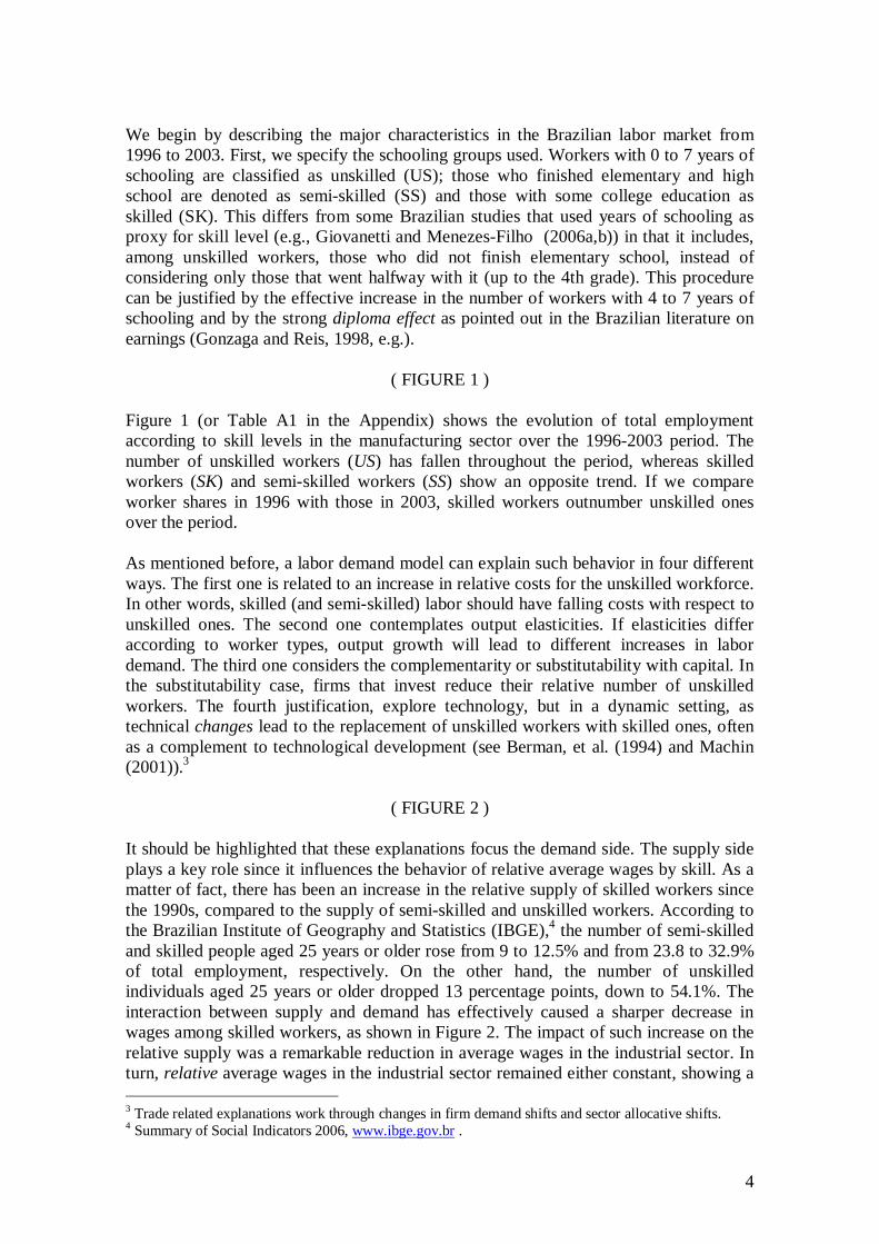
We begin by describing the major characteristics in the Brazilian labor market from 1996 to 2003. First, we specify the schooling groups used. Workers with 0 to 7 years of schooling are classified as unskilled (US); those who finished elementary and high school are denoted as semi-skilled (SS) and those with some college education as skilled (SK). This differs from some Brazilian studies that used years of schooling as proxy for skill level (e.g., Giovanetti and Menezes-Filho (2006a,b)) in that it includes, among unskilled workers, those who did not finish elementary school, instead of considering only those that went halfway with it (up to the 4th grade). This procedure can be justified by the effective increase in the number of workers with 4 to 7 years of schooling and by the strong diploma effect as pointed out in the Brazilian literature on earnings (Gonzaga and Reis, 1998, e.g.).

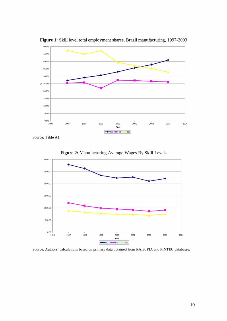
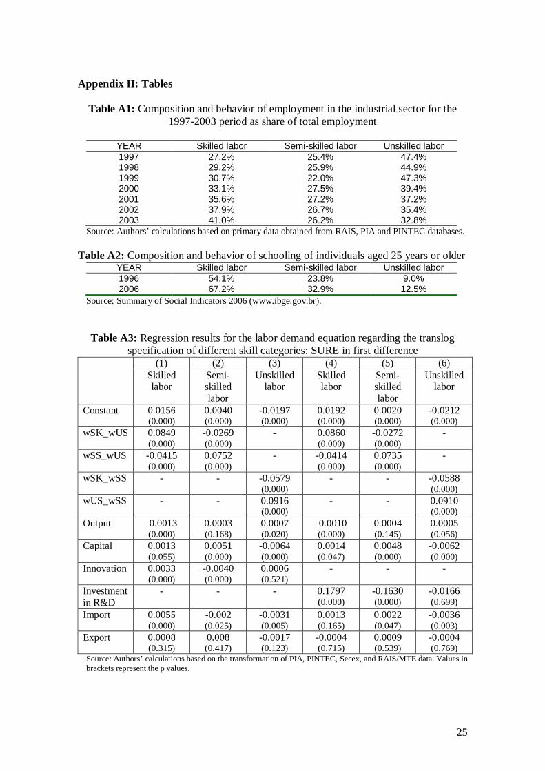
( FIGURE 1 ) Figure 1 (or Table A1 in the Appendix) shows the evolution of total employment according to skill levels in the manufacturing sector over the 1996-2003 period. The number of unskilled workers (US) has fallen throughout the period, whereas skilled workers (SK) and semi-skilled workers (SS) show an opposite trend. If we compare worker shares in 1996 with those in 2003, skilled workers outnumber unskilled ones over the period. As mentioned before, a labor demand model can explain such behavior in four different ways. The first one is related to an increase in relative costs for the unskilled workforce. In other words, skilled (and semi-skilled) labor should have falling costs with respect to unskilled ones. The second one contemplates output elasticities. If elasticities differ according to worker types, output growth will lead to different increases in labor demand. The third one considers the complementarity or substitutability with capital. In the substitutability case, firms that invest reduce their relative number of unskilled workers. The fourth justification, explore technology, but in a dynamic setting, as technical changes lead to the replacement of unskilled workers with skilled ones, often as a complement to technological development (see Berman, et al. (1994) and Machin (2001)).3

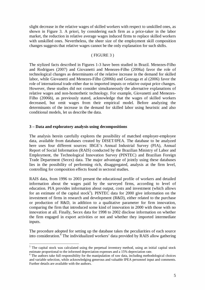
( FIGURE 2 ) It should be highlighted that these explanations focus the demand side. The supply side plays a key role since it influences the behavior of relative average wages by skill. As a matter of fact, there has been an increase in the relative supply of skilled workers since the 1990s, compared to the supply of semi-skilled and unskilled workers. According to the Brazilian Institute of Geography and Statistics (IBGE),4 the number of semi-skilled and skilled people aged 25 years or older rose from 9 to 12.5% and from 23.8 to 32.9% of total employment, respectively. On the other hand, the number of unskilled individuals aged 25 years or older dropped 13 percentage points, down to 54.1%. The interaction between supply and demand has effectively caused a sharper decrease in wages among skilled workers, as shown in Figure 2. The impact of such increase on the relative supply was a remarkable reduction in average wages in the industrial sector. In turn, relative average wages in the industrial sector remained either constant, showing a 3 Trade related explanations work through changes in firm demand shifts and sector allocative shifts. 4 Summary of Social Indicators 2006, www.ibge.gov.br .

5

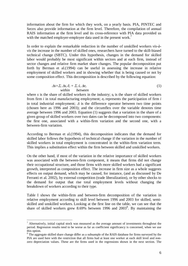
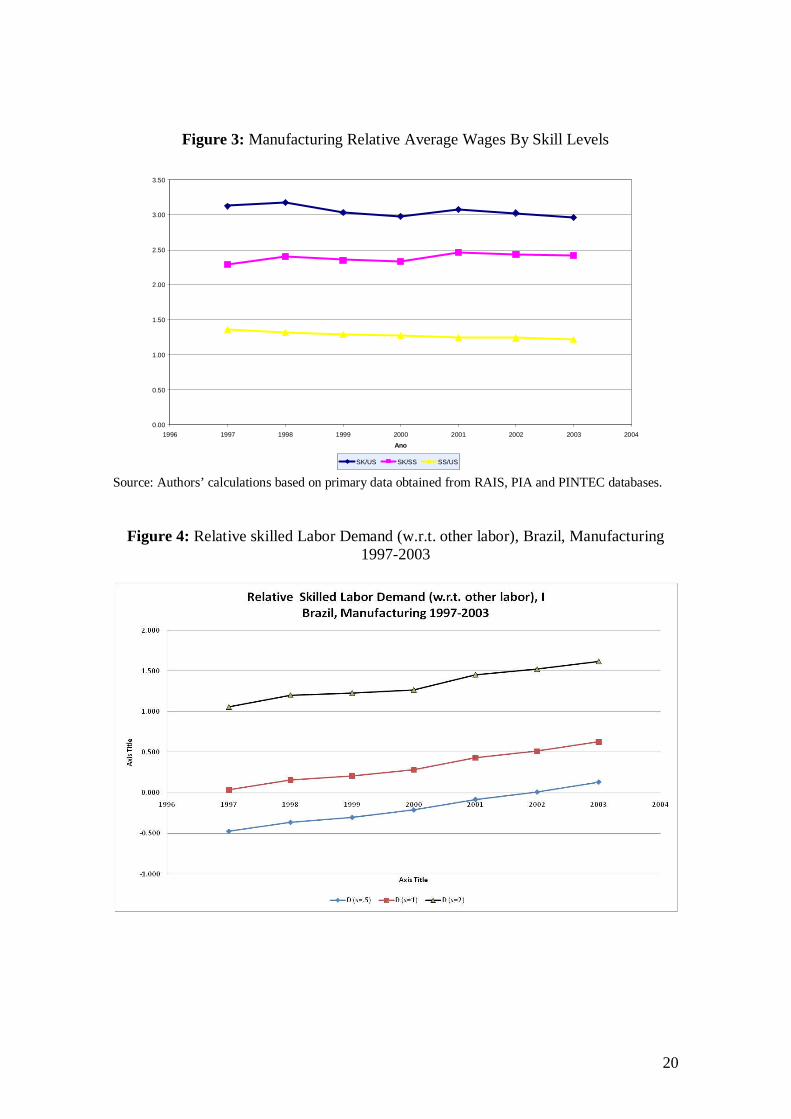
slight decrease in the relative wages of skilled workers with respect to unskilled ones, as shown in Figure 3. A priori, by considering each firm as a price-taker in the labor market, the reduction in relative average wages induced firms to replace skilled workers with unskilled ones. Nevertheless, the sheer size of the employment skill composition changes suggests that relative wages cannot be the only explanation for such shifts.

( FIGURE 3 ) The stylized facts described in Figures 1-3 have been studied in Brazil. Menezes-Filho and Rodrigues (2007) and Giovanetti and Menezes-Filho (2006a) favor the role of technological changes as determinants of the relative increase in the demand for skilled labor, while Giovanetti and Menezes-Filho (2006b) and Gonzaga et al (2006) favor the role of international trade either due to imported imputs or relative output price changes. However, these studies did not consider simultaneously the alternative explanations of relative wages and non-homothetic technology. For example, Giovanetti and Menezes-Filho (2006b), as previously stated, acknowledge that the wages of skilled workers decreased, but omit wages from their empirical model. Before analyzing the determinants of the increase in the demand for skilled labor using heuristic and also conditional models, let us describe the data. 3 – Data and exploratory analysis using decompositions The analysis herein carefully explores the possibility of matched employer-employee data, available from databases created by DISET/IPEA. The database to be analyzed here uses four different sources: IBGE’s Annual Industrial Survey (PIA), Annual Report of Social Information (RAIS) conducted by the Brazilian Ministry of Labor and Employment, the Technological Innovation Survey (PINTEC) and Brazilian Foreign Trade Department (Secex) data. The major advantage of jointly using these databases lies in the possibility of performing rich, disaggregated, analysis at the firm level, controlling for composition effects found in sectoral studies. RAIS data, from 1996 to 2003 present the educational profile of workers and detailed information about the wages paid by the surveyed firms, according to level of education. PIA provides information about output, costs and investment (which allows for an estimate of the capital stock5). PINTEC data for 2000 give information on the investment of firms in research and development (R&D), either related to the purchase or production of R&D, in addition to a qualitative parameter for firm innovation, comparing the firm that introduced some kind of innovation in 2000 with those with no innovation at all. Finally, Secex data for 1998 to 2002 disclose information on whether the firm engaged in export activities or not and whether they imported intermediate inputs. The procedure adopted for setting up the database takes the peculiarities of each source into consideration.6 The individualized workers’ data provided by RAIS allow gathering

5 The capital stock was calculated using the perpetual inventory method, using an initial capital stock estimate proportional to the informed depreciation expenses and a 15% depreciation rate. 6 The authors take full responsibility for the manipulation of raw data, including methodological choices and variable selection, while acknowledging generous and valuable IPEA personnel input and comments. Further details are available with the authors.

6

information about the firm for which they work, on a yearly basis. PIA, PINTEC and Secex also provide information at the firm level. Therefore, the compilation of annual RAIS information at the firm level and its cross-reference with PIA data provided us with the matched employer-employee data used in the present work.7 In order to explain the remarkable reduction in the number of unskilled workers vis-à-vis the increase in the number of skilled ones, researchers have turned to the skill-biased technical change (SBTC). Under this hypothesis, changes in the demand for skilled labor would probably be most significant within sectors and at each firm, instead of sector changes and relative firm market share changes. The popular decomposition put forth by Berman et al.(1994) can be useful in assessing the increase in relative employment of skilled workers and in showing whether that is being caused or not by some composition effect. This decomposition is described by the following equation:

∆s=Σi ∆si êi + Σi ŝi ∆ei (1)

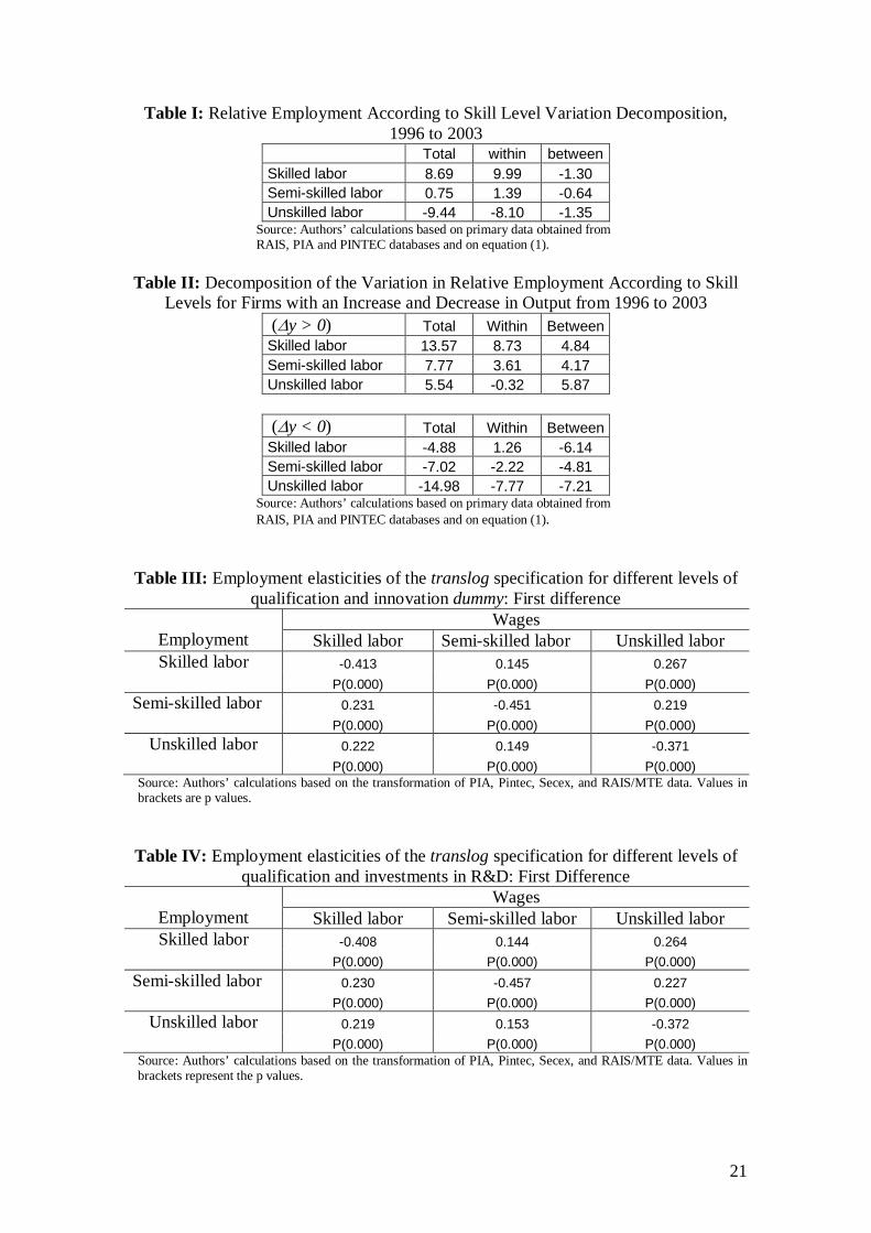
within between where s is the share of skilled workers in the industry; si is the share of skilled workers from firm i in total manufacturing employment; ei represents the participation of firm i in total industrial employment; ∆ is the difference operator between two time points (chosen here as 1996 and 2003); and the circumflex over the variable denotes time average between 1996 and 2003. Equation (1) suggests that a variation in the share of a given group of skilled workers over two dates can be decomposed into two components: the first one, associated with a within-firm variation and the second one, with a between-firm variation. According to Berman et al.(1994), this decomposition indicates that the demand for skilled labor follows the hypothesis of technical change if the variation in the number of skilled workers in total employment is concentrated in the within-firm variation term. This implies a substitution effect within the firm between skilled and unskilled workers. On the other hand, if most of the variation in the relative importance of skilled workers was associated with the between-firm component, it means that firms did not change their occupational structure, and those firms with more skilled workers had a significant growth, interpreted as composition effect. The increase in firm size as a whole suggests effects on output demand, which may be caused, for instance, (and as discussed by De Ferranti et al. 2002), by external competition (trade liberalization), or by other shocks to the demand for output that rise total employment levels without changing the breakdown of workers according to their type. Table I shows the within-firm and between-firm decomposition of the variation in relative employment according to skill level between 1996 and 2003 for skilled, semi-skilled and unskilled workers. Looking at the first line on the table, we can see that the share of skilled workers grew 8.69% between 1996 and 20038. By maintaining the

7 Alternatively, initial capital stock was measured as the average amount of investments throughout the period. Regression results tend to be worse as far as coefficient significancy is concerned, when we use this option. 8 The aggregate skilled share change differ as a subsample of the RAIS database for firms surveyed by the PIA are used here with the restriction that all firms had at least one worker at each skill level and non-zero depreciation values. These are the firms used in the regressions shown in the next section. The

7

relative importance of each firm in total employment constant, the within-firm term of the decomposition indicates that the number of skilled workers in total employment increased by nearly 10%. Finally, firms that employed more skilled workers reduced their share in total employment, as seen by the negative between-firm variation of -1.30%. The importance of the within-firm component for skilled workers in explaining the total result indicates that the composition effect was negligible and that skilled labor increased mainly with the replacement of workers at the firms. For semi-skilled workers, variation in total employment was also positive, but negligible (0.75%). This variation, just as in the case of skilled workers, resulted to a great extent from the increase in the number of semi-skilled workers at each firm (1.39%), as firm share shifts led a -0.64% decrease in semiskilled workers in total employment. As expected9, the relative number of unskilled workers fell -9.44% between 1996 and 2003. Most of this decrease occurred due to within-firm variations, whose magnitude was -8.10. The between-firm effect amplified this decrease, with a negative variation of -1.35%.

( TABLE I ) These results for the three types of workers show that the increase in the number of skilled workers (and the decrease in relative employment of unskilled workers) occurred within firms, suggesting that the SBTC could be held accountable for the increase in the participation of skilled workers. This result is not new, as evidence in favor of this hypothesis was obtained, for instance, by Menezes-Filho and Rodrigues (2003). A limitation regarding the interpretation of the importance of the within-firm effect as an indicator that technical progress is the major reason for the increase in skilled labor is the lack of control over other sources of employment changes in each firm. As stated above, there are specific factors to each firm that may justify the relative increase in skilled labor, such as capital-labor complementarity (Hamermesh, 1993) and non-homothetic technology (Sosin and Farichild, 1984). For a preliminary separation of the effects of changes in demand, which are specific to each firm, we propose an extension to the decomposition above, in which firms are grouped according to output behavior. Therefore, we have a group of firms that had an increase in their output (denoted by G) and another group of firms that experienced a decrease in their value added (denoted by D). In mathematical terms, equation (1) is rewritten as:

∆s= (Σi∈G ∆si êi +Σi∈D ∆si êi) + (Σi∈G ŝi ∆ei + Σi∈D ŝi ∆ei) (1’) within between

where G={i=1,..., n |∆yi>0} and D={i=1,..., n |∆yi≤0} are respectively the group of firms with an increase in their value added at constant prices (y) and the group of firms with a decrease (non-increase) in their real value added. The equation above can be

qualitative results of the decompositions, which are available from the authors, do not change if the total sample is used. 9 A careful reader may note that the vertical sum of the TOTAL column values should be zero, as we work with changes in the relative number of workers according to skill level, in the economy as a whole. This is not necessary for the within and between columns, individually.

8

rearranged to isolate effects for those firms that increase and for those that decrease their real value added10

∆s=∆sG+∆sD = [Σi∈G ∆si êi + Σi∈G ŝi ∆ei] +[ Σi∈D ∆si êi + Σi∈D ŝi ∆ei] (2) within between within between

output growth output decrease

Table II shows decomposition (2). The upper part of the table shows the results for the firms with an increase in output while the lower part shows the results for the firms with a decrease in their value added. As expected, employment falls at all skill levels when output varies negatively, since theoretically we expect a positive output elasticity. Nevertheless, the differences in the magnitude of changes are quite evident. In the lower part of the table, the decrease in skilled labor is almost three times lower than that for unskilled labor. The -4.88% reduction in total employment in the group of skilled workers can be attributed to the changes in firm sizes (composition effect), since within-firm variation was positive (1.26%). For unskilled workers, the decomposition shows that nearly 50% of the reduction was due to within-firm variations (7.77%), whereas the remaining 7.21% was due to between-firm variations. This result indicates the possibility for non-homogeneous output elasticities across the different types of workers. This remains true when we assess firms that experienced output growth, by having a look at the upper part of the table: the increase in the relative number of skilled workers was larger than in that of unskilled ones and this increase occurred chiefly within firms. The between-firm effect is similar across all schooling groups.

( TABLE II )

In general, Table II results show different firm behaviors. Unskilled workers are more severely affected by negative shocks to profitability, whereas skilled workers benefit from positive shocks, indicating a strong substitution effect. This effect may result from different output elasticities across the groups of workers. The alternative explanation of the SBTC can also be valid, provided that the firms which increased their value added were those which invested more heavily in technology. That is, the results above become more relevant when we gather evidence that the demand for skilled workers also responds to variations in output, suggesting that technological changes causing the demand for skilled labor to increase may account for only a part of the variations in this demand. Another popular decomposition in the skill upgrade literature was proposed by Katz and Murphy (1992). It estimates the extent of skilled labor demand shifts under constant returns to scale CES technology and competitive markets assumptions. It is based on the following decomposition for demand shifts D,

D=ln(wi/wj) + σ-1ln(Li/Lj)

10 Value added is measured by the value of industrial transformation, deflated by the general price index (GPI) of the sector, and if it is not available, by the average GPI, obtained from PIA We thank the technical staff of DISET/IPEA for suggestions regarding GPI calculations and data.

9

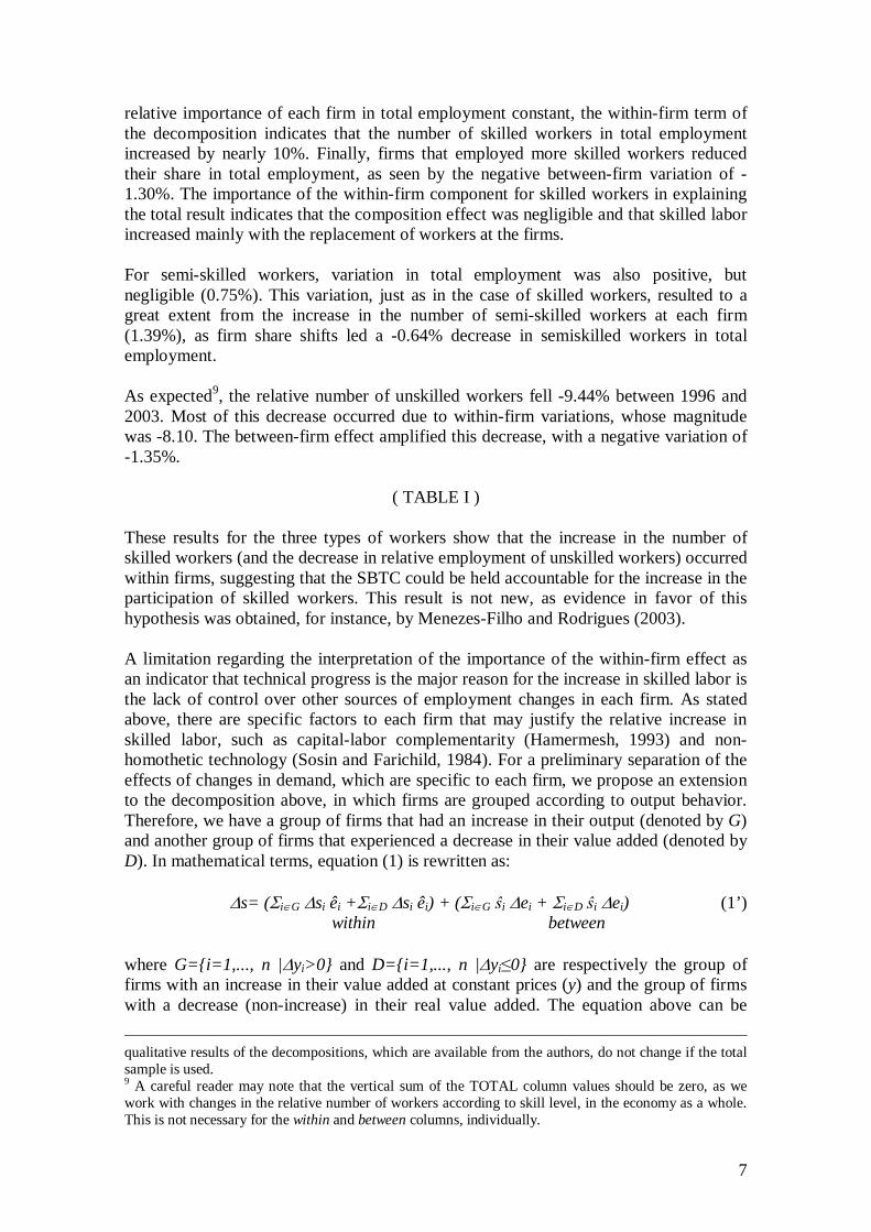
Where i,j=sk, ss, us and s is the elasticity of substitution between any two types of labor. Figure 4 present these demand shifts under alternative hypothesis on the elasticity of substitution. In all cases, there seem to be positive and stronger demand shifts. While this is interpreted as indirect evidence of technological changes, consider Sosin and Fairchild (1984) non homothetic, technological change non-neutral CES output function, simplified for two inputs only,

A[ Yβ1 (ESK LSK)- ρ + Yβ2 (EUS LUS)

- ρ] 1/ ρ -1 =0 where ESK and EUS are labor efficiency shifters, A is Hicks-neutral technical change and β1 and β2 are non-homotheticity parameters. Technical progress is measured by shifts in the efficiency shifters. Under competitive labor markets, the labor demand function yields the following expression for the demand shifter defined above

D = ρ ln(EU/ES) + σ(β1 – β2)lnY

It is easy to see that the demand shift depends on both technical progress (changes in EUS/ESK) and output changes with non-homothetic technology (β1 – β2 ≠0).

( FIGURE 4 ) The results of decompositions suggest, just as in other studies, that the increase in skilled labor occurred within firms and was not determined by a relative change in the importance of firms that employ more skilled workers. The same results also suggest that technological change could not be the only, or at least, the major cause for this relative increase in skilled labor in Brazil between 1996 and 2003. Other effects, such as variations in output, should be further investigated. This type of analysis will be carried out in the subsequent sections with the specification of flexible functional form labor demand models. 4- Labor demand model Our empirical model follows a standard labor demand model by skill type (Hamermesh, 1993), assuming cost minimization in a static choice problem (or with high costs for intertemporal adjustments) and a variable cost function in which capital is assumed as fixed (or separable) input. The production function and the associated labor demand functional form must include factors related to technological progress, potentially nonneutral in the sense of Hicks and be general enough not to impose separability and/or homotheticity (Machin, 2001, Baltagi and Rich, 2005, among others). We considered two functional forms, the Translog, which has been often used due to its flexibility ( e.g., Berndt, 1991) and the Generalized Leontief (GL), as in Chan and Rich (2006). The popular yet restrictive log-linear model was analyzed as it imposes homotheticity, unity elasticity of substitution and constant was elasticities. Our empirical results on the Translog always reject these restrictions. The GL model yielded non-significant coefficients everywhere, so its results are relegated to the Appendix.

10

Following Berndt, 1991, the translog functional form can be understood as a second-order approximation for a cost function with unknown technology. Due to the difficulty in setting up individual measures of capital cost, we consider capital as a quasi-fixed input and the translog function explains the variable costs. As the analysis focuses on employment, the output measure should be value added, which excludes the costs of materials. Thus, by omitting an indicator for firm j, the functional form of the variable cost function is:

Ln VC = α0 + αy ln Y + αk ln K + Σi γi ln wi + αz Z + ½ αyy (lnY)2+ ½ αkk (lnK)2+ ½ αyk lnY lnK + ½ αzz (Z)2+ ½ αzy Z lnY + ½ αzk Z ln K (4) + ½ΣiΣjγij lnwi

lnwj +½ Σiαiy lnwi lnY

+½ ΣiαiK lnwi lnK+½ Σiαiz lnwi Z where VC represents the variable costs, Y is the output (value added), K is the capital stock, wi is the price of i=1,.., n variable inputs, Z is a proxy for technology (which may be a linear trend or time dummies). Some restrictions can be imposed on the coefficients so that they are consistent with the theoretical hypotheses, such as homogeneity of degree one in input prices (Σiγi=1, Σiγij =Σjγij = Σiγiy =0) and symmetry of price effects (γij=γji) or constitute special cases of this cost function, such as homotheticity (if αiy=0 ∀ i), homogeneity of degree g (γyy=0), and neutrality of the technological progress (αiz=0 ∀ i). Even though the translog form cannot be used to directly calculate labor demand equations, the wage elasticities, output elasticities, and cross elasticities can be calculated based on a system of equations obtained from Shephard’s lemma, which produces equations for the share Si of the variable cost of inputs i: ∂ ln VC = ∂ VC /VC = Pi Xi = γi + Σjγij lnwi + αιy ln Y + αik ln K + αiz Z (5) ∂ ln wi ∂ wi / wi C

Our model consider three employment categories (skilled labor – sk; semi-skilled labor –ss; and unskilled labor - us), generating the following system of equations: Ssk = γsk + γsk,sk ln(wsk/wus) + γsk,ss ln(wss/wus) + αsk,y ln y + αsk,z Z (6) Sss = γss + γss,sk ln(wsk/wus) + γss,ss ln(wss/wus) + αss,y ln y + αss,z Z

Unskilled workers cost share equation was omitted due to the restriction that the sum of labor cost shares in variable costs is constant and equal to 1. The coefficients that are not estimated can be obtained using the theoretical restrictions, namely:

γsk,ss =γss,sk

γus,sk =γsk,us = – (γsk,sk + γsk,ss) γus,ss =γss,us = – (γss,sk + γss,ss) (7) γus,us =– (γus,sk + γus,ss) = γsk,sk + γss,ss + 2γsk,ss.

Wage elasticities and cross-wage elasticities (or elasticities of substitution and complementarity) are calculated by:

11

εsk,sk = γsk,sk/Ssk + (Ssk – 1) εsk,ss = γsk,ss/Ssk + Sss εsk,us = γsk,us/Ssk + Sus

εss,sk = γss,sk/Sss + Ssk εss,ss = γsk,ss/Sss + (Sss – 1) εss,us = γss,us/Sss + Sus (8)

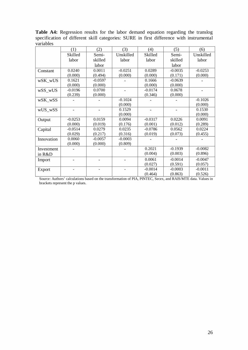
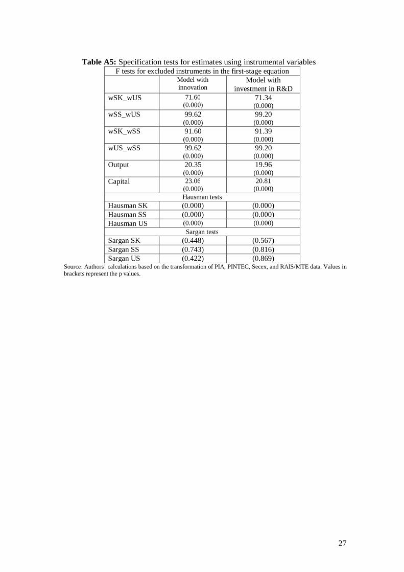
εus,sk = γus,sk/Sus + Sus εus,ss = γus,ss/Sus + Sss εus,us = γus,us/Sus + (Ssk – 1) Before the estimations, some comments are necessary. Wage elasticities are expected to have a negative sign and to be decreasing as skill level rises. In turn, the cross-wage elasticities (or elasticities of substitution) may have either a negative or positive sign, depending on whether the groups of workers are complements or substitutes between themselves. Technical or organizational changes should have a significant impact on the group of unskilled workers. Therefore, if technology is non-homothetic, an increase in output changes the input use ratio or the intensity of the use of the capital factor. To identify the hypothesis of non-homotheticity, we will first verify whether output (or capital) affects the demand for skilled labor (coefficients αi,y and αi,z significance). After that, to check whether output is responsible for the relative increase in the number of skilled workers compared to that of unskilled workers, we test the difference of output elasticities among the types of workers (i.e., test of αsk,y –αus,y = 0, for skilled and unskilled labor). Similarly, the test can be run for the capital effect (αsk,K–αus,K = 0).11 To complete the explanatory variables set, we proxy for technology (variable Z) using a dummy for firms that innovate and R&D expenditures as share or value added (both from PINTEC). In addition, we use year dummies to capture the effects of the SBTC, as in Baltagi and Rich (2005). Last, we control for international trade effects by a dummy for the year that a firm exports and imports, both from (Secex). The inclusion of these variables contemplates two alternative explanations to the downward shift of the demand for unskilled workers. As technology is measured through proxies, we assessed the robustness of results by using different proxies. Further analysis of trade liberalization effects are not warranted as the main thrust of tariff and non-tariff barrier reductions was in during the 1988-1998 period (Gonzaga et al., 2006). The specification is completed with the assumption of unobserved firm specific fixed effects. The estimation uses the standard method for this type of literature - seemingly unrelated regression estimation (SURE) - with first-difference variables except for the variables obtained from PINTEC (investment in R&D and dummy for the innovative firm) in the level, since the available information corresponds only to the year 2000. The major justification for this procedure is based on the fact that investment in R&D measures the (average) flow of investment in knowledge by the firm, representing the variation in the technology stock of a firm.12 We tackle the possible measurement errors and the endogeneity between wages and output, using instrumental variables (second and third lags for wage, output and capital).

11 Note that it is not possible to obtain output (or capital) elasticities from the estimation of system (6), since the system does not estimate coefficients αy and αyy. However, it is possible to assess the difference of output elasticities across the types of workers, as they involve the estimated αi,y coefficients. 12 In addition, according to the PINTEC database, the information corresponds to the average expenditure for the 1999-2001 period.

12

5- Estimates of employment-wage elasticities and employment-output for Brazilian manufacturing Estimation of the system (6) above produces a large number of parameters that must be transformed in order to yield elasticities. To make the presentation easier, we focus the analysis on elasticities and relegate the complete set of coefficient estimates to the Appendix. As mentioned before, based on previous results reported in the literature, the signs of the wage elasticities are expected to be negative and the magnitude is expected to be smaller, the higher the skill level, whereas for cross-wage elasticity, the sign can be either positive or negative, indicating whether the types of labor are substitutes or complements. The elasticities generated by the Generalized Leontief are shown in the Appendix, for robustness sake documentation, as the results obtained were mostly insignificant and theoretically inconsistent. The results are presented for the different proxies for technological change, and using or not instrumental variables. Table III shows the elasticities obtained from the SURE procedure for system (6), omitting the equation for unskilled workers.13 The main diagonal provides the wage elasticities for the category being estimated, whereas outside the main diagonal, we have the cross-wage elasticity. The signs of the wage elasticities are as expected, statistically significant, and inelastic. The demand for semi-skilled workers is more elastic than for the other types of workers. The signs of the cross-wage elasticities indicate that skilled workers replace semi-skilled or unskilled workers and vice versa. Alos, semi-skilled and unskilled workers are substitutes in production.

( TABLE III ) Table IV shows the elasticities obtained for the same system of equations, but with the use of investment in R&D variable in lieu of the innovation dummy, in addition to dummies for importing and exporting activity in order to capture international trade activity (see the regression results in the Appendix). The specification changes impact on elasticities is small, usually to the second decimal place. Tables III and IV show that wage elasticities decrease in absolute values for semi-skilled workers. This result suggests that there exists some hierarchy between wage elasticities when we analyze demand for skilled labor, which is different from the one expected and described in Hamermesh (1993), Robert and Skoufias (1997), FitzRoy and Funke (1998), among others – although, in general, these studies used two types of workers. However, this result is similar to the one obtained by Addison et al. (2005) when assessing the demand for skilled labor in Germany.

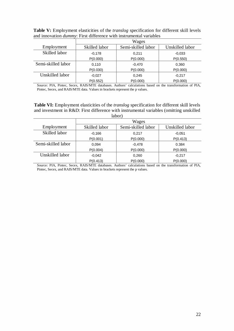
( TABLE IV ) Table V presents the results for the same specifications above, but using instrumental variables. The major changes are associated with skilled workers’ elasticities. First, elasticities decrease in terms of absolute value, getting to (statistically) zero in case of cross-wage elasticity between skilled and unskilled workers. Since wage elasticities for

13 The results are qualitatively the same and change very slightly in quantitative terms when we estimate system (6) by omitting the equation for semi-skilled workers instead of excluding the equation for unskilled workers.

13

semi-skilled and unskilled workers change slightly, these workers are replaced at a higher frequency, as cross-wage elasticities are higher.

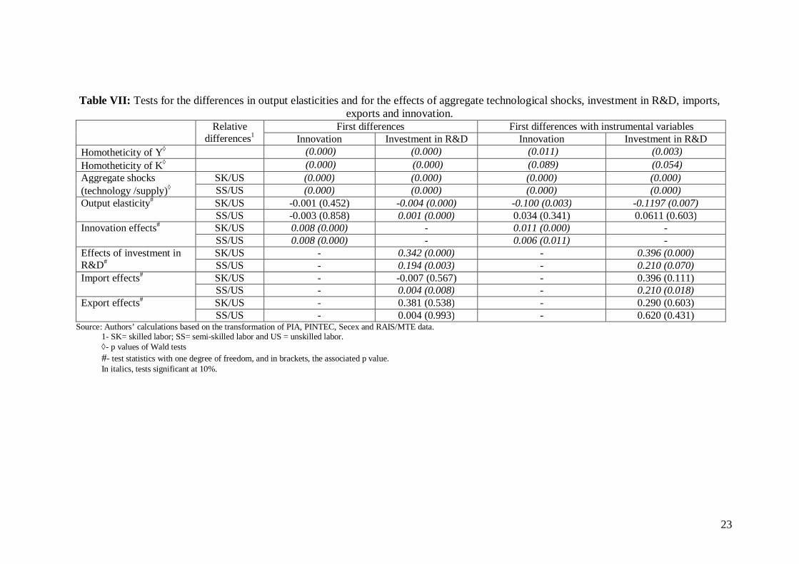
( TABLE V ) By comparing Tables V and VI, which use different proxies for technology, we note that this has a negligible influence on results. However, the significance of the wage elasticities in Tables V and VI makes it clear that the simplification advocated by Machin et al. (1998) of omitting wage variables due to identification problems is not justifiable, at least not for the Brazilian case. Table VII shows the results for homotheticity, capital-skill level complementarity, and non-neutral technical change tests. The hypothesis of homotheticity is tested for value added and for capital, considering the joint significance of coefficients αi,y and αi,k,

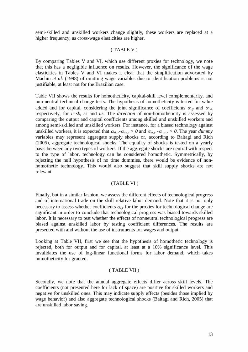
respectively, for i=sk, ss and us. The direction of non-homotheticity is assessed by comparing the output and capital coefficients among skilled and unskilled workers and among semi-skilled and unskilled workers. For instance, for a biased technology against unskilled workers, it is expected that αsk,y-αus,y > 0 and αss,y -α us,y > 0. The year dummy variables may represent aggregate supply shocks or, according to Baltagi and Rich (2005), aggregate technological shocks. The equality of shocks is tested on a yearly basis between any two types of workers. If the aggregate shocks are neutral with respect to the type of labor, technology can be considered homothetic. Symmetrically, by rejecting the null hypothesis of no time dummies, there would be evidence of non-homothetic technology. This would also suggest that skill supply shocks are not relevant.

(TABLE VI ) Finally, but in a similar fashion, we assess the different effects of technological progress and of international trade on the skill relative labor demand. Note that it is not only necessary to assess whether coefficients αi,z for the proxies for technological change are significant in order to conclude that technological progress was biased towards skilled labor. It is necessary to test whether the effects of nonneutral technological progress are biased against unskilled labor by testing coefficient differences. The results are presented with and without the use of instruments for wages and output. Looking at Table VII, first we see that the hypothesis of homothetic technology is rejected, both for output and for capital, at least at a 10% significance level. This invalidates the use of log-linear functional forms for labor demand, which takes homotheticity for granted.

( TABLE VII ) Secondly, we note that the annual aggregate effects differ across skill levels. The coefficients (not presented here for lack of space) are positive for skilled workers and negative for unskilled ones. This may indicate supply effects (besides those implied by wage behavior) and also aggregate technological shocks (Baltagi and Rich, 2005) that are unskilled labor saving.

14

Thirdly, with regard to the differences in output coefficients according to the skill category, the results depend on the controls used and on the estimation method. Using instrumental variables and investment in R&D as proxy for technological progress, we note that differences are significant only for the difference between skilled and unskilled workers (sk and us, respectively). There are no significant differences between output elasticities for semi-skilled and unskilled workers (ss and us, respectively). Surprisingly, the difference in output elasticity is against skilled labor. In other words, output growth, ceteris paribus, would cause a decrease in the number of skilled workers relative to unskilled ones. This can be confirmed by the output coefficients in Table A3 (columns (4) and (6)). Table A3 also shows that the increase in capital stock would have the same effect decreasing in the share of skilled workers. Note that the effect on the unskilled workers is zero. Fourthly, to assess the possibility of nonneutral technical change biased against unskilled labor, two proxies for technical progress were used: if the firm shows product or process innovation and R&D intensity. The tests shown in Table VII indicate that technological progress is biased against skilled labor. In addition, the coefficients in Table A3 (and A2) show that technological progress is nonneutral, as obtained by Giovanetti and Menezes-Filho (2006a,b) for Brazil. Finally, with regard to qualitative variables for international trade activity (export and import dummies), the test results suggest that the effects are not significant, except for imports, whose results indicate that importing firms proportionately employ more skilled workers. This is similar to Giovanetti and Menezes-Filho (2006b). Based on these results, it is not possible to assert that an exporting firm requires more skilled labor. However, the limited quality of the proxy (a dummy), used here for control instead of as the focus of analysis, should be considered. In sum, although technology is non-homothetic and technological progress is nonneutral, the bias against unskilled labor lies in technical progress (as measured by our innovation proxy). Given the technology identified by the model, increases in output may cause a decrease in the number of skilled workers, ceteris paribus. By looking at the effective increase in skilled labor, two factors predominate: the behavior of relative wages, influenced by shocks to the supply of skilled workers, and technological progress. Final remarks One of the major changes observed in the Brazilian labor market in the past few years has been the increase in the share of skilled workers, with a concomitant decrease in the number of unskilled workers. The present paper sought to amass new evidence regarding the factors behind this movement, focusing on the manufacturing industry, considering the possibility of nonneutral (non-homothetic) technology and the impact of relative price changes, in addition to the well-known hypotheses of nonneutral technical change (de Ferranti et al, 2002) and trade liberalization (Giovanetti and Menezes-Filho 2006b, Gonzaga et al., 2007). Note that unlike the analysis and discussion about the increase in the demand for skilled workers in the U.S., the 1996-2003 period was characterized by a decrease in

15

skilled/unskilled relative wages, induced by a significant shift in skilled labor supply. Yet, the magnitude of the relative wage shifts is too small to explain the skilled labor demand shift. The analysis relied on matched employer-employee data on workers and firms made available by IPEA, for the 1996-2003 period. For the first time in Brazil, we estimate wage elasticities across skill levels. Exploratory analysis using the popular decomposition proposed by Berman, et al. (1994) revealed that the increase in the share of skilled labor in total employment occurred within firms (substitution effects), instead of a change in the composition of firms (larger importance of firms with skilled workers, without any change in firms’ qualification structure). As seen in the literature, this result supports the hypothesis of a shift in the direction of technological change as a determinant of the increase in the number of skilled workers (e.g., Giovanetti and Menezes-Filho, 2006a). Nevertheless, this is not compatible with other firm specific demand shifts, such as wage elasticities or non-homothetic technology. However, when assessing whether this variation in the number of skilled workers was different in firms which increased and decreased their value added, we obtained evidence that the demand for skilled workers also accounts for different variations in output. In other words, technological changes that induce an increase in the demand for skilled labor may account for just some part of the variation in this demand. Using another common descriptive device for skill demand shifts, namely the Katz and Murphy (1992), CES technology demand decomposition, we confirm that there were positive demand shifts over the period, beyond what would be expect due to relative wage shifts. Nevertheless, under non-homothetic technology, it is possible to show –and has been overlooked by previous researchers – that the decomposition demand shifts can be justified with non-homothetic output growth, in addition to the usual technical progress argument. Hence, for more consistent conclusions, we estimate a labor demand function with a flexible technology and technical progress and trade related variables to sort out the conflicting hypotheses. The evidence from the econometric analysis showed that skilled and semi-skilled workers are substitutes, whereas skilled and unskilled workers may or may not be substitutes. The wage elasticities of semi-skilled workers are more elastic than all the others. Tests for non-homotheticity clearly show that technology is non-homothetic (as first suggested by Sosin and Fairchild (1984), suggesting that simple functional forms, such as the log-linear, should not be used to model manufacturing labor demand. On the other hand, technology does not seem biased against unskilled workers. The proxies for technological innovation yielded coefficients that confirmed the results obtained by other studies regarding biased technological progress in favor of skilled labor. Internation trade effects, measured by our proxies of imported input use and export activity did not come as relevant to explain labor demand shifts by skill, except for semi-skilled effects of imported inputs, as in Giovanetti and Menezes-Filho(2006b). The results of this paper allow drawing preliminary policy implications. First, given the increasing innovation pace and public policy support in Brazil (the latest industrial policy unveiled in 2004 and 2008 focus specifically on innovation), the demand for unskilled labor should decline, or at least, stagnate. Secondly, if the tendency towards

16

the increase in the supply of skilled workers persists, with reductions in relative wages as net effect of the interaction between supply and demand, firms will likely prefer skilled workers to the detriment of unskilled ones. This may create a growth-inequality trade-off, as poorer workers could face higher unemployment rates. Training policies could be targeted to reduce the relative supply of unskilled workers, increasing their wages. This is certainly an issue for further study.

17

References

Addison, J.T.; Bellmann, L.; Schank, T; Teixeira, P. 2005. The Demand for Labor: An Analysis Using Matched Employer-Employee Data from the German LIAB. Will the High Unskilled Worker Own-Wage Elasticity Please Stand Up?. Institute for the Study of Labor/IZA Discussion Paper No. 1780.

Baltagi, B.; Rich, D.P. 2005. Skill-biased technical change in US manufacturing: a general index approach. Journal of Econometrics, 126, no. 3, 529-270.

Barros, R. P.; Foguel, M. N.; Ulyssea, G. 2007. Sobre a recente queda da desigualdade de renda no Brasil. Nota Técnica. In: Barros, Ricardo Paes et all (org). Desigualdade de renda no Brasil: uma análise da queda recente, v. 1. Rio de Janeiro: IPEA.

Berman, E.; Bound, J.; Griliches, Z. 1994. Changes in the demand for skilled labor within U.S. manufacturing: evidence from the annual survey of manufactures. Quarterly Journal of Economics: 109, 367-397.

Berndt, E. 1991. The Practice of Econometrics: classic and contemporary. New York. Addison-Wesley.

Chan, W.H. e Rich, D.P. 2006. Occupational Labour Demand and the Source of Non-neutral Technical Change Oxford Bulletin Of Economics And Statistics: 68, no. 1, 23-42.

De Ferranti, G. et al. 2002. Closing the Gap: technology and wages in Latin America. Washington: The World Bank.

Fitzroy, F.; Funke, M. 1998. Skills, wages and employment in East and West Germany. Regional Studies: 32, no. 5, 459-467.

Giovannetti, B. C.; Menezes-Filho, N. A. 2006a. Tecnologia e a demanda por qualificação na indústria brasileira. Cap. 11. in: De Negri, João Alberto et all. Tecnologia, Exportação e Emprego. Brasília: IPEA.

Giovannetti, B. C.; Menezes-Filho, N. A. 2006b. Trade Liberalization and Demand for Skill in Brazil Economía (LACEA): 7, no.1, 1-28.

Gonzaga, G. e Reis, M. 1998 Dualidade ou não linearidade nos retornos à educação no Brasil. Revista de Econometria: 19, no. 2, 367-404.

Gonzaga, G.; Corseuil C.H. 2001. Emprego Industrial no Brasil: Análise de Curto e Longo Prazos. Revista Brasileira de Economia: 55, 4, 467-491.

Gonzaga, G.; Menezes-Filho, N. A.; Terra, C. 2006. Trade liberalization and the evolution of skill earnings differentials in Brazil. Journal of International Economics: 68, 345-367.

18

Green, E.; Dickerson, A.; Arbache, J.S. 2001. A picture of wage inequality and the allocation of labor through a period of trade liberalization: the case of Brazil. World Development: 29, no. 11, 1923-1939.

Hamermesh, D. 1993. Labor Demand. Cambridge: MIT Press.

Hammermesh, D.; Pfann, G. A. 1996. Adjustment costs in factor demand. Journal of Economic Literature: 34, no. 1, 264-1.292.

Katz, L. F.; Murphy, K. M. 1992. Changes in relative wages, 1963-1987: supply and demand factors. Quarterly Journal of Economics: 107, no. 1, 35-78.

Machin, S. 2001. The changing nature of labour demand in the new economy and skill-biased technology change. Oxford Bulletin of Economics and Statistics, 63, issue s1, 753-776.

Machin, S., Ryan, A., & Van Reenen, J. 1998. Technology and changes in skill structure: Evidence from seven OECD countries. Quarterly Journal of Economics: 113, 1215–1244.

Menezes-Filho, N. A.; Rodrigues, B. 2003. Tecnologia e demanda por qualificação na indústria brasileira. Revista Brasileira de Economia: 57, no. 3, 569-603.

Roberts, M. J.; Skoufias, E. 1997. The long-run demand for skilled and unskilled labor in Colombian manufacturing plants. The Review of Economics and Statistics: 79, no. 2, 330-334.

Sosin, K. e Fairchild, L. 1984. Nonhomotheticity and technological bias in production. Review of Economics and Statistics: 66, no. 1, 44-50.

Varian, H. R. 1992. Microeconomic analysis. New York: W.W. Norton & Company.

19

Figure 1: Skill level total employment shares, Brazil manufacturing, 1997-2003

0.0%

5.0%

10.0%

15.0%

20.0%

25.0%

30.0%

35.0%

40.0%

45.0%

50.0%

1996 1997 1998 1999 2000 2001 2002 2003 2004

Ano

%

SK SS US Source: Table A1.

Figure 2: Manufacturing Average Wages By Skill Levels

0.00

500.00

1,000.00

1,500.00

2,000.00

2,500.00

3,000.00

1996 1997 1998 1999 2000 2001 2002 2003 2004

Ano

SK SS US

Source: Authors’ calculations based on primary data obtained from RAIS, PIA and PINTEC databases.

20

Figure 3: Manufacturing Relative Average Wages By Skill Levels

0.00

0.50

1.00

1.50

2.00

2.50

3.00

3.50

1996 1997 1998 1999 2000 2001 2002 2003 2004

Ano

SK/US SK/SS SS/US

Source: Authors’ calculations based on primary data obtained from RAIS, PIA and PINTEC databases.

Figure 4: Relative skilled Labor Demand (w.r.t. other labor), Brazil, Manufacturing 1997-2003

21

Table I: Relative Employment According to Skill Level Variation Decomposition, 1996 to 2003

Total within between Skilled labor 8.69 9.99 -1.30 Semi-skilled labor 0.75 1.39 -0.64 Unskilled labor -9.44 -8.10 -1.35

Source: Authors’ calculations based on primary data obtained from RAIS, PIA and PINTEC databases and on equation (1).

Table II: Decomposition of the Variation in Relative Employment According to Skill

Levels for Firms with an Increase and Decrease in Output from 1996 to 2003 (∆y > 0) Total Within Between Skilled labor 13.57 8.73 4.84 Semi-skilled labor 7.77 3.61 4.17 Unskilled labor 5.54 -0.32 5.87

(∆y < 0) Total Within Between Skilled labor -4.88 1.26 -6.14 Semi-skilled labor -7.02 -2.22 -4.81 Unskilled labor -14.98 -7.77 -7.21

Source: Authors’ calculations based on primary data obtained from RAIS, PIA and PINTEC databases and on equation (1).

Table III: Employment elasticities of the translog specification for different levels of qualification and innovation dummy: First difference

Employment

Wages Skilled labor Semi-skilled labor Unskilled labor

Skilled labor -0.413 0.145 0.267 P(0.000) P(0.000) P(0.000)

Semi-skilled labor 0.231 -0.451 0.219 P(0.000) P(0.000) P(0.000)

Unskilled labor 0.222 0.149 -0.371 P(0.000) P(0.000) P(0.000)

Source: Authors’ calculations based on the transformation of PIA, Pintec, Secex, and RAIS/MTE data. Values in brackets are p values.

Table IV: Employment elasticities of the translog specification for different levels of qualification and investments in R&D: First Difference

Employment

Wages Skilled labor Semi-skilled labor Unskilled labor

Skilled labor -0.408 0.144 0.264 P(0.000) P(0.000) P(0.000)

Semi-skilled labor 0.230 -0.457 0.227 P(0.000) P(0.000) P(0.000)

Unskilled labor 0.219 0.153 -0.372 P(0.000) P(0.000) P(0.000)

Source: Authors’ calculations based on the transformation of PIA, Pintec, Secex, and RAIS/MTE data. Values in brackets represent the p values.

22

Table V: Employment elasticities of the translog specification for different skill levels and innovation dummy: First difference with instrumental variables

Employment Wages

Skilled labor Semi-skilled labor Unskilled labor Skilled labor -0,178 0,211 -0,033

P(0.000) P(0.000) P(0.550)

Semi-skilled labor 0,110 -0,470 0,360 P(0.030) P(0.000) P(0.000)

Unskilled labor -0,027 0,245 -0,217 P(0.552) P(0.000) P(0.000)

Source: PIA, Pintec, Secex, RAIS/MTE databases. Authors’ calculations based on the transformation of PIA, Pintec, Secex, and RAIS/MTE data. Values in brackets represent the p values.

Table VI: Employment elasticities of the translog specification for different skill levels and investment in R&D: First difference with instrumental variables (omitting unskilled

labor)

Employment Wages

Skilled labor Semi-skilled labor Unskilled labor Skilled labor -0,166 0,217 -0,051

P(0.001) P(0.000) P(0.413)

Semi-skilled labor 0,094 -0,478 0.384 P(0.004) P(0.000) P(0.000)

Unskilled labor -0,042 0,260 -0,217 P(0.413) P(0.000) P(0.000)

Source: PIA, Pintec, Secex, RAIS/MTE databases. Authors’ calculations based on the transformation of PIA, Pintec, Secex, and RAIS/MTE data. Values in brackets represent the p values.

23

Table VII: Tests for the differences in output elasticities and for the effects of aggregate technological shocks, investment in R&D, imports,

exports and innovation. Relative

differences1 First differences First differences with instrumental variables

Innovation Investment in R&D Innovation Investment in R&D Homotheticity of Y◊ (0.000) (0.000) (0.011) (0.003) Homotheticity of K◊ (0.000) (0.000) (0.089) (0.054) Aggregate shocks (technology /supply)◊

SK/US (0.000) (0.000) (0.000) (0.000) SS/US (0.000) (0.000) (0.000) (0.000)

Output elasticity# SK/US -0.001 (0.452) -0.004 (0.000) -0.100 (0.003) -0.1197 (0.007) SS/US -0.003 (0.858) 0.001 (0.000) 0.034 (0.341) 0.0611 (0.603)

Innovation effects# SK/US 0.008 (0.000) - 0.011 (0.000) - SS/US 0.008 (0.000) - 0.006 (0.011) -

Effects of investment in R&D#

SK/US - 0.342 (0.000) - 0.396 (0.000) SS/US - 0.194 (0.003) - 0.210 (0.070)

Import effects# SK/US - -0.007 (0.567) - 0.396 (0.111) SS/US - 0.004 (0.008) - 0.210 (0.018)

Export effects# SK/US - 0.381 (0.538) - 0.290 (0.603) SS/US - 0.004 (0.993) - 0.620 (0.431)

Source: Authors’ calculations based on the transformation of PIA, PINTEC, Secex and RAIS/MTE data. 1- SK= skilled labor; SS= semi-skilled labor and US = unskilled labor. ◊- p values of Wald tests #- test statistics with one degree of freedom, and in brackets, the associated p value. In italics, tests significant at 10%.

24

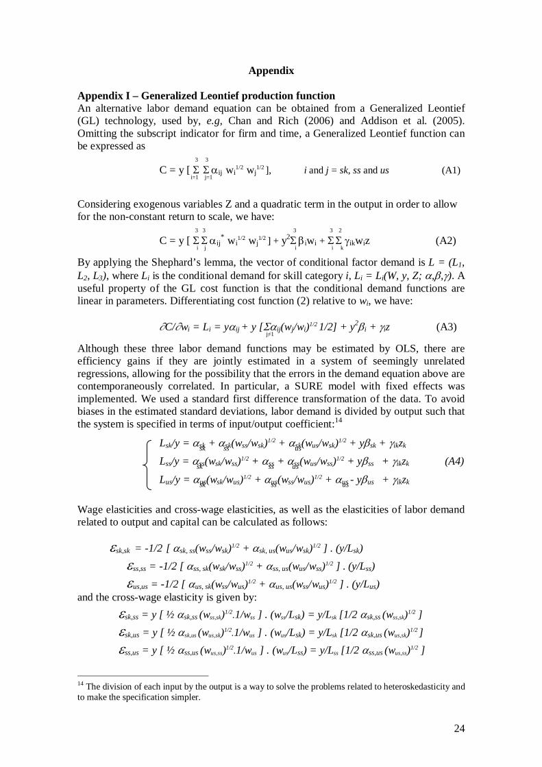
Appendix Appendix I – Generalized Leontief production function An alternative labor demand equation can be obtained from a Generalized Leontief (GL) technology, used by, e.g, Chan and Rich (2006) and Addison et al. (2005). Omitting the subscript indicator for firm and time, a Generalized Leontief function can be expressed as

3 3

C = y [ Σ Σ

αij

wi

1/2 wj1/2 ], i and j = sk, ss and us (A1)

i=1 j=1

Considering exogenous variables Z and a quadratic term in the output in order to allow for the non-constant return to scale, we have:

3 3 3 3 2

C = y [ Σ Σ

αij

* wi

1/2 wj1/2 ] + y2

Σ βiwi + Σ Σ γikwiz (A2) i j i i k

By applying the Shephard’s lemma, the vector of conditional factor demand is L = (L1, L2, L3), where Li is the conditional demand for skill category i, Li = Li(W, y, Z; α,β,γ). A useful property of the GL cost function is that the conditional demand functions are linear in parameters. Differentiating cost function (2) relative to wi, we have:

∂C/∂wi = L i = yαij + y [Σαij(wj/wi)1/2 1/2] + y2βi + γiz (A3) j≠1

Although these three labor demand functions may be estimated by OLS, there are efficiency gains if they are jointly estimated in a system of seemingly unrelated regressions, allowing for the possibility that the errors in the demand equation above are contemporaneously correlated. In particular, a SURE model with fixed effects was implemented. We used a standard first difference transformation of the data. To avoid biases in the estimated standard deviations, labor demand is divided by output such that the system is specified in terms of input/output coefficient:14

Lsk/y = αsk + αsk(wss/wsk)1/2 + αsk(wus/wsk)1/2 + yβsk + γikzk

sk ss us

Lss/y = αss(wsk/wss)1/2 + αss + αss(wus/wss)1/2 + yβss + γikzk (A4)

sk ss us

Lus/y = αus(wsk/wus)1/2 + αus(wss/wus)1/2 + αus - yβus + γikzk

sk ss us

Wage elasticities and cross-wage elasticities, as well as the elasticities of labor demand related to output and capital can be calculated as follows:

εsk,sk = -1/2 [ αsk, ss(wss/wsk)1/2 + αsk, us(wus/wsk)1/2 ] . (y/Lsk)

εss,ss = -1/2 [ αss, sk(wsk/wss)1/2 + αss, us(wus/wss)1/2 ] . (y/Lss)

εus,us = -1/2 [ αus, sk(wss/wus)1/2 + αus, us(wss/wus)1/2 ] . (y/Lus) and the cross-wage elasticity is given by:

εsk,ss = y [ ½ αsk,ss (wss,sk)1/2.1/wss ] . (wss/Lsk) = y/Lsk [1/2 αsk,ss (wss,sk)1/2 ]

εsk,us = y [ ½ αsk,us (wus,sk)1/2.1/wus ] . (wus/Lsk) = y/Lsk [1/2 αsk,us (wus,sk)1/2 ]

εss,us = y [ ½ αss,us (wus,ss)1/2.1/wus ] . (wus/Lss) = y/Lss [1/2 αss,us (wus,ss)1/2 ]

14 The division of each input by the output is a way to solve the problems related to heteroskedasticity and to make the specification simpler.

25

Appendix II: Tables

Table A1: Composition and behavior of employment in the industrial sector for the 1997-2003 period as share of total employment

YEAR Skilled labor Semi-skilled labor Unskilled labor 1997 27.2% 25.4% 47.4% 1998 29.2% 25.9% 44.9% 1999 30.7% 22.0% 47.3% 2000 33.1% 27.5% 39.4% 2001 35.6% 27.2% 37.2% 2002 37.9% 26.7% 35.4% 2003 41.0% 26.2% 32.8%

Source: Authors’ calculations based on primary data obtained from RAIS, PIA and PINTEC databases. Table A2: Composition and behavior of schooling of individuals aged 25 years or older

YEAR Skilled labor Semi-skilled labor Unskilled labor 1996 54.1% 23.8% 9.0% 2006 67.2% 32.9% 12.5%

Source: Summary of Social Indicators 2006 (www.ibge.gov.br).

Table A3: Regression results for the labor demand equation regarding the translog

specification of different skill categories: SURE in first difference (1) (2) (3) (4) (5) (6)

Skilled labor

Semi-skilled labor

Unskilled labor

Skilled labor

Semi-skilled labor

Unskilled labor

Constant 0.0156 (0.000)

0.0040 (0.000)

-0.0197 (0.000)

0.0192 (0.000)

0.0020 (0.000)

-0.0212 (0.000)

wSK_wUS 0.0849 (0.000)

-0.0269 (0.000)

- 0.0860 (0.000)

-0.0272 (0.000)

-

wSS_wUS -0.0415 (0.000)

0.0752 (0.000)

- -0.0414 (0.000)

0.0735 (0.000)

-

wSK_wSS - - -0.0579 (0.000)

- - -0.0588 (0.000)

wUS_wSS - - 0.0916 (0.000)

- - 0.0910 (0.000)

Output -0.0013 (0.000)

0.0003 (0.168)

0.0007 (0.020)

-0.0010 (0.000)

0.0004 (0.145)

0.0005 (0.056)

Capital 0.0013 (0.055)

0.0051 (0.000)

-0.0064 (0.000)

0.0014 (0.047)

0.0048 (0.000)

-0.0062 (0.000)

Innovation 0.0033 (0.000)

-0.0040 (0.000)

0.0006 (0.521)

- - -

Investment in R&D

- - - 0.1797 (0.000)

-0.1630 (0.000)

-0.0166 (0.699)

Import 0.0055 (0.000)

-0.002 (0.025)

-0.0031 (0.005)

0.0013 (0.165)

0.0022 (0.047)

-0.0036 (0.003)

Export 0.0008 (0.315)

0.008 (0.417)

-0.0017 (0.123)

-0.0004 (0.715)

0.0009 (0.539)

-0.0004 (0.769)

Source: Authors’ calculations based on the transformation of PIA, PINTEC, Secex, and RAIS/MTE data. Values in brackets represent the p values.

26

Table A4: Regression results for the labor demand equation regarding the translog specification of different skill categories: SURE in first difference with instrumental variables (1) (2) (3) (4) (5) (6)

Skilled labor

Semi-skilled labor

Unskilled labor

Skilled labor

Semi-skilled labor

Unskilled labor

Constant 0.0240 (0.000)

0.0011 (0.494)

-0.0251 (0.000)

0.0289 (0.000)

-0.0035 (0.171)

-0.0253 (0.000)

wSK_wUS 0.1621 (0.000)

-0.0597 (0.000)

- 0.1666 (0.000)

-0.0639 (0.000)

-

wSS_wUS -0.0196 (0.239)

0.0700 (0.000)

- -0.0174 (0.346)

0.0678 (0.000)

-

wSK_wSS - - -0.1024 (0.000)

- - -0.1026 (0.000)

wUS_wSS - - 0.1529 (0.000)

- - 0.1530 (0.000)

Output -0.0253 (0.000)

0.0159 (0.019)

0.0094 (0.176)

-0.0317 (0.001)

0.0226 (0.012)

0.0091 (0.289)

Capital -0.0514 (0.029)

0.0279 (0.217)

0.0235 (0.316)

-0.0786 (0.019)

0.0562 (0.073)

0.0224 (0.455)

Innovation 0.0060 (0.000)

-0.0057 (0.000)

-0.0003 (0.809)

- - -

Investment in R&D

- - - 0.2021 (0.004)

-0.1939 (0.003)

-0.0082 (0.896)

Import - - - 0.0061 (0.027)

-0.0014 (0.591)

-0.0047 (0.057)

Export - - - -0.0014 (0.464)

-0.0003 (0.863)

-0.0011 (0.526)

Source: Authors’ calculations based on the transformation of PIA, PINTEC, Secex, and RAIS/MTE data. Values in brackets represent the p values.

27

Table A5: Specification tests for estimates using instrumental variables

F tests for excluded instruments in the first-stage equation Model with

innovation Model with

investment in R&D wSK_wUS 71.60

(0.000) 71.34 (0.000)

wSS_wUS 99.62 (0.000)

99.20 (0.000)

wSK_wSS 91.60 (0.000)

91.39 (0.000)

wUS_wSS 99.62 (0.000)

99.20 (0.000)

Output 20.35 (0.000)

19.96 (0.000)

Capital 23.06 (0.000)

20.81 (0.000)

Hausman tests Hausman SK (0.000) (0.000) Hausman SS (0.000) (0.000) Hausman US (0.000) (0.000)

Sargan tests Sargan SK (0.448) (0.567) Sargan SS (0.743) (0.816) Sargan US (0.422) (0.869)

Source: Authors’ calculations based on the transformation of PIA, PINTEC, Secex, and RAIS/MTE data. Values in brackets represent the p values.

28

Table A6: Employment elasticities of the generalized Leontief for different skill levels:

SURE in first difference (omitting Us)

Employment

Wages

Skilled labor Semi-skilled labor Unskilled labor Output

Skilled labor 0.891 0.179 -1.071 -9.962 P(0.052) P(0.699) P(-0.078) P(0.0184) Semi-skilled labor 0.077 -0.171 0.093 -0.213 P(0.709) P(0.515) P(0.8780) P(0.935) Unskilled labor 0.196 -0.363 0.166 -2.26

P(0.717) P(0.609) P(0.796) P(0.477) Source: Authors’ calculations based on the transformation of PIA, PINTEC, Secex, and RAIS/MTE data. Values in brackets represent the p values.

Table A7: Employment elasticities of the generalized Leontief for different skill levels:

SURE in first difference with instrumental variables (omitting Us)

Employment

Wages

Skilled labor Semi-skilled labor

Unskilled labor Output Innovation

Skilled labor -1.355 -0.579 1.93 6.83 7.67 P(0.828) P(0.912) P(0.821) P(0.880) P(0.249) Semi-skilled labor -3.31 -2.56 5.88 12.78 30.46 P(0.434) P(0.609) P(0.406) P(0.727) P(0.001) Unskilled labor -8.059 2.335 5.72 -26.395 208.17

P(0.479) P(0.856) P(0.641) P(0.564) P(0.000) Source: Authors’ calculations based on the transformation of PIA, PINTEC, Secex, and RAIS/MTE data. Values in brackets represent the p values.