Skilled Labor, Economic Transition and Income Diﬀerences...

ANNALS OF ECONOMICS AND FINANCE 11-2, 247–275 (2010)

Skilled Labor, Economic Transition and Income Differences: A

Dynamic Approach*

Wei Zou

Institute for Advanced Study, Wuhan University, Wuhan, China 430072E-mail: [email protected]

and

Yong Liu

Institute for Advanced Study, Wuhan University, Wuhan, China 430072

We propose a dynamic model of economic transition in which the supplyconstraint of skilled labor and skill premium are the focus. We argue that theconstraint of skilled labor affect both the beginning date and the subsequentpath of modern growth. The model matches the observed multiple paths ofincome inequality, such as “U-shaped”, “inverted U-shaped” or “N-shaped”paths. Hence, the model requires faster technology change and more invest-ment on skill formation to account for the current income differences relativeto models that focus only on steady states.

Key Words: Skilled labor; Economic transition; Income inequality.JEL Classification Numbers: D58, O11, O14.

1. INTRODUCTION

Ever since the pioneering work of Kuznets (1955), economic growth andincome inequality have occupied worldwide attention and led to huge con-troversy. Although Kuznets (1955) propose the famous inverted U-shapehypothesis, that the income inequality may increase in the early period of

*The authors thank the National Science Foundation of China (#70673072), NationalSocial Science Foundation (# 06 BJL 039) for research support. We also benefited fromcomments and discussions with Robert Barro, Pok-sang Lam, Heng-fu Zou, Ping Wang,participants at the 2008 Annual Meeting of Mathematical Economics and Finance inShenzheng, China, the 2009 Meeting of Sustainable Development in Tokyo, Japan, andseminar participants at Institute for Advanced Study (IAS), Wuhan University.

2471529-7373/2010

All rights of reproduction in any form reserved.

248 WEI ZOU AND YONG LIU

growth, and turn to decrease as the economy grows, many empirics of dif-ferent countries and/or different periods provide widely divergent results.Most literatures in new growth theory emphasize the effect of specializedhuman capital, spillover effect of R&D, technology innovation and adop-tion on long-run growth, but make the assumption of homogenous labor(Romer, 1986; Lucas, 1988; Aghion & Howitt, 1992; Parente & Prescott,1999). Thus these literatures neglect a very important development fact:countries that have experienced modern growth (a sustained increase inper capita output) also experienced multiple evolutionary paths of incomeinequality overtime. Other literatures study skill differences and skill pre-mium, and point out that skill differences make huge difference in dynamicsof economic growth and result in significant inequality (Acemoglu, 2002).However, skill premium is usually defined as the ratio of returns to laborwith different education attainments in industrial countries, and thus can-not be used to analyze how skill differences affect the dynamics of growthand inequality in LDCs.

In this paper, we introduce the endogenous supply of skilled labor into theHansen-Prescott (2002) model of transition, and show that the disparity oftechnology between modern industry and traditional agriculture, and thesupply constraint of skilled labor affect the economy’s turning point fromtraditional to modern growth, and subsequent growth path. The initialinadequacy in skilled labor and its low growth rate delay the transitionand result in sustained skill premium and disparity in per capita incomebetween sectors, which in turn present multiple possible paths (invertedU-shaped curve as an example) of the dynamic change in inequality.

Historically, instead of following the unique inverted U-shaped path, thedynamics of inequality turn out to change significantly with the pace oftransition and differ across countries and periods. In U.K. during 1688-1995, the inequality spreads out an N-shaped curve, which can be dividedinto an inverted-U-shaped period in 1688-1900 and a U-shaped one in 1911-1995. In U.S.A. from 1913 to 1994, the change in inequality is less dramaticand pursues a relatively flatter U-shaped path. While in Japan whose tran-sition starts later, the inequality increases sharply from 1886 to late 1930s,declines to a much lower level after WWII, and then remains relatively lowinequality ever since1.

There are two empirical and theoretical approaches to growth and in-equality. One is to test the hypothesis that inequality is an inverted U-shaped function of the level of output. Many provide positive evidence(Ahluwalia, 1976; Deininger & Squire, 1996), while others prove there isnot enough evidence for the hypothesis (Anand & Kanbur, 1993a,1993b).

1Readers are referred to Appendix A for a description of the dynamics of inequalityin the U.K., U.S.A. and Japan during a long period for detail.

ECONOMIC TRANSITION AND INCOME DIFFERENCES 249

Some empirics find out that inequality is a U-shaped, or cubic functionof output level (Fields & Jakubson, 1995; Francois & Rojas-Romagosa,2008). Another parallel approach is to test whether more inequality en-hances or reduces growth rate. Many researchers obtain a negative re-lationship (Alesina & Rodrik, 1994; Persson & Tabellini, 1994; Perotti,1996)2. Other researchers conclude that the effect of inequality on growthis positive or indeterminate. Li & Zou (1998) argue with recent empiricalfindings that inequality is not harmful to growth. Forbes (2000) illustratesthat a positive relationship presents only in the short-run. Barro (2000)contrasts the negative effect in poor countries with the positive effect inthe rich3. Lundberg & Squire (2003) find out a number of factors thatpotentially influence both growth and inequality and test their joint sig-nificance. Nevertheless, it remains an open question why, as output percapita increase, the path of inequality turns out to be multiple in differenteconomies and periods.

Another theoretical challenge is to explain: what is the possible influenceof economic transition on income inequality overtime. Hansen & Prescott(2002) construct a two-period OLG model, which includes a Malthus sec-tor and a Solow sector. The former is traditional agriculture sector thatuses capital, labor and land as inputs, while the latter is modern industryusing capital and labor. The model establishes a crucial condition for theoccurrence of industry. As long as the condition is satisfied, industry withhigher technology level will mobilize labor out of agriculture. They assumehomogenous labor and smooth rural-urban migration, The transition fromagriculture to modern industry will be fulfilled with the sustained increaseof proportions of industry in both total employment and output. The modelprovides an explanation for both the stagnant growth in pre-1700 period inEurope, and the significant increase in productivity and per capita outputafter industrial revolution. However, with labor indifference assumption,there is continuous labor migration from agriculture to industry as long astechnology progress permits. In equilibrium, wage rates equalize across sec-tors leaving no skill premium or income differences. Therefore this model,which explains the economic transition and growth in centuries, does notillustrate the dynamics of income differences accompanying transition.

Wang & Xie (2003) consider three factors in the activation of modernindustry: skill requirements, economy of scale, and subsistence consump-

2The various explanations for negative effect include: inequality has negative polit-ical effect (Alesina & Rodrik); inequality may hurt investment in physical and humancapital (Galor & Zeira, 2003; Aghion & Bolton, 1997); inequality reinforces the unequaldistribution of natural resources (Gylfason & Zoega, 2003).

3The possible reasons for positive relationship include: inequality enhances publicinvestment (financing through taxation) or private investment (Saint-Paul & Verdier,1993), social capital formation (Benabou, 1996a) and technological change (Galor &Teisson, 1997).


tion level. They compare the high growth in the NICs with the stagnantgrowth in some African, South Asian countries. They propose that theactivation of modern industry requires not only technology but also skilledlabor. Moreover, the simultaneous development of industry is required toproduce reciprocal demand and industry-wide spillovers. Thus the bar-rier may come from the inadequate supply of skilled labor. But they donot study the possible multiple paths of income distribution. Ngai(2004)shows that the barriers to private investment may delay the turning pointand affect the subsequent growth. She assumes labor indifference and onlyexplains the invert U-shaped curve of income inequality.

Empirical evidences have accumulated for skill differences and skill pre-mium. Many researchers calculate skill premium with the ratio of wageof college graduates to that of high school graduates. Murphy & Welch(1992) find out that although there are more college graduates in indus-tries, the skill premium for them increases overtime. Acemoglu (1998)shows that the increase of skilled labor in total labor forces means a largerskill-complementary technology market and more monopoly rents, whichin turn provide incentive for firms to increase productivity of skilled labor.With the increase of skilled labor, skill premium may decrease initially (thesubstitution effect), then induce skill-biased technology change (SBTC, theeconomy of scale effect), which in turn increase skill premium to a level evenhigher than its original level. Acemoglu (2002) formalizes the mechanismfor SBTC. Most researchers focus on skill premium across industries in de-veloped economy, thus cannot specify the supply of skilled labor or tracethe income inequality in economic transition.

We introduce skill differences of labor into two-sector framework (Hansen& Prescott, 2002), and analyze the dynamic transition. We show thatthe technology disparity across sectors, as well as the supply constraint ofskilled labor affect the turning point of transition, and lead to multiplepossible paths of income inequality, including invert U-shaped, U-shaped,N-shaped curves. The reminder of the paper is organized as follows. Sec-tion 2 presents the OLG transition model with skill differences of labor.Section 3 discusses the effect of supply constraint of skilled labor on theturning point of transition, the pace of development, and skill premium.The quantitative studies are in Section 4 to show the potential of the modelto account for different paths of income inequality, and a conclusion followsin Section 5.

2. THE MODEL2.1. Technology

Consider a two-sector economy with agriculture (a) and industry (i).Both technologies are subject to exogenous change and both have constant


returns to scale. Industry uses only skilled labor, while agriculture can useskilled and unskilled labor. The two production functions are as follows:

Yat = AaγtaKφ

atNµatL

1−φ−µat (1)

Yit = AiγtiK

θitN

1−θit (2)

where Kjt, Njt are capital and labor used at time t in technology j (j =a, i). Land is used only in agriculture, and thus normalized, i.e. Lat = 1.φ ∈ (0, 1) is the capital share, µ ∈ (0, 1) is the labor share and (1−φ−µ) ∈(0, 1) the land share in agriculture. θ ∈ (0, 1) is the capital share in industry.Aa and Ai are initial level of TFP in both sectors, and γt

a > 1 and γti > 1

are the growth rates of technology. The capital intensity in industry isassumed to be higher, θ > φ. Capital is assumed to depreciate completelyeach period4. Outputs of the two sectors are identical and can be used forconsumption or investment. Feasibility requires:

Ct + Xat + Xit = Yat + Yit (3)

where Ct is aggregate consumption, while Xat and Xit are aggregate in-vestments.

We take into account the skill differences of labor. Industry technologymatches skilled labor, while any labor can be used in agriculture. Let totallabor be Nt, the supply of skilled labor be Qt. We have:

Nat + Nit = Nt (4)

Nit ≤ Qi, Nat/Nt ≤ 1 (5)

(4) is the total labor supply constraint. (5) means that industry cannotemploy more labor than the supply of skilled labor, while agriculture canuse up all labor in the economy.

In traditional economy, all labor is involved in agriculture. Only whenthe supply of skilled labor surpasses a certain critical level, can modernindustry be established to employ skilled labor with skill premium. Thusin economic transition, the supply of skilled labor is an increasing functionof skill premium, and all labor will be skilled labor with the completion oftransition. The supply of skilled labor is defined as:

Qt ={

Nt(1− ξ), if ξ ≤ ξ ≤ 1Nt(1− ξ(z)λt), if ξ > ξ

(6)

4In the quantitative studies a period is interpreted to be 30 years, so this assumptionis empirically reasonable.


where ξ is the proportion of unskilled labor in total labor, (1 − ξ) is theminimum requirement of skilled labor to activate transition. If ξ is higherthan ξ, then all labor are involved in agriculture earning equal wage rate.Economic transition gets started if ξ ≤ ξ, and the supply of skilled laborwill increase as a function of skill premium ever since. Meanwhile, unskilledlabor reduces (ξ′ < 0, ξ′′ < 0), and in the limit, skilled labor approachesto total labor. We suppose each individual born in agriculture sector isendowed with the same piece of land and labor time, he earns income bylabor work and capital-renting, which is expended to consume, repay rentsto capital or land, and accumulate capital. Thus the profit maximizationproblem is:

maxNat,Kat,Lat

Yat − watNat − rKtKat − rLtLat s.t. (1) (7)

where wat is the wage rate of agriculture, rKt and rLt are rents of capitaland land respectively. Land is normalized. Let kat = Kat/Nat. The FOCsof (7) are:

rKt = φAaγtaKφ−1

at Nµ+φ−1at = φAatk

φ−1at Nµ+φ−1

at (8)

wat = (1− φ)Aaγtakφ

atNµ+1at = (1− φ)Aatk

φatN

µ+φ−1at (9)

Because of the property of CRS in production (2), we aggregate all industryfirms. Given technology, interest rate and wage rate of industry (wit), theprofit maximization problem is:

maxKit,Nit

Yit − rKtKit − witNit if Nit ≤ Qt (10)

or:

maxKit

Yit − rKtKit − witQt if Nit > Qt (11)

The FOCs of (10) and (11) are respectively:

rKt = θAiγtiK

θ−1it N1−θ

it ; wit = (1− θ)AiγtiK

θitN

−θit (12)

rKt = θAiγtiK

θ−1it Q1−θ

t ; w′it = (1− θ)Aiγ

tiK

θitQ

−θt (13)

In (13), because of the supply constraint of skilled labor, wage rate inindustry presents higher skill premium: w′

it = (1− θ)Ait(Kit/Qt)θ > (1−θ)Ait(Kit/Nit)θ = wit. We will discuss this point in more detail later.

2.2. Household sectorThe model has two-period overlapping generations (Diamond, 1965). Let

Nt be the number of young agents and c1t be the consumption level for


the young agents in period t. Population dynamics are given by Nt+1 =g(c1t)Nt, where g(.) is an exogenous function that will be specified later.In period 0, there are N−1 old agents, each is endowed with K0/N−1 unitsof capital and L/N−1 units of land. Young agents are born with one unitof labor time, which they supply elastically. Different from former models,only skilled labor is demanded by industry. They make a consumption-saving decision on how much land and capital to purchase. They becomeold in the second period where their sources of income are from rentingland and capital to firms and from the sale of land to the next generation.For each generation t, young agents choose consumption (c1t, c2t+1) andinvestment (xat, xit, lt+1) to maximize lifetime utility:

u(c1t, c2t+1) = ln c1t + β ln c2t+1 (14)

subject to the budget constraints:

c1t = wjt − (xit + xat + qtlt+1), j = i, a (15)c2t+1 = rKt(xit + xat) + (qt+1 + rl,t+1)lt+1 (16)

where is β discount factor and qt is the price of land in period t. Rate ofreturn to capital equalizes in both sectors, while wage rates differ duringtransition as a result of skill premium.

2.3. EquilibriumFollowing Hansen & Prescott (2002) and Ngai (2004), we introduce the

endogenous skill differences of labor. The competitive equilibrium and thedynamics are established5. We investigate the equilibrium where dynamicsof the model are characterized by three development stages. Stage 1 isthe traditional growth stage where modern technology is not used andthe economy is on the traditional balanced growth path (TBGP). Theexogenous population growth function is chosen such that the growth inagriculture is absorbed by population growth. Hence, there is no increasein per capita income or output. Stage 2 is the transition stage where thelevel of TFP in industry is sufficiently high relative to agriculture and thesupply of skilled labor has surpassed the minimum requirement. It becomesprofitable for industry to use modern technology and employ skilled laborwith skill premium. The economy is in transition to modern growth, andmore and more labor has been cultivated as skilled labor and mobilizedto industrial sector. In Stage 3, only modern technology is used, all laborforces are skilled labor and the economy converges to a modern balancedgrowth path (MBGP).

5Readers are referred to Appendix B for precise definition and proofs.


The dynamics of the model shows that only when the supply of skilledlabor surpasses a minimum critical level and the industrial technology ishigh enough to pay for skilled labor with a skill premium, can the economystarts its transition to modern economy. Meanwhile, even if the transi-tion gets started, if the supply of skilled labor is limited, modern industrycannot employ enough skilled labor, which in turn results in higher skillpremium. High skill premium provides incentive for accumulating skills,and the increased supply of skilled labor can absorbed by modern indus-trial sector in the long run. Finally, with more and more skilled labor beingallocated in industrial sector, the economy converges to a balanced growthpath where output per worker is growing at a constant rate.

3. ECONOMIC TRANSITION AND THE DYNAMICS OFINCOME INEQUALITY

We focus on the endogenous skill differences and the role of skill premiumin the three stages of development to examine the dynamics of incomeinequality. In TBGP, all labor is allocated in agriculture, whose technologyAat matches unskilled labor. Hence, wage rate is wat regardless of the skilllevels. Let νa be the agriculture capital-output ratio, the output per workeris:

ya = [Aaγtaνφ

a Nµ+φ−1t ]1/(1−φ) (17)

which is constant given population growth rate of γ1/(1−µ−φ)a . Along TBGP,

the rents and price of land grow at a rate of γ1/(1−µ−φ)a , while wage rate wa

and interest rate of capital rK are constant. On TBGP, firms determinewhen is profitable to start using modern industrial technology given theprices of production inputs at their TBGP levels.

If there is enough supply of skilled labor in the economy, and Nit ≤ Qt,the condition of firms to start using modern technology is:

Ait = Aiγti ≥ z1−θ

1

(wa

1− θ

)1−θ (rK

θ

)θ

(18)

where z1 is the skill premium in industrial sector (wit = z1wa). It turns outthat the higher the level of technology in industrial sector (Ait), the lowerthe skill premium, the more possible for the economy to start its economictransition.

If the skilled labor stock has surpassed the critical minimum level, butNit > Qt, then the condition of starting modern industrial sector is:


2

(wa

1− θ

)1−θ (rK

θ

)θ

(19)


where the wage rate in industrial sector is w′it = z2wa. (12) and (13) imply

z2 > z1. Therefore, given the TFP in industrial sectors, the supply con-straint of skilled labor makes it more difficult for firms to adopt industrialtechnology, which delays economic transition.

Defining the turning point t∗ to be the period that the industrial tech-nology is first used, (18) and (19) imply the following conditions.

Aiγt∗

i ≥Bz1−θ1

(1

N0

)(1−µ−φ)(1−θ)/(1−φ)

> Aiγt∗−1i if Nit ≤ Qt;

Aiγt∗

i ≥Bz1−θ2

(1

N0

)(1−µ−φ)(1−θ)/(1−φ)

> Aiγt∗−1i if Nit > Qt

(20)

where B =(

φθ

)θ (µ

1−θ

)1−θ

(ν(φ−θ)a A

(1−θ)a )1/(1−φ), is a function of tech-

nologies and preference parameters. Since the threshold is constant, (20)will be satisfied and the industrial technology will get used at some pointas long as it keeps growing. Therefore, no matter what is the differencein technologies between two sectors, the transition to modern growth isinevitable in all economies. However, even if they have access to the sametechnologies, the turning points can still be different, depending on thegrowth rate of modern technologies in each economy, and whether thereis supply constraint of skilled labor and resulting levels of skill premium.Thus we have the following Proposition 1.

Proposition 1. The turning point of transition to a modern economydepends on: (1) the accessibility to and growth rate of modern technology;(2) whether there is abundant supply of skilled labor and the level of skillpremium.

Skill premium affects economic transition in two ways. On one hand,with relatively higher supply of skilled labor and lower skill premium, thetransition is easier to activate. However, because of the relative surplus ofskilled labor, part of skilled labor (Qt−Nit) has to work in agriculture withno skill premium. The fact provides disincentive for skill formation, whichmay result in shortage of skilled labor at some later time during transition.On the other hand, the inadequacy in skilled labor and the higher skillpremium makes it more difficult to activate transition. Nevertheless, higherpremium motivates more skill formation and an upgrading of average skilllevel, which can facilitate transition.

Consider two economies, where the supply of skilled labor is abundantin the first one, and inadequate in the second. From (20), the difference of


turning points of the two economies is:

t∗2 − t∗1 =(1− θ) ln(z2/z1)

ln γi(21)

Given technology available in industrial sector, the turning point in thesecond economy is delayed by 1−θ

ln γiperiod.

When the economy is on its transition to modern economy, the allocationof factors requires equalization of marginal products across sectors. Let n∗at

be the equilibrium fraction of labor in agriculture, it solves:

f(nat) =φ

θ

(ϕ

z1

)φ−1

(1−(1−ϕ/z1)nat)θ−φ− Ait

AatIθ−φt N1−θ−µ

t n1−φ−µat = 0

(22)where ϕ = (1−θ)φ

θµ , It is the total value of investment by the young genera-tion at time (t− 1). Assume that in modern industrial sectors the capitalintensity is higher (θ > φ), and technology grows faster (Ait > Aat), thefraction of labor in agriculture is decreasing and converges to zero. Mean-while the fraction of skilled labor is increasing until all labor is skilled labor(Qt → Nt). In (22), skill premium z1 serves as an accelerator to the pro-cess6. If there is shortage in supply of skilled labor, then skill premium(z2) will be higher, which will further reinforce the above effect. Thereforewe have Corollary 1.

Corollary 1. Given the technology change in modern industrial sector,the shortage in supply of skilled labor delays the turning point of transition,but accelerates the process in the long run.

With more skilled labor reallocated to industrial sectors, asymptoticallythe economy behaves like a one-sector modern economy. Assume the popu-lation growth rate converges to a constant rate, the economy then convergesto MBGP. The capital-output ratio along MBGP is νi = β(1−θ)

(1+β)γ1/(1−θ)i

, thus

the output per worker is yit = (Aiγtiν

θi )1/(1−θ). Along MBGP all labor will

be skilled labor, and wage and consumption per worker will grow at rateof γ

1/(1−θ)i .

We now examine the dynamic change of supply in skilled labor andincome inequality. Let the technology difference across sectors be E(t) =Aiγ

ti

Aaγta

= Ait

Aat, we consider how the skill premium changes given the supply

constraint of skilled labor.

6z1 > 1 makes the first term in (22) smaller, and the second term larger, which resultsin faster convergence of n∗at towards 0. The readers are referred to the Appendix B fordetail.


Proposition 2. Given supply constraint of skilled labor (i.e. ξ ≤ ξ,and Nit > Qi), and the condition of economic transition is satisfied: Ait =

Aiγti ≥ z1−θ

2

(wa

1−θ

)1−θ (rK

θ

)θ, then we have ∂z2/∂E(t) > 0, ∂z2/∂Qi < 0.

Proof. By condition of profit maximization, we have:

z2 =w′

it

wat=

(1− θ)AitKθitQ

−θt

(1− φ)AatKφat(Nt −Qt)−φ

(23)

=(1− θ)AitK

θitQ

−θ

(1− φ)AatKφt (Nt −Qt)−φ

· φKφ−1at (Nt −Q)1−φ

θKθ−1it Q1−θ

t

=(1− θ)φ(1− φ)θ

· kit

kat

The third equation uses the condition of equalization of marginal return ofcapital across sectors. Because physical capital investment is homogenous,market-clearing condition requires: Qtkit + (Nt − Qt)kat = It. Takingderivatives on both sides with respect to E(t), we get:

Qt∂kit

∂E(t)+ (Nt −Qt)

∂kat

∂E(t)= 0 (24)

The equalization of marginal product of capital across sectors means:θE(t)kθ−1

it = φkφ−1t . Taking natural logarithm and taking derivatives with

respect to E(t) on both sides will give us:

− 1E(t)

+ (1− θ)1kit

· ∂kit

∂E(t)= (1− φ)

1kat

· ∂kat

∂E(t)(25)

(24) implies that ∂kit/∂E(t) and ∂kat/∂E(t) must be of opposite signs.Combining (25) leaves us ∂kit/∂E(t) ≥ 0, ∂kat/∂E(t) ≤ 07, which meansas the technology difference between two sectors enlarges, there is capitaldeepening in industrial sector, while capital-labor ratio decreases in agri-cultural sector. Using this result, we get from (23): ∂z2/∂E(t) > 0.

(23) also implies kit

kat> (1−φ)θ

(1−θ)φ > 1 (because of θ > φ). Based onQtkit+(Nt−Qt)kat = It, if supply of skilled labor Qt increases, then it mustbe ∂kit/∂Qt ≤ 0 and ∂kat/∂Qi ≥ 0. We then get the following result from(23): ∂z2/∂Qt < 0.

Proposition 2 shows that under supply constraint of skilled labor, skillpremium will enlarge with the increase of technology difference between

7Equation (25) does not hold if ∂kit/∂E(t) ≤ 0 and ∂kat/∂E(t) ≥ 0. Moreover, theseconditions implies that the widening gap of technology across sectors will lead to lowercapital-labor ratio in industrial sector, and higher capital-labor ratio in agriculturalsector, which apparently does not fit the reality.


sectors, and shrink with the increase in supply of skilled labor. Let theratio of output per worker between sectors be τyt = yit

yat. We then, based

on (9), (13) and w′it = z2wa, obtain τyt = 1−φ

1−θ ·z2 > z2, which is summarizedin Corollary 2.

Corollary 2. Under supply constraint of skilled labor, the differencein output per worker between industrial and agricultural sectors is largerthan skill premium during economic transition.

4. QUANTITATIVE ANALYSIS

Based on our model, the differences of technology between sectors andsupply constraint of skilled labor affect skill premium, which in turn in-fluences the turning point and the subsequent pace of development. Wethus establish calibration to analyze how income inequality is affected. Wewill provide an explanation why, instead of pursuing a unique path, thedynamics of income inequality during transition differs across countries.

In our calibration, a period in the economy is 30 years in real time.Agents will live 60 years working for the first 30 years in their lifespan.The initial conditions, Ai, Aa, L and N0 are set to 1 arbitrarily. GivenN0,K0 is determined such that the economy is initially on TBGP, and alllabor work in agriculture. The capital share in modern industry is θ = 0.6,while the capital share in agriculture is φ = 0.1. For simplicity, assumepopulation growth rate is 0, which will not bring meaningful change to themain results. Let discount factor β be 1.

4.1. Constraint of skilled labor supply and the beginning dateof transition

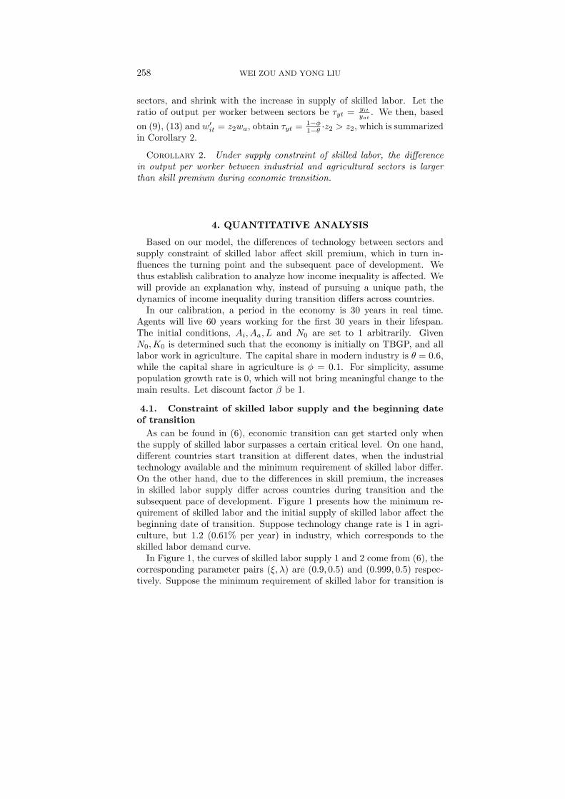
As can be found in (6), economic transition can get started only whenthe supply of skilled labor surpasses a certain critical level. On one hand,different countries start transition at different dates, when the industrialtechnology available and the minimum requirement of skilled labor differ.On the other hand, due to the differences in skill premium, the increasesin skilled labor supply differ across countries during transition and thesubsequent pace of development. Figure 1 presents how the minimum re-quirement of skilled labor and the initial supply of skilled labor affect thebeginning date of transition. Suppose technology change rate is 1 in agri-culture, but 1.2 (0.61% per year) in industry, which corresponds to theskilled labor demand curve.

In Figure 1, the curves of skilled labor supply 1 and 2 come from (6), thecorresponding parameter pairs (ξ, λ) are (0.9, 0.5) and (0.999, 0.5) respec-tively. Suppose the minimum requirement of skilled labor for transition is


!

FIG. 1. Initial skilled labor, minimum requirement of skilled labor and the beginningdate of transitionNote: Skilled labor demand corresponds to industrial technology change at rate of 1.2.The curves of “skill labor supply” 1 and 2 come from (6), with initial shares of skill laborof 0.1 and 0.001 respectively, the corresponding parameter pairs of (ξ, λ) are (0.9, 0.5)and (0.999, 0.5) respectively. The minimum requirement of skilled labor for transition is

defined by ξ = 0.8.

ξ = 0.8. The initial supply of skilled labor is very low (0.001) for “skilledlabor supply 2”, which leads to skilled labor shortage and higher skill pre-mium when the industrial technology is low. The supply of skilled labor isstimulated to increase faster at period 2 and reaches the minimum require-ment of skilled labor at around period 2.4. As for “skilled labor supply 1”,the initial share of skilled labor is higher (but not as high as 0.2, the mini-mum requirement for transition), and the supply of skilled labor moves toa quick increase around period 3, when the industrial technology is higher,and reaches the turning point of transition at around period 3.2.

Given technology change rate of 1.2, Figure 1 presents a situation thatthe economy with lower initial skilled labor may take off earlier than theeconomy with higher initial skilled labor. Why is the case? As Proposition1 and (21) show, the low initial skilled labor in an economy may delay itseconomic take-off (level effect), however, the supply of skilled labor maystart to increase faster at earlier data because the skill premium is higher(growth effect). If the growth effect dominates, the economy with lowerinitial skilled labor can take off earlier than an economy with higher initialskilled labor. Nevertheless, two implied prerequisites work: (1) there isminimum requirement of skilled labor for take-off; (2) the supply of skilledlabor should be elastic with respect to skill premium. Also in Figure 1,if the minimum requirement of skilled labor share is lower (say, 0.1), thenthe economy with higher initial skilled labor (skill labor supply 1) willtake off earlier (at period 1), while the economy with lower initial skilled


labor (skill labor supply 2) will wait at least 30 years to take off. Whetherskilled labor supply is sensitive to skill premium depends on many factors,including education system, culture, history, as well as technology growthrate.

!

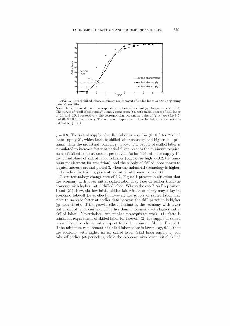
FIG. 2. Technology change, skill premium and economic take-offNote: Skilled labor demand corresponds to industrial technology change at rate of 1.3.The curves of “skill labor supply” 1, 2 and 3 come from (6), the corresponding parameterpairs of (ξ, λ) are (0.9, 0.9) and (0.999, 0.5) and (0.9, 0.5) respectively. The minimum

requirement of skilled labor for transition is defined by ξ = 0.8.

In Figure 2, skilled labor demand represents a higher rate of technol-ogy change (1.3 per period or 0.88% per year). “Skilled labor supply 2”corresponds to low initial level and high growth rate of skilled labor. Theinitial skilled labor is the same for “skilled labor supply 1” and “skilledlabor supply 3”, but the growth rate for the latter is much higher. Giventhis higher technology change, skill premium occurs earlier even for theeconomy with relatively higher initial skilled labor. The economy repre-sented by “skilled labor supply 3” enlarges its supply of skilled labor ataround period 2, and reaches the turning point of transition at around 2.4period (earlier than the economy represented by “skilled labor supply 2”).We thus conclude that higher technology change is a necessary conditionfor an economy with relative abundant skilled labor to take the lead ineconomic transition. Meanwhile, we find that an economy represented by“skilled labor supply 1” will not reach its turning point until around 3.2period, more than 30 years later than economy with “skilled labor sup-ply 3”, and about 20 years later than economy with “skilled labor supply2”. We again conclude that a prerequisite for an economy with relativelyabundant skilled labor to take off earlier is that its supply of skilled laborshould be sensitive to skill premium.


4.2. Skill premium, economic transition and the dynamics ofinequality

We now focus on how the constraint of skilled labor affects the dynamicsof inequality during transition. The technology of agriculture is set to1. We consider a higher technology change rate of 1.4 (1.13% annually)and a lower technology change rate of 1.2 (0.61% annually). In order toconcentrate on the pace of transition, we adjust the initial capital stock tomake sure that an economy without any constraint of skilled labor reachesturning point at the beginning of period 1. The supply of skilled labor isthus simplified as:

Qt = 1− ξλt (6′)

where λ(0 ≤ λ ≤ 1) is the change rate of unskilled labor, and initiallyQ0 = 1 − ξ. We consider three combinations of skilled labor supply atthe turning point. The curve “skilled labor supply 1” with parameters ofξ = 0.1and λ = 0.9 corresponds with the case of high initial level and lowgrowth rate of skilled labor. Curve “skilled labor supply 2” with parametersof ξ = 0.9 and λ = 0.5 corresponds with the case of low initial level andhigh growth rate of skilled labor. For the case of low initial level and lowgrowth rate of skilled labor, we set ξ = 0.9 and λ = 0.9 in “skilled laborsupply 3”.

In comparison with (6’), we consider a linear function of skilled laborsupply, and an arctan function of skilled labor supply. The latter meanswhen the amount of skilled labor is initially low, the increase in its supplyis slow; the increase in supply of skilled labor accelerates as the fractionof skilled labor increases and finally slows down again when the fraction ofskilled labor is high enough. The functions are set as follows:

Q(t) = −0.2 + 0.15 ∗ t (26)

Q(t) =13

arctan(2.5 ∗ t− 10) + 0.5 (27)

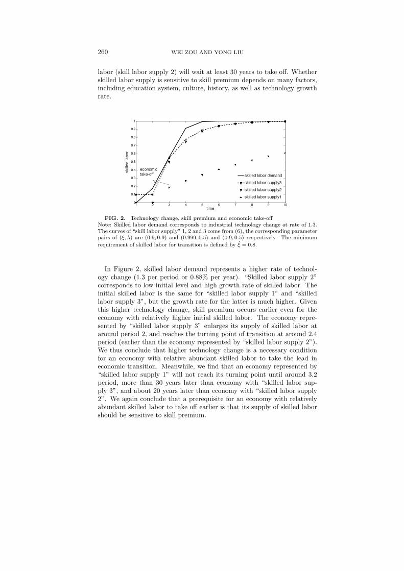
Figure 3 depicts the dynamic change of the demand for and supply ofskilled labor during economic transition. The demand curves and corre-spond to low and high growth rates of technology respectively. In Figure3(a), given low rate of technology change, the supply constraint of skilledlabor occurs the latest in “supply of skilled labor 1” (around period 3.5),but occurs earlier in “supply of skilled labor 2” (around period2.5), andeven earlier in “supply of skilled labor 3” (about period 0.3, or 10 yearsafter the turning point). The comparison between Figure 3 (c) and (a)shows that with higher rate of technology change in industrial sectors, thesupply constraint of skilled labor will not occur until later time given the


14

1 2 3 4 5 6 7 80

0.2

0.4

0.6

0.8

1

time

skill

ed la

bor

(a)

1 2 3 4 5 6 7 80

0.2

0.4

0.6

0.8

1

time

skill

ed la

bor

（b）

1 2 3 4 5 6 7 80

0.2

0.4

0.6

0.8

1

time

skill

ed la

bor

(c)

1 2 3 4 5 6 7 80

0.2

0.4

0.6

0.8

1

time

skill

ed la

bor

(d)

skilled labor demand blinear skilled labor supplyarg-tan skilled labor supply

skilled labor demand alinear skilled labor supplyarg-tan skilled labor supply

skilled labor demand bskilled labor supply1skilled labor supply2skilled labor supply3

skilled labor demand askilled labor supply1skilled labor supply2skilled labor supply3

Figure 3. Demand for and supply of skilled labor

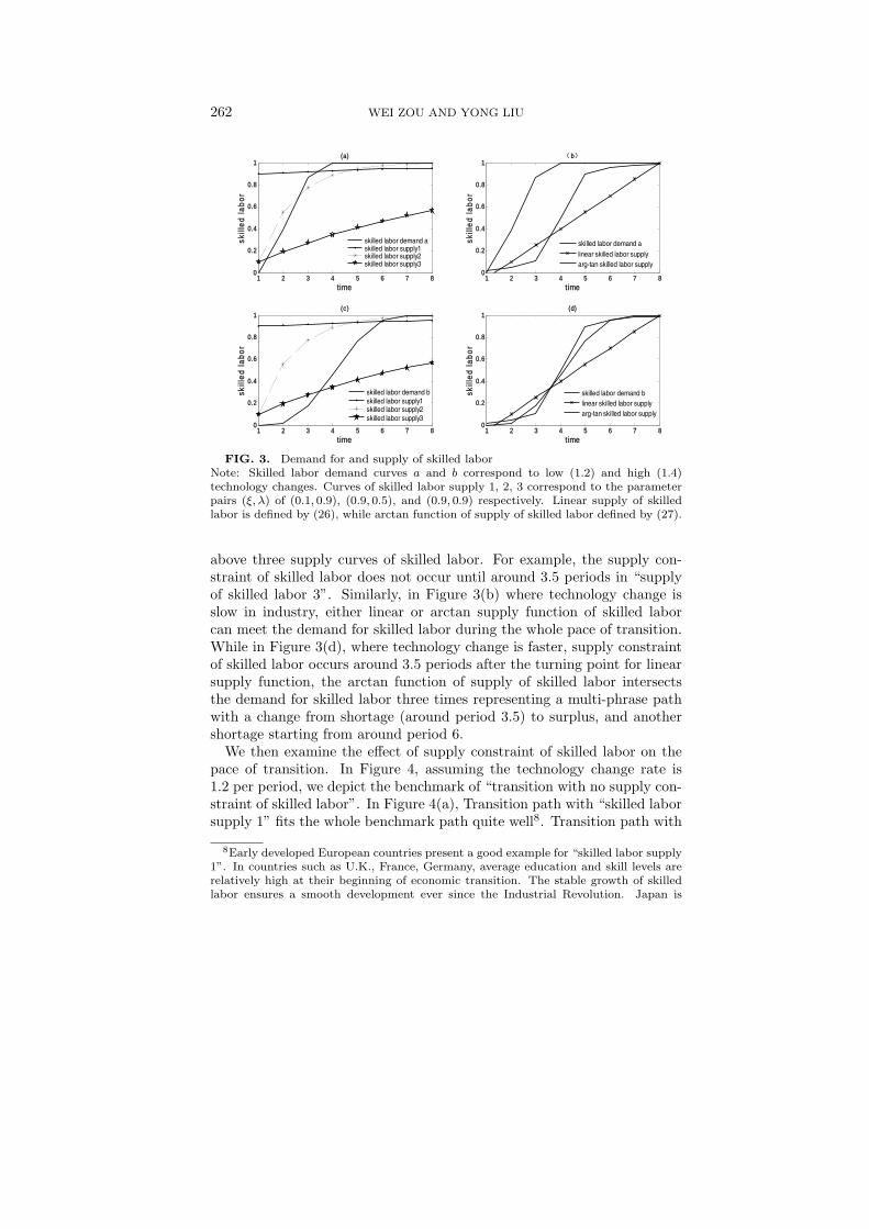
Note: Skilled labor demand curves a and b correspond to low (1.2) and high (1.4) technology changes. Curves of skilled labor supply 1, 2, 3 correspond to the parameter pairs ( ),ξ λ of (0.1, 0.9), (0.9,0.5), and (0.9, 0.9) respectively. Linear supply of skilled labor is defined by (26), while arctan function of supply of skilled labor defined by (27). Figure 3 depicts the dynamic change of the demand for and supply of skilled labor during economic transition. The demand curves a and b correspond to low and high growth rates of technology respectively. In Figure 3(a), given low rate of technology change, the supply constraint of skilled labor occurs the latest in “supply of skilled labor 1” (around period 3.5), but occurs earlier in “supply of skilled labor 2” (around period2.5), and even earlier in “supply of skilled labor 3” (about period 0.3, or 10 years after the turning point). The comparison between Figure 3 (c) and (a) shows that with higher rate of technology change in industrial sectors, the supply constraint of skilled labor will not occur until later time given the above three supply curves of skilled labor. For example, the supply constraint of skilled labor does not occur until around 3.5 periods in “supply of skilled labor 3”. Similarly, in Figure 3(b) where technology change is slow in industry, either linear or arctan supply function of skilled labor can meet the demand for skilled labor during the whole pace of transition. While in Figure 3(d), where technology change is faster, supply constraint of skilled labor occurs around 3.5 periods after the turning point for linear supply function, the arctan function of supply of skilled labor intersects the demand for skilled labor three times representing a multi-phrase path with a change from shortage (around period 3.5) to surplus, and another shortage starting from around period 6.

FIG. 3. Demand for and supply of skilled laborNote: Skilled labor demand curves a and b correspond to low (1.2) and high (1.4)technology changes. Curves of skilled labor supply 1, 2, 3 correspond to the parameterpairs (ξ, λ) of (0.1, 0.9), (0.9, 0.5), and (0.9, 0.9) respectively. Linear supply of skilledlabor is defined by (26), while arctan function of supply of skilled labor defined by (27).

above three supply curves of skilled labor. For example, the supply con-straint of skilled labor does not occur until around 3.5 periods in “supplyof skilled labor 3”. Similarly, in Figure 3(b) where technology change isslow in industry, either linear or arctan supply function of skilled laborcan meet the demand for skilled labor during the whole pace of transition.While in Figure 3(d), where technology change is faster, supply constraintof skilled labor occurs around 3.5 periods after the turning point for linearsupply function, the arctan function of supply of skilled labor intersectsthe demand for skilled labor three times representing a multi-phrase pathwith a change from shortage (around period 3.5) to surplus, and anothershortage starting from around period 6.

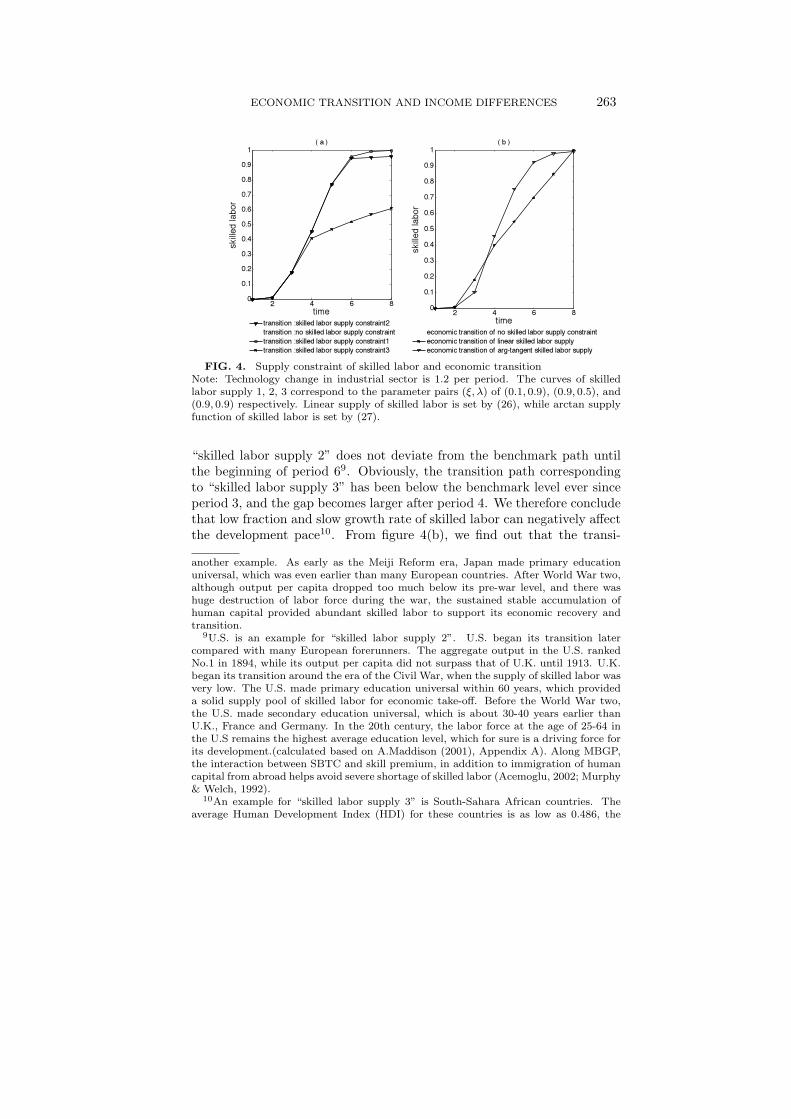
We then examine the effect of supply constraint of skilled labor on thepace of transition. In Figure 4, assuming the technology change rate is1.2 per period, we depict the benchmark of “transition with no supply con-straint of skilled labor”. In Figure 4(a), Transition path with “skilled laborsupply 1” fits the whole benchmark path quite well8. Transition path with

8Early developed European countries present a good example for “skilled labor supply1”. In countries such as U.K., France, Germany, average education and skill levels arerelatively high at their beginning of economic transition. The stable growth of skilledlabor ensures a smooth development ever since the Industrial Revolution. Japan is


!

FIG. 4. Supply constraint of skilled labor and economic transitionNote: Technology change in industrial sector is 1.2 per period. The curves of skilledlabor supply 1, 2, 3 correspond to the parameter pairs (ξ, λ) of (0.1, 0.9), (0.9, 0.5), and(0.9, 0.9) respectively. Linear supply of skilled labor is set by (26), while arctan supplyfunction of skilled labor is set by (27).

“skilled labor supply 2” does not deviate from the benchmark path untilthe beginning of period 69. Obviously, the transition path correspondingto “skilled labor supply 3” has been below the benchmark level ever sinceperiod 3, and the gap becomes larger after period 4. We therefore concludethat low fraction and slow growth rate of skilled labor can negatively affectthe development pace10. From figure 4(b), we find out that the transi-

another example. As early as the Meiji Reform era, Japan made primary educationuniversal, which was even earlier than many European countries. After World War two,although output per capita dropped too much below its pre-war level, and there washuge destruction of labor force during the war, the sustained stable accumulation ofhuman capital provided abundant skilled labor to support its economic recovery andtransition.

9U.S. is an example for “skilled labor supply 2”. U.S. began its transition latercompared with many European forerunners. The aggregate output in the U.S. rankedNo.1 in 1894, while its output per capita did not surpass that of U.K. until 1913. U.K.began its transition around the era of the Civil War, when the supply of skilled labor wasvery low. The U.S. made primary education universal within 60 years, which provideda solid supply pool of skilled labor for economic take-off. Before the World War two,the U.S. made secondary education universal, which is about 30-40 years earlier thanU.K., France and Germany. In the 20th century, the labor force at the age of 25-64 inthe U.S remains the highest average education level, which for sure is a driving force forits development.(calculated based on A.Maddison (2001), Appendix A). Along MBGP,the interaction between SBTC and skill premium, in addition to immigration of humancapital from abroad helps avoid severe shortage of skilled labor (Acemoglu, 2002; Murphy& Welch, 1992).

10An example for “skilled labor supply 3” is South-Sahara African countries. Theaverage Human Development Index (HDI) for these countries is as low as 0.486, the


tion pace corresponding with linear supply of skilled labor is located belowthe benchmark path ever since around period 3.5, and the gap reachesits summit around period 6. Corresponding to arctan supply function ofskilled labor, the transition path is below benchmark from period 2 to3.5, and then it fits the benchmark locus well, it finally turns to be lowerthan benchmark level since the beginning of period 5 because the supplyof skilled labor becomes growing slower.

16

figure 4(b), we find out that the transition pace corresponding with linear supply of skilled labor is located below the benchmark path ever since around period 3.5, and the gap reaches its summit around period 6. Corresponding to arctan supply function of skilled labor, the transition path is below benchmark from period 2 to 3.5, and then it fits the benchmark locus well, it finally turns to be lower than benchmark level since the beginning of period 5 because the supply of skilled labor becomes growing slower.

1 2 3 4 5 6 7 80

2

4

6

8

10

time

wag

e ra

tio

（a）

1 2 3 4 5 6 7 80

0.5

1

1.5

2

2.5

3

3.5

time

wag

e ra

tio

(b)

1 2 3 4 5 6 7 80

2

4

6

8

10

time

per

labo

r pr

oduc

t rat

io

(c)

1 2 3 4 5 6 7 80

2

4

6

8

time

per

labo

r pr

oduc

t rat

io

(d)

inequality path2inequality path1inequality path3

inequality path2inequality path1inequality path3

inequality path4inequality path5

inequality path4inequality path5

Figure 5. The dynamics of skill premium and differences in output per worker

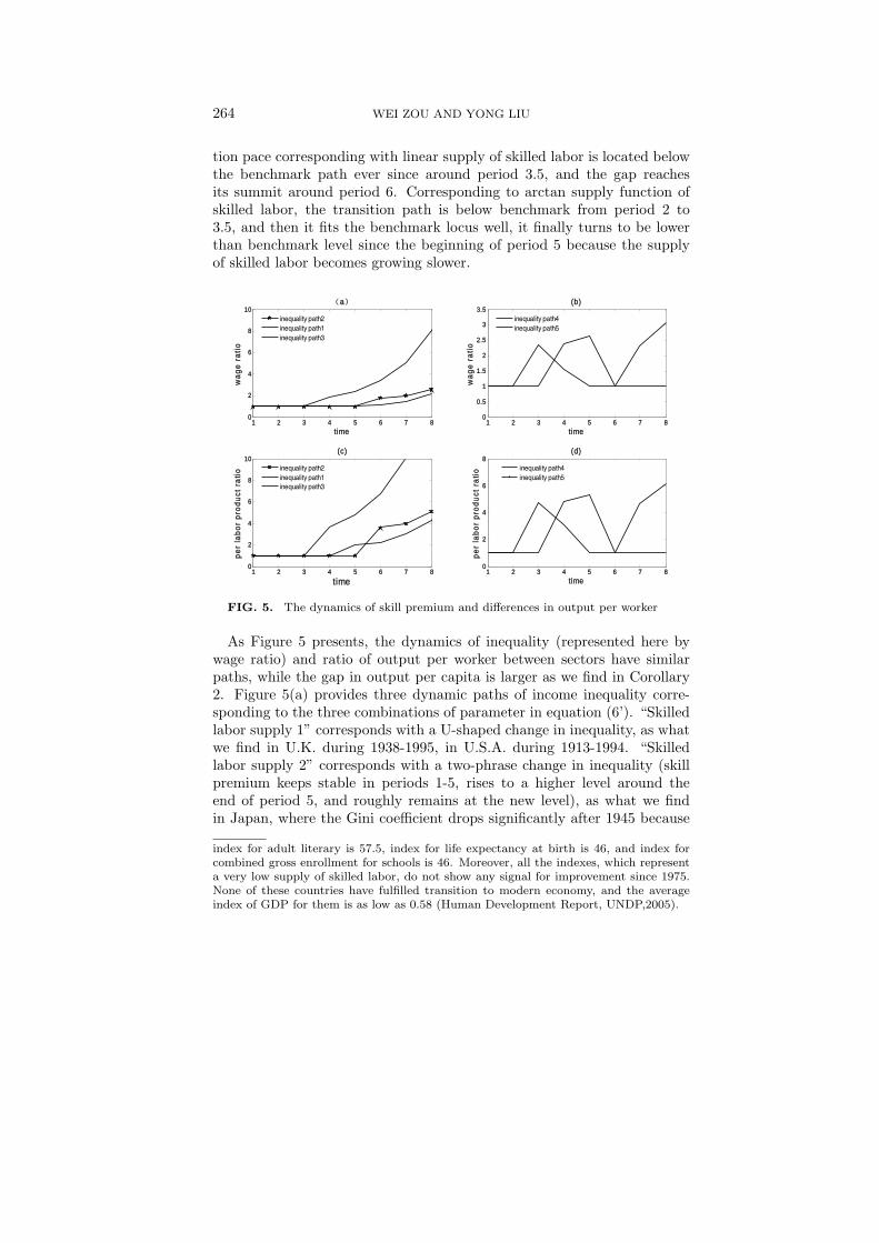
As Figure 5 presents, the dynamics of inequality (represented here by wage ratio) and ratio of output per worker between sectors have similar paths, while the gap in output per capita is larger as we find in Corollary 2. Figure 5(a) provides three dynamic paths of income inequality corresponding to the three combinations of parameter in equation (6’). “Skilled labor supply 1” corresponds with a U-shaped change in inequality, as what we find in U.K. during 1938-1995, in U.S.A. during 1913-1994. “Skilled labor supply 2” corresponds with a two-phrase change in inequality (skill premium keeps stable in periods 1-5, rises to a higher level around the end of period 5, and roughly remains at the new level), as what we find in Japan, where the Gini coefficient drops significantly after 1945 because of the relative abundant human capital and extreme shortage of physical capital then. “Skilled labor supply 3” corresponds with an upward sloping and steep curve in inequality, which shows that the low initial level and low growth of supply of skilled labor lead to large and accelerating enlarging inequality overtime. In Figure 5(b), the inequality path corresponding with linear supply of skilled labor turns out to be inverted U-shaped. Inequality increases significantly around period 3, and reaches its summit around period 5, and move into downward section until skill premium disappears along MBGP. The inequality in U.K. from 1688 to around 1900 is a typical example. As for the arctan supply function of skilled labor, the skilled labor is initially limited and growing slowly, which constrains transition from the very beginning period and make skill premium increasing. In the middle of transition, the increased supply of skilled labor surpasses the demand for it, and transition moves

FIG. 5. The dynamics of skill premium and differences in output per worker

As Figure 5 presents, the dynamics of inequality (represented here bywage ratio) and ratio of output per worker between sectors have similarpaths, while the gap in output per capita is larger as we find in Corollary2. Figure 5(a) provides three dynamic paths of income inequality corre-sponding to the three combinations of parameter in equation (6’). “Skilledlabor supply 1” corresponds with a U-shaped change in inequality, as whatwe find in U.K. during 1938-1995, in U.S.A. during 1913-1994. “Skilledlabor supply 2” corresponds with a two-phrase change in inequality (skillpremium keeps stable in periods 1-5, rises to a higher level around theend of period 5, and roughly remains at the new level), as what we findin Japan, where the Gini coefficient drops significantly after 1945 because

index for adult literary is 57.5, index for life expectancy at birth is 46, and index forcombined gross enrollment for schools is 46. Moreover, all the indexes, which representa very low supply of skilled labor, do not show any signal for improvement since 1975.None of these countries have fulfilled transition to modern economy, and the averageindex of GDP for them is as low as 0.58 (Human Development Report, UNDP,2005).


of the relative abundant human capital and extreme shortage of physicalcapital then. “Skilled labor supply 3” corresponds with an upward slopingand steep curve in inequality, which shows that the low initial level and lowgrowth of supply of skilled labor lead to large and accelerating enlarginginequality overtime.

In Figure 5(b), the inequality path corresponding with linear supply ofskilled labor turns out to be inverted U-shaped. Inequality increases signif-icantly around period 3, and reaches its summit around period 5, and moveinto downward section until skill premium disappears along MBGP. The in-equality in U.K. from 1688 to around 1900 is a typical example. As for thearctan supply function of skilled labor, the skilled labor is initially limitedand growing slowly, which constrains transition from the very beginningperiod and make skill premium increasing. In the middle of transition, theincreased supply of skilled labor surpasses the demand for it, and transitionmoves closer to the benchmark pace (see Figure 4(b)), which shrinks skillpremium. In the later period of transition, supply of skilled labor decreasesagain, which leads to increasing inequality after the beginning of period 6.It thus corresponds with an N-shaped change of inequality as what we findin U.K. during 1688-1995.

5. CONCLUSIONS

Based on Hansen & Prescott (2002), we introduce skill differences inlabor, and construct a dynamic model of economic transition. The modelsof Hansen & Prescott (2002) and Ngai (2004) make the assumption of laborindifferences so that any labor can get involved in agricultural or industrialproduction. We assume there is significant difference in labor skills, eitherunskilled or skilled labor can be employed in agriculture, while only skilledlabor can match modern technology in industrial sectors. Therefore, due tothe differences in the initial stock of skilled labor and its growth rate, theturning point of transition may be delayed, and the path of transition maybe affected. The supply constraint affects both the beginning date and thesubsequent pace of modern growth, and thus in turn affects the dynamicsof income distribution.

We provide another approach to the mechanism of economic transitionand long-run growth. Romer (1986) establishes an increasing-return modeland explains the long-run non-deceasing growth in most European indus-trial countries. Other researchers explain the cross-country differences intransition and growth with externalities (Lucas, 1988), barriers to invest-ment (Ngai, 2004), or economy of scale (Wang & Xie, 2003). In our model,the production functions of both agriculture and industry exhibit constantreturn to scale. We prove that, without any consideration of externalitiesor barriers to private investment, the differences in labor skills and in tech-


nologies across sectors make it possible for skilled labor to transform intomodern industry. There will thus be continuous capital deepening in indus-try, which in turn results in continuous growth in output per capita. OnMBGP, all labor is skilled labor, and the economy is growing at a constantrate.

Our simulation and quantitative analysis present more evidences whycross-country output per capita and income distribution are so different.To a great extent, the differences in technologies cross sectors and in theinitial stock of skilled labor explain the dynamics of income distributionovertime. If the initial stock of skilled labor is low, and growing at alow rate, then there will be huge delay in the beginning date of economictransition, and income inequality will be increasing over a longer period.Given technology progress, the supply constraint and the dynamic changeof skilled labor result in multiple possible paths of income distribution,such as “U-shaped”, “inverted-U-shaped” or “N-shaped” ones.

We also argue that the income inequality during economic transition ishigher than that on balanced growth paths, which means a substantialfraction of existing income differences is transitional. Therefore, duringeconomic transition, not only faster technology progress, but also moreinvestment on education and skill formation are recommended to reducethe supply constraint of skilled labor, facilitate economic transition andlong-run growth, and decrease income inequality.

APPENDIX AThe dynamics of inequality and transition in U.K., U.S.A. andJapan

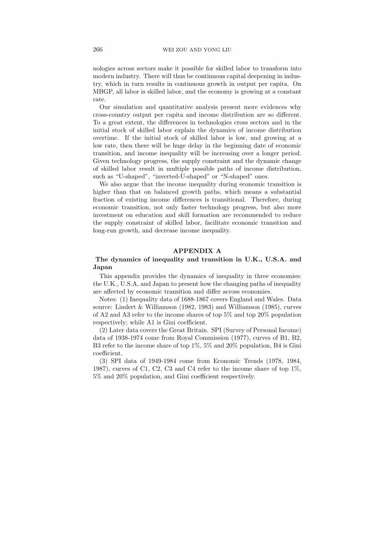
This appendix provides the dynamics of inequality in three economies:the U.K., U.S.A, and Japan to present how the changing paths of inequalityare affected by economic transition and differ across economies.

Notes: (1) Inequality data of 1688-1867 covers England and Wales. Datasource: Lindert & Williamson (1982, 1983) and Williamson (1985), curvesof A2 and A3 refer to the income shares of top 5% and top 20% populationrespectively; while A1 is Gini coefficient.

(2) Later data covers the Great Britain. SPI (Survey of Personal Income)data of 1938-1974 come from Royal Commission (1977), curves of B1, B2,B3 refer to the income share of top 1%, 5% and 20% population, B4 is Ginicoefficient.

(3) SPI data of 1949-1984 come from Economic Trends (1978, 1984,1987), curves of C1, C2, C3 and C4 refer to the income share of top 1%,5% and 20% population, and Gini coefficient respectively.


!

FIG. A.1 Evolution of income inequality in UK:1688-1995

(4) Data of 1977-1995 come from Economic Trends (1994, 1995, 1997),and curves of D1, D2 refer to income share of top 20% population and Ginicoefficient respectively.

!

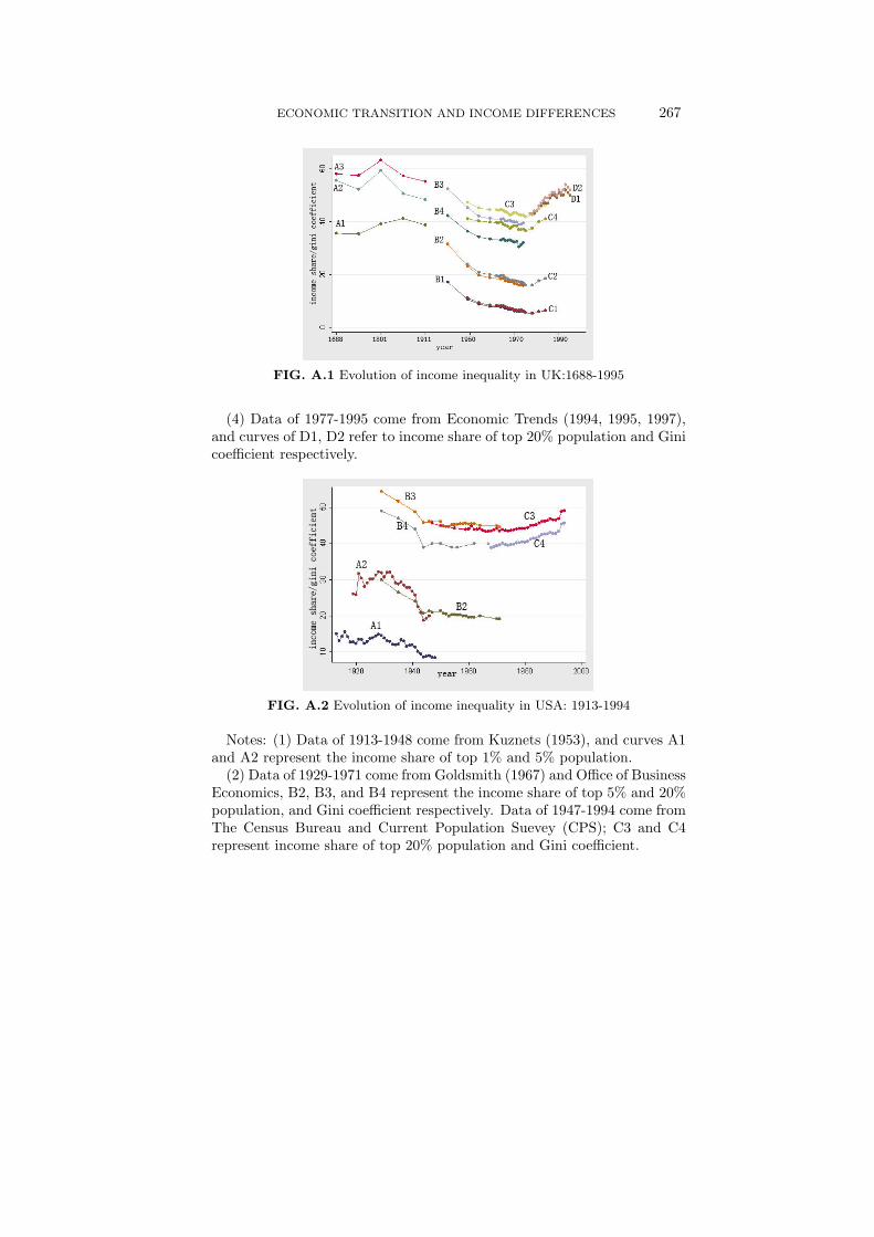
FIG. A.2 Evolution of income inequality in USA: 1913-1994

Notes: (1) Data of 1913-1948 come from Kuznets (1953), and curves A1and A2 represent the income share of top 1% and 5% population.

(2) Data of 1929-1971 come from Goldsmith (1967) and Office of BusinessEconomics, B2, B3, and B4 represent the income share of top 5% and 20%population, and Gini coefficient respectively. Data of 1947-1994 come fromThe Census Bureau and Current Population Suevey (CPS); C3 and C4represent income share of top 20% population and Gini coefficient.


!

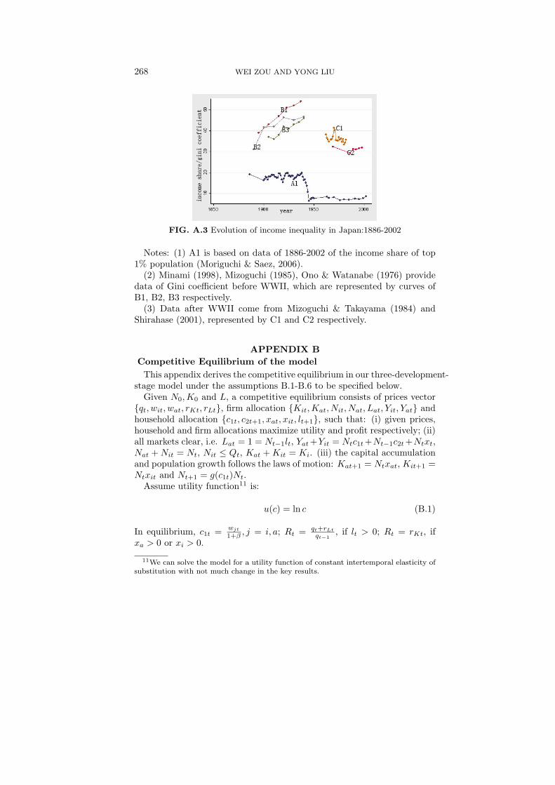
FIG. A.3 Evolution of income inequality in Japan:1886-2002

Notes: (1) A1 is based on data of 1886-2002 of the income share of top1% population (Moriguchi & Saez, 2006).

(2) Minami (1998), Mizoguchi (1985), Ono & Watanabe (1976) providedata of Gini coefficient before WWII, which are represented by curves ofB1, B2, B3 respectively.

(3) Data after WWII come from Mizoguchi & Takayama (1984) andShirahase (2001), represented by C1 and C2 respectively.

APPENDIX BCompetitive Equilibrium of the model

This appendix derives the competitive equilibrium in our three-development-stage model under the assumptions B.1-B.6 to be specified below.

Given N0,K0 and L, a competitive equilibrium consists of prices vector{qt, wit, wat, rKt, rLt}, firm allocation {Kit,Kat, Nit, Nat, Lat, Yit, Yat} andhousehold allocation {c1t, c2t+1, xat, xit, lt+1}, such that: (i) given prices,household and firm allocations maximize utility and profit respectively; (ii)all markets clear, i.e. Lat = 1 = Nt−1lt, Yat +Yit = Ntc1t +Nt−1c2t +Ntxt,Nat + Nit = Nt, Nit ≤ Qt, Kat + Kit = Ki. (iii) the capital accumulationand population growth follows the laws of motion: Kat+1 = Ntxat, Kit+1 =Ntxit and Nt+1 = g(c1t)Nt.

Assume utility function11 is:

u(c) = ln c (B.1)

In equilibrium, c1t = wjt

1+β , j = i, a; Rt = qt+rLt

qt−1, if lt > 0; Rt = rKt, if

xa > 0 or xi > 0.

11We can solve the model for a utility function of constant intertemporal elasticity ofsubstitution with not much change in the key results.


B.1. TRADITIONAL BALANCED GROWTH PATH (TBGP)

On TBGP, all workers work in traditional agriculture. The function ofpopulation growth g(·) is chosen so that both output per capita (or perworker) (ya) and capital per capita (ka) are constant. Assume:

g(c1a) = γ1/(1−µ−φ)a , and g(c1) > g(c1a), ∀c1 ∈ [c1a, c1a+ε], ε > 0 (B.2)

then output per capita will be constant: ya = Aaγtakφ

aNµ+φ−1t . Define

capital-output ratio on TBGP as νa = ka/ya, where

νa =(1 + β − µ)−

√(1 + β − µ)2 − 4µφβ(1 + β)

2(1 + β)γ1/(1−µ−φ)a

. We thus have ya =

[Aaγtaνφ

a Nµ+φ−1t ]1/(1−φ).

On TBGP, The price and rental rate of land grow at γ1/(1−µ−φ)a , while

the wage rate and rental rate of capital are constant.

B.2. TRANSITIONB.2.1. The case when the supply of skilled labor is abundant

(Nit ≤ Qt)When a firm starts to use modern technology, its optimization problem

is:

Ψ(rKt, wit) = maxKit,Na

(AiγtiK

θitN

1−θit − rKtKit − witNit)

The optimal decision of the firm implies: Kit

Nit= θwit

(1−θ)rKt, so the profit

function becomes:

Ψ(rKt, wit) = maxNit

[Aiγ

ti

(θwit

(1− θ)rKt

)θ

− wit

1− θ

]Nit

Because only skilled labor can match the modern technology used in in-dustry, the workers that can be transformed to industry are skilled labor,who can earn “skill premium” in industrial sector. The wage rates in agri-culture and industry are thus different. Assume wit = z1wat, where z1 > 1is the skill premium under the condition of Nit < Qt. Therefore, the profitfunction can be written as:

Ψ(rKt, wat) = maxNa

[Aiγ

ti

(θz1wat

(1− θ)rKt

)θ

− z1wat

1− θ

]Nit


Along TBGP, the firm will use modern technology if Ψ(rK , wa) ≥ 0. Thecondition of transform to modern industry is:


1

(wa

1− θ

)1−θ (rK

θ

)θ

B.2.2. The case when the supply of skilled labor is constrained(Nit > Qt)

In this case, the optimization problem a firm faces when it starts to usemodern technology is:

Ψ(rKt, w′a) = max

Ka,Na

(AiγtiK

θitQ

1−θt − rKtKit − w′

itQt)

The optimal decision of the firm requires: Kit

Qt= θw′

a

(1−θ)rKt, and the profit

function becomes:

Ψ(rKt, w′it) = max

Qt

[Aiγ

ti

(θw′

it

(1− θ)rKt

)θ

− w′it

1− θ

]Qt

Due to the scarcity of skilled labor, industrial sector will provide a wagerate of w′

it = z2wat, where z2 is skill premium when the supply of skilledlabor is constrained. Because industry has to pay more to attract skilledlabor, the skill premium in this case is higher than that in the case withabundant supply of skilled labor, i.e. z2 > z1. The profit function is thusrewritten as:

Ψ(rKt, wat) = maxQt

[Aiγ

ti

(θz2wat

(1− θ)rKt

)θ

− z2wat

1− θ

]Qt

Again, along TBGP, the firm will use modern technology if Ψ(rK , wa) ≥ 0,and the condition of transform to modern industry is:

Ait = Aiγti ≤ z1−θ

2

(wa

1− θ

)1−θ (rK

θ

)θ

.

Obviously, because z2 > z1, the supply constraint of skilled labor makesit even more difficult for the condition of transform to be satisfied, theeconomic transition is therefore expected to delay. However, the higher skillpremium can provide more incentive for skill formation, and the supply ofskilled labor will increase until it can satisfy the demand for skill labor inindustry. Our following discussion on transition will focus on the case ofNit ≤ Qt.


B.2.3. The path of transitionGiven the initial condition K0 = (Nµ

0 νa)1/(1−φ), rK and wa can be rep-resented as function of N0. The turning point of economic transition t∗

satisfies:

Aiγt∗

i ≥ Bz1−θ1

(1

N0

)(1−µ−φ)(1−θ)/(1−φ)

> Aiγt∗−1i

where B =(

φθ

)θ (µ

1−θ

)1−θ

(ν(φ−θ)a A

(1−θ)a )1/(1−φ).

Given qt−1, Nt and land normalized to 1 (L = 1), the total value ofinvestment of younger generation in period (t − 1) is: It = Nt−1(wjt−1 −c1t−1)− qt−1, j = i, a. Profit maximization implies:

θYit

Kit=

φYat

Kat, wit = (1− θ)

Yit

Nit, wat = µ

Yat

Nat, rLt = (1− φ− µ)Yat

Taking into account wit = z1wat, and assuming:

θ > φ (B.3)

we have: kat = ϕz1

kit, where kat = Kat/Nat, kit = Kit/Nit, and ϕ =(1−θ)φ

θµ < 1.

Market clearing requires: kat = (ϕ/z1)·(It/Nt)(1−(1−ϕ/z1)nat)

, where nat = Nat/Nt.Because there are skill differences in labor, while the returns of capital areequal across sectors, we have:

kθ−φat =

φ

θ

Aat

Ait

(ϕ

z1

)θ−1

Nµ+φ−1at .

Therefore, the equilibrium n∗at solves f(n∗at) = 0, where

f(nat) =φ

θ

(ϕ

z1

)φ−1

(1− (1− ϕ/z1)nat)θ−φ − Ait

AatIθ−φt N1−θ−µ

t n1−φ−µat

where 1 − µ − φ > 0 and t ≥ t∗ implies f ′ < 0, f(0) > 0, and f(1) < 0.Thus there exists a unique n∗at ∈ [0, 1).

We further assume:

γi > γa (B.4)

∃t, n, s.t. g(cit) ≤ n ∀t > t if 1− θ < µ (B.5)

g(c1t) ≥ 1 if 1− θ ≥ µ


then Ait

AatIθ−φt N1−µ−θ

t is an increasing function of time t, and n∗at convergesto zero. Since the share of labor working in agriculture will converge to 0,the share of skilled labor in total labor will increase overtime i.e. in thelimit, Qt → Nt.

Meanwhile, the skill premium z1 plays a role in the above function off(nat) where it makes the first term smaller and the second term larger(through increasing It), so it helps to make the transition faster. If thereis supply constrain of skilled labor in the economy, the skill premium (z2)will be higher, which may make the above mechanism more significant.

B.3. MODERN BALANCED GROWTH PATH (MBGP)

As the economy transforms to modern economy, n∗at converges to 0, bothrLt → 0 and qt → 0. Assume:

limc1→∞

g(c1) = g (B.6)

the economy converges to MBGP. Output per capita (yit) is growing ata constant rate. The capital-output ratio of modern economy is νi =

β(1−θ)

(1+β)γ1/(1−θ)i

, and output per capita thus equals to: yit = (Aiγtiν

θi )1/(1−θ).

All labor are skilled labor, and the wage and consumption grow at a rateof γ

1/(1−θ)i .

REFERENCESAcemoglu, D., 2002. Directed Technical Change. The Review of Economic Studies69, 781-809

Acemoglu, D., 2000. Technical Change, Inequality, and the Labor Market. Mimeo,MIT.

Acemoglu, D., 1998. Why Do New Technologies Complement Skill? Directed Techni-cal Change and Wage Inequality. Quarterly Journal of Economics 113, 1055-1090.

Acemoglu, D., 2003. Patterns of Skill Premia. Review of Economic Studies (70),199-230.

Aghion, P., 2002. Schumpeterian Growth Theory and the Dynamics of Income In-equality. Econometrica 70, 855-882.

Aghion, P, E. Caroli, and C. Garcia-Perialosa, 1999. Inequality and Economic Growth:The Perspective of the New Growth Theories. Journal of Economic Literature 37,1615-1660.

Aghion, P. and P. Bolton, 1997. A Trickle-down Theory of Growth and Developmentwith Debt Overhang. Review of Economic Studies 64, 151-72.

Aghion and Howitt, 1992. A Model of Growth Through Creative Destruction. Econo-metrica 60, 323-351.

Alesina and Rodrik, 1994. Distributive Politics and Economic Growth. QuarterlyJournal of Economics 109, 465-490.


Ahluwalia, M. S., 1976. Income Distribution and Development: Some Stylized Facts.American Economic Review, Papers and Proceedings 66, 128-135.

Ahluwalia, M. S., 1976. Inequality, Poverty and Development. Journal of DevelopmentEconomics 3, 307-342.

Aitken, Brian, Ann Harrison, Robert E. Lipsey, 1996. Wages and Foreign Owner-ship: A Comparative Study of Mexico, Venezuela, and the United States. Journal ofInternational Economics 40, 345-371.

Anand, S. and R. Kanbur, 1993. The Kuznets Process and the Inequality DevelopmentRelationship. Journal of Development Economics 40, 25-52

Anand, S. and R. Kanbur, 1993. Inequality and Development: A Critique. Journal ofDevelopment Economics 41, 19-43.

Barro, R. J. 2000. Inequality and growth in a panel of countries. Journal of EconomicGrowth Vol. 5, No 1, 87-120.

Barro, J. R., and X. Sala-i-Martin, 2002.Economic Growth. Second Edition, Cam-bridge: The MIT Press.

Benabou, R., 1996. Heterogeneity, Stratification, and Growth: Macroeconomic Impli-cations of the Community Structure and Social Finance. American Economic Review86, 584-609.

Benabou, R., 1996. Equity and Efficiency in Human Capital Investment: The LocalConnection. Review of Economic Studies 63, 237-264.

Berman, E., J. Bound and Z. Griliches, 1994. Changes in Demand for Skilled La-bor Within US Manufacturing: Evidence from the Annual Survey of Manufactures.Quarterly Journal of Economics 109:2, 367-97.

Deininger, K. and L. Squire, 1996. Measuring Income Inequality: A New Data Base.The World Bank Economic Review 10, 565-591.

Diamond, P.A., 1965. National Debt in a Neoclassical Growth Model. American Eco-nomic Review 55, 1126-1150.

Fields, G. and G. Jakubson, 1994. New Evidence on the Kuznets Curve. Mimeo(Cornell University, Ithaca).

Forbes, K., 2000. A Reassessment of the Relationship between Inequality and Growth.American Economic Review 90, 869-887.

Francois, J.F., and H. Rojas-Romagosa, 2008. Reassessing the Relationship betweenInequality and Development. CPB discussing paper, NO. 107.

Galor, O. and O. Moav, 2002. From Physical to Human Capital Accumulation: In-equality in the Process of Development. Brown University Working Paper No.99-27.

Galor, O. and D. Tisddon, 1997. Technological Progress, Mobility, and EconomicGrowth. American Economic Review 76, 363-382.

Galor O. and J. Zeira, 2003. Income Distribution and Macroeconomics. Review ofEconomic Studies 60, 35-52.

Garcia-Penalosa, C. and S. J. Turnovsky, 2004. Growth, Inequality, and Fiscal Policywith Endogenous Labor Supply: What are the Relevant Tradeoffs? Mimeo, Universityof Washington.

Goldsmith, S., 1967. Changes in the Size Distribution of Income, in E.C. Budd, (ed.),Inequality and Poverty (Harper and Row, New York), with an update in Budd’sintroduction.


Gylfason, T and G. Zoega, 2003. Inequality and Growth: Do Natural Resources Mat-ter? in Inequality and Growth: Theory and Policy Implications. T. S. Eicher and S.J. Turnovsky (eds.) Cambridge MA: MIT Press.

Hansen, G. D., and E. C. Prescott, 2002. Malthus to Solow. American EconomicReview 92, 1200-1217.

Hertal, T. and F. Zhai, 2006. Labor Market Distortions, Rural-Urban Inequality andthe Opening of China’s Economy. Economic Modeling 23, 76-109.

Kanbur, R., 2000. Income Distribution and Development. Handbook of Income Dis-tribution Volume 1, 791-841.

Kanbur, R. and X. Zhang, 2005. Fifty Years of Regional Inequality in China: AJourney Through Central Planning, Reform and Openness. Review of DevelopmentEconomics 9, 87-106.

Kuznets, S., 1955. Economic Growth and Inequality. American Economic Review 45,1-28.

Kuznets, S., 1953. Shares of Upper Income Groups in Income and Savings. New York:Columbia University Press.

Li, H. Y. and H. F. Zou, 1998. Income Inequality is not Harmful to Growth: Theoryand Evidence. Review of Development Economics 2, 318-334.

Lindert, P.H., 2000. Three Centuries of Inequality in Britain and American. In Atkin-son and Bourguignon (eds.) Handbook of Income Distribution Volume 1.

Lindert, P. H. and J. G. Williamson, 1982. Revising England’s Social Tables, 1688-1812.Explorations in Economic History 19, 385-408.

Lindert, P. H. and J. G. Williamson, 1983. Reinterpreting Britain’s SocialTables,1688-1813. Explorations in Economic History 20, 94-109.

Lucas, R., 1988. On the Mechanics of Economic Development. Journal of MonetaryEconomics 22(1), 3-42.

Lundberg, M. and L. Squire, 2003. The Simultaneous Evolution of Growth and In-equality. Economic Journal 113, 326-344.

Maddison, A., 2001. The World Economy: A Millennial Perspective, OECD.

Minami, R., 1998. Economic Development and Income Distribution in Japan: AnAssessment of the Kuznets Hypothesis. Cambridge Journal of Economics 22(1), 39-58.

Mizoguchi, T., 1985. Economic Development Policy and Income Distribution: theExperience in East and Southeast Asia. Journal of the Developing Economies 23(4),307-324.

Mizoguchi, T. and Takayama, N., 1984. Equity and Poverty under Rapid Economicgrowth: the Japanese Experience. Tokyo: Kinokuniya.

Moriguchi, C. and Saez, E., 2006. The Evolution of Income Concentration in Japan,1886-2002: Evidence From Income Tax Statistics. NBER Working papar No.12558.

Murphy, K. and F. Welch, 1992. The Structure of Wages. Quarterly Journal of Eco-nomics 107, 255-285.

Ngai, L.R., 2004. Barriers and the Transition to Modern Growth. Journal of MonetaryEconomics, 1353-1383

Persson, T. and G. Tabellini, 1994. Is Inequality Harmful for Growth? AmericanEconomic Review 84, 600-621.


Perotti, R., 1996. Growth, Income Distribution, and Democracy: What the Data Say.Journal of Economic Growth 1, 149-187.

Romer, P.M., 1986. Increasing Returns and Long-run Growth. Journal of PoliticalEconomy 94, 1002-37.

Saint-Paul, G. and T. Verdier, 1993. Education, Democracy, and Growth. Journal ofDevelopment Economics 42, 399-407.

Royal Commission on the Distribution of Income and Wealth, 1977. Report No.5,Third Report of the Standing Reference (HMSO , London).

Shirahase, S., 2001. Japanese Income Inequality by Household Types in ComparativePerspective. LIS working Paper No.268.

Sicular, T., X. Yue, B. Gustafsson and S. Li, 2007. The Urban-Rural Income Gapand Inequality in China. Review of Income and Wealth 53, 93-126.

Violante, G., 2002. Technological Acceleration, Skill Transferability and the Rise inResidual Inequality. Quarterly Journal of Economics 117(1), 297-338.

Wang, P. and D. Xie, 2003. Activation of a Modern Industry. Journal of DevelopmentEconomics, 393-410.

Williamson, J.G., 1985. Did British Capitalism Breed Inequality? Boston: Allen andUnwin.

Zhao, Y., 1999. Leaving the Countryside: Rural-to-Urban Migration Decisions inChina. American Economic Review 89, 281-286.

Skilled Labor, Economic Transition and Income Diﬀerences...

Documents

Transcript of Skilled Labor, Economic Transition and Income Diﬀerences...