Lecture 3 A Brief Review of Some Important Statistical Concepts.
MSDL presentation
A Brief Introduction to Statistical Mechanics
Indrani A. Vasudeva Murthy
Modelling, Simulation and Design Lab (MSDL)
School of Computer Science, McGill University, Montreal, Canada
13 May 2005. A Brief Introduction to Statistical Mechanics 1/36
Overview
• The Hamiltonian, the Hamiltonian equations of motion; simple
harmonic oscillator.
• Thermodynamics; internal energy and free energy.
• Kinetic theory; phase space and distribution functions.
• Statistical mechanics: ensembles, canonical partition function; the
ideal gas.
• Concluding remarks.
13 May 2005. A Brief Introduction to Statistical Mechanics 2/36

Equations of Motion
• Newton’s second law: F = ma.
• Equations of motion: explicit expressions for F, a.
• Different formulations give a recipe to arrive at this:
Lagrangian and Hamiltonian approaches.
• In Classical Mechanics, the Lagrangian formulation is most common –
leading to Lagrange’s equations of motion.
• The Hamiltonian formulation leads to Hamilton’s equations of motion.
• In Statistical Mechanics and Quantum Mechanics it is more
convenient to use the Hamiltonian formalism.
13 May 2005. A Brief Introduction to Statistical Mechanics 3/36

The Hamiltonian
• The Hamiltonian H is defined as follows:
H = T +V.
T : kinetic energy of the system,
V : potential energy of the system.
• For most systems, H is just the total energy E of the system.
• Knowing H , we can write down the equations of motion.
• In Classical Physics, H ≡ E , a scalar quantity.
• In Quantum Mechanics, H is an operator.
13 May 2005. A Brief Introduction to Statistical Mechanics 4/36

Generalized Coordinates• The concept of a ‘coordinate’ is extended, appropriate variables can
be used. For each generalized coordinate, there is a correspondinggeneralized momentum (canonically conjugate). Notation:
qi : generalized coordinates;
pi : generalized momenta.
• For example,{qi} ≡ Cartesian coordinates {x,y,z} for a free particle.{qi} ≡ the angle θ for a simple pendulum.
• Can transform between the regular coordinates and the generalizedcoordinates.
• Useful in dealing with constraints.
13 May 2005. A Brief Introduction to Statistical Mechanics 5/36

Generalized Coordinates
• Hamiltonian H = H ({qi},{pi}, t) = H (q, p, t).
• The generalized coordinates and momenta need not correspond to
the usual spatial coordinates and momenta.
• In general for N particles, we have 3N coordinates and 3N momenta.
• Coordinates and momenta are considered ‘conjugate’ quantities -
they are on an equal footing in the Hamiltonian formalism.
• Coordinates and momenta together define a phase space for the
system.
13 May 2005. A Brief Introduction to Statistical Mechanics 6/36
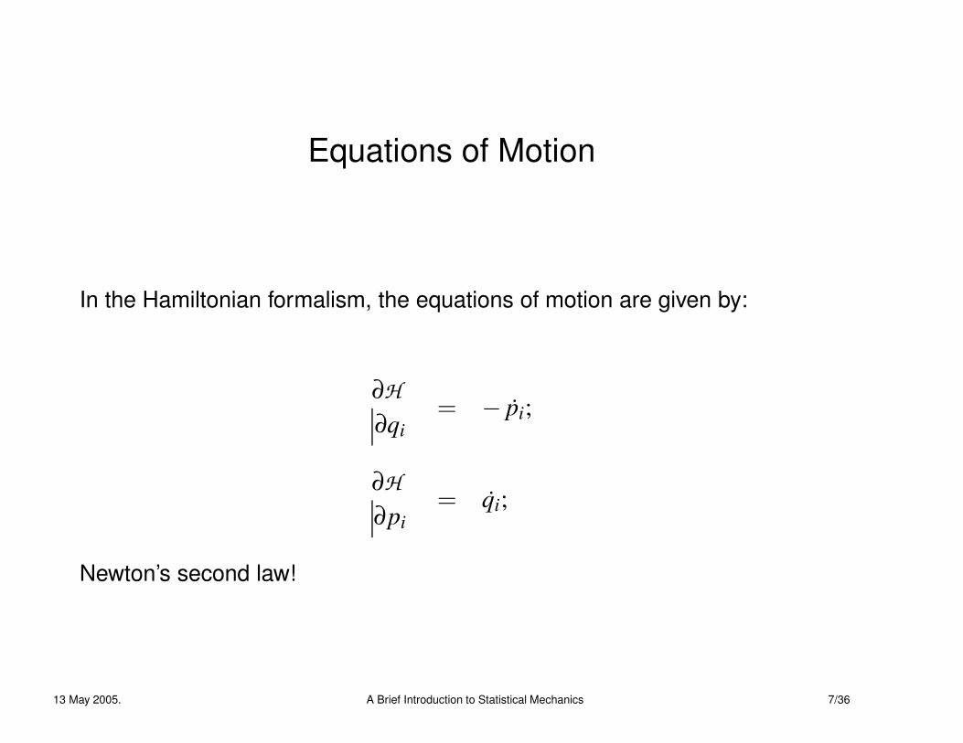
Equations of Motion
In the Hamiltonian formalism, the equations of motion are given by:
∂H∂qi
= − pi;
∂H∂pi
= qi;
Newton’s second law!
13 May 2005. A Brief Introduction to Statistical Mechanics 7/36
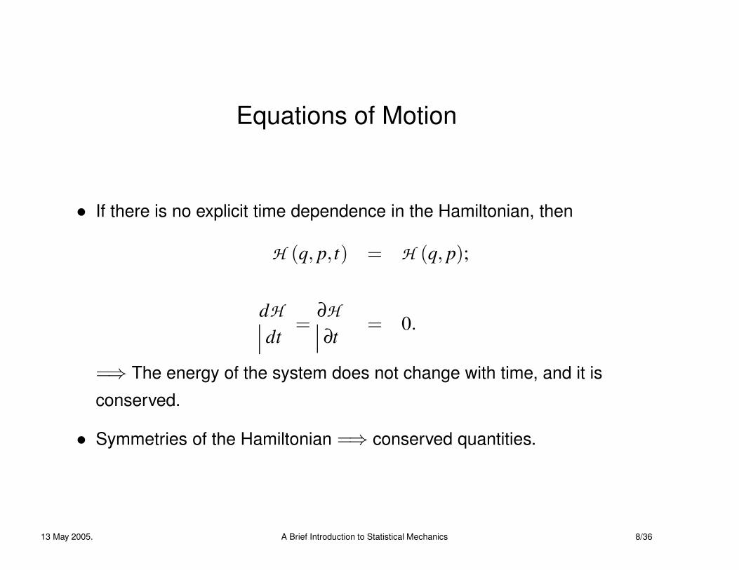
Equations of Motion
• If there is no explicit time dependence in the Hamiltonian, then
H (q, p, t) = H (q, p);
dHdt
=∂H∂t
= 0.
=⇒ The energy of the system does not change with time, and it is
conserved.
• Symmetries of the Hamiltonian =⇒ conserved quantities.
13 May 2005. A Brief Introduction to Statistical Mechanics 8/36
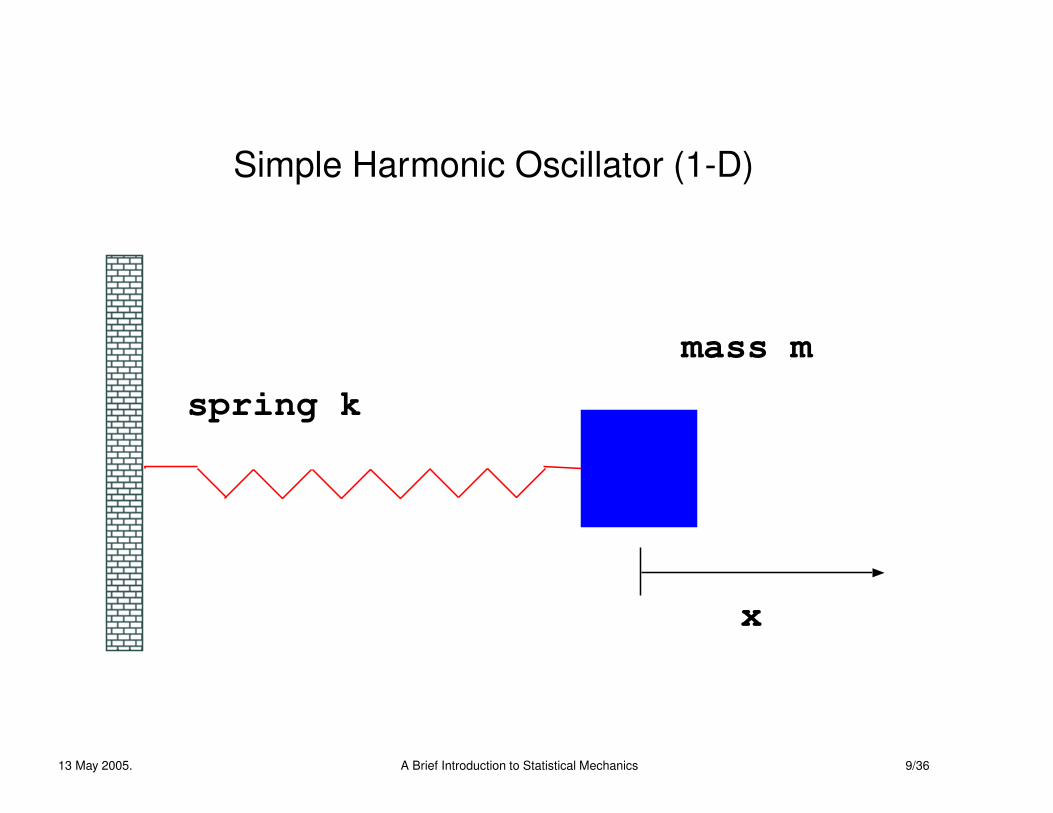
Simple Harmonic Oscillator (1-D)
x
mass m
spring k
13 May 2005. A Brief Introduction to Statistical Mechanics 9/36

Example: Simple Harmonic Oscillator (1-D)
• Consider a block of mass m connected by a spring with spring
constant k.
• Its displacement is given by x, has velocity v, momentum p = mv.
• One generalized co-ordinate x, its conjugate momentum p.
• The total energy : kinetic energy + potential energy
E =12
mv2 +12
k x2.
13 May 2005. A Brief Introduction to Statistical Mechanics 10/36
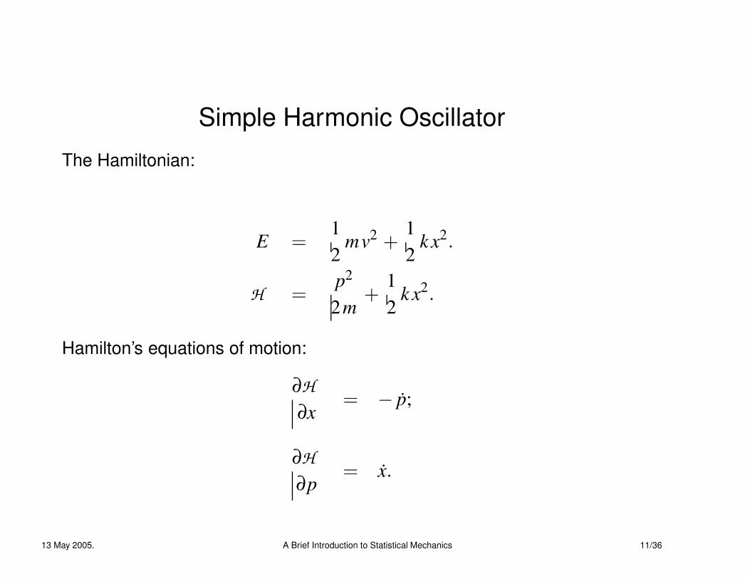
Simple Harmonic Oscillator
The Hamiltonian:
E =12
mv2 +12
k x2.
H =p2
2m+
12
k x2.
Hamilton’s equations of motion:
∂H∂x
= − p;
∂H∂p
= x.
13 May 2005. A Brief Introduction to Statistical Mechanics 11/36

Simple Harmonic Oscillator
k x = − p;pm
= x;
Rearrange, two first order ODEs:
d pd t
= −k x ; Newton’s Law
d xd t
=pm
.
Can get the usual second order ODE:
d2 xd t2 +
km
x = 0.
13 May 2005. A Brief Introduction to Statistical Mechanics 12/36
Thermodynamics
• Thermodynamics: phenomenological and empirical.
• A thermodynamic system: any macroscopic system.
• Thermodynamic parameters (state variables): measurable quantities
such as pressure P, volume V , temperature T , magnetic field H.
• A thermodynamic state is specified by particular values of P,V,T,H...
• An equation of state: a functional relation between the state
variables. Example: for an ideal gas, PV = nRT .
• Other thermodynamic quantities: internal energy E , entropy S,
specific heats CV ,CP (response functions).
13 May 2005. A Brief Introduction to Statistical Mechanics 13/36

Thermodynamics• At equilibrium, observe average behaviour.
• The internal energy E = average total energy of the system : < H >.
• Intensive and Extensive variables.
• Intensive variables do not depend on the size of the system.Examples: pressure P, temperature T , chemical potential µ.
• Extensive variables depend on the size of the system. Examples: thetotal number of particles N, volume V , internal energy E , entropy S.
• The first law of thermodynamics: energy conservation:change in internal energy = heat supplied - work done by the system.Mathematically:
dE = T dS − PdV + µ dN .
13 May 2005. A Brief Introduction to Statistical Mechanics 14/36
Thermodynamics
• T , P, µ are generalized forces, intensive. Each associated with an
extensive variable, such that
change in internal energy = generalized force × change in extensive
variable.
• {T,S}, {−P,V}, {µ,N} are conjugate variable pairs.
• Thermodynamic potentials: analogous to the mechanical potential
energy. Energy available to do work – ‘free energy’. The free energy
is minimized, depending on the conditions.
13 May 2005. A Brief Introduction to Statistical Mechanics 15/36
Thermodynamics
• Helmholtz free energy:
F = E − T S ;
dF = dE − T dS − SdT
= T dS − PdV + µ dN − T dS − SdT
dF = −PdV − SdT + µ dN .
• Like E , the potentials contain all thermodynamic information.
• Equation of state from the free energy – relates state variables:
P(V,T,N) = −∂F∂V
∣
∣
∣
∣
T,N.
13 May 2005. A Brief Introduction to Statistical Mechanics 16/36

Kinetic Theory
• A dilute gas of a large number N of molecules in a volume V .
• The temperature T is high, the density is low.
• The molecules interact via collisions.
• An isolated system will always reach equilibrium by minimizing its
energy. At equilibrium its energy does not change with time.
• Consider, for each molecule, {r, p}: 3 spatial coordinates, 3 momenta.
• Each particle corresponds to a point in a 6-D phase space.
The system as a whole can be represented as N points.
• Not interested in the detailed behaviour of each molecule.
13 May 2005. A Brief Introduction to Statistical Mechanics 17/36

Kinetic Theory – 6-D Phase Space
3 coordinates (x,y,z)
3 momenta (px,py,pz)
N points
13 May 2005. A Brief Introduction to Statistical Mechanics 18/36
Kinetic Theory
• Define a distribution function f (r, p, t) so that
f (r, p, t) dr dp
gives the number of molecules at time t lying within a volume element
dr about r and with momenta in a momentum-space volume dp about
p.
• f (r, p, t) is just the density of points in phase space.
• Assume that f is a smoothly varying continuous function, so that:Z
f (r, p, t) dr dp = N.
13 May 2005. A Brief Introduction to Statistical Mechanics 19/36

Kinetic Theory
• Problem of Kinetic Theory: Find f for given kinds of collisions (binary,
for example) – can be considered to be a form of interaction.
• Explicit expressions for pressure, temperature; temperature is a
measure of the average kinetic energy of the molecules.
• The limiting form of f as t → ∞ will yield all the equilibrium properties
for the system, and hence the thermodynamics.
• Maxwell–Boltzmann distribution of speeds for an ideal gas at
equilibrium at a given temperature: Gaussian.
• Find the time-evolution equation for f - the equation of motion in
phase space.
• Very messy!
13 May 2005. A Brief Introduction to Statistical Mechanics 20/36
Ensembles and Statistical Mechanics
• Gibbs introduced the concept of an ensemble.
• Earlier: N particles in the 6-D phase space.
• Ensemble: A single point in 6N-dimensional phase space represents
a given configuration.
• A given macrostate with {E,T,P,V, . . .} corresponds to an ensemble
of microstates: ‘snapshots’ of the system at different times.
• Ergodic hypothesis: Given enough time, the system explores all
possible points in phase space.
13 May 2005. A Brief Introduction to Statistical Mechanics 21/36

Ensemble Theory – 6N-D Phase Space
3 N coordinates
3 N momenta 1 point
Ensemble
13 May 2005. A Brief Introduction to Statistical Mechanics 22/36

Ensembles and Statistical Mechanics
• Central idea: replace time averages by ensemble averages.
• Time Average: For any quantity φ(r,p, t):
< φ(r,p, t) >=1τ
Z τ
0φ(r,p, t) dt.
• Ensemble Average: For τ → ∞:
< φ(r,p, t) >=
Z
ρ(r,p) φ(r,p, t) drdp.
dr = dr1 dr2 . . . . . .drN ;
dp = dp1 dp2 . . . . . .dpN .
13 May 2005. A Brief Introduction to Statistical Mechanics 23/36

Ensembles
• ρ(r,p): probability density,
ρ(r,p) dr dp : probability of finding the system in a volume element
[dr dp] around (r,p).
• Different ensembles: microcanonical, canonical and grandcanonical ensembles.
• Microcanonical ensemble: isolated systems with fixed energy and
number of particles, no exchange of energy or particles with the
outside world. Not very useful !
13 May 2005. A Brief Introduction to Statistical Mechanics 24/36
Ensembles
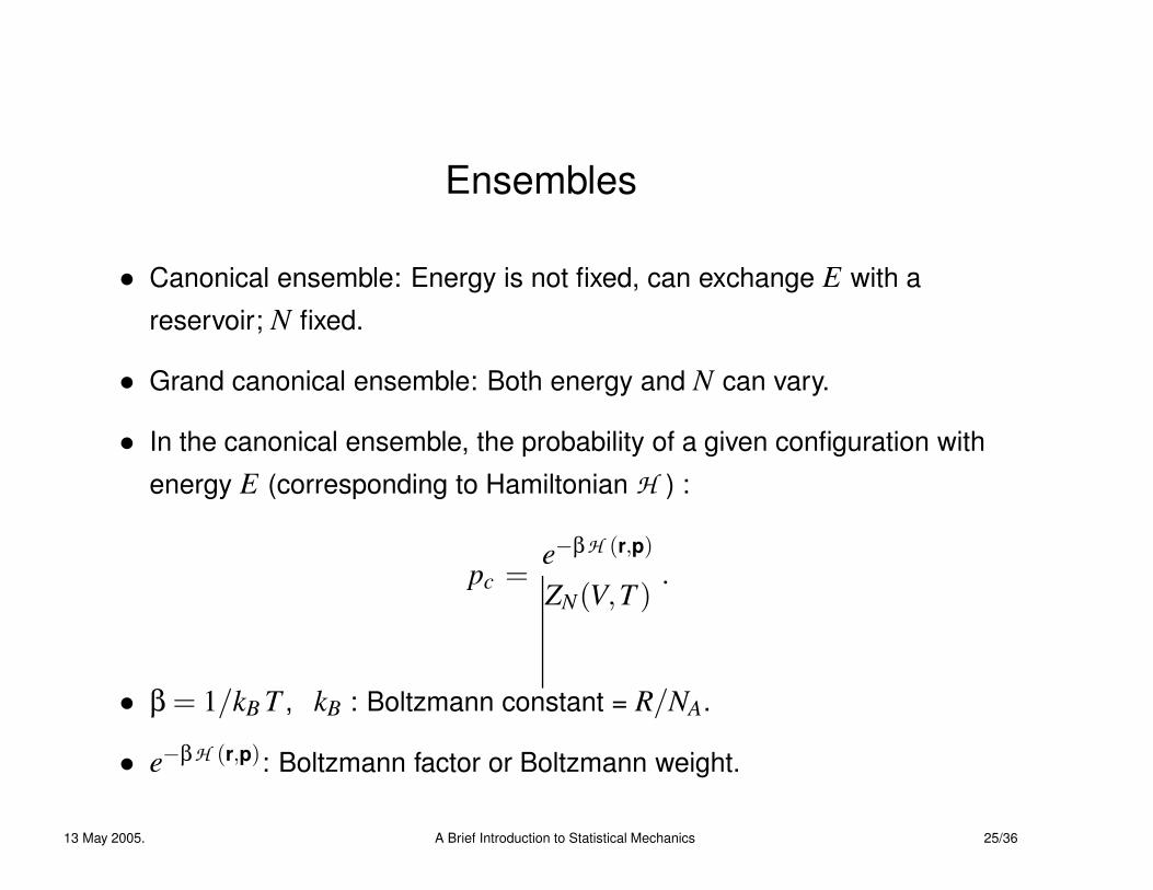
• Canonical ensemble: Energy is not fixed, can exchange E with a
reservoir; N fixed.
• Grand canonical ensemble: Both energy and N can vary.
• In the canonical ensemble, the probability of a given configuration with
energy E (corresponding to Hamiltonian H ) :
pc =e−βH (r,p)
ZN(V,T ).
• β = 1/kB T , kB : Boltzmann constant = R/NA.
• e−βH (r,p): Boltzmann factor or Boltzmann weight.
13 May 2005. A Brief Introduction to Statistical Mechanics 25/36

The Canonical Partition Function
ZN(V,T ) =1
N! h3N
Z
dr dp e−βH (r,p)
h: Planck’s constant.
• ZN : phase space volume, each volume element weighted with the
Boltzmann factor.
• From ZN , we can calculate various thermodynamic quantities.
13 May 2005. A Brief Introduction to Statistical Mechanics 26/36
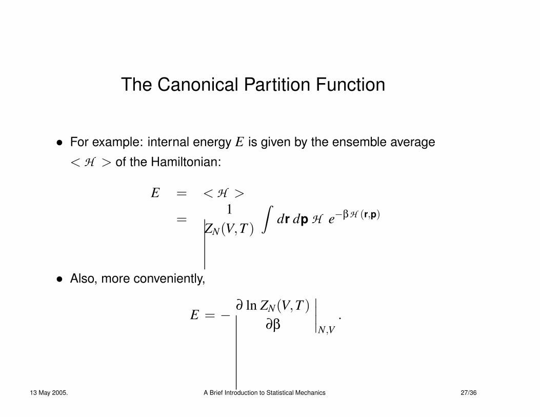
The Canonical Partition Function
• For example: internal energy E is given by the ensemble average
< H > of the Hamiltonian:
E = < H >
=1
ZN(V,T )
Z
dr dp H e−βH (r,p)
• Also, more conveniently,
E = −∂ ln ZN(V,T )
∂β
∣
∣
∣
∣
N,V.
13 May 2005. A Brief Introduction to Statistical Mechanics 27/36
The Canonical Partition Function
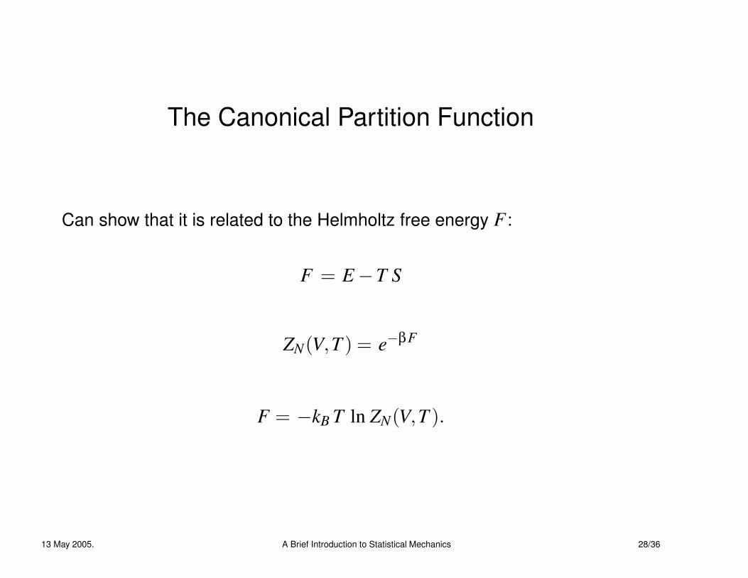
Can show that it is related to the Helmholtz free energy F :
F = E −T S
ZN(V,T ) = e−βF
F = −kB T ln ZN(V,T ).
13 May 2005. A Brief Introduction to Statistical Mechanics 28/36
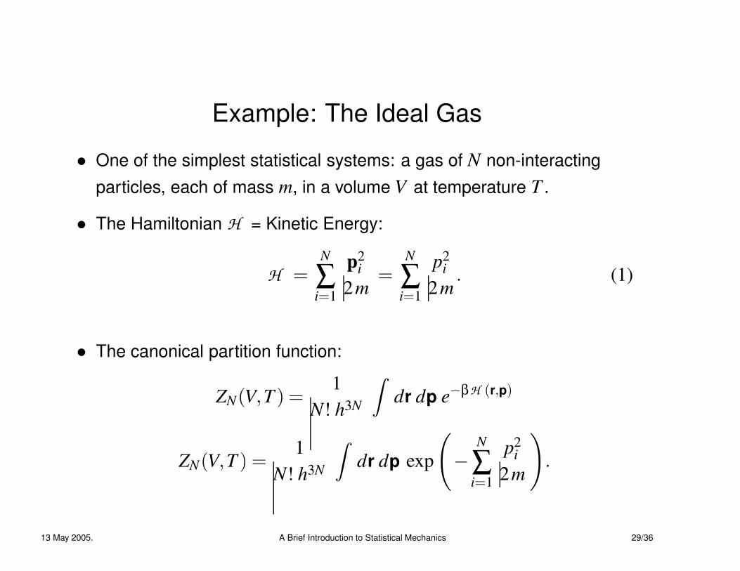
Example: The Ideal Gas
• One of the simplest statistical systems: a gas of N non-interactingparticles, each of mass m, in a volume V at temperature T .
• The Hamiltonian H = Kinetic Energy:
H =N
∑i=1
p2i
2m=
N
∑i=1
p2i
2m. (1)
• The canonical partition function:
ZN(V,T ) =1
N! h3N
Z
dr dp e−βH (r,p)
ZN(V,T ) =1
N! h3N
Z
dr dp exp
(
−N
∑i=1
p2i
2m
)
.
13 May 2005. A Brief Introduction to Statistical Mechanics 29/36

Example: The Ideal Gas
ZN =V N
N! h3N
(
Z ∞
−∞d p e−β p2/2m
)3N
ZN =V N
N! h3N
(
√
2πm/β)3N
=V N
N! h3N (2πmkB T )3N/2
ln ZN = N lnV +32
N [ ln(2πm)− lnβ ] − lnN! − 3N ln h .
13 May 2005. A Brief Introduction to Statistical Mechanics 30/36

The Ideal Gas
• Can calculate macroscopic thermodynamical quantities.
• Average (kinetic) energy of the gas:
E = −∂ ln ZN
∂β
= −∂(− 3
2 N lnβ)
∂β
=32
Nβ
E =32
N kB T .
• Average (kinetic) energy per particle: EN = 3
2 kB T.
13 May 2005. A Brief Introduction to Statistical Mechanics 31/36
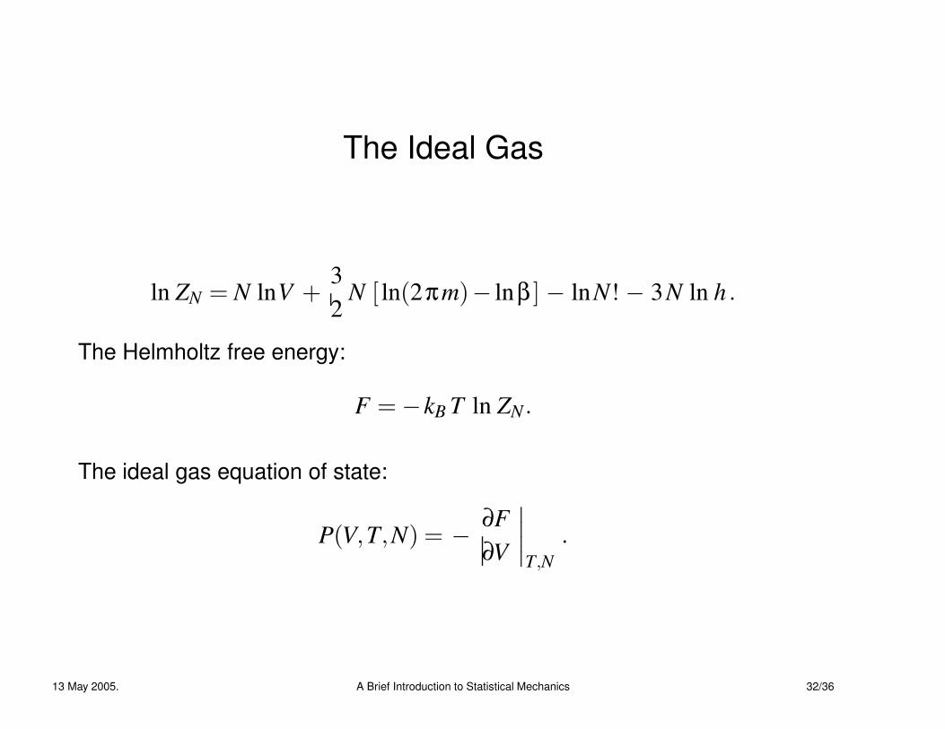
The Ideal Gas
ln ZN = N lnV +32
N [ ln(2πm)− lnβ ] − lnN! − 3N ln h .
The Helmholtz free energy:
F = −kB T ln ZN .
The ideal gas equation of state:
P(V,T,N) = −∂F∂V
∣
∣
∣
∣
T,N.
13 May 2005. A Brief Introduction to Statistical Mechanics 32/36
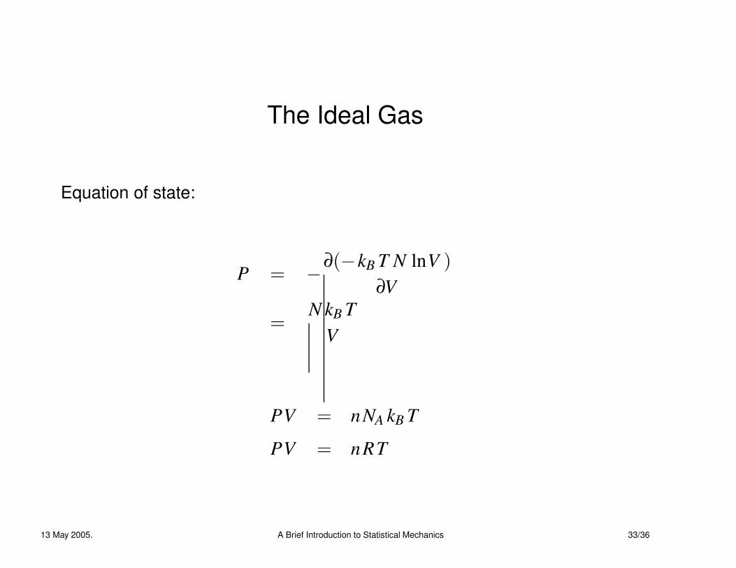
The Ideal Gas
Equation of state:
P = −∂(−kB T N lnV )
∂V
=N kB T
V
PV = nNA kB T
PV = nRT
13 May 2005. A Brief Introduction to Statistical Mechanics 33/36
The Partition Function
• The partition function approach is very important because of its
success.
• A whole range of equilibrium phenomena can be understood this way.
• Recipe: Write down the Hamiltonian - mostly interested in the
potential energy term:
V = Vext +Vint
• The Vint term includes all the interactions: two-body, three-body . . .
• Get the free energy from the partition function.
• Minimize the free energy: the equilibrium ‘ground state’ of the system.
13 May 2005. A Brief Introduction to Statistical Mechanics 34/36
Extensions ?
• The Hamiltonian can be either discrete or continuous.
• Continuous systems: concept of fields (example: density field,
magnetization field, field of interactions).
• When dealing with fields, the Hamiltonian, and the free energy,
become functionals :
H = H [φ(r, t) ]
.
• Use field theory techniques and variational calculus.
• Non-equilibrium: time-dependent Hamiltonian, dissipation =⇒
transport properties; failure of equilibrium statistical mechanics.
• Deal with time-dependent probabilities: stochastic equations.
13 May 2005. A Brief Introduction to Statistical Mechanics 35/36

Concluding Remarks
• What has all this to do with research at MSDL ?
• Look for universal features and quantify them: symmetry properties;
conservation laws ?
• Equivalent concepts to: generalized coordinates, energy, energy
minimization.
• Typical scales in a problem: length and time. Approximations based
on this.
• Map one problem onto another: reduce it to something you know
(SHO) .
• Apply the statistical mechanical approach to agents.
13 May 2005. A Brief Introduction to Statistical Mechanics 36/36