A Brief Introduction to Statistical Shape Analysis

Mikkel B. Stegmann and David Delgado Gomez∗

Informatics and Mathematical Modelling, Technical University of DenmarkRichard Petersens Plads, Building 321, DK-2800 Kgs. Lyngby, Denmark

6th March 2002

Abstract

This note aims at giving a brief introduction to the field of statistical shape analysis lookedat from an image analysis point of view. Basic techniques such as Procrustes analysis, tan-gent space projection and Principal Component Analysis (PCA) are presented and subsequentlydemonstrated and discussed in depth through a biometric case study of hands.

Prerequisites are limited to basic knowledge of linear algebra and statistics at the price of asomewhat less compact presentation. To encourage learning by exploration; images, annotationsand data reports from the hand study are made available for download.

Keywords: statistical shape analysis, landmark methods, morphometrics, Procrustes analysis,principal component analysis, multivariate statistics, biometrics, active shape models.

Contents

1 Introduction 2

2 Shapes and Landmarks 2

3 Shape Alignment 33.1 The Procrustes Shape Distance . . . . . . . . . . . . . . . . . . . . . . . . . . . . . 43.2 Generalized Procrustes Analysis . . . . . . . . . . . . . . . . . . . . . . . . . . . . . 53.3 Tangent Space Projection . . . . . . . . . . . . . . . . . . . . . . . . . . . . . . . . 5

4 Modeling Shape Variation 74.1 Principal Component Analysis . . . . . . . . . . . . . . . . . . . . . . . . . . . . . 7

5 Experiments 85.1 Data . . . . . . . . . . . . . . . . . . . . . . . . . . . . . . . . . . . . . . . . . . . . 85.2 Alignment . . . . . . . . . . . . . . . . . . . . . . . . . . . . . . . . . . . . . . . . . 105.3 Statistical Analysis . . . . . . . . . . . . . . . . . . . . . . . . . . . . . . . . . . . . 115.4 On the Practical Impact of Tangent Space Projection . . . . . . . . . . . . . . . . 14

6 Concluding Remark 14

7 Acknowledgements 14

References 15

∗Contact information: {mbs,ddg}@imm.dtu.dk, http://www.imm.dtu.dk/˜mbs/

1

1 Introduction

For exactly a decade ago the image analysis community was introduced one of the more influentialideas within the community these past ten years. The paper giving name to this idea borrowedattention from the much famous Snakes paper [15] by Kass, Witkin and Terzopoulos and waspublished in 1992 as Active Shape Models – ’Smart Snakes’ [4] and the later major introductionas Active Shape Models - their training and application [6] by T. F. Cootes, C. J. Taylor, D. H.Cooper and J. Graham in 1995. The brotherhood with Snakes was rightfully claimed as theyboth are deformable models but contrary to Snakes, Active Shape Models (ASMs) have globalconstraints w.r.t. shape. These constraints are learned though observation giving the model flex-ibility, robustness and specificity as the model only can synthesize plausible instances w.r.t. theobservations.

This note introduces the foundation of Active Shape Models1, namely the statistical analysisof shapes – a discipline that dates back to the work of Sir D’Arcy Wentworth Thompson [19] –which is widely applicable to many other areas than image analysis. For further readings we havea few pointers into the vast amount of literature [7, 11, 1, 10, 5, 17].

2 Shapes and Landmarks

What do we actually understand by the concept of shape? In this text we will adapt the definitionby D.G. Kendall [7]:

Definition 1 : Shape is all the geometrical information that remains when location,scale and rotational effects are filtered out from an object.

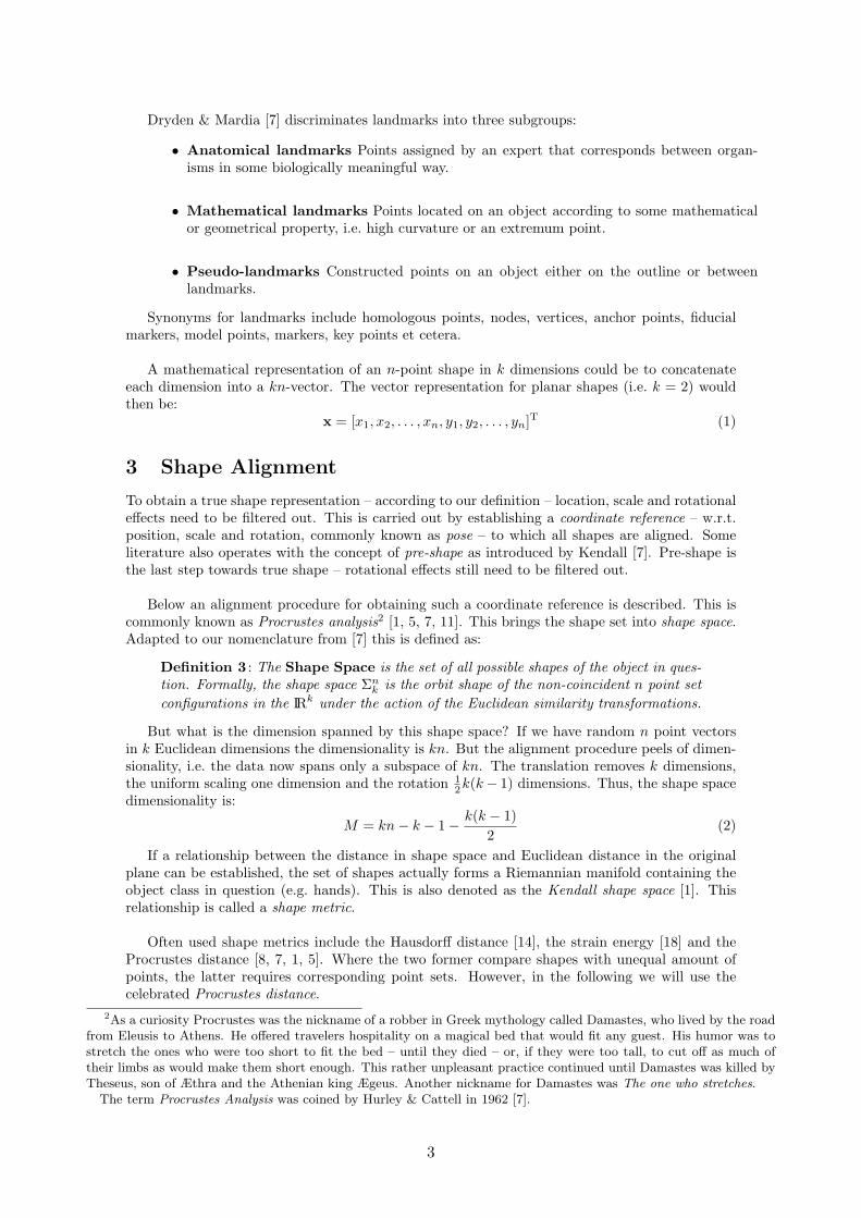
According to this shape is – in other words – invariant to Euclidean similarity transformations.This is reflected in fig. 1. The next question that naturally arises is: How should one describea shape? In everyday conversation, unknown shapes are often described as references to knownshapes – e.g. ”Italy has the shape of a boot”. Such descriptions can obviously not easily be utilizedin an algorithmic framework.

Figure 1: Four copies of the same shape, but under different Euclidean transformations.

One way to describe a shape is by locating a finite number of points on the outline. Conse-quently, the concept of a landmark is adapted [7]:

Definition 2 : A landmark is a point of correspondence on each object that matchesbetween and within populations.

1Beside ASMs statistical shape analysis is also the foundation the myriads of models [6] spawned, most notably theActive Appearance Models [9, 2, 3].

2

Dryden & Mardia [7] discriminates landmarks into three subgroups:

• Anatomical landmarks Points assigned by an expert that corresponds between organ-isms in some biologically meaningful way.

• Mathematical landmarks Points located on an object according to some mathematicalor geometrical property, i.e. high curvature or an extremum point.

• Pseudo-landmarks Constructed points on an object either on the outline or betweenlandmarks.

Synonyms for landmarks include homologous points, nodes, vertices, anchor points, fiducialmarkers, model points, markers, key points et cetera.

A mathematical representation of an n-point shape in k dimensions could be to concatenateeach dimension into a kn-vector. The vector representation for planar shapes (i.e. k = 2) wouldthen be:

x = [x1, x2, . . . , xn, y1, y2, . . . , yn]T (1)

3 Shape Alignment

To obtain a true shape representation – according to our definition – location, scale and rotationaleffects need to be filtered out. This is carried out by establishing a coordinate reference – w.r.t.position, scale and rotation, commonly known as pose – to which all shapes are aligned. Someliterature also operates with the concept of pre-shape as introduced by Kendall [7]. Pre-shape isthe last step towards true shape – rotational effects still need to be filtered out.

Below an alignment procedure for obtaining such a coordinate reference is described. This iscommonly known as Procrustes analysis2 [1, 5, 7, 11]. This brings the shape set into shape space.Adapted to our nomenclature from [7] this is defined as:

Definition 3 : The Shape Space is the set of all possible shapes of the object in ques-tion. Formally, the shape space Σn

k is the orbit shape of the non-coincident n point setconfigurations in the IRk under the action of the Euclidean similarity transformations.

But what is the dimension spanned by this shape space? If we have random n point vectorsin k Euclidean dimensions the dimensionality is kn. But the alignment procedure peels of dimen-sionality, i.e. the data now spans only a subspace of kn. The translation removes k dimensions,the uniform scaling one dimension and the rotation 1

2k(k− 1) dimensions. Thus, the shape spacedimensionality is:

M = kn− k − 1− k(k − 1)2

(2)

If a relationship between the distance in shape space and Euclidean distance in the originalplane can be established, the set of shapes actually forms a Riemannian manifold containing theobject class in question (e.g. hands). This is also denoted as the Kendall shape space [1]. Thisrelationship is called a shape metric.

Often used shape metrics include the Hausdorff distance [14], the strain energy [18] and theProcrustes distance [8, 7, 1, 5]. Where the two former compare shapes with unequal amount ofpoints, the latter requires corresponding point sets. However, in the following we will use thecelebrated Procrustes distance.

2As a curiosity Procrustes was the nickname of a robber in Greek mythology called Damastes, who lived by the roadfrom Eleusis to Athens. He offered travelers hospitality on a magical bed that would fit any guest. His humor was tostretch the ones who were too short to fit the bed – until they died – or, if they were too tall, to cut off as much oftheir limbs as would make them short enough. This rather unpleasant practice continued until Damastes was killed byTheseus, son of Æthra and the Athenian king Ægeus. Another nickname for Damastes was The one who stretches.

The term Procrustes Analysis was coined by Hurley & Cattell in 1962 [7].

3

3.1 The Procrustes Shape Distance

The Procrustes distance is a least-squares type shape metric that requires two aligned shapes withone-to-one point correspondence. The alignment part involves four steps:

1. Compute the centroid of each shape.

2. Re-scale each shape to have equal size.

3. Align w.r.t. position the two shapes at their centroids.

4. Align w.r.t. orientation by rotation.

Now, the squared Procrustes distance between two shapes, x1 and x2, is simply the sum ofthe squared point distances:

P 2d =

n∑

j=1

[(xj1 − xj2)2 + (yj1 − yj2)

2] (3)

Since the centroid of a shape is the center of mass of the physical system consisting of unitmasses at each landmark, this is easily calculated as:

(x, y) =

1

n

n∑

j=1

xj ,1n

n∑

j=1

yj

(4)

To perform step two we obviously need to establish a shape size metric:

Definition 4 : A shape size metric S(x) is any positive real valued function of theshape vector that fulfils the following property (like all other metrics):

S(ax) = aS(x)

In the following the Frobenius norm (or 2-norm) is used as a shape size metric:

S(x) =

√√√√n∑

j=1

[(xj − x)2 + (yj − y)2] (5)

Another often used scale metric is the centroid size:

S(x) =n∑

j=1

√(xj − x)2 + (yj − y)2 (6)

This metric also posses the interesting property that 2nS(x)2 equals the sum of the inter-landmark distances [7].

Turning to step three a Singular Value Decomposition (SVD) is applied [1]:

1. Arrange the size and position aligned x1 and x2 as n×k matrices (in the planar case k = 2).

2. Calculate the SVD, UDVT, of xT1 x2 in order to maximize the correlation between the two

sets of landmarks.

3. The rotation matrix needed to optimally superimpose x1 upon x2 is then VUT:

VUT =[

cos(θ) − sin(θ)sin(θ) cos(θ)

](7)

4

3.2 Generalized Procrustes Analysis

All though an analytic solution exists [12, 7] to the alignment of a set of planar shapes the followingiterative approach to generalized Procrustes analysis [1, 5] will suffice.

1. Choose an initial estimate of the mean shape (e.g. the first shape in the set).

2. Align all the remaining shapes to the mean shape.

3. Re-calculate the estimate of the mean from the aligned shapes.

4. If the estimated mean has changed return to step 2.

Convergence is thus declared when the mean shape does not change significantly within aniteration. Bookstein [1] notes that two iterations of the above should be sufficient in most cases.

The remaining question is how to obtain an estimate of the mean shape (or shape prototype).The most frequently used is the Procrustes mean shape or just the Procrustes mean (also referredto as the Frechet mean). Let N denote the number of shapes, then the Procrustes mean is:

x =1N

N∑

i=1

xi (8)

Further, to avoid any shrinking or drifting of the mean shape – size and orientation should beproperly fixed at each iteration by normalization.

Now, lets return to the concept of a manifold introduced earlier. Due to the size normalizationall shape vectors live on a subpart of an kn-dimensional hyper sphere. This hyper sphere representsall shapes of k landmarks in n Euclidean dimensions, but the subpart in question represents onlyshapes of the object class in question, e.g. hand outlines. This subpart constitutes the so-calledmanifold.

3.3 Tangent Space Projection

It is a fact that linear methods are nice. Well-behaved, have good performance where applicableand very well understood. However, these stand in striking contrast to the curved surface of highdimensional produced by the Procrustes analysis. This is the (partial) aim of a tangent spaceprojection. Modifying the shape vectors to form a hyper plane, instead of a subpart of a hypersphere. Further, the Euclidean distance in this plane can be employed as shape metric instead ofthe true geodesic distance, i.e at the hyper sphere surface.

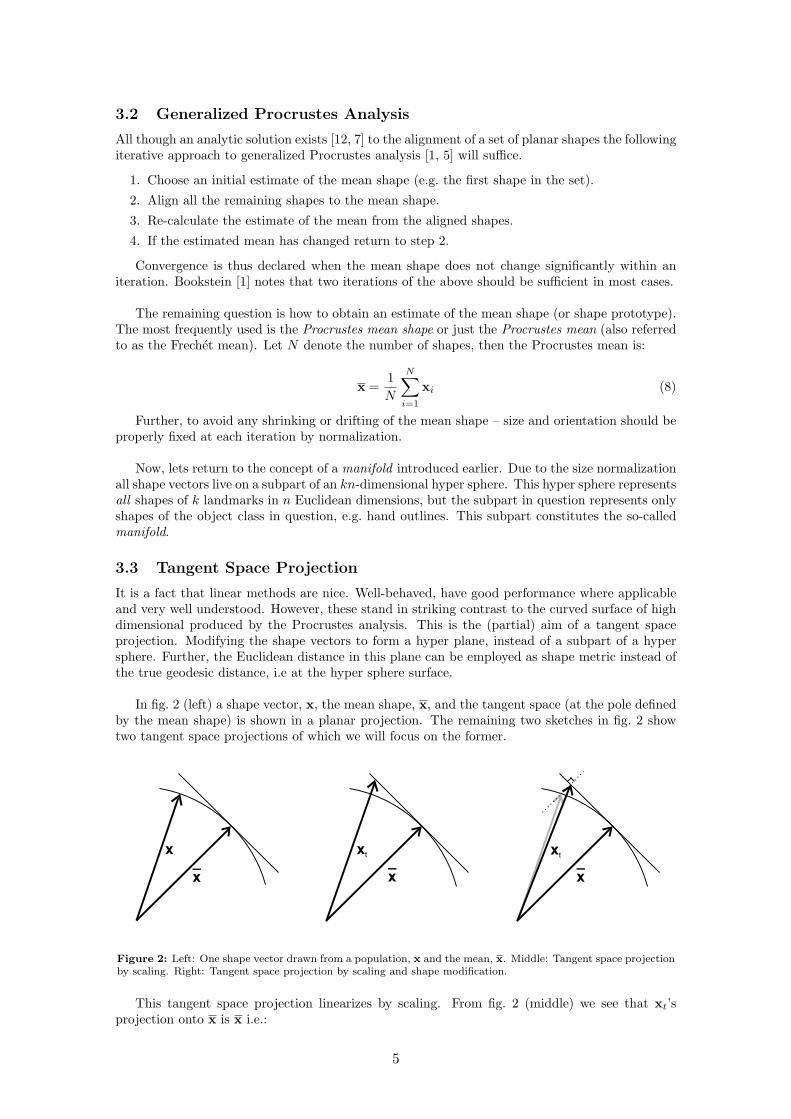
In fig. 2 (left) a shape vector, x, the mean shape, x, and the tangent space (at the pole definedby the mean shape) is shown in a planar projection. The remaining two sketches in fig. 2 showtwo tangent space projections of which we will focus on the former.

Figure 2: Left: One shape vector drawn from a population, x and the mean, x. Middle: Tangent space projectionby scaling. Right: Tangent space projection by scaling and shape modification.

This tangent space projection linearizes by scaling. From fig. 2 (middle) we see that xt’sprojection onto x is x i.e.:

5

x =x · xt

|x|2 x = βx (9)

Substituting xt with αx in the scaling factor, β, we get:

β = 1 =x · xt

|x|2 = αx · x|x|2 (10)

And finally

xt = αx =|x|2x · xx (11)

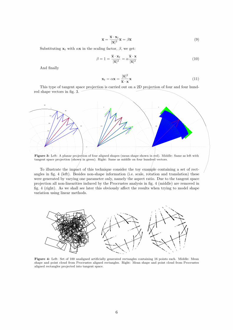
This type of tangent space projection is carried out on a 2D projection of four and four hund-red shape vectors in fig. 3.

0.2

0.4

0.6

0.8

1

30

60

90

0

0.5

1

0.5

1

Figure 3: Left: A planar projection of four aligned shapes (mean shape shown in red). Middle: Same as left withtangent space projection (shown in green). Right: Same as middle on four hundred vectors.

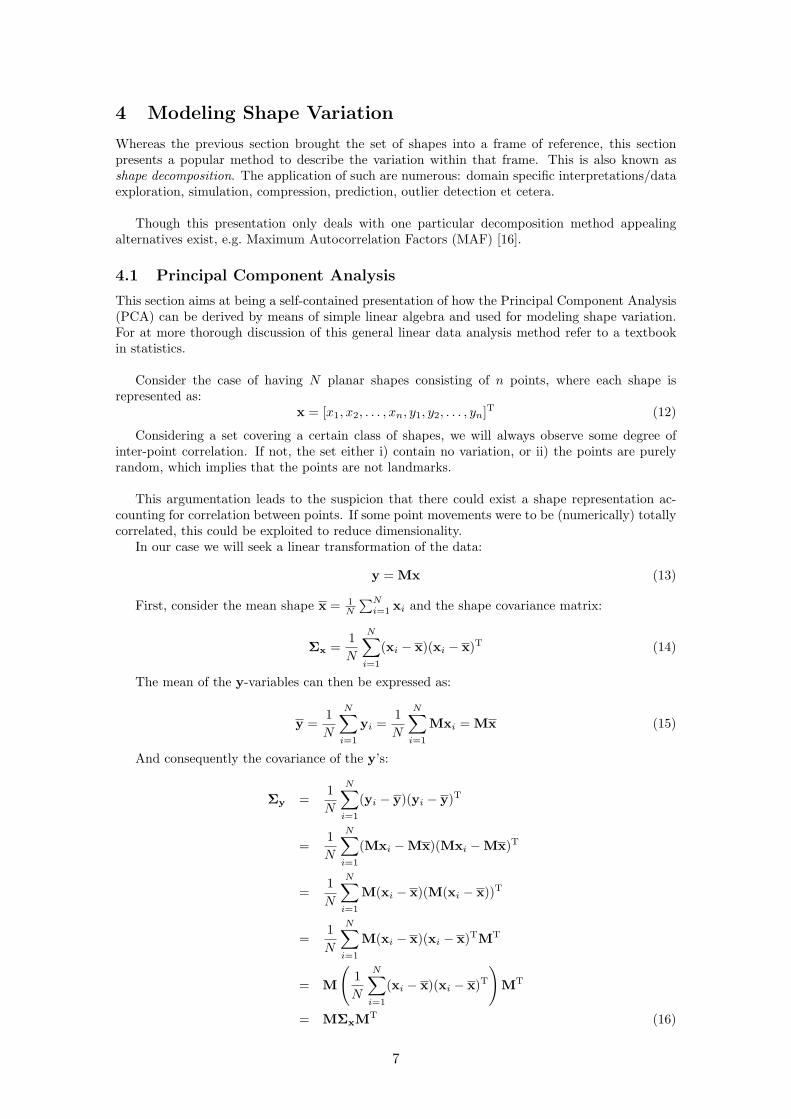
To illustrate the impact of this technique consider the toy example containing a set of rect-angles in fig. 4 (left). Besides non-shape information (i.e. scale, rotation and translation) thesewere generated by varying one parameter only, namely the aspect ratio. Due to the tangent spaceprojection all non-linearities induced by the Procrustes analysis in fig. 4 (middle) are removed infig. 4 (right). As we shall see later this obviously affect the results when trying to model shapevariation using linear methods.

Figure 4: Left: Set of 100 unaligned artificially generated rectangles containing 16 points each. Middle: Meanshape and point cloud from Procrustes aligned rectangles. Right: Mean shape and point cloud from Procrustesaligned rectangles projected into tangent space.

6

4 Modeling Shape Variation

Whereas the previous section brought the set of shapes into a frame of reference, this sectionpresents a popular method to describe the variation within that frame. This is also known asshape decomposition. The application of such are numerous: domain specific interpretations/dataexploration, simulation, compression, prediction, outlier detection et cetera.

Though this presentation only deals with one particular decomposition method appealingalternatives exist, e.g. Maximum Autocorrelation Factors (MAF) [16].

4.1 Principal Component Analysis

This section aims at being a self-contained presentation of how the Principal Component Analysis(PCA) can be derived by means of simple linear algebra and used for modeling shape variation.For at more thorough discussion of this general linear data analysis method refer to a textbookin statistics.

Consider the case of having N planar shapes consisting of n points, where each shape isrepresented as:

x = [x1, x2, . . . , xn, y1, y2, . . . , yn]T (12)

Considering a set covering a certain class of shapes, we will always observe some degree ofinter-point correlation. If not, the set either i) contain no variation, or ii) the points are purelyrandom, which implies that the points are not landmarks.

This argumentation leads to the suspicion that there could exist a shape representation ac-counting for correlation between points. If some point movements were to be (numerically) totallycorrelated, this could be exploited to reduce dimensionality.

In our case we will seek a linear transformation of the data:

y = Mx (13)

First, consider the mean shape x = 1N

∑Ni=1 xi and the shape covariance matrix:

Σx =1N

N∑

i=1

(xi − x)(xi − x)T (14)

The mean of the y-variables can then be expressed as:

y =1N

N∑

i=1

yi =1N

N∑

i=1

Mxi = Mx (15)

And consequently the covariance of the y’s:

Σy =1N

N∑

i=1

(yi − y)(yi − y)T

=1N

N∑

i=1

(Mxi −Mx)(Mxi −Mx)T

=1N

N∑

i=1

M(xi − x)(M(xi − x))T

=1N

N∑

i=1

M(xi − x)(xi − x)TMT

= M

(1N

N∑

i=1

(xi − x)(xi − x)T)

MT

= MΣxMT (16)

7

Then, if we limit ourselves to orthogonal transformations (i.e. M−1 = MT) left-multiplicationby MT in (16) yields:

MTΣy = ΣxMT (17)

Substitution of MT by Φ yields:ΣxΦ = ΦΣy (18)

From (18) it is seen that if Φ is chosen as the (column) eigenvectors of the symmetric matrixΣx, then the covariance of the transformed shapes, Σy, becomes a diagonal matrix of eigenvalues.In the case of correlated points the smallest eigenvalues will be (close to) zero and the correspond-ing eigenvectors could be omitted from Φ, thus reducing the length of y.

In conclusion, to establish a linear transform that de-correlate data vectors, the transformationmatrix must be the eigenvectors of the covariance matrix of the original data. In order to backtransform from the new set of variables, y, we invert (13), remembering that M is orthogonal:

x = M−1y = MTy = Φy (19)

Typically one would apply PCA on variables with zero mean (notice that the Φ is unchanged):

y = M(x− x) , x = x + Φx (20)

This celebrated method of dealing with redundancy in multivariate data is known as PrincipalComponent Analysis (PCA) or the Karhunen-Loeve Transform (KLT). It was introduced back in1933 by Harold Hotelling [13] based on work by Karl Pearson.

It should be mentioned that the PCA also could be derived as a variance maximizing changeof basis given an orthonormality constraint using a Lagrange formulation. Not surprisingly thesolution of this constrained optimization problem leads to the same eigenproblem as above.

Returning to fig. 4 PCA on the raw aligned rectangles (middle) decomposes the variation intotwo components accounting for 99.6% and 0.4% of the total variation, respectively. Knowing thatonly the aspect ratio changes this seems unsatisfactory.3 However, linearizing by a tangent spaceprojection, fig. 4 (right), the PCA can decompose all variation using one component.

5 Experiments

To demonstrate the techniques described above, this section provides a case study along with anin-depth discussion of the results. All results should be easily reproduced with Matlab, R, S-Plusor a similar using the annotations available from the internet.4

5.1 Data

The foundation for all subsequent analysis is 40 images of human hands record using an OlympusC-2040 digital camera at a resolution of 1600×1200 pixels. Four people contributed with tenimages each of their left hand. The first six of each ten were constructed as an equally spacedsequence from maximally to minimally spread fingers. The remaining four were chosen arbitrarilyby the test persons under the constraints i) that the palm should face the support and ii) thatthe hand contour should represent a simple curve (i.e. no crossings).

3From a theoretically point of view that is. From a numerically point of view one would discard the small componentintroduced by the non-linearity.

4Annotations, images and data reports may be obtained from http://www.imm.dtu.dk/~mbs/.

8

1

2

3

4

5

6 7 8

9

10

11

12 13

14 15 16 17

18 19

20 21 22

23 24

25 26 27 28 29 30 31 32 33

34

35 36 37 38 39 40 41

42 43

44

45 46

47 48 49 50

51

52

53 54 55

56

Figure 5: Annotated hand using 56 landmarks.

1

2 3 4 5 6 7

8

9 10 11 12 13

14 15 16 17 18 19 20 21 22 23 24 25 26 27

28 29 30 31 32 33 34 35 36 37

38 39 40 41 42 43 44 45 46 47 48

49 50 51 52 53 54 55

56

Figure 6: Annotated hand with contracted fingers.

9

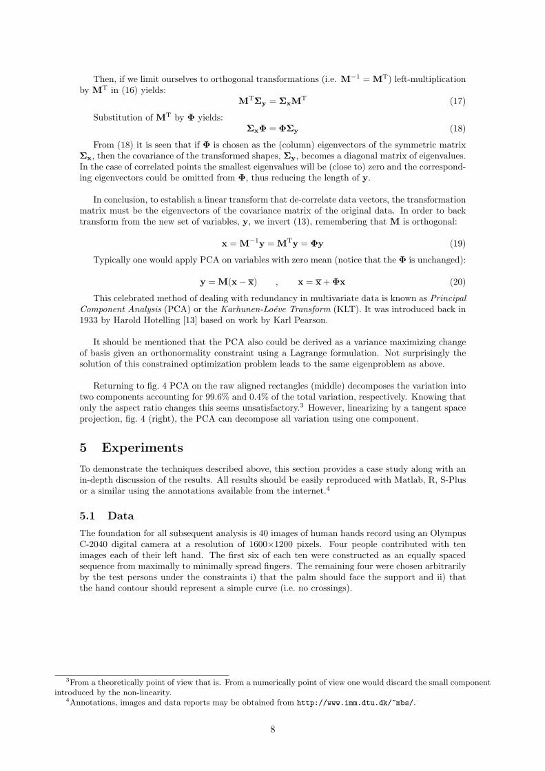
The set of images was brought into correspondence by placing 56 landmarks upon the contourof the hand. An example is given in fig. 5. The distribution of landmarks is as follows:

• 43 type I landmarks (anatomical landmarks).

• 9 type II landmarks (mathematical landmarks): 8, 12, 18, 23, 28, 33, 38, 43, 48.

• 4 type III landmarks (pseudo-landmarks): 2, 11, 54, 55.

The 43 anatomical landmarks were placed i) at the border between forearm and hand, and ii)the knuckles and nails.5 The four pseudo-landmarks were placed (also by hand) to minimize thedistance from the linear spline defined by the 56 landmarks and the actual hand contour.

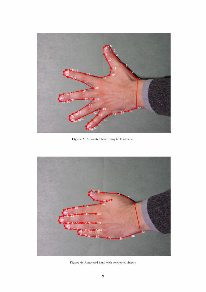
5.1.1 Remarks regarding the annotation

Specifically regarding hands, fig. 6 indicates that the landmarks 11, 12 are slightly problematicand must be placed with caution. There is further a great variability in the visibility of theknuckles, which leads to a higher uncertainty on these landmarks.

In general, one should bear in mind that placing landmarks is per se a subjective task. Foroptimal accuracy, intra- and inter-grader/annotator variability studies should be carried out (alsocalled a repeatability and reproducibility study). This is accomplished by letting a set of oper-ators annotate the data set several times each. At each annotation the image order should berandomized to remove ordering-bias. From these sets, point error variances between and withinoperators are estimated and a maximum likelihood set are estimated.

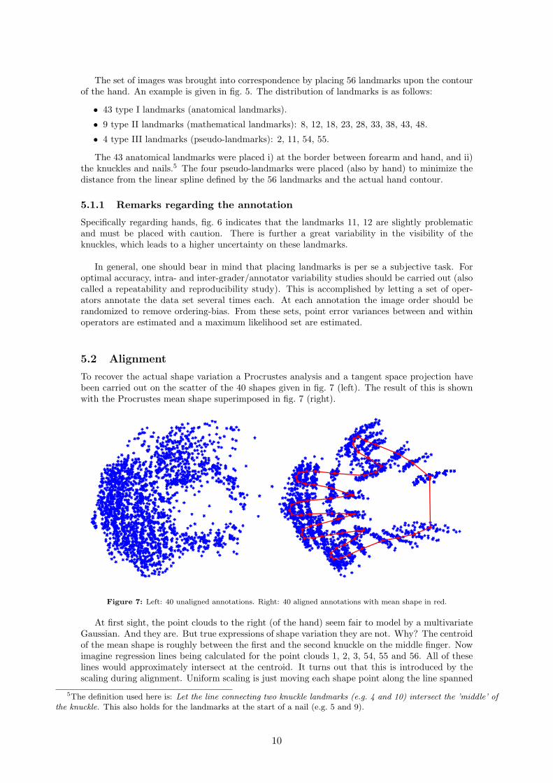
5.2 Alignment

To recover the actual shape variation a Procrustes analysis and a tangent space projection havebeen carried out on the scatter of the 40 shapes given in fig. 7 (left). The result of this is shownwith the Procrustes mean shape superimposed in fig. 7 (right).

Figure 7: Left: 40 unaligned annotations. Right: 40 aligned annotations with mean shape in red.

At first sight, the point clouds to the right (of the hand) seem fair to model by a multivariateGaussian. And they are. But true expressions of shape variation they are not. Why? The centroidof the mean shape is roughly between the first and the second knuckle on the middle finger. Nowimagine regression lines being calculated for the point clouds 1, 2, 3, 54, 55 and 56. All of theselines would approximately intersect at the centroid. It turns out that this is introduced by thescaling during alignment. Uniform scaling is just moving each shape point along the line spanned

5The definition used here is: Let the line connecting two knuckle landmarks (e.g. 4 and 10) intersect the ’middle’ ofthe knuckle. This also holds for the landmarks at the start of a nail (e.g. 5 and 9).

10

by the centroid and the point itself. The reason this occurs is that the contour is denser at thefingertips, which makes the Procrustes analysis emphasize the alignment of this part since the costis measured ’per-point’. The lesson learned here is that one should be cautious when interpretingthese scatter plots.

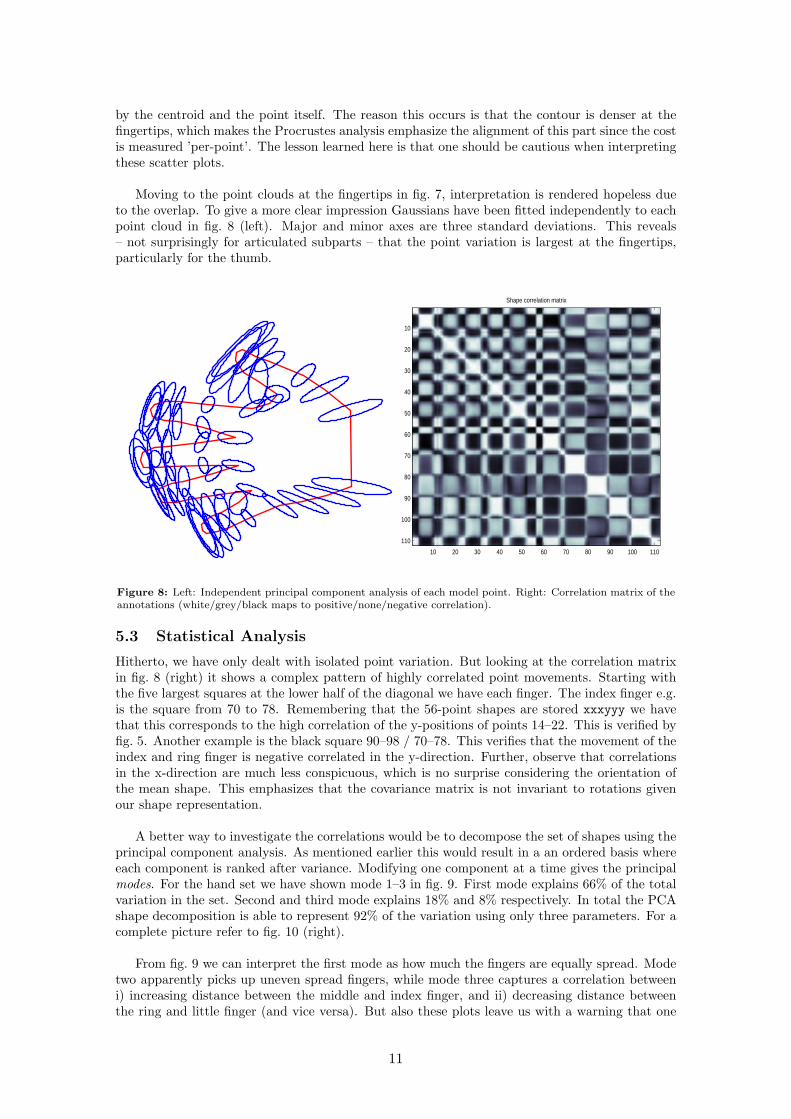
Moving to the point clouds at the fingertips in fig. 7, interpretation is rendered hopeless dueto the overlap. To give a more clear impression Gaussians have been fitted independently to eachpoint cloud in fig. 8 (left). Major and minor axes are three standard deviations. This reveals– not surprisingly for articulated subparts – that the point variation is largest at the fingertips,particularly for the thumb.

Shape correlation matrix

10 20 30 40 50 60 70 80 90 100 110

10

20

30

40

50

60

70

80

90

100

110

Figure 8: Left: Independent principal component analysis of each model point. Right: Correlation matrix of theannotations (white/grey/black maps to positive/none/negative correlation).

5.3 Statistical Analysis

Hitherto, we have only dealt with isolated point variation. But looking at the correlation matrixin fig. 8 (right) it shows a complex pattern of highly correlated point movements. Starting withthe five largest squares at the lower half of the diagonal we have each finger. The index finger e.g.is the square from 70 to 78. Remembering that the 56-point shapes are stored xxxyyy we havethat this corresponds to the high correlation of the y-positions of points 14–22. This is verified byfig. 5. Another example is the black square 90–98 / 70–78. This verifies that the movement of theindex and ring finger is negative correlated in the y-direction. Further, observe that correlationsin the x-direction are much less conspicuous, which is no surprise considering the orientation ofthe mean shape. This emphasizes that the covariance matrix is not invariant to rotations givenour shape representation.

A better way to investigate the correlations would be to decompose the set of shapes using theprincipal component analysis. As mentioned earlier this would result in a an ordered basis whereeach component is ranked after variance. Modifying one component at a time gives the principalmodes. For the hand set we have shown mode 1–3 in fig. 9. First mode explains 66% of the totalvariation in the set. Second and third mode explains 18% and 8% respectively. In total the PCAshape decomposition is able to represent 92% of the variation using only three parameters. For acomplete picture refer to fig. 10 (right).

From fig. 9 we can interpret the first mode as how much the fingers are equally spread. Modetwo apparently picks up uneven spread fingers, while mode three captures a correlation betweeni) increasing distance between the middle and index finger, and ii) decreasing distance betweenthe ring and little finger (and vice versa). But also these plots leave us with a warning that one

11

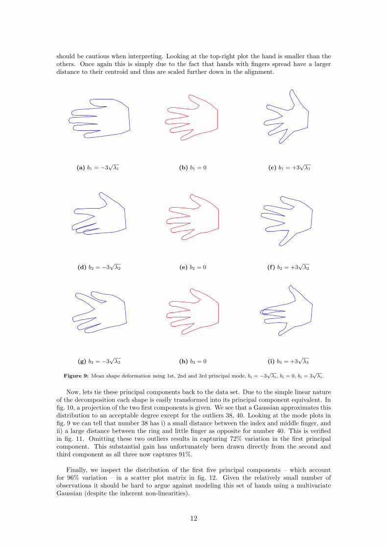
should be cautious when interpreting. Looking at the top-right plot the hand is smaller than theothers. Once again this is simply due to the fact that hands with fingers spread have a largerdistance to their centroid and thus are scaled further down in the alignment.

(a) b1 = −3√

λ1 (b) b1 = 0 (c) b1 = +3√

λ1

(d) b2 = −3√

λ2 (e) b2 = 0 (f) b2 = +3√

λ2

(g) b3 = −3√

λ3 (h) b3 = 0 (i) b3 = +3√

λ3

Figure 9: Mean shape deformation using 1st, 2nd and 3rd principal mode, bi = −3√

λi, bi = 0, bi = 3√

λi.

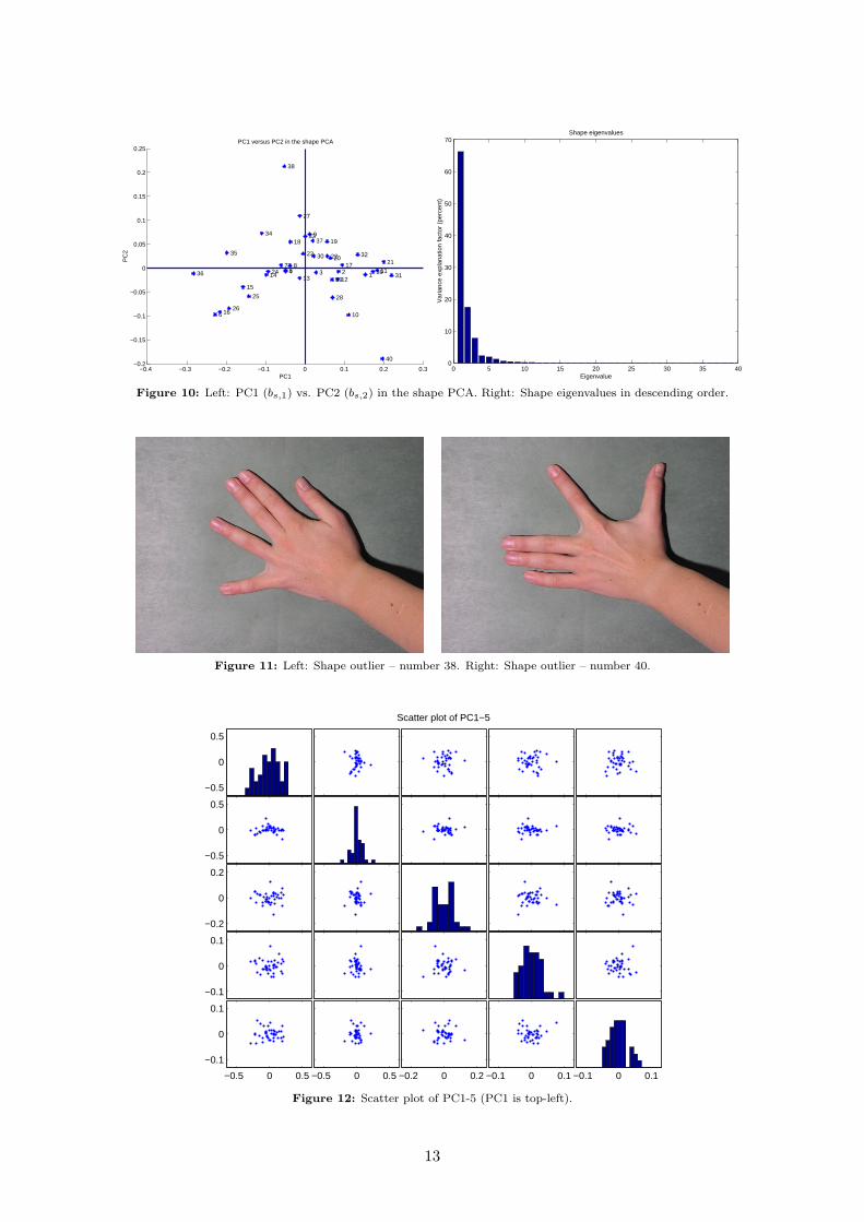
Now, lets tie these principal components back to the data set. Due to the simple linear natureof the decomposition each shape is easily transformed into its principal component equivalent. Infig. 10, a projection of the two first components is given. We see that a Gaussian approximates thisdistribution to an acceptable degree except for the outliers 38, 40. Looking at the mode plots infig. 9 we can tell that number 38 has i) a small distance between the index and middle finger, andii) a large distance between the ring and little finger as opposite for number 40. This is verifiedin fig. 11. Omitting these two outliers results in capturing 72% variation in the first principalcomponent. This substantial gain has unfortunately been drawn directly from the second andthird component as all three now captures 91%.

Finally, we inspect the distribution of the first five principal components – which accountfor 96% variation – in a scatter plot matrix in fig. 12. Given the relatively small number ofobservations it should be hard to argue against modeling this set of hands using a multivariateGaussian (despite the inherent non-linearities).

12

−0.4 −0.3 −0.2 −0.1 0 0.1 0.2 0.3−0.2

−0.15

−0.1

−0.05

0

0.05

0.1

0.15

0.2

0.25

1 2 3 4 5

6

7 8

9

10

11 12 13 14

15

16

17

18 19

20 21

22 23

24

25

26

27

28

29

30

31

32

33 34

35

36

37

38

39

40

PC1

PC

2

PC1 versus PC2 in the shape PCA

0 5 10 15 20 25 30 35 400

10

20

30

40

50

60

70

Eigenvalue

Var

ianc

e ex

plan

atio

n fa

ctor

(pe

rcen

t)

Shape eigenvalues

Figure 10: Left: PC1 (bs,1) vs. PC2 (bs,2) in the shape PCA. Right: Shape eigenvalues in descending order.

Figure 11: Left: Shape outlier – number 38. Right: Shape outlier – number 40.

Scatter plot of PC1−5

−0.1 0 0.1−0.1 0 0.1−0.2 0 0.2−0.5 0 0.5−0.5 0 0.5

−0.1

0

0.1

−0.1

0

0.1

−0.2

0

0.2

−0.5

0

0.5

−0.5

0

0.5

Figure 12: Scatter plot of PC1-5 (PC1 is top-left).

13

5.4 On the Practical Impact of Tangent Space Projection

Though the results in fig. 4 show promise, the effect of a tangent space projection is rarely thatclear. Omitting the tangent space projection in this study leaves imperceptible changes to bothmode plots and the structure of the PCA plots. Though very small there is a change in the rightdirection regarding the compactness of the shape PCA model. PC1 drops from 66.28% to 65.79%,PC2 from 17.56% to 17.51% and using five parameters the accumulated variation are 95.95% and95.56% with and without tangent space projection respectively. This scenario is typical to mostshape models built by the authors. In summary the projection is simple to apply and pleasingfrom a mathematical point of view the net effect however, is minimal from a numerical point ofview.6

6 Concluding Remark

We have aimed at serving a brief introduction to the large and intriguing field of statistical shapeanalysis in an informal and not particular mathematical manner (given the topic). The motivationfor doing so is the apparent lack of such an introduction. Techniques have been presented anddemonstrated on a data set with well known characteristics, namely hands, and by preparing thedata set and three thorough data reports along with this introduction, it is our hope that this willinspire the reader to validate the results and continue the exploration.

As the treatment of the topic is by no mean exhaustive we point to the references for all theexciting details and comments that this text left out.

7 Acknowledgements

The left hands of Panagiotis Karras, Lars Pedersen and the authors are gratefully acknowledgedfor their participation in the case study.

6We stress this is purely our opinion regarding shape modeling settings similar to this.

14

References

[1] F. L. Bookstein. Landmark methods for forms without landmarks: localizing group differ-ences in outline shape. Medical Image Analysis, 1(3):225–244, 1997.

[2] T. F. Cootes, G. J. Edwards, and C. J. Taylor. Active appearance models. In Proc. EuropeanConf. on Computer Vision, volume 2, pages 484–498. Springer, 1998.

[3] T. F. Cootes, G. J. Edwards, and C. J. Taylor. Active appearance models. IEEE Trans. onPattern Recognition and Machine Intelligence, 23(6):681–685, 2001.

[4] T. F. Cootes and Taylor. Active shape models – ’smart snakes’. In Proc. British MachineVision Conf., BMVC92, pages 266–275, 1992.

[5] T. F. Cootes and C. J Taylor. Statistical Models of Appearance for Computer Vision. Tech.Report. Oct 2001, University of Manchester, http://www.isbe.man.ac.uk/˜bim/, oct 2001.

[6] T. F. Cootes, C. J. Taylor, D. H. Cooper, and J. Graham. Active shape models - theirtraining and application. Computer Vision and Image Understanding, 61(1):38–59, 1995.

[7] I. L. Dryden and K. V. Mardia. Statistical Shape Analysis. John Wiley & Sons, 1998.

[8] N. Duta, A. K. Jain, and M.-P. Dubuisson-Jolly. Learning 2D shape models. In Proc. Conf.on Computer Vision and Pattern Recognition, volume 2, pages 8–14, 1999.

[9] G.J. Edwards, C. J. Taylor, and T. F. Cootes. Interpreting face images using active appear-ance models. In Proc. 3rd IEEE Int. Conf. on Automatic Face and Gesture Recognition,pages 300–5. IEEE Comput. Soc, 1998.

[10] Hrafkell Eiriksson. Shape represenation, alignment and decomposition. Master’s thesis,Informatics and Mathematical Modelling, Technical University of Denmark, Lyngby, 2001.

[11] C. Goodall. Procrustes methods in the statistical analysis of shape. Jour. Royal StatisticalSociety, Series B, 53:285–339, 1991.

[12] B.K.P. Horn. Closed-form solution of absolute orientation using unit quaternions. Journalof the Optical Society of America A (Optics and Image Science), 4(4):629–42, 1987.

[13] Harold Hotelling. Analysis of complex statistical variables into principal components. Journalof Educational Psychology, 24:417–441, 1933.

[14] D. P. Huttenlocher, G. A. Klanderman, and W. J. Rucklidge. Comparing images using theHausdorff distance. IEEE Trans. on Pattern Analysis and Machine Intelligence, 15(9):850–863, 1993.

[15] M. Kass, A. Witkin, and D. Terzopoulos. Snakes: Active contour models. Int. Jour. ofComputer Vision, 8(2):321–331, 1988.

[16] Rasmus Larsen, Hrafnkell Eiriksson, and Mikkel B. Stegmann. Q-MAF shape decomposition.In Medical Image Computing and Computer-Assisted Intervention - MICCAI 2001, 4th In-ternational Conference, Utrecht, The Netherlands, volume 2208 of Lecture Notes in ComputerScience, pages 837–844. Springer, 2001.

[17] A. Neumann and C. Lorenz. Statistical shape model based segmentation of medical images.Computerized Medical Imaging and Graphics, 22(2):133–143, 1998.

[18] S. Sclaroff and A. P. Pentland. Modal matching for correspondence and recognition. IEEETransactions on Pattern Analysis and Machine Intelligence, 17(7):545–61, 1995.

[19] D’Arcy W. Thompson. On Growth and Form. Cambridge University Press, 1917.

15