9. TRANSMISSION OF SOUND THROUGH STRUCTURES

NOISE CONTROL Transmission 9.1

J. S. Lamancusa Penn State 12/1/2000

9. TRANSMISSION OF SOUND THROUGH STRUCTURES 9.1 Basic Definitions A typical noise control application involves a combination of absorption of sound and transmission of sound energy by a variety of airborne and stucture-borne paths.

Figure 1. Sound transmission paths between a room containing a noise source

and adjacent rooms Some important definitions and concepts:

Transmission Coefficient τ, for walls

Incident

dTransmitte

II=τ

( τ is a frequency-dependent physical property of the material) Sound Transmission Loss STL = the log ratio of the incident energy to the transmitted energy STL = 10 log 1/τ Equation 1

A tabulation of transmission loss for common materials is included in the Appendix to this section (from Table 8.1, ref Bies and Hansen). A perfectly reflecting material has a transmission coefficient of 0 (STL = ∞), while the transmission coefficient of an opening is 1.0

IIncident

IReflected ITransmitted

Figure 2. When sound strikes a partially absorbing partition between two rooms, some is reflected back into room, some transmits into adjacent room

Source Room 1 LP1

Receiver Room 2 LP2



(STL=0). It should be noted that typical materials tend to be better at blocking higher frequencies. Transmission loss can be measured directly (but not easily) by mounting a test panel between two reverberation rooms and measuring the sound pressure levels on each side. Other commonly used metrics to describe sound transmission include: NR = Noise Reduction = LP1-LP2 (easy to measure) Note: NR ≠≠≠≠ STL ! IL = Insertion Loss = change in sound levels with and without the barrier or treatment in place

(easy to measure) 9.2 Relation Between LP1 and LP2

The sound power incident on the left side of the wall is, (assuming a diffuse sound field): W1 = I1 SW SW = Area of the common wall I1 = Intensity incident on wall I2 = Intensity transmitted to room 2 and since I1 = ¼ the intensity in a plane wave, the sound power striking the left side of the wall is:

WW Sc

pSIW

4

21

11 ρ==

In the receiving room (Room 2), we know that whatever power comes through the common wall, must eventually be absorbed in that room. We will call the power coming through the wall W2: W2 = I2 S2α2 where S2 = total surface area of receiving room α2 = room average absorption for receiving room and assuming a diffuse field in receiving room, I2 = <p2

2>S2α2/(4ρc)

Using the definition of τ: WSp

SpWW

II

21

222

2

1

2

1

2 ατ ===

Take the log and rearrange: 22

10222

221

1010 log10log101log10ατ S

Spp

ppSTL W

REF

REF +=��

��

�=

or more simply: 22

1021 log10αS

SLLSTL WPP +−= Equation 2

Now we have a very useful expression that will tell us the sound level in the receiver room 2.

ROOM 1

ROOM 2

LP1

LP2

I1 I2

Figure 3. Sound transmission between two rooms, the area of the common wall = SW

NOISE SOURCE, W



9.3 Sound Levels in Source Room Meanwhile, back in the noise source room, Room 1:

��

��

� ++=Rr

QLL WP4

4log10 2101 π

θ

ST

STSR

αα

−=

1

If we neglect the direct field portion, (ok approximation if room is not too absorptive and you are far from the noise sources), then:

RLL WP

4log10 101 +=

Substituting into equation 2:

222

1010 log104log10 PW

W LSTLSS

RL =−++

α Equation 3

Look at trends to see if this equation makes physical sense: LP2 decreases if R increases (more absorption in room 1) if STL increases (more transmission loss, i.e. a better wall) if α2 increases (more absorption in room 2) if Sw decreases (less common area, transmitted power is proportional to

Intensity striking the wall times wall area) HW Problem 1. In addition to a barrier material, an absorbing layer (a=.90) is to be used on the wall between a source room and a receiver room. The barrier material has an absorption coefficient of a=.10. The TL of the composite wall is 43. Each room is a 5 meter cube. What is the difference between placing the absorbing layer on the source side versus the receiver side of the wall? (answer: each case results in the same levels in room 2, however putting it on the inside also decreases the level inside room 1) 9.4 Noise Enclosures An enclosure around a noise source is just a special case of the two room problem, where the enclosure is one room, and the surrounding space is the second room (Figure 4). It can be shown that the insertion loss for this case is:

ταlog10' 22 ≅−= PP LLIL Equation 4

Where: LP2’ = SPL without enclosure

LP2= SPL with enclosure α = effective absorption coefficient within enclosure τ = effective transmission coefficient

of enclosure walls

Figure 4. Enclosure around a noise source

LP2 enclosure



H.W. Problem 2: Verify equation 4. List all assumptions that are made in the derivation H.W. Problem 3: A 1x1x1 meter enclosure is placed around a noise source in a 5x5x5meter room. In addition to a barrier material, an absorbing layer (α=.90) is used on the walls of the enclosure. The TL of the composite wall is 43. The barrier material has an absorption coefficient of α=.10. Should the absorbing layer be on the outside or inside surface of the enclosure for maximum effect? (answer: putting it on the inside results in 8 dB lower levels in room)

9.5 What is the difference between an absorbing material and a barrier material? The two important noise-related quantities of a material are: • Ability to absorb acoustic energy - αααα • Ability to reflect or block sound energy - STL or ττττ Good absorbing materials allow sound pressure fluctuations to enter their surface and dissipate energy by air friction. The are generally porous and lightweight, such as fiberglass, open cell foam, or acoustical ceiling tiles. Good barrier materials reflect sound, and are dense and non-porous (concrete, lead, steel, brick,glass, gypsum board). In general, a single homogeneous material will not be both a good absorber and a barrier. As shown in Table 1, fiberglass insulation makes a terrible barrier, and a sealed concrete wall has virtually no absorption. To get the best of both worlds, it is common to see an absorbing layer laminated to a barrier material, for instance a layer of gypsum board and a layer of fiberglass, or loaded vinyl laminated to open cell foam. Table 1. Comparison of various material noise properties at 1000 Hz Material Absorption αααα Transmission ττττ Concrete Cinder Block (painted) .07 very low .0001 (STL=40) high 2” Fiberglass .90 high ~1.0 very low



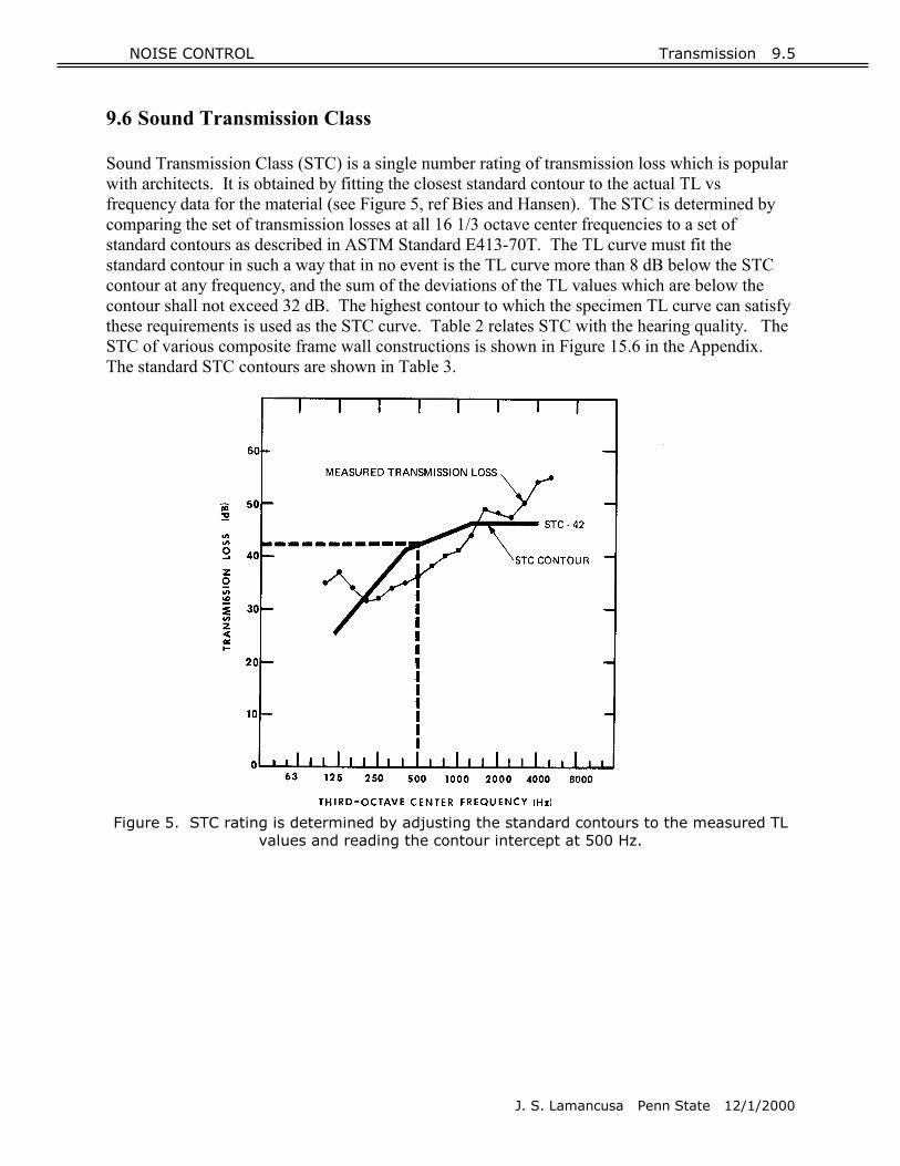
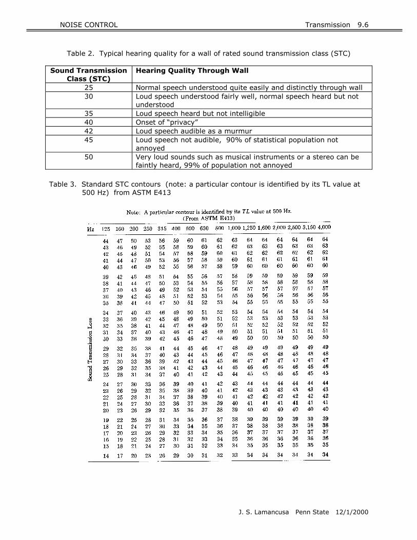
9.6 Sound Transmission Class Sound Transmission Class (STC) is a single number rating of transmission loss which is popular with architects. It is obtained by fitting the closest standard contour to the actual TL vs frequency data for the material (see Figure 5, ref Bies and Hansen). The STC is determined by comparing the set of transmission losses at all 16 1/3 octave center frequencies to a set of standard contours as described in ASTM Standard E413-70T. The TL curve must fit the standard contour in such a way that in no event is the TL curve more than 8 dB below the STC contour at any frequency, and the sum of the deviations of the TL values which are below the contour shall not exceed 32 dB. The highest contour to which the specimen TL curve can satisfy these requirements is used as the STC curve. Table 2 relates STC with the hearing quality. The STC of various composite frame wall constructions is shown in Figure 15.6 in the Appendix. The standard STC contours are shown in Table 3.

Figure 5. STC rating is determined by adjusting the standard contours to the measured TL

values and reading the contour intercept at 500 Hz.



Table 2. Typical hearing quality for a wall of rated sound transmission class (STC) Sound Transmission

Class (STC) Hearing Quality Through Wall

25 Normal speech understood quite easily and distinctly through wall 30 Loud speech understood fairly well, normal speech heard but not

understood 35 Loud speech heard but not intelligible 40 Onset of “privacy” 42 Loud speech audible as a murmur 45 Loud speech not audible, 90% of statistical population not

annoyed 50 Very loud sounds such as musical instruments or a stereo can be

faintly heard, 99% of population not annoyed Table 3. Standard STC contours (note: a particular contour is identified by its TL value at

500 Hz) from ASTM E413



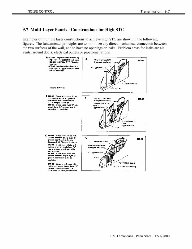
9.7 Multi-Layer Panels - Constructions for High STC Examples of multiple layer constructions to achieve high STC are shown in the following figures. The fundamental principles are to minimize any direct mechanical connection between the two surfaces of the wall, and to have no openings or leaks. Problem areas for leaks are air vents, around doors, electrical outlets or pipe penetrations.



Figure 6 Construction details of frame walls for high STC (courtesy of Owens Corning)

Similar considerations apply to floors and ceilings. Additionally, floors are rated by their Impact Insulation Class, (IIC). Resilient layers, or carpet are used to insulate the transmission of impact noise (such as footsteps). Layered floor constructions are shown in Figure 7.



Figure 7 Construction details for floor and ceiling systems that control impact sound (Courtesy of Owens Corning)



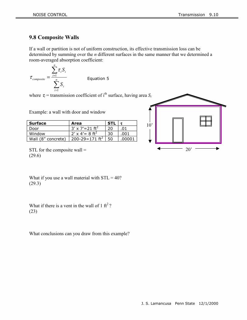
9.8 Composite Walls If a wall or partition is not of uniform construction, its effective transmission loss can be determined by summing over the n different surfaces in the same manner that we determined a room-averaged absorption coefficient:

�

�

=

== n

ii

i

n

ii

composite

S

S

1

1τ

τ Equation 5

where τi = transmission coefficient of ith surface, having area Si Example: a wall with door and window Surface Area STL ττττ Door 3’ x 7’=21 ft2 20 .01 Window 2’ x 4’= 8 ft2 30 .001 Wall (8” concrete) 200-29=171 ft2 50 .00001 STL for the composite wall = (29.6) What if you use a wall material with STL = 40? (29.3) What if there is a vent in the wall of 1 ft2 ? (23) What conclusions can you draw from this example?

20’

10’



9.9 Transmission Through Panels The transmission loss of an infinite homogeneous panel is shown in Figure 8.

Figure 8. Theoretical Transmission Loss for an infinite homogeneous panel STL or τ are highly dependent on frequency. The STL behavior can be divided into three basic regions. In Region I, at the lowest frequencies, the response is determined by the panel’s static stiffness. Depending on the internal damping in the panel, resonances can also occur which dramatically decrease the STL. Calculation of natural frequencies and modes shapes for panels is discussed in Section 9.9. In Region II (mass-controlled region), the response is dictated by the mass of the panel and the curve follows a 6dB/octave slope. Doubling the mass, or doubling the frequency, results in a 6 dB increase in transmission loss. In this region, the normal incidence transmission loss can be approximated by:

dB 2

1log102

0��

�

�

��

�

�

��

�

�+=

cTL S

ρωρ

Equation 6

where: ω = sound frequency (rad/sec) ρc =characteristic impedance of medium (415 rayls for air at standard temperature and

pressure) ρS =mass of panel per unit surface area The random incidence transmission loss is:

dB )23log(.10 00 TLTLTL −≈ Equation 7



In Region III, coincidence between the sound wavelength and the structural wavelength again decrease the STL. Coincidence is further described in Section 9.10. The actual behavior of some common building materials, shown in Figure 9, follows the same basic trends. It is most desirable to use a barrier material in its mass-controlled region.

10

20

30

40

50

60

70

63 125 250 500 1000 2000 4000 8000

Frequency - Hz

Tran

smis

sion

Los

s - d

B 9mm gypsumboard

12mm plywood

3mm lead

6mm glass

cinder block

Figure 9. Sound Transmission Loss of Typical Building Materials (data

from Table 8.1, Bies and Hansen) Properties which make for a good barrier material include: High density (gives high STL in mass-controlled region) Low bending stiffness (ideally want resonant frequencies below range of human hearing) High internal damping (prevents resonant modes from “ringing”) The ideal material for high STL is sheet lead, which has both high density and low stiffness. Unfortunately, due to environmental health concerns, lead can no longer be used. For the same reasons, gypsum board is a good barrier material and is more effective than plywood (which is stiffer and not as dense as gypsum board). Loaded vinyl, or vinyl impregnated with metal filings, is a common material for high STL.


9.10 Panel Natural Frequencies and Mode Shapes Knowledge of a panel’s natural frequencies and mode shapes is extremely helpful. It allows us to predict and hopefully avoid having excitation frequencies (harmonic forces generated by a machine) coincide with structural resonances. Knowledge of the mode shape is useful because: • provides guidance for stiffening a structure in order to change its natural frequencies; • provides guidance for adding laminated damping material to limit the response at resonance • the mode shape determines the radiation efficiency of the panel – if the structural

wavelength is larger than the acoustic wavelength, the panel will radiate very efficiently (discussed further in section 9.10)

Natural frequencies and mode shapes can be predicted by closed form solution of Euler’s thin plate approximation for some regular geometries including:

a) beams b) rectangular plates c) triangular plates d) circular plates e) rings

The natural frequencies of simply-supported, rectangular, thin, isotropic plate are described by a simple equation. Analytical solutions for other boundary conditions are not nearly so simple.

��

�

�

��

�

�

��

�

�

�+��

�

�

�=

222

122),(

y

y

x

xyx L

nLnEhnnf

ρπ Eq. 8

where: E = Young’s modulus h = plate thickness ρ = mass density/unit volume nx = x mode index, # of half sine waves along x axis ny = y mode index, # of half sine waves along y axis Lx = plate width in x direction Ly = plate width in y direction

The modeshape of the simply supported plate consists of

y

y

x

x

Lyn

LxnAyxz

ππsinsin),( = Equation 9

where z(x,y) is the transverse displacement at position (x, Example: Calculate the natural frequency of the 1,2

which is 0.125” thick. Material properties .283/386 lb sec2/in4

Answer: ��

��

�

�=22

2,1 301

)386/283(.12)125(.630

2ef π

x

Ly y

x

h

L

J. S. Lamancus

sinusoidal segm

y)

mode of a 30” for steel: E =

=��

��

�

�+2

302 63

z

a Penn State 12/1/2000

ents:

square steel plate 30e6 lb/in2 ρ =

.7 Hz



(1,1) 25.5 Hz (2,1) 63.7 Hz

(2,2) 101.9 Hz (1,3) 127.4 Hz

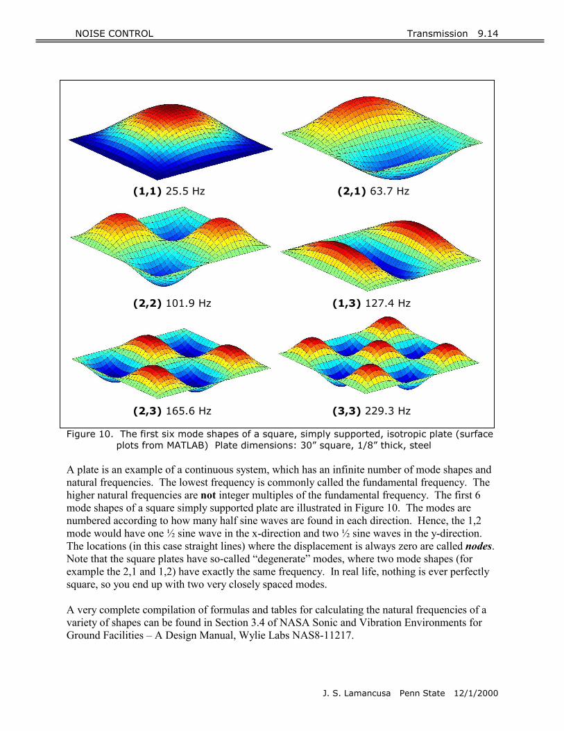
(2,3) 165.6 Hz (3,3) 229.3 Hz Figure 10. The first six mode shapes of a square, simply supported, isotropic plate (surface

plots from MATLAB) Plate dimensions: 30” square, 1/8” thick, steel A plate is an example of a continuous system, which has an infinite number of mode shapes and natural frequencies. The lowest frequency is commonly called the fundamental frequency. The higher natural frequencies are not integer multiples of the fundamental frequency. The first 6 mode shapes of a square simply supported plate are illustrated in Figure 10. The modes are numbered according to how many half sine waves are found in each direction. Hence, the 1,2 mode would have one ½ sine wave in the x-direction and two ½ sine waves in the y-direction. The locations (in this case straight lines) where the displacement is always zero are called nodes. Note that the square plates have so-called “degenerate” modes, where two mode shapes (for example the 2,1 and 1,2) have exactly the same frequency. In real life, nothing is ever perfectly square, so you end up with two very closely spaced modes. A very complete compilation of formulas and tables for calculating the natural frequencies of a variety of shapes can be found in Section 3.4 of NASA Sonic and Vibration Environments for Ground Facilities – A Design Manual, Wylie Labs NAS8-11217.



For complicated geometries, discretized numerical solutions, such as Finite Element Analysis (FEA) are commonly used. As an example, the ANSYS program was used to predict the frequencies and mode shapes of a clamped edge 24” x 30” x .125” plate. 80 thin plate elements were used. The predicted frequencies are compared to experimental data, and to the analytical solution (using the NASA tables), in Table 3. Note that FEA solutions typically over-predict the natural frequencies. The agreement improves if more elements are used to discretize the structure. Table 3. Comparison of experimental, FEA (ANSYS program), and analytical results for a 30” x 24” x .125” steel plate with clamped edges

Mode 1,1 2,1 1,2 3,1 Experimental Natural Freq - Hz 62.5 95 125 160 FEA - Hz 64.5 112 148 190 Analytical - Hz 63 111 144 188

Experimental methods to find natural frequencies and mode shapes include modal analysis, where a known input force is applied by a shaker, or an impact, and the frequency response is measured using FFT techniques. Mode shapes can also be determined visually by an antique, but clever technique - Chladni patterns. In this method, sand spread on a plate, which is vibrating at resonance, collects at the nodal lines (see Figure 11).

Figure 11. Chladni patterns for violin top and back plates (Cover of Scientific

American Magazine, October 1981)



9.11 Coincidence Effects Getting back to Region III of Figure 6, we see a pronounced dip in the transmission loss curve. This occurs when the wavelength of sound in air coincides with the structural wavelength. At this frequency (and above), efficient radiation of sound occurs. For a homogeneous, infinite plate, this “critical frequency” is:

Hz 102.5Eh

efcρ= Equation 10

where: ρ = weight density (lb/in3) h = plate thickness (inches) E = elastic modulus (psi)

For glass, steel or aluminum (all have similar ρ/E), this simplifies to: h

fc500≈

For plywoodh

fc790≈ . Drywall typically exhibits a 5-10 dB dip in TL at ~500 Hz.

The ideal barrier material has high density and low bending stiffness (i.e. very limp). In the old days, lead sheet or leaded vinyl were widely used. Today, loaded vinyl (impregnated with non-lead metal) is a good choice. Dense, limp materials tend to push the coincidence frequency upward and out of the range of interest. Coincidence dips are a problem for materials with low internal damping and high bending stiffness (such as metals or glass). The radiation efficiency of a simply supported square plate in the vicinity of coincidence is shown in Figure 10 (ref. Wallace, 1972).

Figure 12. Radiation efficiency for modes of a simply supported square panel

1.0

10-1

10-2 Radiation Efficiency σ

10-3

10-4

k/kb



Radiation efficiency, σ is defined as the ratio of the actual energy radiated (W) by the structure to the amount of energy that would be radiated by a circular piston of the same area (S) and having the same mean square normal velocity <VN

2>, and having a diameter much larger than the wavelength in air:

2

21

NVcS

W

ρσ = Equation 11

The horizontal axis of Figure 12, k/kb, is the ratio between structural and acoustic wave numbers (ratio of structural wavelength to the acoustic wavelength). The plate dimensions are a,b and n,m are the number of ½ sine waves in each plate dimension.

plateb

air bm

ankck

λπππ

λπω 2 2/

22

=��

��

�+��

��

�=== Equation 12

All modes become very efficient radiators near coincidence. Below coincidence, some radiation still occurs, predominantly from the corners and edges of the plate as shown in Figure 13. Adjacent peaks and valleys on the surface cancel each other, leaving just the edges to radiate. The odd modes (such as 1,1 1,3 …) radiate better that the even modes (2,2 2,4 …) because the uncancelled portions are in phase with each other (two monopoles).

Figure 13. Local cancellation on vibrating plates below coincidence, top) odd mode – uncancelled segments are in phase – two monopoles; bottom) even mode – uncancelled segments are out of phase, forming a dipole

which is not as efficient a radiator as two monopoles



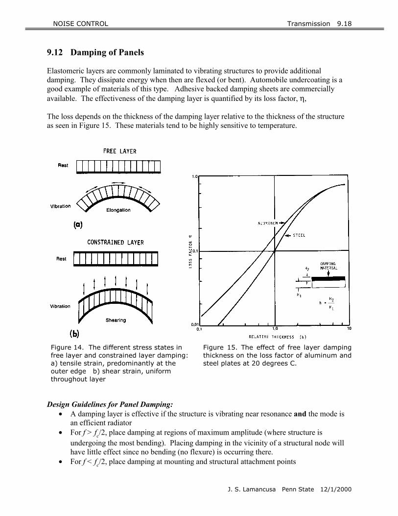
9.12 Damping of Panels Elastomeric layers are commonly laminated to vibrating structures to provide additional damping. They dissipate energy when then are flexed (or bent). Automobile undercoating is a good example of materials of this type. Adhesive backed damping sheets are commercially available. The effectiveness of the damping layer is quantified by its loss factor, η, The loss depends on the thickness of the damping layer relative to the thickness of the structure as seen in Figure 15. These materials tend to be highly sensitive to temperature.

Figure 14. The different stress states in free layer and constrained layer damping: a) tensile strain, predominantly at the outer edge b) shear strain, uniform throughout layer

Figure 15. The effect of free layer damping thickness on the loss factor of aluminum and steel plates at 20 degrees C.

Design Guidelines for Panel Damping:

• A damping layer is effective if the structure is vibrating near resonance and the mode is an efficient radiator

• For f > fc/2, place damping at regions of maximum amplitude (where structure is undergoing the most bending). Placing damping in the vicinity of a structural node will have little effect since no bending (no flexure) is occurring there.

• For f < fc/2, place damping at mounting and structural attachment points



• Cover 40% of structural wavelength – free layer damping • Cover 60% of structural wavelength – constrained layer damping • Free layer guidelines:

A thin layer, ½ t or 10% of weight will eliminate the “ring” Use 2 to 3 times the thickness of the structure to achieve loss factor η from .3-.6

9. TRANSMISSION OF SOUND THROUGH STRUCTURES

Documents

Transcript of 9. TRANSMISSION OF SOUND THROUGH STRUCTURES