3D Reconstruction from Two 2D Images Ted Shultz and...

Shultz, Rodriguez, ECE 533 Fall 2003 of 14

3D Reconstruction from Two 2D Images Ted Shultz and Luis A. Rodriguez

Abstract A Matlab algorithm was developed to partially reconstruct a real scene using two static images taken of the scene with an un-calibrated camera. The algorithm displays the two images and the user matches corresponding points in both images. From the displacement of the selected image points the algorithm estimates a depth surface for the scene. The original image is then” draped” over the depth surface to create a depth field on the image. The reconstructed scene with depth perception is then rotated and the frames are saved to create a movie showing the different views of the scene. Introduction Often times only 2-D representations of our 3-D world exists. For instance, satellite images taken of remote places (Mount Everest) and/or harsh environments (war zone) where it would hazardous or dangerous for human’s presence but where it would advantageous to have knowledge of the spatial conditions of the environment of interest. Images of a scene provide very valuable information, but they simply lack the spatial information that we are accustomed to for navigating around our environment. A partial reconstruction of the scene will prove useful in providing a better visualization of that scene for closely scrutinizing the environment and as a result give the user a sense of “presence” without actually ever being in the scene. Previous work for the reconstruction of a real world scene from images is heavily based on projective and epipolar geometry [1]. The common approach is to find the relationship between the different images by calculating their fundamental matrixes, which expresses the image’s incidence relation. These matrixes in addition to a simple pinhole camera model can then be used to find the correspondence between points. A novel view can then be found from the intersection of the epipolar lines of the other two views. In this project report we propose a different methodology for a similar 3D reconstruction result to the projective geometry approach, which is less computationally expensive and less mathematically convoluted. Approach The general approach used for this project was to: Acquire digital images, match up key points in both images, estimate a depth mask, and finally generate an image from a new view. This approach was used for two scenes presented in this report. Captured Images The algorithm we developed uses two images of the same scene. To get these images a digital camera was used. For one set of our images (the cluttered room) the camera


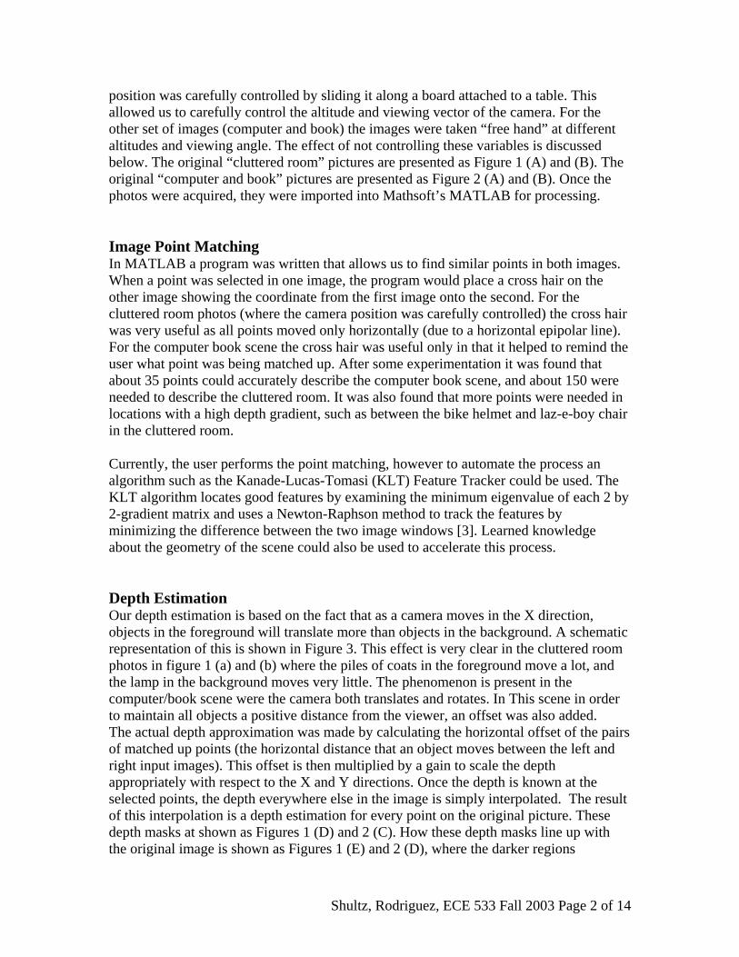
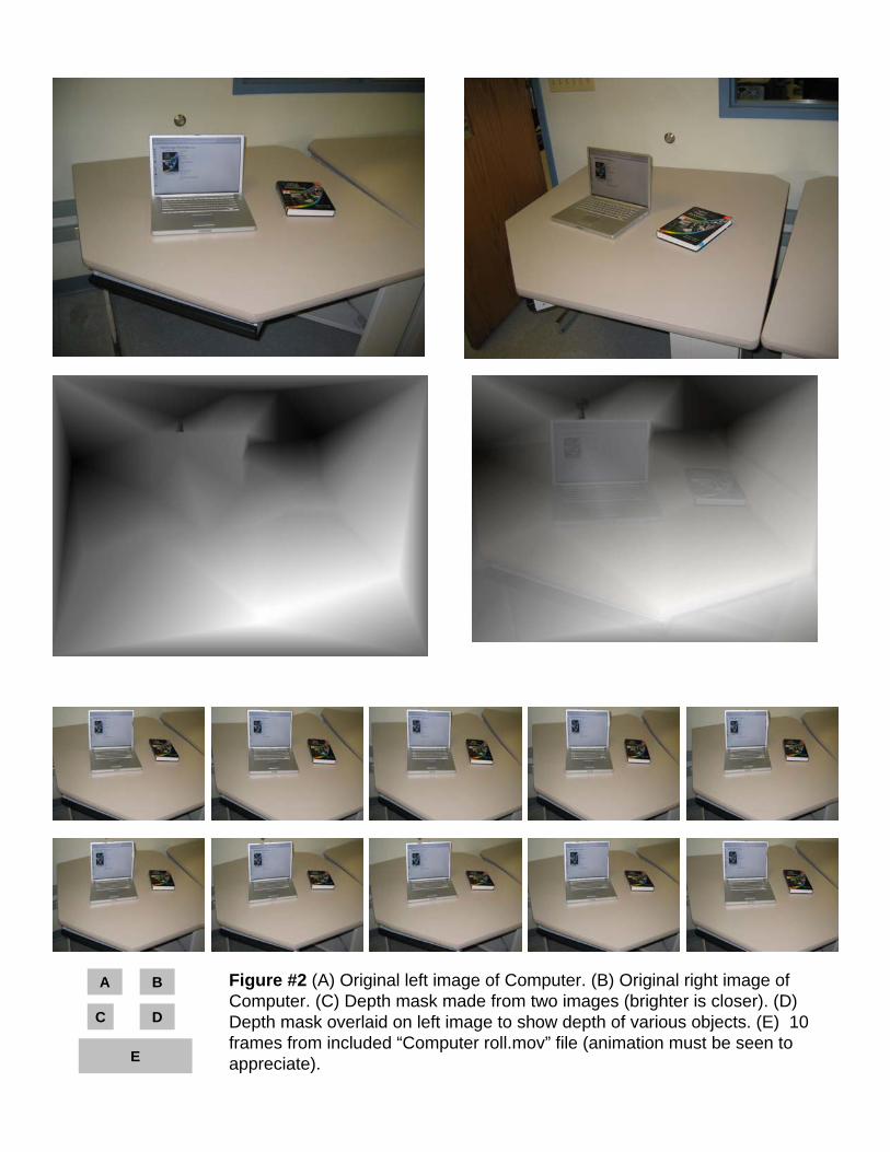
position was carefully controlled by sliding it along a board attached to a table. This allowed us to carefully control the altitude and viewing vector of the camera. For the other set of images (computer and book) the images were taken “free hand” at different altitudes and viewing angle. The effect of not controlling these variables is discussed below. The original “cluttered room” pictures are presented as Figure 1 (A) and (B). The original “computer and book” pictures are presented as Figure 2 (A) and (B). Once the photos were acquired, they were imported into Mathsoft’s MATLAB for processing. Image Point Matching In MATLAB a program was written that allows us to find similar points in both images. When a point was selected in one image, the program would place a cross hair on the other image showing the coordinate from the first image onto the second. For the cluttered room photos (where the camera position was carefully controlled) the cross hair was very useful as all points moved only horizontally (due to a horizontal epipolar line). For the computer book scene the cross hair was useful only in that it helped to remind the user what point was being matched up. After some experimentation it was found that about 35 points could accurately describe the computer book scene, and about 150 were needed to describe the cluttered room. It was also found that more points were needed in locations with a high depth gradient, such as between the bike helmet and laz-e-boy chair in the cluttered room. Currently, the user performs the point matching, however to automate the process an algorithm such as the Kanade-Lucas-Tomasi (KLT) Feature Tracker could be used. The KLT algorithm locates good features by examining the minimum eigenvalue of each 2 by 2-gradient matrix and uses a Newton-Raphson method to track the features by minimizing the difference between the two image windows [3]. Learned knowledge about the geometry of the scene could also be used to accelerate this process. Depth Estimation Our depth estimation is based on the fact that as a camera moves in the X direction, objects in the foreground will translate more than objects in the background. A schematic representation of this is shown in Figure 3. This effect is very clear in the cluttered room photos in figure 1 (a) and (b) where the piles of coats in the foreground move a lot, and the lamp in the background moves very little. The phenomenon is present in the computer/book scene were the camera both translates and rotates. In This scene in order to maintain all objects a positive distance from the viewer, an offset was also added. The actual depth approximation was made by calculating the horizontal offset of the pairs of matched up points (the horizontal distance that an object moves between the left and right input images). This offset is then multiplied by a gain to scale the depth appropriately with respect to the X and Y directions. Once the depth is known at the selected points, the depth everywhere else in the image is simply interpolated. The result of this interpolation is a depth estimation for every point on the original picture. These depth masks at shown as Figures 1 (D) and 2 (C). How these depth masks line up with the original image is shown as Figures 1 (E) and 2 (D), where the darker regions

A B

DC

E

F

Figure #1 (A) Original left image of room. (B) Original right image of room. (C) Left image with dots showing 150 locations that were found in both images. (D) Depth mask made from two images (brighter is closer). (E) Depth mask overlaid on left image to show depth of various objects. (F) 10 frames from included “Room Slide.mov” file.

A B

C

E

D

Figure #2 (A) Original left image of Computer. (B) Original right image of Computer. (C) Depth mask made from two images (brighter is closer). (D) Depth mask overlaid on left image to show depth of various objects. (E) 10 frames from included “Computer roll.mov” file (animation must be seen to appreciate).


represent that the object is far away and lighter regions represent the object is closer to the user. Simulating a 3D image Once the 3D mask exists, we created a new surface in MATLAB with this 3D data, and used one of the original images as a texture to be placed over this surface. This technique allows us to then move the camera position and estimate different views that were not photographed! By moving the camera along a path by our simulated 3D environment, we were able to create short movies that appear as if there were taken by a video camera moving around in the 3D environment! These impressive videos are included on the CD that accompanies this report.

Figure 3

Left Image Right Image

Camera Camera


Work Performed Several programs were written in order to complete this project. They include: FindPoints.m – This is the program that is used to find similar points in two images. It is included at the end of this report at Appendix A as well as in the appendix folder on the CD. Slide.m – This is the program that is used to make a 3D surface and have the camera move horizontally in front of it. It is included at the end of this report at Appendix B as well as in the appendix folder on the CD. Roll.m – This is the program that is used to make a 3D surface and have the camera move in a circular fassion in front of it. It is included at the end of this report at Appendix C as well as in the appendix folder on the CD. Frams2ims.m – This is the program that is used to make a series of numbered images from a movie file in MATLAB. This program was written so that the moves could be exported and included on the CD. It is included at the end of this report at Appendix D as well as in the appendix folder on the CD. Also included on the CD, but not feasible for the written report are the generated videos. Results Two scenes were reconstructed using two static images of each scene. The first scene was that of a cluttered room and the second scene was that of a computer and a book on a table. For the cluttered room two video clips were produced, one shows the room scanned from right to left and the second shows the room scanned in circular manner. All video clips are included in the provided CD. For the scene of the computer and the book one clip was produced that shows a roll motion of the image. All three video clips give a sense of depth in the image. The combination of the image “draped” on the estimated depth surface of the scene and the creation of frames by slowly viewing the depth enhanced image surface gives the eye a false perception of depth. During the reconstruction of the 3D scene we encountered instances where distortion between reconstructed frames was prevalent. This problem was caused by the occlusion of features in one image that were present in the second, in this case no corresponding image points could be chosen. Distortion was also observed where a feature was represented by a smaller number of pixels in one image than in the other image so that there was no one-to-one correspondence. To partially alleviate this problem more corresponding points were chosen around the area of the feature where less pixel information was available. If an actual estimation of the depth is necessary instead of just the perception field effect as done here for this project, some calibration is necessary. For instance, a depth of X number of pixels is equivalent to Y number of feet.


An advantage of this algorithm is that if a quick 3D reconstruction is desired not much computational is necessary and the depth accuracy of the reconstructed scene can be tremendously improved simply by selecting more corresponding image points. No camera calibration is necessary and no intrinsic or extrinsic camera parameters need to be determined. Future work to enhance or build on this project include implementing a KLT feature tracking algorithm to make the selection of corresponding image points less tedious for the user. Secondly, modifying this algorithm so that more than two images can be used for reconstructing the scene, could also result in dramatically improved images. Reference: [1] Theo Moons, A Guided Tour Through Multiview Relations, (2000) Katholieke

Universiteit Leuven, ESAT/ PSI, Kardinaal Mercierlaan 94,3001 Leuven, Belgium. [2] Waack, Fritz G, An Introduction to Stereo Photo technology and practical suggestions

for Stereo Photography, 1985. [3] Jianbo Shi and Carlo Tomasi. Good Features to Track. IEEE Conference on

Computer Vision and Pattern Recognition, pages 593-600, 1994


Appendix A Code for findpoints.m % find points disp (' This Program was written by Ted Shultz and Luis Rodriguez') disp (' as a final project for ECE 533.') disp (' ') % get the name of the file for the left image. left_name = input('Enter the name of the left image (default is room0008.jpg): ','s'); if isempty(left_name) left_name = 'room0008.jpg'; end % get the name of the file for the right image. right_name = input('Enter the name of the left image (default is room0010.jpg): ','s'); if isempty(right_name) right_name = 'room0010.jpg'; end % get the name of the file for the right image. num_point = input('Enter the number of common points to find (default is 15): '); if isempty(num_point) num_point = 15; end % get the name of the file for the right image. depth_ex = input('Enter the depth exaggeration (default is 5): '); if isempty(depth_ex) depth_ex = 5; end % now load the images of the file names just gotten left = imread(left_name); right = imread(right_name); % a copy of the right image is also made because the right image will have % lines added to it, and so it will be nessesary to keep a copy trueright=right; trueleft = left; % set up the figure window without menubar and such fig = figure; imshow(left); title('left image') %set(fig,'Selected','on','visible','on') set(fig,'Selected','on','menubar','none','visible','on') % thise are two arrays that keep track of all the inputs as given by the


% user left_points = zeros(num_point,2); right_points = zeros(num_point,2); disp (' ') disp ('Find the same point in both the left and right views') disp (' ') % loop for the number of points to find for i=1:num_point % show the left image, and have the user click on a point imshow(left) title('left image') left_points(i,:)=ginput(1); % Add a red square in location of points already done on left side left ((floor(left_points(i,2))-1):(ceil(left_points(i,2))+1),(floor(left_points(i,1))-1):(ceil(left_points(i,1))+1),2:3)=0; %left_points(i,:) % add RED hoizonal lines to right side right (floor(left_points(i,2))-1,:,2:3)=0; right (ceil(left_points(i,2))+1,:,2:3)=0; % add RED vertical lines to right side right (:,floor(left_points(i,1))-1,2:3)=0; right (:,ceil(left_points(i,1))+1,2:3)=0; % get the points that the user clicked on imshow(right) title('right image') right_points(i,:)=ginput(1); % revert image back to original (without cross hairs) right=trueright; end disp (' ') disp ('Done finding points, run roll or slide to make 3D') disp (' ')


Appendix B Code for roll.m disp (' ') disp ('Now calculating frams of movie') disp (' ') fig = figure; %roll % set up the figure without any title stuff so that movie looks good set(fig,'Selected','off','menubar','none','visible','on') title('') % calculate points for depth field, % the location is equal to the location in the left frame (master image) % the depth is equal to the the horizontal distance between the left and % right frame. left_depth = [left_points(:,2),left_points(:,1),(left_points(:,1)-right_points(:,1))]; %left_points %right_points [m,n,trash] = size(left); % m is height (480 for default), n is width (680 for default ) of image % image cord is hight by width % make a meshgrid of the same size of the original image. this will allow % us to interpret all the points for a depth field [XI,YI] = meshgrid(1:n,1:m); % this matrix is in the form, down, over, depth % now we'll add depths of zero to the four corners % this will help keep the image looking normal left_depth=[left_depth;0,0,0;0,n,0;m,0,0;m,n,0]; % this next part is used to interpalate all the depths points for the % entire meshgrid. the depth_ex is used to set the level of exaggeration ZI = griddata(left_depth(:,2),left_depth(:,1),left_depth(:,3)*depth_ex,XI,YI); % this next part is used to "drape" our image over the depth field surface(ZI,trueleft,... 'FaceColor','texturemap',... 'EdgeColor','none',... 'CDataMapping','direct')


% the rest of this is just setting the camera position to make it all look % good set(gca,'CameraTargetMode','manual') cam_dist=10000; rad = 700; % Record the movie for j = 1:20 % make the camera spin campos([320+1.2*rad*cos(pi*j/10),240+.7*rad*sin(pi*j/10),-1*cam_dist]) set(gca,'CameraUpVector',[0 -1 0],'CameraTarget',[320,240,0],'CameraViewAngle',3) F(j) = getframe(gcf); end disp (' ') disp ('Now showing frams of movie') disp (' ') movie(F,5) disp (' ') disp ('done with movie, to export as a file, run "frames2ims" ') disp (' ')


Appendix C Code for slide.m % Slide disp (' ') disp ('Now calculating frams of movie') disp (' ') % set up the figure without any title stuff so that movie looks good fig = figure; set(fig,'Selected','off','menubar','none','visible','on') title('') % calculate points for depth field, % the location is equal to the location in the left frame (master image) % the depth is equal to the the horizontal distance between the left and % right frame. left_depth = [left_points(:,2),left_points(:,1),(left_points(:,1)-right_points(:,1))]; %left_points %right_points [m,n,trash] = size(left); % m is height (480 for default), n is width (680 for default ) of image % image cord is hight by width % make a meshgrid of the same size of the original image. this will allow % us to interpret all the points for a depth field [XI,YI] = meshgrid(1:n,1:m); % this matrix is in the form, down, over, depth % now we'll add depths of zero to the four corners % this will help keep the image looking normal left_depth=[left_depth;0,0,0;0,n,0;m,0,0;m,n,0]; % this next part is used to interpalate all the depths points for the % entire meshgrid. the depth_ex is used to set the level of exaggeration ZI = griddata(left_depth(:,2),left_depth(:,1),left_depth(:,3)*depth_ex,XI,YI); % this next part is used to "drape" our image over the depth field surface(ZI,trueleft,... 'FaceColor','texturemap',... 'EdgeColor','none',... 'CDataMapping','direct') % the rest of this is just setting the camera position to make it all look


% good set(gca,'CameraTargetMode','manual') cam_dist=5000; % Record the movie for j = 1:20 campos([320+sin((j/2-5)*pi/180)*cam_dist,240,-1*cos((j/2-5)*pi/180)*cam_dist]) set(gca,'CameraUpVector',[0 -1 0],'CameraTarget',[320,240,0],'CameraViewAngle',5.5) F(j) = getframe(gcf); end disp (' ') disp ('Now showing frams of movie') disp (' ') movie(F,5) disp (' ') disp ('done with movie, to export as a file, run "frames2ims" ') disp (' ')


Appendix D Code for frames2ims.m function frames2ims(rootName,format,F) %rootName : root name of the frames %Formats %'jpg'or 'jpeg','bmp','tif','hdf','pbm','png',pnm' %F structure containting the frames mkdir MOVIE; %make directory to store Movie frames; [junk,numFrames] = size(F); for i = 1:numFrames frame = frame2im(F(i)); imname = strcat(rootName, num2str(i,'%04.0f'),'.',format); cd MOVIE imwrite(frame,imname,format) cd .. end

3D Reconstruction from Two 2D Images Ted Shultz and...

Documents

Transcript of 3D Reconstruction from Two 2D Images Ted Shultz and...