remote sensing

Article

A Methodology for the Reconstruction of 2DHorizontal Wind Fields of Wind Turbine WakesBased on Dual-Doppler Lidar Measurements

Marijn F. van Dooren *, Davide Trabucchi and Martin Kühn

ForWind, University of Oldenburg, Küpkersweg 70, 26129 Oldenburg, Germany;davide.trabucchi@uni-oldenburg.de (D.T.); martin.kuehn@uni-oldenburg.de (M.K.)* Correspondence: marijn.vandooren@uni-oldenburg.de; Tel.: +49-441-798-5064

Academic Editors: Charlotte Bay Hasager, Alfredo Peña Diaz, Xiaofeng Li and Prasad S. ThenkabailReceived: 11 May 2016; Accepted: 22 September 2016; Published: 29 September 2016

Abstract: Dual-Doppler lidar is a powerful remote sensing technique that can accurately measurehorizontal wind speeds and enable the reconstruction of two-dimensional wind fields based onmeasurements from two separate lidars. Previous research has provided a framework of dual-Doppleralgorithms for processing both radar and lidar measurements, but their application to wakemeasurements has not been addressed in detail yet. The objective of this paper is to reconstructtwo-dimensional wind fields of wind turbine wakes and assess the performance of dual-Doppler lidarscanning strategies, using the newly developed Multiple-Lidar Wind Field Evaluation Algorithm(MuLiWEA). This processes non-synchronous dual-Doppler lidar measurements and solves thehorizontal wind field with a set of linear equations, also considering the mass continuity equation.MuLiWEA was applied on simulated measurements of a simulated wind turbine wake, with twotypical dual-Doppler lidar measurement scenarios. The results showed inaccuracies caused by theinhomogeneous spatial distribution of the measurements in all directions, related to the ground-basedscanning of a wind field at wind turbine hub height. Additionally, MuLiWEA was applied on areal dual-Doppler lidar measurement scenario in the German offshore wind farm “alpha ventus”.It was concluded that the performance of both simulated and real lidar measurement scenariosin combination with MuLiWEA is promising. Although the accuracy of the reconstructed windfields is compromised by the practical limitations of an offshore dual-Doppler lidar measurementsetup, the performance shows sufficient accuracy to serve as a basis for 10 min average steady wakemodel validation.

Keywords: long-range scanning lidar; plan position indicator (PPI); wind field reconstruction;wake measurement

1. Introduction

Establishing sophisticated methods for measurement and analysis of wake effects [1] in windfarms is relevant nowadays, since large offshore wind farms can experience wake losses of between10% and 20% of their annual energy production [2]. By acquiring more knowledge about wakes,their negative impacts on large wind farms can be mitigated e.g., by improving wind farm layoutdesign [3] or by applying innovative wind farm control strategies [4].

The high potential of lidars [5,6] has been demonstrated for different wind energy applications ingeneral [7–9], and for measuring wakes in particular [10,11]. Coherent Doppler lidars [12,13] measurethe Doppler shift of frequency between the emitted and backscattered laser light, which is convertedto a radial velocity estimate. Long-range pulsed lidars [14] offer the possibility to scan over areas ofseveral square kilometers within a few minutes. Käsler et al. [15] were among the first to execute wake

Remote Sens. 2016, 8, 809; doi:10.3390/rs8100809 www.mdpi.com/journal/remotesensing

Remote Sens. 2016, 8, 809 2 of 15

measurements of a turbine with such a lidar. Aitken et al. [16] retrieved wake characteristics by usingone long-range lidar and fitting measurements to Gaussian-shaped wake profiles. Banta et al. [17]proposed a way to execute volumetric measurements with a single lidar. Iungo et al. [18] useddual-Doppler lidar to scan a vertical plane through a wind turbine wake.

Considerable uncertainties can affect the horizontal wind vector reconstructed from measurementsperformed with a single lidar. This aspect is even more relevant in the wake of a wind turbine where thewind field is heterogeneous. Using a single representative wind direction—e.g., provided by a nearbywind vane—to evaluate the horizontal wind vector derived from the radial wind velocity measuredover a large area within a wind farm, could introduce uncertainties due to the local variability ofthe wind direction. Moreover, the propagation of all uncertainties affecting the reconstruction of thehorizontal wind vector tends to grow infinitely when the lidar measures perpendicular to the winddirection. This limits the possibility to perform reliable measurements of a wind turbine wake.

Advanced dual-Doppler lidar applications could overcome these problems by using multiplelidars to scan over the same area of interest from different locations, optionally considering thecontinuity equation as well. We are subsequently referring to dual-Doppler lidar as methods forperforming and processing measurements from different Plan Position Indicator (PPI) scans oftwo long-range pulsed scanning lidars. The PPI scan is characterised by a fixed elevation angleand a varying azimuth angle. When several elevation angles are considered and a full-volume ofdual-Doppler lidar measurements is available, it is possible to evaluate 2D or 3D wind fields ona predefined grid by means of algorithms such as the Multiple-Doppler Synthesis and ContinuityAdjustment Technique (MUSCAT) by [19]. This was originally developed for airborne radar [20] andwas evaluated mainly for the study of meteorological steady wind fields in which the measurementdomain was in the order of 1000 km2 [21]. Drechsel et al. [22] demonstrated the feasibility of theapplication of MUSCAT to ground-based dual-Doppler lidar measurements. In the latter study,a full-volume scan defined by a 360◦ sector at 10 different elevation angles lasted about 20 min.This points out that the small time and length scale dynamics of wind turbine wakes and thetime needed for a full-volume scan cycle could conflict when applying dual-Doppler lidar to wakemeasurements. On the contrary, with a full-volume scan cycle of about 1 min, the application oftwo Ka-band radars [23] could enable the study of the dynamical behaviour of wakes in a wind farm.

Although the application of the aforementioned dual-Doppler analysis algorithms in combinationwith the state-of-the-art dual-Doppler lidar scanning techniques was demonstrated before,the application to wind turbine wakes has not been analysed thoroughly yet. In this paper, we proposea simple wind field reconstruction methodology similar to MUSCAT, which we call Multiple-LidarWind Field Evaluation Algorithm (MuLiWEA). This implementation is meant to reduce the uncertaintyin the evaluation of the horizontal wind speeds, especially for situations in which the inclinationbetween the wind direction and the line-of-sight direction of the radial wind speed measurement ofone lidar is close to 90◦.

The application of MuLiWEA does not require a set of fully synchronised dual-Doppler lidarmeasurements because it performs grid interpolation. This feature offers the possibility to usemeasurements from scanning scenarios with low complexity and fast area coverage.

We applied MuLiWEA to dual-Doppler lidar measurements simulated in the wake of a windturbine, considering a series of different scanning scenarios, and compared the reconstructed windfields to the simulated ones. Additionally, we analysed a test case based on real dual-Doppler lidarmeasurements offshore.

2. Methodology

The MuLiWEA algorithm is based on the following assumptions:

• The vertical wind speed component w is neglected because the elevation angles of the PPI scansare commonly small, and, therefore, it is difficult to estimate this component accurately from themeasured line-of-sight velocity. This assumption limits the application of MuLiWEA to horizontal

Remote Sens. 2016, 8, 809 3 of 15

flows only, i.e., it might not be accurate in complex terrain sites, in convective atmosphereconditions, or in the near wake of a wind turbine.

• As a consequence of the previous assumption, no vertical transport of mass is considered in thecontinuity equation, which is therefore applied in its two-dimensional form.

• The flow is assumed to be stationary for the required time resolution because it generally takes afew minutes for the lidar scans to cover an area of interest, and it is useful to average a number ofsubsequent PPI scans to improve the data quality.

• The flow is assumed to be incompressible.

The measured line-of-sight velocity vLOS is expressed in the Cartesian wind speed components inthe x- and y-direction, namely u and v, respectively, by Equation (1):

αku + βkv = vLOSk , (1)

with α = sin(χ) cos(δ) and β = cos(χ) cos(δ).Note that Equation (1) already incorporates that w = 0. The line-of-sight direction at a single

measurement point k is defined by the azimuth angle χ and elevation angle δ of a lidar scanning beam(see Figure 1). The azimuth angle is expressed in the geographical reference system, i.e., χ = 0◦ isdirected to the North and increases clockwise. Since the angles are a known input with a certainpointing accuracy, the two remaining unknowns in Equation (1) are u and v. To solve for these two windspeed components, at least two linearly independent vLOS measurements are needed. Instead of fullysynchronised measurements of two lidars at a single point in space at the same time (e.g., [18]),a concept to reconstruct 2D wind vector information from a larger set of PPI measurements fromtwo lidars is used. In the worst case, the measurements are neither synchronised in time nor space.Therefore, the method has to analyse samples of K measurements from the two lidars around each gridpoint p (see Figure 2) over a longer time period of e.g., ten minutes. Measurements in the near vicinityof a grid point rather than exactly at a grid point have to be used and measurements at different heightsabove ground have to be combined. A suitable protocol for measurement point selection is found inthe form of the Quad-Doppler wind synthesis, a step of the Extended Overdetermined dual-DopplerFormalism (EODD) [20], later also used by Newsom et al. [24]. The reconstruction of a wind field canbe divided into five sequential steps:

1. A temporal and spatial domain is defined. To ensure that an area of interest is covered with atleast one PPI scan per lidar, and possibly multiple overlapping scans to enhance averaging, a timeresolution of ten minutes is chosen. A Cartesian grid is generated on the area of interest coveredby the overlapping PPI scans. The assumption of stationarity posed before is considered to bereasonable for this time scale.

2. For each grid point p, the measurement set K that is located within its surrounding circle withradius R, i.e., the radius of influence, is used to compute the local wind vector. The measurementset K contains contributions from all lidars (see Figure 2). Different lidars do not necessarily haveto contribute an equal number of measurements for the same grid point.

3. For each grid point p, a linear system based on Equation (1) can be established , which considersall measurements k = 1, ..., K per circle with radius R [20]:[

∑Kk=1(α

2kwk) ∑K

k=1(αkβkwk)

∑Kk=1(αkβkwk) ∑K

k=1(β2kwk)

]p

[uv

]p

=

[∑K

k=1(αkwkvLOSk )

∑Kk=1(βkwkvLOSk )

]p,

(2)

Remote Sens. 2016, 8, 809 4 of 15

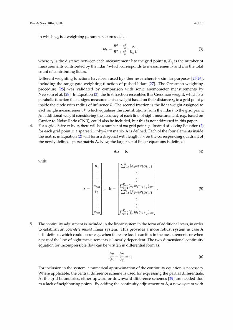
in which wk is a weighting parameter, expressed as:

wk =R2 − r2

kR2 + r2

k· K

Klk L, (3)

where rk is the distance between each measurement k to the grid point p, Klk is the number ofmeasurements contributed by the lidar l which corresponds to measurement k and L is the totalcount of contributing lidars.

Different weighting functions have been used by other researchers for similar purposes [25,26],including the range gate weighting function of pulsed lidars [27]. The Cressman weightingprocedure [25] was validated by comparison with sonic anemometer measurements byNewsom et al. [28]. In Equation (3), the first fraction resembles this Cressman weight, which is aparabolic function that assigns measurements a weight based on their distance rk to a grid point pinside the circle with radius of influence R. The second fraction is the lidar weight assigned toeach single measurement k, which equalises the contributions from the lidars to the grid point.An additional weight considering the accuracy of each line-of-sight measurement, e.g., based onCarrier-to-Noise-Ratio (CNR), could also be included, but this is not addressed in this paper.

4. For a grid of size m-by-n, there will be a number of mn grid points p. Instead of solving Equation (2)for each grid point p, a sparse 2mn-by-2mn matrix A is defined. Each of the four elements insidethe matrix in Equation (2) will form a diagonal with length mn on the corresponding quadrant ofthe newly defined sparse matrix A. Now, the larger set of linear equations is defined:

A x = b, (4)

with:

x =

u1......

umn

v1......

vmn

, b =

∑K1k=1(αkwkvLOSk )1

...

...∑Kmn

k=1(αkwkvLOSk )mn

∑K1k=1(βkwkvLOSk )1

...

...∑Kmn

k=1(βkwkvLOSk )mn

. (5)

5. The continuity adjustment is included in the linear system in the form of additional rows, in orderto establish an over-determined linear system. This provides a more robust system in case Ais ill-defined, which could occur e.g., when there are local scarcities in the measurements or whena part of the line-of-sight measurements is linearly dependent. The two-dimensional continuityequation for incompressible flow can be written in differential form as:

∂u∂x

+∂v∂y

= 0. (6)

For inclusion in the system, a numerical approximation of the continuity equation is necessary.Where applicable, the central difference scheme is used for expressing the partial differentials.At the grid boundaries, either upward or downward difference schemes [29] are needed dueto a lack of neighboring points. By adding the continuity adjustment to A, a new system with

Remote Sens. 2016, 8, 809 5 of 15

the 3mn-by-2mn matrix AC is created. There are still 2mn unknown variables, leaving the vectorx unaffected. The vector bC is generated by extending b with mn zeros. The final linear system,

AC x = bC, (7)

is an over-determined linear system, which is solved by minimising its squared residuals.

05

1

z [k

m]

2

4 5

δχ

3 4

y [km], N, 0°

3

x [km], E, 90°

221 1

0 0

Figure 1. Illustration of a plan position indicator (PPI) scan with the azimuth angle χ and elevationangle δ indicated.

Figure 2. Schematic view of a Cartesian grid with indicated measurement positions of two lidars in thevicinity with radius R of a grid point p.

3. Application and Validation of MuLiWEA

3.1. Simulated Dual-Doppler Lidar Measurement Scenarios

To test MuLiWEA, different lidar measurement scenarios were simulated considering a weightedaverage of the line-of-sight velocity over the considered sample volume. The sample volume wasdefined along a linear coordinate s, which represents the line-of-sight distance from the lidar to thetarget point. We used a range gate length corresponding to a spatial extension ∆p of 36 m and aGaussian laser pulse with intensity Ip, characterised by a Full Width Half Maximum ∆r of 30 m [14]:

Ip(s) =1√π∆r

e(− s2

∆r2

). (8)

Remote Sens. 2016, 8, 809 6 of 15

The estimated line-of-sight velocity is then v̂LOS(s) = 1∆p∫ ∆p

2

−∆p2

vp (s) ds, where vp(s) =

∫ kp ∆r2

−kp ∆r2

vr′ (s′ − s) I (s′ − s) ds′ with I = Ip(s)∫ +∞

−∞Ip(s)

and kp = 2.56, where the primes denote the variable

of integration along the line-of-sight distance s.We simulated lidar measurements in the wake of a wind turbine with a rotor diameter of D = 62 m

and a hub height of hh = 61 m. To run the simulations, an unsteady wind field is calculated with theParallelised Large-Eddy Simulation (LES) Model (PALM) [30]. The actuator line (ACL) approach [31]is included to simulate the wind turbine. For this experiment, a ten minute wind field is generatedon a 4 m resolved grid with a temporal resolution of 0.4 s. The boundary conditions were chosen inorder to simulate a neutral atmosphere (corresponding to a logarithmic vertical wind profile withroughness length z0 = 0.05 m and a friction velocity u∗ = 0.5 m·s−1), an average inflow wind speedat hub height of 9 m·s−1, a wind direction of 270◦ (West) and a turbulence intensity TI of 8% at hubheight. In the lidar simulation used for testing MuLiWEA, the position of the laser beam was updatedevery 0.4 s. Within each range gate, fifteen equally spaced points of the corresponding sample volumewere interpolated from the wind field. Finally, v̂LOS was evaluated numerically.

The validation procedure considers four different simulated lidar locations, two different PPImeasurement scenarios and the effect of either enabling or disabling the continuity adjustment. The twofollowing different PPI measurement scenarios were simulated and evaluated:

1. A ‘volume scan’ based on six 30◦ azimuth sector PPI scans from each of the two lidars withelevations δ ranging from 1.25◦ to 7.5◦. Note that this is not an actual volume that is spatiallyequally well covered in all directions, but a compromised way to gain volumetric informationwith a set of inclined PPI scans. Therefore, we refer to it as the ‘volume scan’ in the following.

2. A single elevation, 30◦ azimuth sector PPI scan from each of the two lidars with δ = 5◦.This scenario will be referred to as the ‘single elevation scan’ in the following.

Each of the lidars measures 46 range gates spread equidistantly over distances between 400–850 m.The azimuth angle resolution is 0.5◦ and the scanning speed is 1.25◦·s−1. Both scenarios aim atmeasuring a horizontal wind field at hub height between 1D upstream and 3D downstream of theturbine rotor with ground-based lidars. The positions of the lidars should be chosen in order to havean appropriate relative azimuth angle ∆χ, i.e., the angle between the line-of-sight direction of thescanner of the different lidars, as to reduce the numerical uncertainty of the estimated wind vector.Stawiarski et al. [32] provide a thorough analysis on the effect of ∆χ on the dual-Doppler lidar error.Based on that work, a general recommendation is to avoid having two lidars pointing in the same(∆χ ≈ 0◦) or opposite direction (∆χ ≈ 180◦), since linearly dependent measurements are performedthat way. The inclusion of the continuity equation in MuLiWEA is intended to mitigate this issue.Four different lidar placements are considered in the simulations, which could be combined to formboth favourable and unfavourable measurement setups. A top view sketch of these lidar positionstogether with their corresponding simulated PPI scan sectors can be seen in Figure 3. The wind turbineis located at (0, 0), and its wake is roughly indicated with a black trapezoid. The volume scan isillustrated by the side view in Figure 4. Specific altitude bounds have to be selected to determinewhich measurements are taken into account to give an estimate of the wind speed at hub height.Therefore, a dimensionless parameter Ch is defined, such that the altitude range is calculated byhh ± Ch

D2 . The volume scan and the single elevation scan have Ch values of 0.3 and 0.5, respectively.

For both measurement scenarios, a radius of influence R of 6 m is used. These two parameters havebeen carefully defined through an error optimisation [33], the demonstration of which lies beyond thescope of this paper. Since the R value equals 1.5 times the grid resolution, the circles with radius ofinfluence (see Figure 2) around different grid points overlap.

Remote Sens. 2016, 8, 809 7 of 15

3.2. Real Dual-Doppler Lidar Wake Measurements

A case study on a measurement scenario executed in the German offshore wind farm“alpha ventus” is provided. Two Leosphere Windcube WLS200S long-range pulsed lidars (Orsay,France) were used to measure the wake of the AV10 (alpha ventus, number ten) Adwen AD 5-116 windturbine (Adwen GmbH, Bremerhaven, Germany) by means of single elevation PPI scans. The lidarswere installed on offshore platforms, resting on their four adjustable legs and mounted with additionaltensioning belts. The turbine has a rated power Pr of 5 MW, rotor diameter D of 116 m and hub heighthh of 90 m. The same two lidars were previously used in a dual-Doppler configuration during anonshore measurement campaign. During that experiment, Schneemann et al. [34] compared the windvector evaluated from a cup anemometer and a wind vane installed on a meteorological tower close tothe lidar measurements with the horizontal wind vector computed from the radial speed measured bytwo lidars. This validation yielding goodness of fit values R2 of 0.986 and 0.998 for the wind speedand wind direction in a free inflow sector, respectively.

-5 0 5 10x [D]

-10

-8

-6

-4

-2

0

2

4

y [

D]

Lidar 1Lidar 2Lidar 3Lidar 4Wake

Figure 3. Top view of the simulated PPI scan measurement setup of the four modeled lidars.

-8 -6 -4 -2 0 2x [D]

0

20

40

60

80

z [m

]

δ = 1.25°

δ = 2.50°

δ = 3.75°

δ = 5.00°

δ = 6.25°

δ = 7.50°LidarPPI scansWind turbineHub heightAltitude bounds

Figure 4. Side view of the simulated measurement setup with the six PPI scans with different elevationangle from lidar 1 (see Figure 3) relative to the simulated wind turbine.

In Figure 5, a sketch of the measurement setup of the dual-Doppler lidar PPI scan scenariois depicted. These single PPI scans have elevation angles of 2.0◦ (WLS2) and 2.8◦ (WLS3), respectively.They cover an azimuth sector of approximately 30◦ with a resolution of 0.3◦. For the applicationof MuLiWEA, measurements were selected with a Ch value of 0.3, corresponding to an altitude rangeof (72.6, 107.4) m around the wind turbine hub height. The wind field resolution is 20 m, and the radiusof influence is chosen to be 30 m. The measurements were filtered by their CNR values, by selectingmeasurements within a (−22, −8) dB range. This omitted both measurements with a high uncertaintybecause of a minor backscatter energy in the spectrum, thus a low CNR value, as well as measurementscompromised by hard targets such as wind turbines, which can be distinguished by high CNR values.

Remote Sens. 2016, 8, 809 8 of 15

−1500−1000 −500 0 500 1000 1500−1500

−1000

−500

0

500

1000

AV01 AV02 AV03

AV04 AV05 AV06

AV07 AV08 AV09

AV10 AV11 AV12

x [m]

y [m

]

WLS2WLS3

Figure 5. Sketch of the selected dual-Doppler lidar PPI scan scenario setup in “alpha ventus”.

4. Results

4.1. Simulated Dual-Doppler Lidar Measurement Scenarios

In Figure 6a, the absolute value of the 10 min horizontal wind speed at hub height over theLES-simulated wind field is shown. Absolute error plots of this wind speed are depicted in Figure 6b,cfor the volume scan scenario and the single elevation scan scenario, corresponding to case 1 and 3 inTable 1, respectively. Grid points are only included when there was at least one measurement fromeach of the lidars available locally. The absolute error patterns of the two different scenarios both showsimilar significant errors of up to 1 m·s−1 on the boundaries of the wake. These are characterisedby large velocity gradients, which are smoothed by the averaging of the single lidar line-of-sightmeasurements over their probe volumes, the weighted averaging of the measurements over thecircular area with radius of influence, taking into account measurements from different heights andthe temporal averaging.

-1 0 1 2 3x [D]

-3

-2

-1

0

1

2

y [

D]

a)

4

6

8

10V [m s-1]

-1 0 1 2 3x [D]

-3

-2

-1

0

1

2

y [

D]

b)

0

0.2

0.4

0.6

0.8

1AE

V [m s-1]

-1 0 1 2 3x [D]

-3

-2

-1

0

1

2

y [

D]

c)

0

0.2

0.4

0.6

0.8

1AE

V [m s-1]

-1 0 1 2 3x [D]

-3

-2

-1

0

1

2

y [

D]

d)

-15

-10

-5

0

5

10

15θ [°]

-1 0 1 2 3x [D]

-3

-2

-1

0

1

2

y [

D]

e)

0

5

10

15AE

θ [°]

-1 0 1 2 3x [D]

-3

-2

-1

0

1

2

y [

D]

f)

0

5

10

15AE

θ [°]

Figure 6. Plots of the mean absolute horizontal wind speed: (a) large eddy simulation (LES) at hubheight; (b) absolute error of the volume scan (case 1); (c) absolute error of the single elevation scan(case 3) and the wind direction: (d) LES at hub height; (e) absolute error of the volume scan (case 1);and (f) absolute error of the single elevation scan (case 3).

Remote Sens. 2016, 8, 809 9 of 15

Table 1. Mean average error of the reconstructed wind field for different scenarios. Lidar selectionrefers to Figure 3 and the two highest and lowest values are marked red and green, respectively.

Case Lidar Selection Scanning Scenario Continuity Correction MAE (m·s−1)

1 1 + 2 volume on 0.1712 ∆χ ≈ 60◦ volume off 0.1753 single elevation on 0.1564 single elevation off 0.1585 1 + 3 volume on 0.3796 ∆χ ≈ 180◦ volume off 1.7937 single elevation on 0.4438 single elevation off 1.6889 2 + 3 volume on 0.157

10 ∆χ ≈ 120◦ volume off 0.16311 single elevation on 0.12412 single elevation off 0.12413 2 + 4 volume on 0.21614 ∆χ ≈ 120◦ volume off 0.25415 single elevation on 0.16016 single elevation off 0.171

For each of the considered cases listed in Table 1, the mean average error on the absolute windspeed (MAE) is calculated from the corresponding absolute error plots (see Figure 6b,c). This enablesthe assessment of different combinations of lidar placement, different PPI scan scenarios and theeffect of the continuity correction. Based on the MAE, the most favourable scanning scenario is thesingle elevation scan. The best lidar configuration in this case is using lidar 2 and 3 (see Figure 3).The continuity equation always has a positive influence, but the improvement is largest for the leastfavourable combination of lidar locations. Namely, in the case of combining lidars 1 and 3, a partof the measurements from both lidars lie on the same line-of-sight (∆χ ≈ 180◦) and are thereforelinearly dependent.

The 2D wind field description is completed by the wind direction, which is represented byFigure 6d for the LES. Again, the absolute error on the wind direction can be seen in Figure 6e,ffor the two aforementioned scenarios. Note that westerly wind is described as a relative angleθ = 0◦ here. It can be observed that the flow is locally deflected with up to ±15◦ as it passes the windturbine rotor and then gradually aligns with the initial wind direction further downstream. For bothmeasurement scenarios, the deflection around the wind turbine is captured well.

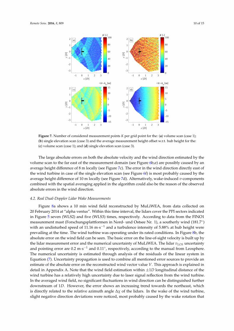
However, local errors can be noticed on the absolute error plots in Figure 6e,f, caused mainly bytwo reasons: the first issue is the intrinsically heterogeneous measurement distribution of the radialscan pattern of the lidars. Second, the average height at which measurements were taken causesa problem. Especially for the volume scan scenario, these two effects are entangled. Figure 7a,bshow the measurement distribution, i.e., the number of measurements K taken into account per gridpoint, for the two respective scenarios. Figure 7c,d illustrate the average offset from hub height of themeasurement set for each grid point.

The measurement distribution of the single elevation scan corresponds to the radial scanningpattern. Since the lidars are both located to the west, the distribution becomes less dense whenprogressing radially outward, i.e., from west to east. The measurement distribution of the volume scanis relatively heterogeneous due to the combination of multiple, partly overlapping PPI scans. However,it shows smaller absolute quantities than the single elevation scan and also has a larger spread in thecount of measurements over the grid. For the single elevation scan, the average height offset fromhub height is linearly increasing from west to radially outward. The volume scan approaches thehub height more convincingly, i.e., the average absolute offset of the measurements is much lower,namely 1.6 m instead of 6.8 m. However, due to the heterogeneous pattern, some local peaks and sharpdiscontinuities are present.

Remote Sens. 2016, 8, 809 10 of 15

-1 0 1 2 3x [D]

-3

-2

-1

0

1

2

y [D

]

a)

0

20

40

60

80

100K [-]

-1 0 1 2 3x [D]

-3

-2

-1

0

1

2

y [D

]

b)

0

20

40

60

80

100K [-]

-1 0 1 2 3x [D]

-3

-2

-1

0

1

2

y [D

]

c)

-15

-10

-5

0

5

10

15

<h>-hh [m]

-1 0 1 2 3x [D]

-3

-2

-1

0

1

2

y [D

]

d)

-15

-10

-5

0

5

10

15

<h>-hh [m]

Figure 7. Number of considered measurement points K per grid point for the: (a) volume scan (case 1);(b) single elevation scan (case 3) and the average measurement height offset w.r.t. hub height for the:(c) volume scan (case 1); and (d) single elevation scan (case 3).

The large absolute errors on both the absolute velocity and the wind direction estimated by thevolume scan to the far east of the measurement domain (see Figure 6b,e) are possibly caused by anaverage height difference of 8 m locally (see Figure 7c). The error in the wind direction directly east ofthe wind turbine in case of the single elevation scan (see Figure 6f) is most probably caused by theaverage height difference of 10 m locally (see Figure 7d). Alternatively, wake-induced v-componentscombined with the spatial averaging applied in the algorithm could also be the reason of the observedabsolute errors in the wind direction.

4.2. Real Dual-Doppler Lidar Wake Measurements

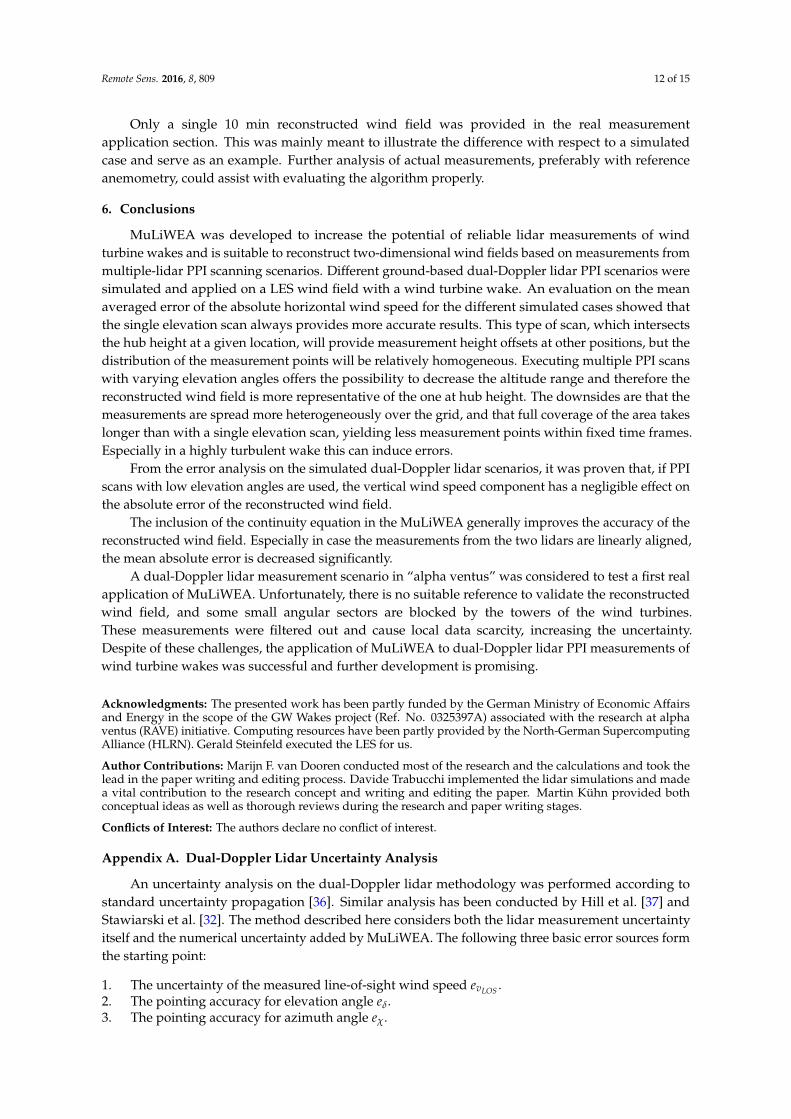
Figure 8a shows a 10 min wind field reconstructed by MuLiWEA, from data collected on20 February 2014 at “alpha ventus”. Within this time interval, the lidars cover the PPI sectors indicatedin Figure 5 seven (WLS2) and five (WLS3) times, respectively. According to data from the FINO1measurement mast (Forschungsplattformen in Nord- und Ostsee Nr. 1), a southerly wind (181.7◦)with an undisturbed speed of 11.16 m·s−1 and a turbulence intensity of 5.88% at hub height wereprevailing at the time. The wind turbine was operating under its rated conditions. In Figure 8b, theabsolute error on the wind field can be seen. The basic error on the line-of-sight velocity is built up bythe lidar measurement error and the numerical uncertainty of MuLiWEA. The lidar vLOS uncertaintyand pointing error are 0.2 m·s−1 and 0.11◦, respectively, according to the manual from Leosphere.The numerical uncertainty is estimated through analysis of the residuals of the linear system inEquation (7). Uncertainty propagation is used to combine all mentioned error sources to provide anestimate of the absolute error on the reconstructed wind vector value V. This approach is explained indetail in Appendix A. Note that the wind field estimation within ±1D longitudinal distance of thewind turbine has a relatively high uncertainty due to laser signal reflection from the wind turbine.In the averaged wind field, no significant fluctuations in wind direction can be distinguished furtherdownstream of 1D. However, the error shows an increasing trend towards the northeast, whichis directly related to the relative azimuth angle ∆χ of the lidars. In the wake of the wind turbine,slight negative direction deviations were noticed, most probably caused by the wake rotation that

Remote Sens. 2016, 8, 809 11 of 15

is impacting the horizontal wind speed at measurement heights above the hub height. More resultsfrom this measurement campaign were compared with LES by Vollmer et al. [35], which confirms theusefulness of the algorithm in combination with the measurement campaign for steady wake modelvalidation on a 10 min basis.

-1 0 1 2 3x [D]

0

1

2

3

4

5

y [

D]

a)

6

7

8

9

10

11

12

13V [m s-1]

-1 0 1 2 3x [D]

0

1

2

3

4

5

y [

D]

b)

0

0.1

0.2

0.3

0.4

0.5

eV [m s-1]

Figure 8. Reconstructed 10 min wind field on 20 February 2014 at 06:40:00 in the wind farm “alphaventus” with the wake of turbine AV10 (alpha ventus, number ten): (a) mean absolute velocity andvector field of the 2D velocity; and (b) calculated absolute error on the mean horizontal velocity.

5. Discussion

A problem with applying lidar to small scale meteorological phenomena is the spatial probelength averaging effect. In addition, the MuLiWEA performs spatial and temporal averaging of themeasurements. These effects combined hinder capturing large velocity gradients that commonly occuron the boundaries of wakes. However, the algorithm resolves the wake with sufficient accuracy todetermine e.g., its deficit and width. Because of the limitation on time resolution, it is not possibleto investigate wake or boundary layer dynamics with the scanning speed of the currently availablelidars using asynchronous PPI scans. This limitation could be overcome by synchronising the lidars orimproving their temporal resolution. In the current situation, the target application of the algorithm issteady wake model validation on a 10 min time scale.

The rotation of the near wake induces unsteady lateral and vertical wind speed components.This increases the uncertainty of a reconstructed wind field in case PPI scans are not executedhorizontally at hub height but with varying altitude offsets. In particular, a significant deviationwas observed in the wind direction for measurements taken at a distance from hub height. However,the effect on the absolute horizontal wind speed is negligible. Because the rotation of the wake isa deterministic phenomenon, it could be accounted for by the algorithm, in a similar way as thecontinuity adjustment was implemented.

Because the simulated lidar measurements were modeled to a perfect accuracy, most of theerrors in the investigated dual-Doppler lidar scenarios are indirectly a result of the irregular sampledistribution over the height, which does not perfectly resemble the hub height at all locations on thehorizontal plane.

Although it was argued and proven by the error analysis that neglecting the vertical velocitycomponent does not significantly increase the uncertainty of the reconstructed wind components,a valuable extension to MuLiWEA could be the inclusion of the vertical component. For this purpose,additional lidars are needed that measure with relatively high elevation angles.

Remote Sens. 2016, 8, 809 12 of 15

Only a single 10 min reconstructed wind field was provided in the real measurementapplication section. This was mainly meant to illustrate the difference with respect to a simulatedcase and serve as an example. Further analysis of actual measurements, preferably with referenceanemometry, could assist with evaluating the algorithm properly.

6. Conclusions

MuLiWEA was developed to increase the potential of reliable lidar measurements of windturbine wakes and is suitable to reconstruct two-dimensional wind fields based on measurements frommultiple-lidar PPI scanning scenarios. Different ground-based dual-Doppler lidar PPI scenarios weresimulated and applied on a LES wind field with a wind turbine wake. An evaluation on the meanaveraged error of the absolute horizontal wind speed for the different simulated cases showed thatthe single elevation scan always provides more accurate results. This type of scan, which intersectsthe hub height at a given location, will provide measurement height offsets at other positions, but thedistribution of the measurement points will be relatively homogeneous. Executing multiple PPI scanswith varying elevation angles offers the possibility to decrease the altitude range and therefore thereconstructed wind field is more representative of the one at hub height. The downsides are that themeasurements are spread more heterogeneously over the grid, and that full coverage of the area takeslonger than with a single elevation scan, yielding less measurement points within fixed time frames.Especially in a highly turbulent wake this can induce errors.

From the error analysis on the simulated dual-Doppler lidar scenarios, it was proven that, if PPIscans with low elevation angles are used, the vertical wind speed component has a negligible effect onthe absolute error of the reconstructed wind field.

The inclusion of the continuity equation in the MuLiWEA generally improves the accuracy of thereconstructed wind field. Especially in case the measurements from the two lidars are linearly aligned,the mean absolute error is decreased significantly.

A dual-Doppler lidar measurement scenario in “alpha ventus” was considered to test a first realapplication of MuLiWEA. Unfortunately, there is no suitable reference to validate the reconstructedwind field, and some small angular sectors are blocked by the towers of the wind turbines.These measurements were filtered out and cause local data scarcity, increasing the uncertainty.Despite of these challenges, the application of MuLiWEA to dual-Doppler lidar PPI measurements ofwind turbine wakes was successful and further development is promising.

Acknowledgments: The presented work has been partly funded by the German Ministry of Economic Affairsand Energy in the scope of the GW Wakes project (Ref. No. 0325397A) associated with the research at alphaventus (RAVE) initiative. Computing resources have been partly provided by the North-German SupercomputingAlliance (HLRN). Gerald Steinfeld executed the LES for us.

Author Contributions: Marijn F. van Dooren conducted most of the research and the calculations and took thelead in the paper writing and editing process. Davide Trabucchi implemented the lidar simulations and madea vital contribution to the research concept and writing and editing the paper. Martin Kühn provided bothconceptual ideas as well as thorough reviews during the research and paper writing stages.

Conflicts of Interest: The authors declare no conflict of interest.

Appendix A. Dual-Doppler Lidar Uncertainty Analysis

An uncertainty analysis on the dual-Doppler lidar methodology was performed according tostandard uncertainty propagation [36]. Similar analysis has been conducted by Hill et al. [37] andStawiarski et al. [32]. The method described here considers both the lidar measurement uncertaintyitself and the numerical uncertainty added by MuLiWEA. The following three basic error sources formthe starting point:

1. The uncertainty of the measured line-of-sight wind speed evLOS .2. The pointing accuracy for elevation angle eδ.3. The pointing accuracy for azimuth angle eχ.

Remote Sens. 2016, 8, 809 13 of 15

Both pointing accuracies are assumed to be 0.11◦ throughout the duration of the measurementcampaign. The measurement error on the line-of-sight velocity evLOS is assessed by taking into accountboth the lidar measurement accuracy from its user manual evLOSa

= 0.2 m·s−1 and the residuals of thematrix operation in Equation (7), which are used to give a numerical error estimate evLOSb

:

evLOS =√

e2vLOSa

+ e2vLOSb

. (A1)

The numerical uncertainty propagation of the MuLiWEA formalism is estimated assuming twolidars are synchronised. The two horizontal wind speed components are expressed as function of theradial velocities (see Equation (1)) of the two units (indicated by 1 and 2):

u =cos(χ1) cos(δ1)vLOS2 − cos(χ2) cos(δ2)vLOS1

cos(χ1) cos(δ1) sin(χ2) cos(δ2)− sin(χ1) cos(δ1) cos(χ2) cos(δ2), (A2)

v =sin(χ1) cos(δ1)vLOS2 − sin(χ2) cos(δ2)vLOS1

sin(χ1) cos(δ1) cos(χ2) cos(δ2)− cos(χ1) cos(δ1) sin(χ2) cos(δ2). (A3)

The numerical errors eu and ev are:

eu =

√(∂u

∂vLOS1evLOS1

)2+(

∂u∂vLOS2

evLOS2

)2+(

∂u∂χ1

eχ1

)2+(

∂u∂χ2

eχ2

)2+(

∂u∂δ1

eδ1

)2+(

∂u∂δ2

eδ2

)2, (A4)

ev =

√(∂v

∂vLOS1evLOS1

)2+(

∂v∂vLOS2

evLOS2

)2+(

∂v∂χ1

eχ1

)2+(

∂v∂χ2

eχ2

)2+(

∂v∂δ1

eδ1

)2+(

∂v∂δ2

eδ2

)2. (A5)

Finally, the absolute error eV on the absolute wind speed V is expressed as:

eV =√

e2u + e2

v. (A6)

References

1. Vermeer, L.J.; Sørensen, J.N.; Crespo, A. Wind Turbine Wake Aerodynamics. Prog. Aerosp. Sci. 2003,39, 467–510.

2. Barthelmie, R.J.; Hansen, K.; Frandsen, S.T.; Rathmann, O.; Schepers, J.G.; Schlez, W.; Phillips, J.; Rados, K.;Zervos, A.; Politis, E.S.; et al. Modelling and Measuring Flow and Wind Turbine Wakes in Large WindFarms Offshore. Wind Energy 2009, 12, 431–444.

3. Kusiak, A.; Song, Z. Design of Wind Farm Layout for Maximum Wind Energy Capture. Renew. Energy 2010,35, 685–694.

4. Gebraad, P.M.O.; van Wingerden, J.W. Maximum Power-Point Tracking Control for Wind Farms. Wind Energy2015, 18, 429–447.

5. Wandinger, U. Chapter 1—Introduction to Lidar. In Lidar—Range-Resolved Optical Remote Sensing of theAtmosphere; Springer: New York, NY, USA, 2005; pp. 1–18.

6. Werner, C. Chapter 12 - Doppler Wind Lidar. In Lidar—Range-Resolved Optical Remote Sensing of the Atmosphere;Springer: New York, NY, USA, 2005; pp. 325–354.

7. Smalikho, I.N.; Köpp, F.; Rahm, S. Measurement of Atmospheric Turbulence by 2-µm Doppler Lidar.J. Atmos. Ocean. Technol. 2005, 22, 1733–1747.

8. Wharton, S.; Newman, J.F.; Qualley, G.; Miller, W.O. Measuring Turbine Inflow With Vertically-ProfilingLidar in Complex Terrain. J. Wind Eng. Ind. Aerodyn. 2015, 142, 217–231.

9. Sathe, A.; Mann, J. A Review of Turbulence Measurements Using Ground-Based Wind Lidars.Atmos. Meas. Tech. 2013, 6, 3147–3167.

10. Bingöl, F.; Mann, J.; Larsen, G.C. Light Detection and Ranging Measurements of Wake Dynamics. Part I:One-Dimensional Scanning. Wind Energy 2010, 13, 51–61.

Remote Sens. 2016, 8, 809 14 of 15

11. Trujillo, J.J.; Bingöl, F.; Larsen, G.C.; Mann, J.; Kühn, M. Light Detection and Ranging Measurements ofWake Dynamics. Part II: Two-Dimensional Scanning. Wind Energy 2011, 14, 61–75.

12. Frehlich, R.; Hannon, S.M.; Henderson, S.W. Coherent Doppler Lidar Measurements of Wind Field Statistics.Bound.-Layer Meteorol. 1998, 86, 233–256.

13. Krishnamurthy, R.; Choukulkar, A.; Calhoun, R.; Fine, J.; Oliver, A.; Barr, K.S. Coherent Doppler Lidar forWind Farm Characterization. Wind Energy 2013, 16, 189–206.

14. Peña Diaz, A.; Hasager, C.B.; Lange, J.; Anger, J.; Badger, M.; Bingöl, F.; Bischoff, O.; Cariou, J.-P.;Dunne, F.; Emeis, S.; et al. Chapter 5: Pulsed Lidar. In Remote Sensing for Wind Energy; Number DTUWind Energy-E-Report-0029(EN); DTU Wind Energy: Roskilde, Denmark, 2013; pp. 131–148.

15. Käsler, Y.; Rahm, S.; Simmet, R.; Kühn, M. Wake Measurements of a Multi-MW Wind Turbine with CoherentLong-Range Pulsed Doppler Wind Lidar. J. Atmos. Ocean. Technol. 2010, 27, 1529–1532.

16. Aitken, M.L.; Banta, R.M.; Pichugina, Y.L.; Lundquist, J.K. Quantifying Wind Turbine Wake Characteristicsfrom Scanning Remote Sensor Data. J. Atmos. Ocean. Technol. 2014, 31, 765–787.

17. Banta, R.M.; Pichugina, Y.L.; Brewer, W.A.; Lundquist, J.K.; Kelley, N.D.; Sandberg, S.P.; Alvarez, R.J., II;Hardesty, R.M.; Weickmann, A.M. 3D Volumetric Analysis of Wind Turbine Wake Properties in theAtmosphere Using High-Resolution Doppler Lidar. J. Atmos. Ocean. Technol. 2015, 32, 904–914.

18. Iungo, G.V.; Wu, Y.; Porté-Agel, F. Field Measurements of Wind Turbine Wakes with Lidars. J. Atmos.Ocean. Technol. 2013, 30, 274–287.

19. Bousquet, O.; Chong, M. A Multiple-Doppler Synthesis and Continuity Adjustment Technique (MUSCAT) toRecover Wind Components from Doppler Radar Measurements. J. Atmos. Ocean. Technol. 1998, 15, 343–359.

20. Chong, M.; Campos, C. Extended Overdetermined Dual-Doppler Formalism in Synthesizing AirborneDoppler Radar Data. J. Atmos. Ocean. Technol. 1996, 13, 581–597.

21. Chong, M.; Bousquet, O. On The Application of MUSCAT to a Ground-Based Dual-Doppler Radar System.Meteorol. Atmos. Phys. 2001, 78, 133–139.

22. Drechsel, S.; Chong, M.; Mayr, G.J.; Weissmann, M.; Calhoun, R.; Dörnbrack, A. Three-Dimensional WindRetrieval: Application of MUSCAT to Dual-Doppler Lidar. J. Atmos. Ocean. Technol. 2009, 26, 635–646.

23. Hirth, B.D.; Schroeder, J.L.; Gunter, W.S.; Guynes, J.G. Coupling Doppler Radar-Derived Wind Maps withOperational Turbine Data to Document Wind Farm Complex Flows. Wind Energy 2015, 18, 529–540.

24. Newsom, R.K.; Calhoun, R.; Ligon, D.; Allwine, J. Linearly Organized Turbulence Structures Observed Overa Suburban Area by Dual-Doppler Lidar. Bound.-Layer Meteorol. 2008, 127, 111–130.

25. Cressman, G.P. An Operational Objective Analysis System. Mon. Weather Rev. 1959, 87, 367–374.26. Barnes, S.L. A Technique for Maximizing Details in Numerical Weather-Map Analysis. J. Appl. Meteorol.

1964, 3, 396–409.27. Cherukuru, N.W.; Calhoun, R.; Lehner, M.; Hoch, S.W.; Whiteman, C.D. Instrument Configuration for

Dual-Doppler Lidar Coplanar Scans: METCRAX II. J. Appl. Remote Sens. 2015, 9, 096090.28. Newsom, R.K.; Berg, L.K.; Shaw, W.J.; Fischer, M.L. Dual-Doppler Lidar for Measurement of Wind Turbine

Inflow-Outflow and Wake Effects. In Proceedings of the 50th AIAA Aerospace Sciences Meeting Includingthe New Horizons Forum and Aerospace Exposition, Nashville, TN, USA, 9–12 January 2012.

29. Kaw, A.; Kalu, E.E. Chapter 2—Differentiation of Continuous Functions. In Numerical Methods withApplications: Abridged; University of South Florida: Tampa, FL, USA, 2009; pp. 94–110.

30. Raasch, S.; Schröter, M. PALM—A Large-Eddy Simulation Model Performing on Massively ParallelComputers. Meteorol. Z. 2001, 10, 363–372.

31. Troldborg, N. Actuator Line Modeling of Wind Turbine Wakes. Ph.D. Thesis, Technical University ofDenmark, Lyngby, Denmark, 2008.

32. Stawiarski, C.; Träumner, K.; Knigge, C.; Calhoun, R. Scopes and Challenges of Dual-Doppler Lidar WindMeasurements—An Error Analysis. J. Atmos. Ocean. Technol. 2013, 30, 2044–2064.

33. Van Dooren, M.F. Analysis of Multiple-Doppler Lidar Data for the Characterization of Wakes in an OffshoreWind Farm. Master’s Thesis, ForWind—University of Oldenburg, Oldenburg, Germany, 2014.

34. Schneemann, J.; Trabucchi, D.; Trujillo, J.; Kühn, M. Comparing Measurements of the Horizontal WindSpeed of a 2D Multi-Lidar and a Cup Anemometer. J. Phys. Conf. Ser. 2014, 555, 012091.

35. Vollmer, L.; van Dooren, M.F.; Trabucchi, D.; Schneemann, J.; Steinfeld, G.; Witha, B.; Trujillo, J.J.; Kühn, M.First Comparison of LES of an Offshore Wind Turbine Wake With Dual-Doppler Lidar Measurements in aGerman Offshore Wind Farm. J. Phys. Conf. Ser. 2015, 625, doi:10.1088/1742-6596/625/1/012001.

Remote Sens. 2016, 8, 809 15 of 15

36. Joint Committee for Guides in Metrology (JCGM). Evaluation of Measurement Data: Guide to the Expressionof Uncertainty in Measurement; Technical Report; Joint Committee for Guides in Meteorology; BureauInternational des Poids et Mesures (BIPM): Sèvres, France, 2008.

37. Hill, M.; Calhoun, R.; Fernando, H.J.S.; Wieser, A.; Dörnbrack, A.; Weissmann, M.; Mayr, G.; Newsom, R.Coplanar Doppler Lidar Retrieval of Rotors from T-REX. J. Atmos. Sci. 2010, 67, 713–729.

c© 2016 by the authors; licensee MDPI, Basel, Switzerland. This article is an open accessarticle distributed under the terms and conditions of the Creative Commons Attribution(CC-BY) license (http://creativecommons.org/licenses/by/4.0/).