3-AXIS AND 5-AXIS MACHINING WITH STEWART PLATFORM NG …
240
3-AXIS AND 5-AXIS MACHINING WITH STEWART PLATFORM NG CHEE CHUNG (B. Eng. (Hons), NUS) A THESIS SUBMITTED FOR THE DEGREE OF DOCTOR OF PHILOSOPHY DEPARTMENT OF MECHANICAL ENGINEERING NATIONAL UNIVERSITY OF SINGAPORE 2012
Transcript of 3-AXIS AND 5-AXIS MACHINING WITH STEWART PLATFORM NG …
3-AXIS AND 5-AXIS MACHINING WITH STEWART
PLATFORM
NG CHEE CHUNG
(B. Eng. (Hons), NUS)
A THESIS SUBMITTED
FOR THE DEGREE OF DOCTOR OF PHILOSOPHY
DEPARTMENT OF MECHANICAL ENGINEERING
NATIONAL UNIVERSITY OF SINGAPORE
2012

i
Declaration
I hereby declare that this thesis is my original work and it has been written by me
in its entirety. I have duly acknowledged all
the sources of information which have been used in the thesis.
This thesis has also not been submitted for any degree in any university previously.
Ng Chee Chung
30 July 2012
Acknowledgements
ii
Acknowledgements
The author would like to express his sincere gratitude to Prof. Andrew Nee
Yeh Ching and Assoc. Prof. Ong Soh Khim for their assistance, inspiration and
guidance throughout the duration of this research project.
The author is also grateful to his fellow postgraduate students, Mr.
Vincensius Billy Saputra, Mr. Bernard Kee Buck Tong, Miss Wong Shek Yoon,
Mr. Stanley Thian Chen Hai and professional officer, Mr. Neo Ken Soon and Mr.
Tan Choon Huat for their constant encouragement and suggestions. Furthermore,
he is also grateful to Laboratory Technologist Mr. Lee Chiang Soon, Mr. Au Siew
Kong and Mr. Chua Choon Tye for their help in the fabrication of the components
and their advice in the design of the research project.
In addition, the author would like to acknowledge the assistance given by
the technical staff of the Advanced Manufacturing Laboratory, Mr. Wong Chian
Long, Mr. Simon Tan Suan Beng, Mr. Ho Yan Chee and Mr. Lim Soon Cheong.
Last but not least, the author would also like to acknowledge the financial
assistance received from National University of Singapore for the duration of the
project, and to thank all those who, directly or indirectly, have helped him in one
way or another.
Table of Contents
iii
Table of contents
Declaration…………………………………………………………………………i
Acknowledgements ................................................................................................. ii
Table of contents .................................................................................................... iii
Summary ................................................................................................................ iv
List of Tables.......................................................................................................... vi
List of Figures ....................................................................................................... vii
List of Symbols .................................................................................................... xiii
Chapter 1 Introduction ............................................................................................ 1
Chapter 2 Kinematics of Stewart Platform ........................................................... 13
Chapter 3 Fundamentals of Machining ................................................................. 39
Chapter 4 Three-Axis Machining.......................................................................... 50
Chapter 5 Five-axis machining ............................................................................. 76
Chapter 6 Five-axis machining post-processor ..................................................... 91
Chapter 7 Calibration of Stewart Platform.......................................................... 110
Chapter 8 Control interface ................................................................................. 124
Chapter 9 3-DOF modular micro Parallel Kinematic Manipulator for machining
............................................................................................................................. 130
Chapter 10 Conclusions and Recommendations ................................................. 160
References ........................................................................................................... 166
Appendices .......................................................................................................... 172
Appendix A: NC Code tables .............................................................................. 172
Appendix B: Coordinate of circular arc in NC program ..................................... 175
Appendix C: Sensors installation methods ......................................................... 184
Appendix D: Image processing ........................................................................... 200
Appendix E: Interval time calculation ................................................................ 219
Summary
iv
Summary
There is an increasing trend of interest to implement the Parallel
Kinematics Platforms (Stewart Platforms) in the fields of machining and
manufacturing. This is due to the capability of the Stewart Platforms to perform
six degrees-of-freedom (DOF) motions within a very compact environment,
which cannot be achieved by traditional machining centers.
However, unlike CNC machining centers which axes of movements can be
controlled individually, the movement of a Stewart Platform requires a
simultaneous control of the six individual links to achieve the final position of the
platform. Therefore, the available commercial CNC applications for the
machining centers are not suitable for use to control a Stewart Platform. A
specially defined postprocessor has to be developed to achieve automatic
conversion of CNC codes, which have been generated from commercial CAM
packages based on the CAD models, to control and manipulate a Stewart Platform
to achieve the machining purposes. Furthermore, a sophisticated control interface
has been developed so that users can perform machining with a Stewart Platform
based on CNC codes.
Calibration of the accuracy of the developed NC postprocessor program
has been performed based on actual 3-axis and 5-axis machining processes
performed on the Stewart Platform. A machining frame with a spindle was
designed and developed, and a feedback system was implemented based on wire
Summary
v
sensors mounted linearly along the actuators of the platform. Thus, the position
and orientation of the end-effector can be calibrated based on the feedback of the
links of the platform. Experimental data was collected during the machining
processes. The data was analyzed and improvement was made on the
configuration of the system.
Alternate machining processes are reviewed with Parallel Kinematic
Manipulators of different structural designs that have been used for the Stewart
Platform. The structural characteristics associated with parallel manipulators are
evaluated. A class of three DOF parallel manipulators is determined. Several types
of parallel manipulators with translational movement and orientation have been
identified. Based on the identification, a hybrid 3-.UPU (Universal Joint-
Prismatic-Universal Joint) parallel manipulator was fabricated and studied.

List of Tables
vi
List of Tables
Table 3.1 Characteristic of various structure concepts [Reimund, 2000] ............. 43
Table 3.2 Comparison of workspace of CNC machine and Stewart Platform...... 45
Table 4.1 Coordinate systems ............................................................................... 52
Table 9.1 Feasible limb configurations for spatial 3-DOF manipulators [Tsai,
2000] ................................................................................................................... 133
Table 9.2 Workspace of mobile platforms with various radii ............................. 137
Table 9.3 Workspace of the base with various radii ........................................... 138
Table 9.4 Calibration Result of the Micro Stewart Platform with the CMM ..... 155
Table 9.5 Calibration Result of the Micro Stewart Platform with the CMM when
the Platform travels within boundary workspace ................................................ 157
Table A1 Address characters [Ken, 2001] .......................................................... 172
Table A2 G-codes chart [Ken, 2001] .................................................................. 173
Table A3 Miscellaneous functions (M functions) [Ken, 2001] .......................... 174
Table D1 Difference of displacement value of each actuator corresponding to
100,000 counts of pulse of the stepper motor ..................................................... 213
Table D2 Error of motion along the Z-axis ......................................................... 215
Table D3 Coordinate of the calibrated Points ..................................................... 217
Table E1 Previous data collected by manually moving the Stewart Platform .... 222
Table E2 The time calculation when the velocity is 50000 step/sec and the
acceleration is 500000 step/sec2 .......................................................................... 222
List of Figures
vii
List of Figures
Figure 1.1 Serial kinematics chains [Irene and Gloria, 2000] ................................ 3
Figure 1.2 Parallel kinematics manipulator classifications ..................................... 5
Figure 1.3 The standard Stewart Platform [Craig, 1986] ........................................ 7
Figure 1.4 Stewart Platform machining center ....................................................... 9
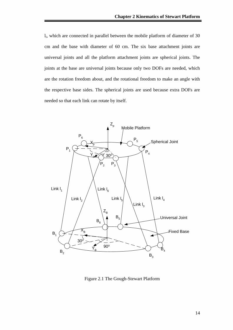
Figure 2.1 The Gough-Stewart Platform ............................................................... 14
Figure 2.2 Locations of the joints of the platform ................................................ 16
Figure 2.3 Locations of the joints of the base ....................................................... 16
Figure 2.4 The workspace of Stewart Platform when ........... 32
Figure 2.5 The algorithm of the workspace calculation ........................................ 33
Figure 2.6 The singularity configuration of Stewart Platform [Yee, 1993] .......... 37
Figure 3.1 Standard postprocessor sequences ....................................................... 41
Figure 3.2 CNC model inputs/outputs schematic representation .......................... 42
Figure 3.3 Comparison of the workspace of Stewart Platform (blue color dots) and
CNC machine (red color lines) ............................................................................. 44
Figure 3.4(a) Dexterous workspace (red color box) of the Stewart Platform (Front)
............................................................................................................................... 46
Figure 3.4(b) Dexterous workspace (red color box) of the Stewart Platform (Side)
............................................................................................................................... 46
Figure 4.1 The coordinate system of a Stewart Platform ...................................... 50
Figure 4.2 Comparison of the coordinate systems of the cutting tool and the
Stewart Platform.................................................................................................... 51
Figure 4.3 Cutting tool and platform movements during the machining process for
Stewart Platform.................................................................................................... 52
Figure 4.4 Format of an NC program ................................................................... 56
Figure 4.5 Flow chart of identification algorithm to evaluate address characters
and the respective values ....................................................................................... 58
Figure 4.6(a) Flow chart of algorithm to determine maximum number of G code59
Figure 4.6(b) Flow chart of algorithm to determine maximum number of M code
............................................................................................................................... 60
Figure 4.7 Flow chart of matrix preparation for the corresponding character
address of an NC program .................................................................................... 62
Figure 4.8 Flow chart of algorithm to assign the value of character addresses of an
NC program to the respective character addresses matrix array ........................... 63
Figure 4.9 Flow chart of algorithm to determine the characteristics of the
coordinate system .................................................................................................. 65
Figure 4.10 Flow chart of algorithm to determine the values of X-, Y- and Z-
coordinates ............................................................................................................ 66
0,0,0
List of Figures
viii
Figure 4.11 Flow chart of algorithm to determine the cutting plane and the style of
the cutting path ...................................................................................................... 68
Figure 4.12(a) Flow chart of algorithm to convert NC program to machine
trajectory ............................................................................................................... 69
Figure 4.12(b) Flow chart of algorithm to convert NC program to the machine
trajectory ............................................................................................................... 70
Figure 4.13 Trajectory path of a Stewart Platform translated from an NC program
............................................................................................................................... 71
Figure 4.14(a) The pocketing machining process: plot outline in MasterCam ..... 72
Figure 4.14(b) The pocketing process: MasterCam generate the tool cutting path
............................................................................................................................... 72
Figure 4.14(c) The pocketing process: Simulation of cutting path in MasterCam 73
Figure4.14(d) The pocketing process: Generate trajectory path ........................... 73
through MATLAB®
.............................................................................................. 73
Figure 4.14(e) The pocketing process: Machine workpiece through the contouring
process ................................................................................................................... 74
Figure 4.15 3D cutting path generated from the NC program created from model
in MasterCam ........................................................................................................ 75
Figure 4.16 Outcome of machining on a Stewart Platform .................................. 75
Figure 5.1 Geometric error associated with tolerance between freeform surface
and designed surface ............................................................................................. 77
Figure 5.2 A constant step over distance in the parametric space does not
generally yield a constant step over in the Cartesian space [Liang, 2002] ........... 78
Figure 5.3 Triangular tessellated freeform surface ............................................... 79
Figure 5.4 Standard triangular representation of STL model ............................... 80
Figure 5.5 Generation of CC points ...................................................................... 83
Figure 5.6 Determination of the intersection points between the cutting plane and
the face on the freeform surface ............................................................................ 85
Figure 5.7(a) Flow chart for the generation of CC points ..................................... 86
Figure 5.7(b) Flow chart for the generation of CC points .................................... 87
Figure 5.8 Local Coordinate System (LCS) Setup ............................................... 88
Figure 5.9 Collision between tool and freedom surface ....................................... 89
Figure 5.10 Gouging ............................................................................................. 90
Figure 6.1 Comparison of (a) 5-axis machining center and (b) Stewart Platform 92
Figure 6.2 Various coordinate systems defined in the Stewart Platform .............. 93
Figure 6.3 Orientation of mobile platform around Y-axis .................................... 95
Figure 6.4 Relationship between the cutting tool frame LCS and the workpiece
frame LCS ............................................................................................................. 97
List of Figures
ix
Figure 6.5 Normal Vector of Face intersected with the Cutting Plane ................. 99
Figure 6.6 ASCII STL text format ...................................................................... 101
Figure 6.7 The surface model derived from the vertices and faces .................... 101
Figure 6.8 Tessellated triangular surfaces of the freeform surface ..................... 102
Figure 6.9 Intersected points with norm (green dot line) along the cutting plane
............................................................................................................................. 103
Figure 6.10 Intersected points of the freeform surface with one cutting plane and
perpendicular lines (green) are the normal of the intersected points .................. 104
Figure 6.11 Generation of the intersected points with a series of cutting planes 105
Figure 6.12 Generation of the intersected points with a series of cutting planes 106
Figure 6.13 Trajectory path of the Stewart Platform generated based on the LCS
of the freeform surface ........................................................................................ 107
Figure 6.14 Trajectory path of the Stewart Platform with retracted points ........ 107
Figure 6.15 Simulation of 5-axis machining in MATLAB®
............................... 108
Figure 6.16 5-axis machining result .................................................................... 109
Figure 7.1 The mounting of the sensors to the sensor holder ............................. 111
Figure 7.2 The model of the trajectory path of the end-effector based on the
feedback of the wire sensors while the platform was moving along the Z-axis . 112
Figure 7.3 The model of the trajectory path of the end-effector based on the
feedback of the wire sensors while the platform was moving along the Z-axis
(front view).......................................................................................................... 113
Figure 7.4 The model of the trajectory path of the end-effector based on the
feedback of the wire sensors while the platform was moving along the X-axis . 114
Figure 7.5 The model of the trajectory path of the end-effector based on the
feedback of the wire sensors while the platform was moving along the Y-axis . 115
Figure 7.6 Feedback of actuators stroke position while the platform is ............. 117
being manipulated. .............................................................................................. 117
Figure 7.7 The corresponding position and orientation of the platform end-effector
with respect to the strokes of the actuators ......................................................... 118
Figure 7.8 The Stewart Platform position and orientation feedback interface ... 119
Figure 7.9 The real time feedback interface of the wire sensor when the platform
is being manipulated ........................................................................................... 120
Figure 7.10 The tool path generated from the real time position feedback ........ 120
Figure 7.11 Calibration of workpiece ................................................................. 121
Figure 7.12 Comparison of calibrated result of the plotted point (Blue) and the
ideal point (Red) and the coordinate of the plotted points on the calibration plate
............................................................................................................................. 122
Figure 8.1 Motion control interface .................................................................... 125
Figure 8.2 Motion control feedback .................................................................... 126
List of Figures
x
Figure 8.3 Wire sensor interface ......................................................................... 127
Figure 8.4 NC program Interface ........................................................................ 128
Figure 8.5 OpenGL Interface .............................................................................. 129
Figure 9.1(a)(b) 6-Legged Micro Stewart Platform and 3-Legged Micro Stewart
Platform (c) PSU Micro Stewart Platform .......................................................... 135
Figure 9.2 Comparison of Workspace of 3-legged (red) and 6-legged (blue)
Parallel Manipulator ............................................................................................ 136
Figure 9.3 Workspace VS radius of Mobile Platform......................................... 137
Figure 9.4 Workspace vs Radius of Base ........................................................... 138
Figure 9.5 The workspace comparison between Passive Joint angle of 20º and 45º
............................................................................................................................. 140
Figure 9.6 The M-235.5 DG Actuator and Hephaist Seiko Spherical Joint ....... 142
Designs of the Micro Parallel Manipulator ......................................................... 142
Figure 9.7 Parallel Manipulator system fabricated using the same modular
components (Prismatic Actuator, Spherical Joints, Universal Joints and Variable
Links) .................................................................................................................. 143
Figure 9.8 (a) Pure Translational Platform, (b) Pure Rotational Platform .......... 146
Figure 9.9 Hybrid UPU Parallel Kinematic Manipulator ................................... 147
Figure 9.10 Schematic Diagram of the Parallel Kinematics Platform (PKM) .... 148
Figure 9.11 Calculation of the actual stroke of the link ...................................... 149
Figure 9.12 Denavit-Hartenberg Representation ................................................ 150
Figure 9.13 The UPU Modified Stewart Platform with a passive prismatic middle
link ...................................................................................................................... 151
Figure 9.14 The Relationship between the Surface Point and the spherical joint152
Figure 9.15 Workspace of the Surface Point of the Hybrid PKM ...................... 153
Figure 9.16 Accuracy Calibration of the Micro Stewart Platform with CMM ... 154
Figure 9.17 Displacement and Rotational Error Analysis .................................. 156
Figure 9.18 Integration of the hybrid 3-DOF PKM into 3-axis machining center
............................................................................................................................. 159
Figure 9.19 The machined workpiece ................................................................. 159
Figure 10.1 The theodolites system based on the principle of triangulation ...... 164
Figure B1 Generic circular arc motion of the machining point in one plane ...... 176
Figure B2 Clockwise circular arc motion with angle of starting point θ smaller
than angle of ending point β with respect to reference point .............................. 178
Figure B3 Clockwise circular arc motion with angle of ending point smaller than
angle of starting point with referred to reference point....................................... 178
Figure B4 Clockwise circular arc motion with starting point at the right side and
ending point at the left side of the reference point .............................................. 179
List of Figures
xi
Figure B5 Clockwise circular arc motion with starting point at the left side and
ending point at the right side of the reference point............................................ 180
Figure B6 Clockwise circular arc motion with starting point and ending point at
the left side of the reference point with angle theta larger than angle beta ......... 181
Figure B7 Clockwise circular arc motion with starting point and ending point at
the left side of the reference point with angle theta smaller than angle beta ...... 182
Figure C1 The developed Stewart Platform and the Epsilon wire sensor........... 184
Figure C2 The MATLAB® simulation of the forward kinematics calibration
system .................................................................................................................. 186
Figure C3 The laser pointer calibration system diagram .................................... 187
Figure C4 The MATLAB® simulation of the laser platform calibration system 189
Figure C5 The wire sensor calibration system diagram ...................................... 191
Figure C6 Cartesian Coordinate of the vector points .......................................... 193
Figure C7 The calibration setup for wire sensor ................................................. 195
Figure C8 Graph of Comparison between theoretical data and actual data from
Multimeter ........................................................................................................... 196
Figure C9 Graph of Actual Length vs Voltage of the wire sensor...................... 197
Figure C10 Wire sensor interface ....................................................................... 198
............................................................................................................................. 198
Figure C11 The Sampled Wave Signal of the wire sensors ................................ 198
Figure D1 The original image with marked points ............................................. 200
Figure D2 Black and white image ....................................................................... 201
Figure D3 the Image is rotated into the position so that it is in line with the
horizontal level .................................................................................................... 202
Figure D4 Calibrated points of the image in terms of red color for the printed
point and blue color highlighted dots for the points marked by the pen ............. 202
Figure D5 the tilted line (in green) plotted with respected to the marked points in
the middle of the graph ....................................................................................... 203
Figure D6a All three sets of coordinates of the Printed Points (Red), Marked
Points (Blue) and Modified Points (Green) ........................................................ 204
Figure D6b All three sets of coordinates without background image ................. 205
Figure D7 the errors of calibrated points along the X-axis ................................. 206
Figure D8 the errors of calibrated points along the Y-axis ................................. 207
Figure D9(a) the distance between two adjacent points along the X-axis .......... 208
Figure D9(b) the distance between two adjacent points along the Y-axis .......... 209
Figure D10 The unevenness of the points motion even though it is moving ...... 210
in the X-direction ................................................................................................ 210

List of Figures
xii
Figure D11 The corresponding error resulting from the ratio of actuator movement
over the counter of 100,000 steps from the controller ........................................ 212
Figure D12 The LVDT-like device ..................................................................... 214
Figure D13 Calibrated Workpiece ...................................................................... 216
Figure D14 The comparison of coordinates between the actual calibrated points
and the theoretical points .................................................................................... 218
Figure E1 Distance, Velocity and Acceleration Diagram ................................... 220
Figure E2 Flow chart of the interval time control ............................................... 223
List of Symbols
xiii
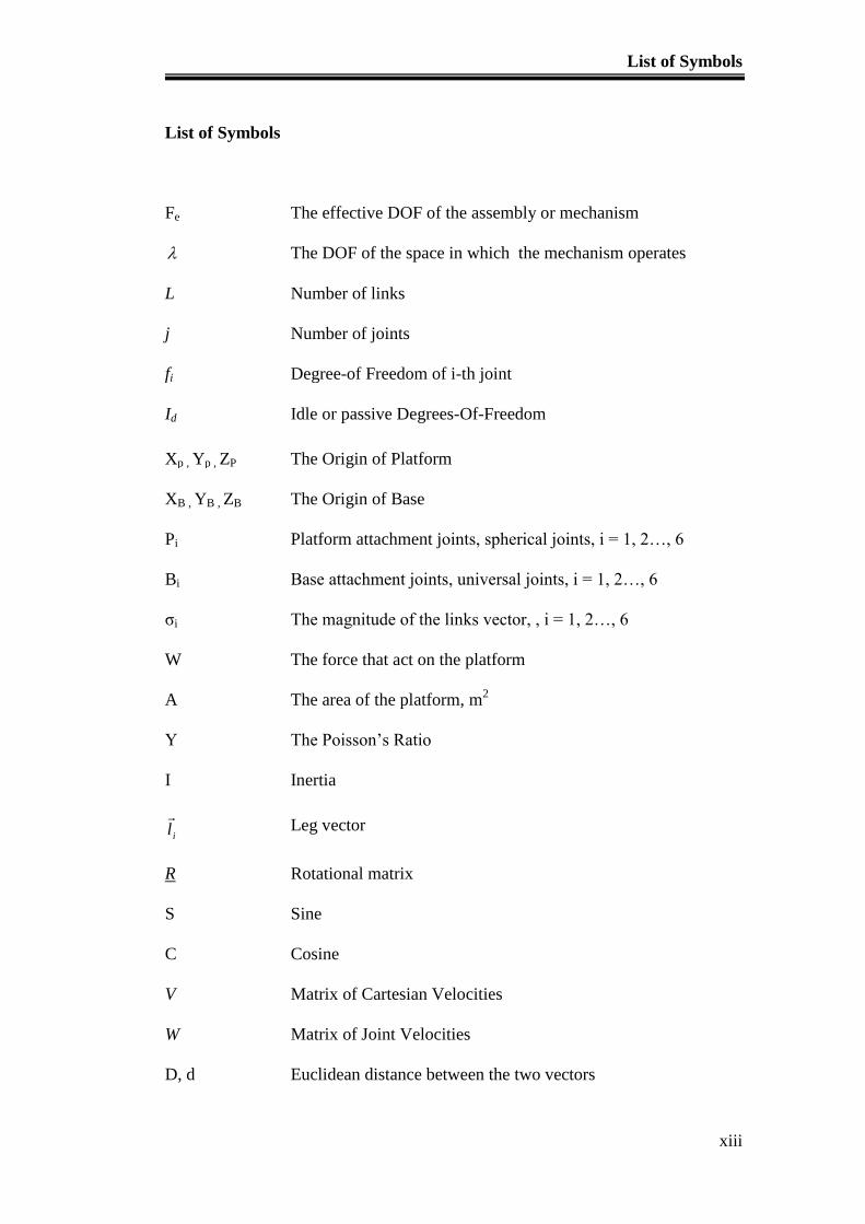
List of Symbols
Fe The effective DOF of the assembly or mechanism
The DOF of the space in which the mechanism operates
L Number of links
j Number of joints
fi Degree-of Freedom of i-th joint
Id Idle or passive Degrees-Of-Freedom
Xp , Yp , ZP The Origin of Platform
XB , YB , ZB The Origin of Base
Pi Platform attachment joints, spherical joints, i = 1, 2…, 6
Bi Base attachment joints, universal joints, i = 1, 2…, 6
σi The magnitude of the links vector, , i = 1, 2…, 6
W The force that act on the platform
A The area of the platform, m2
Υ The Poisson’s Ratio
I Inertia
Leg vector
R Rotational matrix
S Sine
C Cosine
V Matrix of Cartesian Velocities
W Matrix of Joint Velocities
D, d Euclidean distance between the two vectors
il
List of Symbols
xiv
NaN Not a Numerical number
Rot3x3 3 x 3Rotation matrix of Stewart Platform
Tr3x1 3 x 1Translational matrix of Stewart Platform
T Homogeneous Coordinate
Ξ Tolerance of Error
t
Translational Vector
iX
Matrix of pose vector of Stewart Platform
G Mapping function of length of actuators to the pose of the
Stewart Platform
H Differentiation of Mapping function G with the corresponding
element of the pose vector of Stewart Platform
Rxyz Rotation matrix around X-axis, Y-axis and Z-axis
Rz,α Rotation matrix around Z axis with rotational angle of α
Ry,β Rotation matrix around Y axis with rotational angle of β
Rz,γ Rotation matrix around Z axis with rotational angle of γ
Az Area of the workspace of Stewart Platform
V Volume of Workspace
fbi Force acting on the spherical joint of the mobile platform
fai Force acting on the universal joint of the base of Stewart
Platform
ωp Angular velocity of the mobile platform
ini Moment acting on the actuator
m1
Mass of cylinder of actuator
m2 Mass of piston of actuator
List of Symbols
xv
e1i Distance between the center of mass of the cylinder and the
bottom of the cylinder
e2i Distance between the center of mass of the piston and the top of
the piston
v1,v2 Velocity of the center of mass of the cylinder and piston
Bnp Moment about the center of mass of the mobile platform
i Actuating force of the platform
X_platform,
Y_platform,
Z_platform
Coordinates of mobile platform in local coordinate system
X_CNC_Code,
Y_CNC_Code,
Z_CNC_Code
Coordinate of XYZ coordinates in NC program
Xabs,Yabs,Zabs Absolute coordinate of X, Y and Z position of the mobile
platform
Xrel,Yrel,Zrel Relative coordinate of X, Y and Z position of the mobile
platform
C Vector between cutter contact point and normal N of the
triangular faces of the freeform surface
N Vector of normal to the face of the triangle in the freeform
surface
αc Critical angle of Collision
α1, α2 Critical angle of gouging
Vmw Vector from milling cutter to workpiece
NR Magnitude of vector of the normal to the triangle face of the
freeform surface
Chapter 1 Introduction
1
Chapter 1 Introduction
Parallel manipulators can be found in many applications in the industry,
such as vehicle and airplane simulators [Stewart, 1965], adjustable articulated
trusses [Reinholtz and Gockhale, 1987], mining machines [Arai et al, 1991],
positioning devices [Gosselin and Hamel, 1994], fine positioning devices, and off-
shore drilling platforms. Recently, it has also been developed as high precision
milling machines, namely, a hexapod machining center by Giddings and Lewis in
1995. A Stewart Platform is a form of manipulator with six degrees of freedoms
(DOF), which allows one to provide a given position and orientation of the
surface in the vicinity of any point of the platform on its three Cartesian
coordinates and projection of the unit of normal vector [Alyushin, 2010].
The design of parallel manipulators can be dated back to 1962 when
Gough and Whitehall [Gough, 1962] devised a six-linear jacking system for use as
a universal tire testing machine. Stewart presented his platform manipulator for
use as an aircraft simulator in 1965 [Stewart, 1965]. Hunt made a systematic study
of the parallel manipulator structures [Hunt, 1983]. Since then, parallel
manipulators have been studied extensively by many other researchers [Tsai,
1996].
However, greater interests in the application of these mechanisms in the
metalworking field have only grown in the last decade. The first CNC-type
hexapod machine tool prototype (Variax from Giddings & Lewis and the
Chapter 1 Introduction
2
Octahedral Hexapod from Ingersoll) was presented at the 1994 International
Machine Tool Show in Chicago. These prototypes were enthusiastically
welcomed as the new generation of machine tools due to their specific
characteristics [Irene and Gloria, 2000]:
Higher payload to weight ratio
Non-cumulative joint error
Higher structural rigidity
Modularity
Location of the motors close to the fixed base
Simpler solution of the ‘inverse’ kinematics problem
However, there are still many disadvantages of the Stewart Platform as
compared to the serial manipulators, such as a limited workspace and problems in
singularity configuration. Furthermore, it also has complicated forward kinematics
due to the closed loop configuration of the system.
Configuration and classification
Most of the robots being used in the industries today are serial robots or
serial manipulators. Manipulators are basically mechanical motion devices,
generally with two or more DOF. Serial manipulators are normally made up of
between two to six rigid links with prismatic and/or revolute joints connecting the
links in an open kinematics chain. Examples of this kind of robots include the
PUMA 560 series of robot arm and the SCARA type Adept One robot arm [Yee
1993].
Chapter 1 Introduction
3
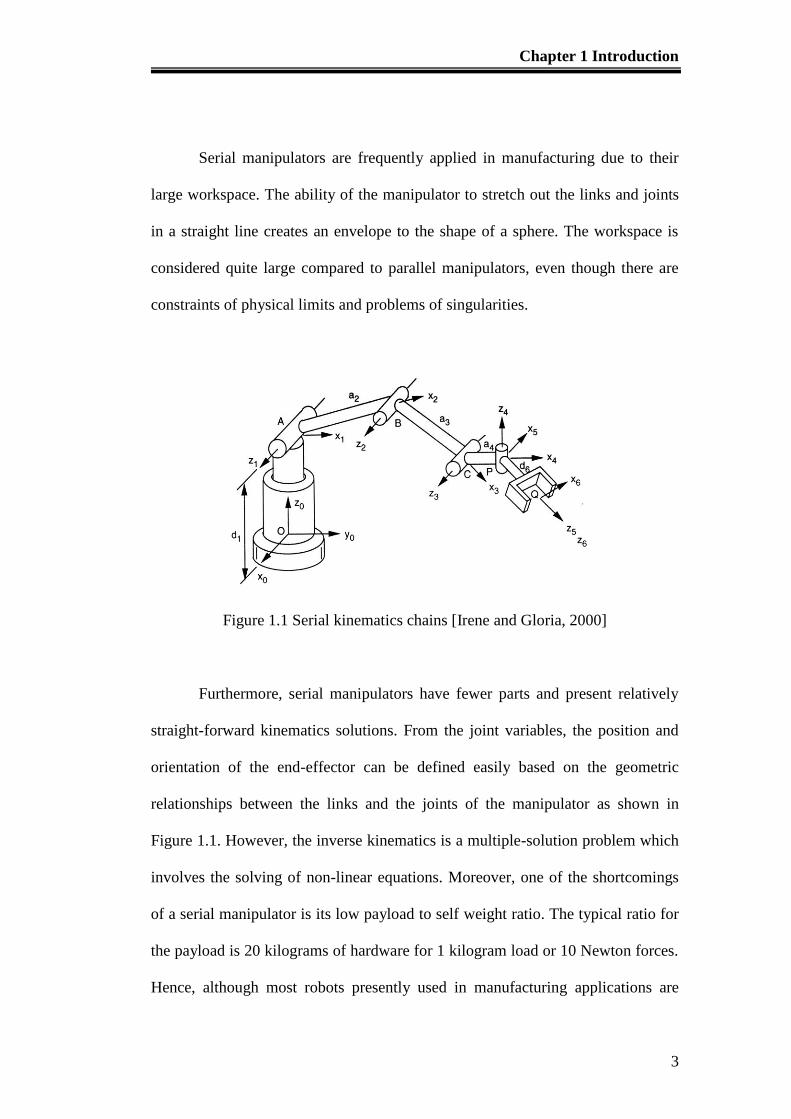
Serial manipulators are frequently applied in manufacturing due to their
large workspace. The ability of the manipulator to stretch out the links and joints
in a straight line creates an envelope to the shape of a sphere. The workspace is
considered quite large compared to parallel manipulators, even though there are
constraints of physical limits and problems of singularities.
Figure 1.1 Serial kinematics chains [Irene and Gloria, 2000]
Furthermore, serial manipulators have fewer parts and present relatively
straight-forward kinematics solutions. From the joint variables, the position and
orientation of the end-effector can be defined easily based on the geometric
relationships between the links and the joints of the manipulator as shown in
Figure 1.1. However, the inverse kinematics is a multiple-solution problem which
involves the solving of non-linear equations. Moreover, one of the shortcomings
of a serial manipulator is its low payload to self weight ratio. The typical ratio for
the payload is 20 kilograms of hardware for 1 kilogram load or 10 Newton forces.
Hence, although most robots presently used in manufacturing applications are
Chapter 1 Introduction
4
serial manipulators, parallel manipulators clearly excel in the aspects of stiffness,
inertia, accuracy and payload [Vincent, 2001].
The parallel structures are classified according to the types of drives. This
classification is not limited to the DOF, and hence the design of the joints is not
restricted by the classification. As a result, rotary and translational drives can both
be used [Reimund, 2002]. Among the types of drives used, rotary drives show a
high degree of efficiency. With the installation of a gear system, the rotation
motion can be converted to translation motion. Hence, ball screws are chosen for
the gear conversion. Furthermore, other driver principles, such as pneumatic or
hydraulic system can apply direct linear motion or indirect motion towards the
parallel kinematics manipulator systems.
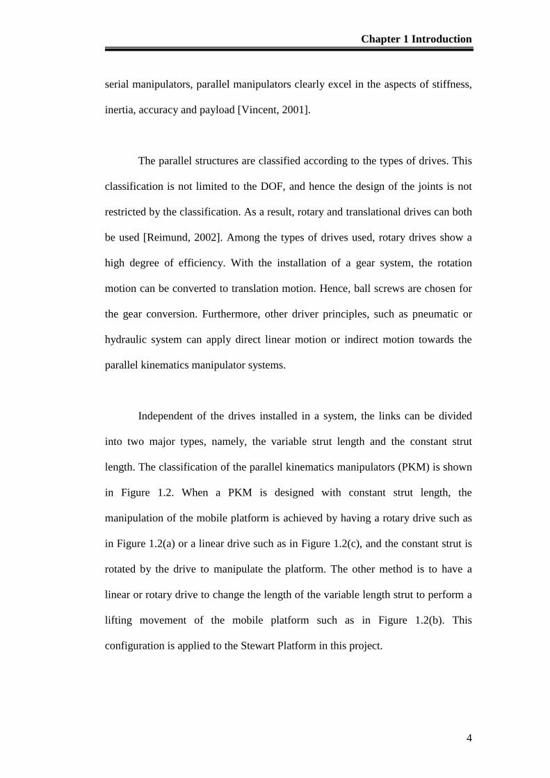
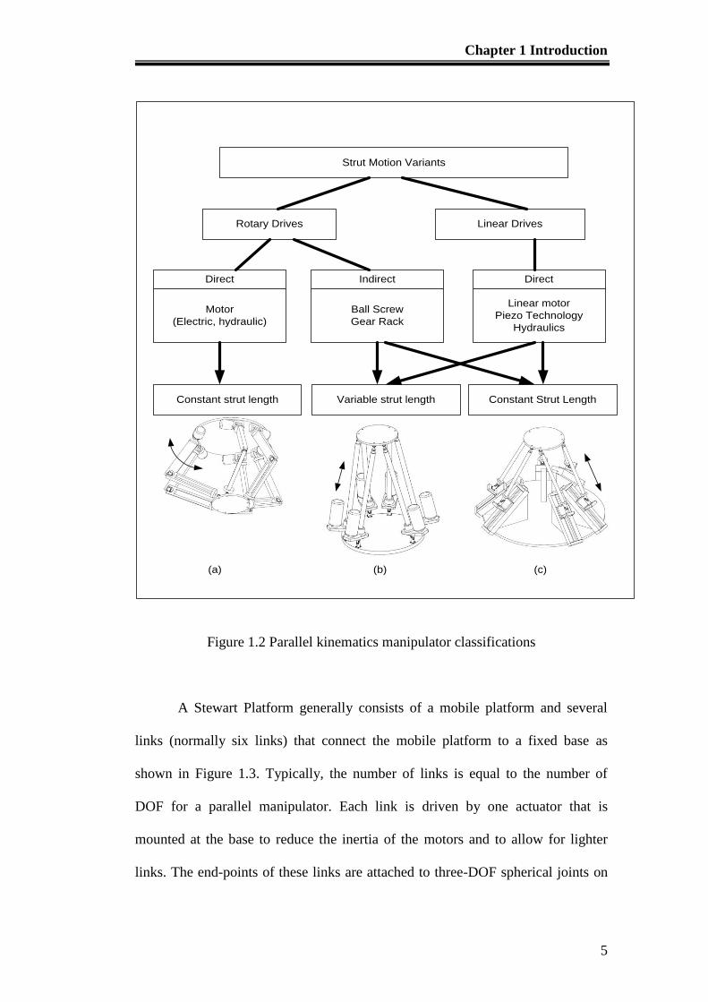
Independent of the drives installed in a system, the links can be divided
into two major types, namely, the variable strut length and the constant strut
length. The classification of the parallel kinematics manipulators (PKM) is shown
in Figure 1.2. When a PKM is designed with constant strut length, the
manipulation of the mobile platform is achieved by having a rotary drive such as
in Figure 1.2(a) or a linear drive such as in Figure 1.2(c), and the constant strut is
rotated by the drive to manipulate the platform. The other method is to have a
linear or rotary drive to change the length of the variable length strut to perform a
lifting movement of the mobile platform such as in Figure 1.2(b). This
configuration is applied to the Stewart Platform in this project.
Chapter 1 Introduction
5
Strut Motion Variants
Rotary Drives Linear Drives
Motor
(Electric, hydraulic)
Direct
Ball Screw
Gear Rack
Indirect
Linear motor
Piezo Technology
Hydraulics
Direct
Constant strut length Variable strut length Constant Strut Length
(a) (b) (c)
Figure 1.2 Parallel kinematics manipulator classifications
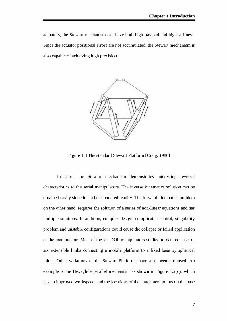
A Stewart Platform generally consists of a mobile platform and several
links (normally six links) that connect the mobile platform to a fixed base as
shown in Figure 1.3. Typically, the number of links is equal to the number of
DOF for a parallel manipulator. Each link is driven by one actuator that is
mounted at the base to reduce the inertia of the motors and to allow for lighter
links. The end-points of these links are attached to three-DOF spherical joints on
Chapter 1 Introduction
6
one end, and two-DOF universal joints on the other end. The position and
orientation of the mobile platform are controlled by the lengths of the prismatic
linear actuators. The Stewart mechanism depicts a closed loop alternative to the
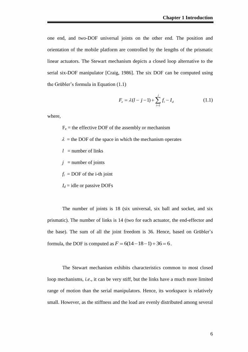
serial six-DOF manipulator [Craig, 1986]. The six DOF can be computed using
the Grübler’s formula in Equation (1.1)
(1.1)
where,
Fe = the effective DOF of the assembly or mechanism
= the DOF of the space in which the mechanism operates
l = number of links
j = number of joints
fi = DOF of the i-th joint
Id = idle or passive DOFs
The number of joints is 18 (six universal, six ball and socket, and six
prismatic). The number of links is 14 (two for each actuator, the end-effector and
the base). The sum of all the joint freedom is 36. Hence, based on Grübler’s
formula, the DOF is computed as .
The Stewart mechanism exhibits characteristics common to most closed
loop mechanisms, i.e., it can be very stiff, but the links have a much more limited
range of motion than the serial manipulators. Hence, its workspace is relatively
small. However, as the stiffness and the load are evenly distributed among several
j
i
die IfjlF1
)1(
636)11814(6 F
Chapter 1 Introduction
7
actuators, the Stewart mechanism can have both high payload and high stiffness.
Since the actuator positional errors are not accumulated, the Stewart mechanism is
also capable of achieving high precision.
Figure 1.3 The standard Stewart Platform [Craig, 1986]
In short, the Stewart mechanism demonstrates interesting reversal
characteristics to the serial manipulators. The inverse kinematics solution can be
obtained easily since it can be calculated readily. The forward kinematics problem,
on the other hand, requires the solution of a series of non-linear equations and has
multiple solutions. In addition, complex design, complicated control, singularity
problem and unstable configurations could cause the collapse or failed application
of the manipulator. Most of the six-DOF manipulators studied to-date consists of
six extensible limbs connecting a mobile platform to a fixed base by spherical
joints. Other variations of the Stewart Platforms have also been proposed. An
example is the Hexaglide parallel mechanism as shown in Figure 1.2(c), which
has an improved workspace, and the locations of the attachment points on the base
Chapter 1 Introduction
8
and on the mobile platform are not in a plane and are not symmetrical. There are
advantages and disadvantages of the various types of Stewart Platform designs.
The Gough-Stewart Platform, which has the smallest workspace, was
chosen as the design model because it has the most balanced performance [Huynh,
2001].
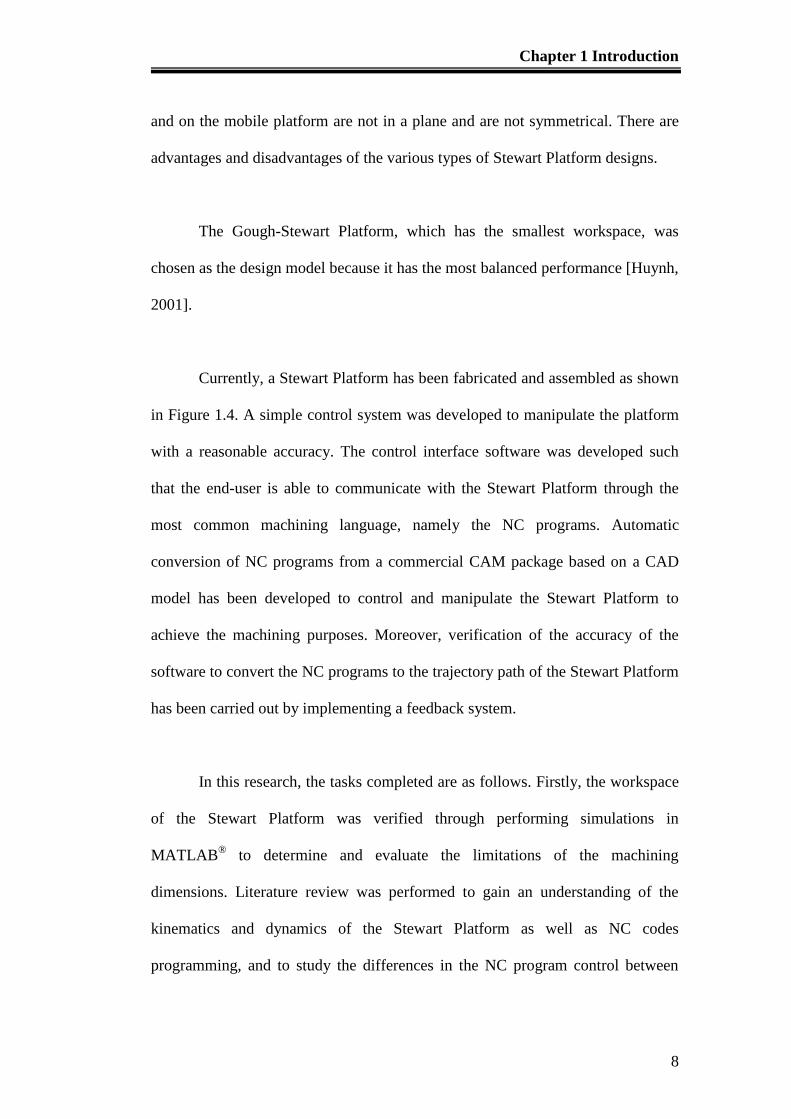
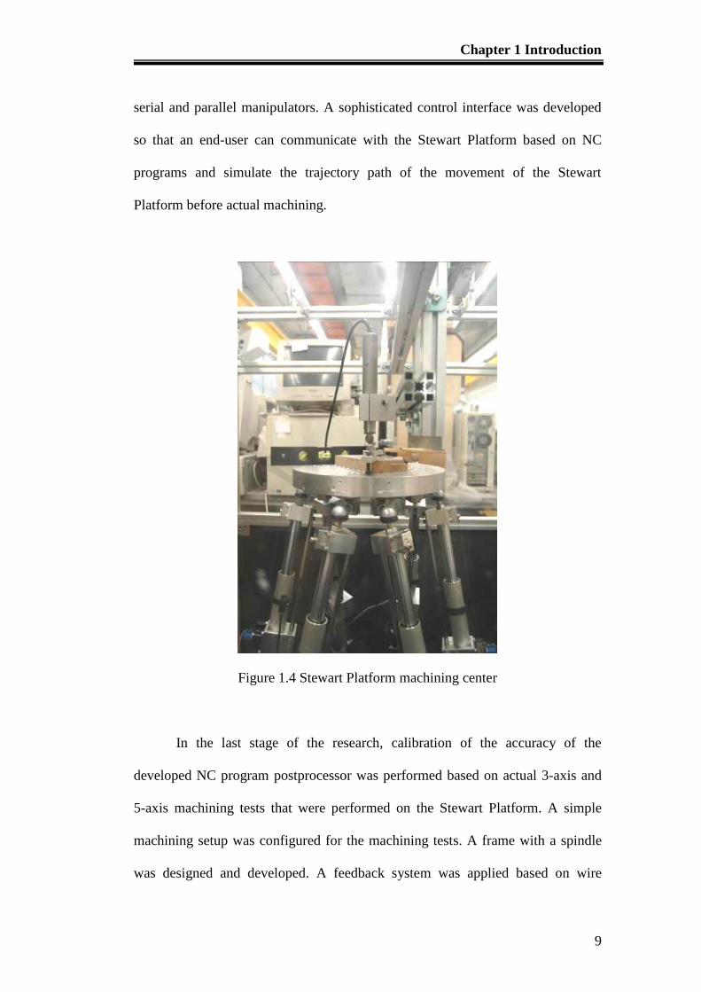
Currently, a Stewart Platform has been fabricated and assembled as shown
in Figure 1.4. A simple control system was developed to manipulate the platform
with a reasonable accuracy. The control interface software was developed such
that the end-user is able to communicate with the Stewart Platform through the
most common machining language, namely the NC programs. Automatic
conversion of NC programs from a commercial CAM package based on a CAD
model has been developed to control and manipulate the Stewart Platform to
achieve the machining purposes. Moreover, verification of the accuracy of the
software to convert the NC programs to the trajectory path of the Stewart Platform
has been carried out by implementing a feedback system.
In this research, the tasks completed are as follows. Firstly, the workspace
of the Stewart Platform was verified through performing simulations in
MATLAB® to determine and evaluate the limitations of the machining
dimensions. Literature review was performed to gain an understanding of the
kinematics and dynamics of the Stewart Platform as well as NC codes
programming, and to study the differences in the NC program control between
Chapter 1 Introduction
9
serial and parallel manipulators. A sophisticated control interface was developed
so that an end-user can communicate with the Stewart Platform based on NC
programs and simulate the trajectory path of the movement of the Stewart
Platform before actual machining.
Figure 1.4 Stewart Platform machining center
In the last stage of the research, calibration of the accuracy of the
developed NC program postprocessor was performed based on actual 3-axis and
5-axis machining tests that were performed on the Stewart Platform. A simple
machining setup was configured for the machining tests. A frame with a spindle
was designed and developed. A feedback system was applied based on wire
Chapter 1 Introduction
10
sensors that are mounted linearly on the actuators of the Stewart Platform, so that
the position and orientation of the end-effectors can be calibrated based on the
feedback of the links of the Stewart Platform. Experimental data was collected
during the machining tests. The data was analyzed and improvement was done on
the configuration of the system.
The six-leg manipulator suffers from the disadvantages of the complex
solution of direct kinematics, coupled problems of the position and orientation
movement. Thus, further research is performed after investigation on the
development of the PKM by reducing the 6-DOFs to 3-DOFs PKMs. The
reduction of the DOF of the PKMs has advantages in workspace and cost
reduction. However, the 3-DOF Parallel Kinematics Platform provides less
rigidity and DOF. Recently, Tsai [Tsai, 1996] has introduced a novel 3-DOF
translational platform that is made up of only revolute joints. The platform
performs pure translational motion and has a closed-form solution for the direct
and inverse kinematics. Hence, in terms of cost and complexity, 3-DOF 3-legged
Micro Parallel Kinematic Manipulator is cost effective and the kinematics of the
mechanism is further simplified for the purpose of control. However, the design
algorithms either do not exist or are very complicated.
To further increase the flexibility and functionality of the self-fabricated
Micro Stewart Platform, the concept of modular methodology is introduced. It
helps to optimize the performance of the 3-leg 3 DOF Parallel Manipulator and
the self-repair ability. Modular robots consist of many autonomous units or

Chapter 1 Introduction
11
modules that can be reconfigured into a huge number of designs. Ideally, the
modules will be uniform, and self-contained. The robot can be changed from one
configuration to another manually or automatically.
In short the major contributions of the author in his thesis are shown as
below. Further elaboration will be elaborated in the following chapters of the
thesis:
1. The development of a “post-processor”, or software routines, required to
translate the motion codes in standard-format NC part programs into the
required command joint coordinates for the control of Stewart Platform
used for 3D machining. This involves detailed understanding of coordinate
transformations, and transforming the required tool path, in NC part
program coordinates to the required joint coordinates for the Stewart
Platform. As part of the development of the post-processor, the workspace
of the Stewart Platform used was determined and the correct performance
of the post-processor demonstrated by actual machining on the Stewart
Platform. The accuracy of the motion achieved through measurement of
the actual lengths of the extensible legs of the Stewart Platform by
attaching external wire position sensors to each leg. This is because the
actuator of the Stewart Platform is belt driven by Stepper motor in open
loop. Even though there is encoder count read by the controller card, it
doesn’t reflect the actual length of the actuators. Hence the wire sensor can
be applied as the online position feedback system for the actual length of
Chapter 1 Introduction
12
the actuator. By using Newton-Raphson numerical method one is able to
calculate the actual position of the moving platform.
2. The extension of the post-processor for 5D or 5-axis machining which
involves significantly higher complexity. The correct performance of the
post-processor was demonstrated by actual machining of the part on the
platform.
3. The design and fabrication of a 3-DOF parallel manipulator intended for
“micro-machining”. The proper working if this manipulator together with
its own post-processor was also demonstrated
Chapter 2 Kinematics of Stewart Platform
13
Chapter 2 Kinematics of Stewart Platform
2.1 Introduction
Kinematics is the study of motion. The study of kinematics analyses the
motion of an object without considering the forces that cause the motion [Yee
1993]. Hence, only the position, velocity, acceleration and all the higher order
derivatives of the position variables are considered. The kinematics of rigid
mechanisms depends on the configuration of the joints.
Forward kinematics involves the calculation of the position and orientation
of the end-effector from the joint positions. In short, forward kinematics is a
mapping of the vectors of the joint coordinates to the vectors that indicate the
position and orientation of the end-effector. The forward kinematics of a Stewart
Platform is a complicated problem. The solution of the forward kinematics of
Stewart Platforms is usually only possible with numerical techniques.
On the other hand, inverse kinematics is the reverse of the forward
kinematics. It is the mapping of the possible sets of joint coordinates given the
orientation and position. The inverse kinematics of a Stewart Platform is typically
straightforward and simple. Comparatively, the solution of the inverse kinematics
of a serial manipulator is more complicated.
As shown in Figure 2.1, the position and orientation of the mobile
platform of the Gough-Stewart Platform are controlled by changes in the six links
Chapter 2 Kinematics of Stewart Platform
14
li, which are connected in parallel between the mobile platform of diameter of 30
cm and the base with diameter of 60 cm. The six base attachment joints are
universal joints and all the platform attachment joints are spherical joints. The
joints at the base are universal joints because only two DOFs are needed, which
are the rotation freedom about, and the rotational freedom to make an angle with
the respective base sides. The spherical joints are used because extra DOFs are
needed so that each link can rotate by itself.
Link l1
Zp
Xp
Yp
ZB
YB
XB
30o
90o
30o
B1
B2
B3
B4
B5
B6
P1
P2
P3
P4
P5
P6
Link l2
Link l3
Link l4Link l
5
Link l6
Mobile Platform
Fixed Base
Spherical Joint
Universal Joint
Figure 2.1 The Gough-Stewart Platform
Chapter 2 Kinematics of Stewart Platform
15
The mobile platform and the base are split into six individual joints, which
are allocated 15˚ symmetrically on both sides of each 120˚ line of the platform.
The symmetrical allocation of the joints is to ensure more uniform loads
distribution on the base and the platform. Each pair of adjacent platform joints pi
with 30˚ difference forms a triangle-like quadrilateral with two adjacent base
joints bi of 90˚ difference, such as p1 and p6 to b1 and b6, as shown in Figure 2.1.
The sides of the triangles are links of the platform. All the joints form
inverted and forward triangles. The formation of the triangular shape strengthens
the force to hold the load of the platform and the workpiece.
2.2 Inverse kinematics
The inverse kinematics problem is almost trivial for the Stewart Platform
and is extensively used in many methods.
First, the Stewart Platform kinematics can be illustrated in many ways but
the most common set of parameters includes the minimal and maximal link
lengths ( ), the radii of the platform and the base, the joint placement is
determined as the angle between the closest joints for both the platform and the
base, and the joint moving volume. Based on these common sets of parameters,
iB
and iP
as shown in Equation (2.1) can be calculated. Inverse kinematics can
be described with Equations (2.1) and (2.2).
, (2.1)
minmax, ii
ii pRtP
Chapter 2 Kinematics of Stewart Platform
16
6
(2.2)
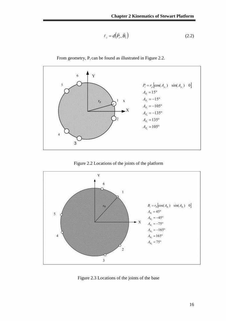
From geometry, Pi can be found as illustrated in Figure 2.2.
Figure 2.2 Locations of the joints of the platform
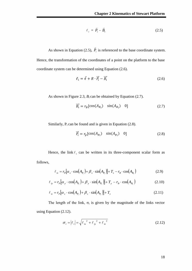
Figure 2.3 Locations of the joints of the base
iii BPd
,
Y

Chapter 2 Kinematics of Stewart Platform
17
As shown in Figures 2.2 and 2.3, a coordinate system is defined for the
base and the platform respectively. Each of the six points on the base is described
by a position vector, , which is defined with respect to the base coordinate
system. Similarly, each of the six points on the platform is described by a position
vector, , with respect to the platform coordinate system. The left superscript P
denotes that the vector is referenced to the platform coordinate system while the
superscript B denotes reference to the base coordinate system. This notation will
be used in the following derivation of the inverse kinematics.
The matrix R shown in Equation (2.1) can be written in another form as
shown in Equation (2.3) [Soh et al, 2002]:
(2.3)
Conversely, the orientation of the base with respect to the platform, PR, is
given by,
PR = R
-1 = R
T= (2.4)
Having defined the position and orientation of the platform with respect to
the base, the links i are defined in Equation (2.5), which are the vectors of the ith
links from Bi to Pi vector algebra.
zzz
yyy
xxx
R
zyx
zyx
zyx
Chapter 2 Kinematics of Stewart Platform
18
= - (2.5)
As shown in Equation (2.5), is referenced to the base coordinate system.
Hence, the transformation of the coordinates of a point on the platform to the base
coordinate system can be determined using Equation (2.6).
(2.6)
As shown in Figure 2.3, Bi can be obtained by Equation (2.7).
[
] (2.7)
Similarly, Pi can be found and is given in Equation (2.8).
[
] (2.8)
Hence, the link can be written in its three-component scalar form as
follows,
iii BBxPxPxPix ArTAAr cossincos (2.9)
iii BByPyPyPiy ArTAAr cossincos (2.10)
zPzPzPiz TAArii sincos (2.11)
The length of the link, σi is given by the magnitude of the links vector
using Equation (2.12).
222
iziyixii (2.12)
i iP
iB
iP
i

Chapter 2 Kinematics of Stewart Platform
19
2.3 Forward kinematics
The forward kinematics for a Stewart Platform can be mathematically
formulated in several ways. Every representation of the problem has its
advantages and disadvantages, when a different optimization algorithm is applied
[Jakobovic and Jelenkovic, 2002].
The configuration of the actual Stewart Platform has to be represented in
order to define a forward kinematics problem [Jakobovic and Jelenkovic, 2002],
i.e., the actual position and orientation of the mobile platform have to be
represented. The most commonly used approach utilizes the three positional
coordinates of the center of the mobile platform and the three angles that define its
orientation. The coordinates are represented by the vector:
z
y
x
t
t
t
t
(2.13)
The three rotational angles are defined as the roll γ, pitch β and yaw angles
α. The values of the angles represent the consecutive rotations about the X-, Y-
and Z-axes respectively. From Figure 2.1, the Stewart Platform is defined with six
vectors for the base and six vectors for the mobile platform, which define the six
joint coordinates on each platform.
0
iy
ix
i B
B
B
,
0
iy
ix
i P
P
P
, i = 1, …., 6 (2.14)(2.15)

Chapter 2 Kinematics of Stewart Platform
20
These vectors and Pi shown in Figure 2.1 are constant values with
respect to the local coordinate systems of the base XBYBZB and the local
coordinate systems of the mobile platform XPYPZP. The base and the mobile
platform are assumed to be planar; therefore, it can be perceived that the Z-
coordinate of the joint coordinate, Bi and Pi is zero. The link vector can be
expressed as Equation (2.16) [Jakobovic and Jelenkovic, 2002].
iii PRtBl
, i = 1 ... 6 (2.16)
R is the rotational matrix that can be determined from the three rotational
angles. The orientation of the mobile platform is rotated with respect to the mobile
platform coordinate frame. In this research, the coordinate frame rotates about the
reference X-axis (roll) by γ, followed by a rotation about the reference Y-axis
(pitch) by an angle β before a rotation about the reference Z-axis (yaw) by an
angle α. The resultant Eularian rotation is derived as below [Craig, 1986].
,,,),,( XYZXYZ RRRR
cs
sc
cs
sc
cs
sc
0
0
001
0
010
0
100
0
0
ccscs
sccssccssscs
sscsccsssccc
(2.17)
where sin
cos
s
c
Chapter 2 Kinematics of Stewart Platform
21
If the position and orientation of the mobile platform are known, the length
of each link can be determined according to Equation (2.18).
iii pRtbD
, , i = 1, 2,…, 6 (2.18)
D represents the Euclidean distance between the two vectors. For an
arbitrary solution to a forward kinematics problem, i.e., an arbitrary position and
orientation of the mobile platform, the error can be expressed as the sum of the
squares of the differences between the calculated and the actual length values.
Having stated the above relations, one can define the first optimization function
and the related unknowns as
26
1
22
1 ,
i
iii pRtbDF
(2.19)
Tzyx tttX 1
(2.20)
where is the first optimization function, and are the translation and
orientation parameters of the platform
The forward kinematics of a Stewart Platform determines the pose of the
platform with respect to its base given the actuators lengths. The pose of the
platform can be defined by Equation (2.21) as shown below:
ii
B PTP (2.21)
where
10 31
1333 rTRotT .
Chapter 2 Kinematics of Stewart Platform
22
T is the corresponding 4×4 homogeneous coordinate matrix. It consists of
a 3×3 rotational matrix, 33Rot which is defined by the rotational motions about
the X-axis, Y-axis and Z-axis with respect to the platform coordinate system, and
the translational matrix 13rT which is defined by the translational motions along
the X-axis, Y-axis and Z-axis with respect to the base coordinate system.
coscossincossin
sincoscossinsincoscossinsinsincossin
sinsincossincoscossinsinsincoscoscos
33Rot
(2.22)
Z
Y
x
xr
T
T
T
T 13 (2.23)
The homogeneous translational matrix contains redundant information
because its 4×4 elements can be solved uniquely from the six parameters that
control the six DOFs, which are the three rotational parameters roll-pitch-yaw ,
and , and the three translation parameters Tx, Ty and Tz. These six parameters
can be presented as Equation (2.24).
Tzyx TTTq (2.24)
zi
yi
xi
iii
S
S
S
BPqTqS
)()( (2.25)
iziyixii lSSSSG 222
)( where i = 1, 2, 3,…, 6 (2.26)

Chapter 2 Kinematics of Stewart Platform
23
Equations (2.25) and (2.26) define function (G:ql); since G(Si) cannot
be inverted in a closed form, vector S can be estimated by linear function G(S(q))
around initial value of the actuator length l, with respect to vector q, using
Newton’s method [Jakobovic and Jelen 2002].
i
ii
ii
i
i ldq
dGqq
dq
dGlllq
dq
dGll
ii
1
00 (2.27)
i
i
i
ii
i
ii
i
ii Pdq
dT
ds
dGBPqT
dq
d
ds
dG
dq
ds
ds
dG
dq
dG (2.28)
1
1
2
2
1
2
2
1
2
2
1
)(
)(
)(
1
222
222
222
222
222
222
222
zi
iy
xi
ziyixi
ziyixi
zi
ziyixi
yi
ziyixi
xi
z
ziyixi
y
ziyixi
x
ziyixi
z
y
x
i
S
S
S
SSS
SSS
S
SSS
S
SSS
S
dS
SSSd
dS
SSSd
dS
SSSd
dS
dG
dS
dG
dS
dG
ds
dG
(2.29)
Besides, dR/dq has to be defined. Since T is a 2-dimensional matrix, and q
is a 1-dimensional vector, the derivative will be 3-dimentional. The first derivative
is the derivative of the transformation matrix with respect to the first element of
the vector q, dR/dq, the second is dR/dq2, and so forth. The pose of the platform
coordinate system {P} can be obtained based on the following sequence of
fundamental rotations and translations about the base coordinate system {B}.
The resulting homogeneous transformation matrix is of the following form:
Chapter 2 Kinematics of Stewart Platform
24
1000
coscossincossin
sincoscossinsincoscossinsinsincossin
sinsincossincoscossinsinsincoscoscos
Z
Y
X
T
T
T
T
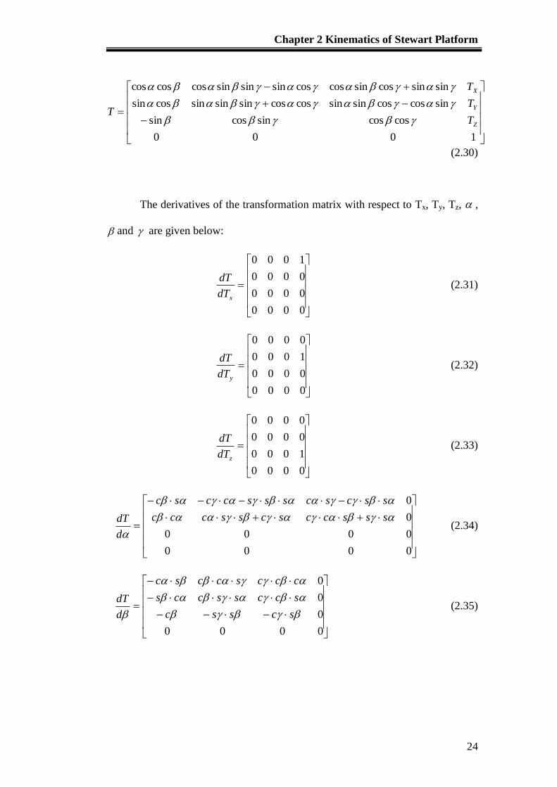
(2.30)
The derivatives of the transformation matrix with respect to Tx, Ty, Tz, ,
and are given below:
(2.31)
(2.32)
(2.33)
0000
0000
0
0
sssccscssccc
sscscsssccsc
d
dT (2.34)
0000
0
0
0
scssc
sccssccs
cccsccsc
d
dT (2.35)
0000
0000
0000
1000
xdT
dT
0000
0000
1000
0000
ydT
dT
0000
1000
0000
0000
zdT
dT
Chapter 2 Kinematics of Stewart Platform
25
0000
00
00
00
cscc
sssccsscsc
sscscssscc
d
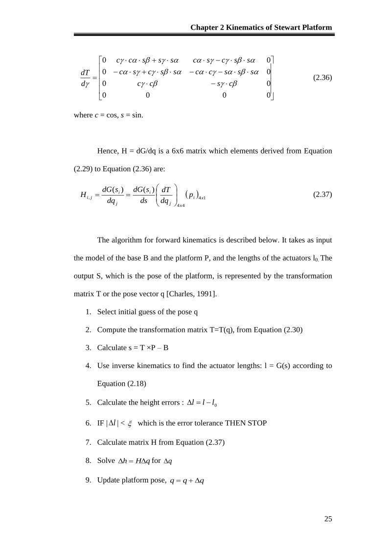
dT (2.36)
where c = cos, s = sin.
Hence, H = dG/dq is a 6x6 matrix which elements derived from Equation
(2.29) to Equation (2.36) are:
14
44
,
)()(xi
xj
i
j
i
ji pdq
dT
ds
sdG
dq
sdGH
(2.37)
The algorithm for forward kinematics is described below. It takes as input
the model of the base B and the platform P, and the lengths of the actuators l0. The
output S, which is the pose of the platform, is represented by the transformation
matrix T or the pose vector q [Charles, 1991].
1. Select initial guess of the pose q
2. Compute the transformation matrix T=T(q), from Equation (2.30)
3. Calculate s = T ×P – B
4. Use inverse kinematics to find the actuator lengths: l = G(s) according to
Equation (2.18)
5. Calculate the height errors : 0lll
6. IF | l | < which is the error tolerance THEN STOP
7. Calculate matrix H from Equation (2.37)
8. Solve qHh for q
9. Update platform pose, qqq
Chapter 2 Kinematics of Stewart Platform
26
10. GOTO step 2.
The forward kinematics algorithm performs iterations and calculates the
increment in the platform pose and the link lengths for the new pose h. It
terminates when the difference between the calculated and the desired actuator
values drops below a predetermined iteration error, ξ. Step 8 involves an inversion
of the matrix H. If the matrix is near singularity, it means the position is close to
the singular position and special attention is necessary.
Equation (2.27) gives the relationship between the infinitesimal changes of
actuator lengths and the changes in pose. Dividing both sides of this equation by
an infinitesimal time period gives a relationship between the actuator velocities
and the translational and rotational velocities of the platform. The inverse of
matrix H is also called the Jacobian matrix.
1 HJ (2.38)
hJq (2.39)
In this method, all the joints of the platform or actuators on the base need
not be in one plane. This is a useful fact when the joint coordinates are estimated
after the manipulator has been manufactured, and newly re-calibrated values are
used for the forward kinematics analysis. However, it is important to note that the
solution for forward kinematics analysis is not unique. The actuator lengths
feedback is not necessarily reliable when the feature space feedback is used and
the approximate positions of the actuators are known. However, if the manipulator
Chapter 2 Kinematics of Stewart Platform
27
enters a singular position, the pose of the platform cannot be calculated with
confidence from the actuator lengths.
2.4 Workspace
In general, the workspace of a Stewart Platform is the set of all pairs of
position and orientation that the end-effector can reach. In short, the workspace is
the space for which a kinematics solution exists. One of the difficulties in
representing the workspace is that the workspace is described with the parameters
of X, Y, Z, Roll, Pitch and Yaw. It is very difficult to be presented graphically. By
making reference to the work of Bonev and Ryu [1999], the discretization method
is applied for the computation of the workspace of a 6-DOF Stewart Platform.
For a Stewart Platform, the usable workspace is a subset of the reachable
and dexterous workspace. The reachable workspace, taking into consideration the
limits of the actuators, is the set of all the points an end-effector can reach for at
least one orientation. A dexterous workspace is the set of all points that the end-
effector can reach for an arbitrary orientation. Besides these workspaces, a
workspace can also be defined as the directed workspace consisting of all the
points an end-effector can reach for one given orientation, and the usable
workspace is a connected portion of the workspace that does not contain
singularities.
Chapter 2 Kinematics of Stewart Platform
28
The main subset of the complete workspace that is defined in the 3-D
rotation space is the orientation workspace. The 3-D orientation workspace is
probably the most difficult workspace to determine and represent. However, as a
six-DOF Stewart Platform is mainly used for 5-axis machining operations, only
the set of all the attainable directions of the approach vector of the mobile
platform are of interest, which is the unit vector along the axi-symmetric platform.
This 2-D workspace is defined as the projected orientation workspace.
Using the discretization method, the 2-D subset of the orientation
workspace of the Gough-Stewart Platform is calculated using MATLAB®. The
possible directions of the approach vector are represented as the inside of a
general conical surface. Furthermore, in the case of an axi-symmetric Gough-
Stewart Platform, a close approximation of the projected orientation workspace
can be found directly by fixing one of the modified Euler angles and finding an
intersection of the orientation workspace.
To implement the 2-D discretization method for the calculation of the
projected workspace, a few basic kinematics constraints that limit the workspace
are considered. As shown in Figure 2.1, the base universal joints are denoted by Bi
and the mobile platform spherical joints by Pi (I = 1, 2, … 6). Let the orientation
of the mobile platform be represented by the rotation matrix R. Hence, by
knowing the given position and orientation of the mobile platform, the length of
each link can be calculated using the inverse kinematics methods as shown in
Equation (2.40).
Chapter 2 Kinematics of Stewart Platform
29
iii pRtbl
, i = 1, …. 6 (2.40)
Instead of the inverse kinematics analysis, three main mechanical
constraints that limit the workspace of a Gough-Stewart Platform would need to
be considered in the determination of the workspace. These three constraints are
presented as below:
The stroke of the actuators
The limited stroke of an actuator imposes a length constraint on link i,
such that max,min, iii , for i = 1, 2,….. 6 where min,i and max,i are the
minimum and maximum lengths of the link i respectively.
The range of the passive joints
Each passive joint has a limited range of angular motions due to the
characteristics of commercially available joints. Let jAi be the unit vector with
respect to the base frame along the axis of symmetry of the universal joint at point
Ai. Let the maximum misalignment angle of the universal joint be i . Let the unit
vector along link i be denoted byi
ii
i
BAn
. Hence, the limit on the base joint i
imposes a constraint, such that
.62,1cos 1 forinj ii
T
Ai
(2.41)
Similarly,
.62,1cos 1 forinj ii
T
Bi
(2.42)
Chapter 2 Kinematics of Stewart Platform
30
where, '
Bij is the unit vector with respect to the mobile frame that is along the axis
of symmetry of the spherical joint at point Bi. i is the maximum misalignment
angle of the spherical joint.
To simplify the calculation, a geometric model is implemented as a
constraint where AB is the height difference of the center platform to the center of
the base and i is the length of the links. Hence, the formula can be derived as
follows.
.6,2,1sin 1
foril
ABi
i
for the universal joints (2.43)
.6,2,1cos 1
foril
ABi
i
for the spherical joints (2.44)
The link interference
The links can be approximated by a cylinder of diameter D. This imposes
a constraint on the relative position of the pairs of links, such that the distance
between the two centers of the actuator must be larger than the diameter of the
cylinder of the actuator.
DBABAcedis jjii ,tan for I = 1, 2,…6 (2.45)
Hence, the minimum distance between every two line segments
corresponding to the links of the Stewart Platform should be greater than or equal
to D.
Chapter 2 Kinematics of Stewart Platform
31
2.5 Algorithm for workspace discretization calculation
The simulation is performed by applying all the mechanical kinematics
constraints using MATLAB®. The first requirement sets for the Euler angles are
defined by rotating the mobile frame about the base Z-axis by an angle, about the
mobile Y-axis by an angle, and finally about the mobile X-axis by an angle.
Hence, the rotation matrix can be defined as below:
,,,),,( XYZXYZ RRRR (2.46)
Based on the characteristics of the passive joints in the assembly, the
maximum misalignment angle of the spherical joint is set as i = 20˚ and the
maximum misalignment angle of the universal joint is set as i = 45˚. It has been
observed that the main constraint that is violated is usually the range of the
platform joints. In fact, the link interference is never encountered. Hence, to
reduce computation time, the interference check can be disabled. The result of the
MATLAB® simulation to calculate the workspace is shown in Figure 2.4.
Chapter 2 Kinematics of Stewart Platform
32
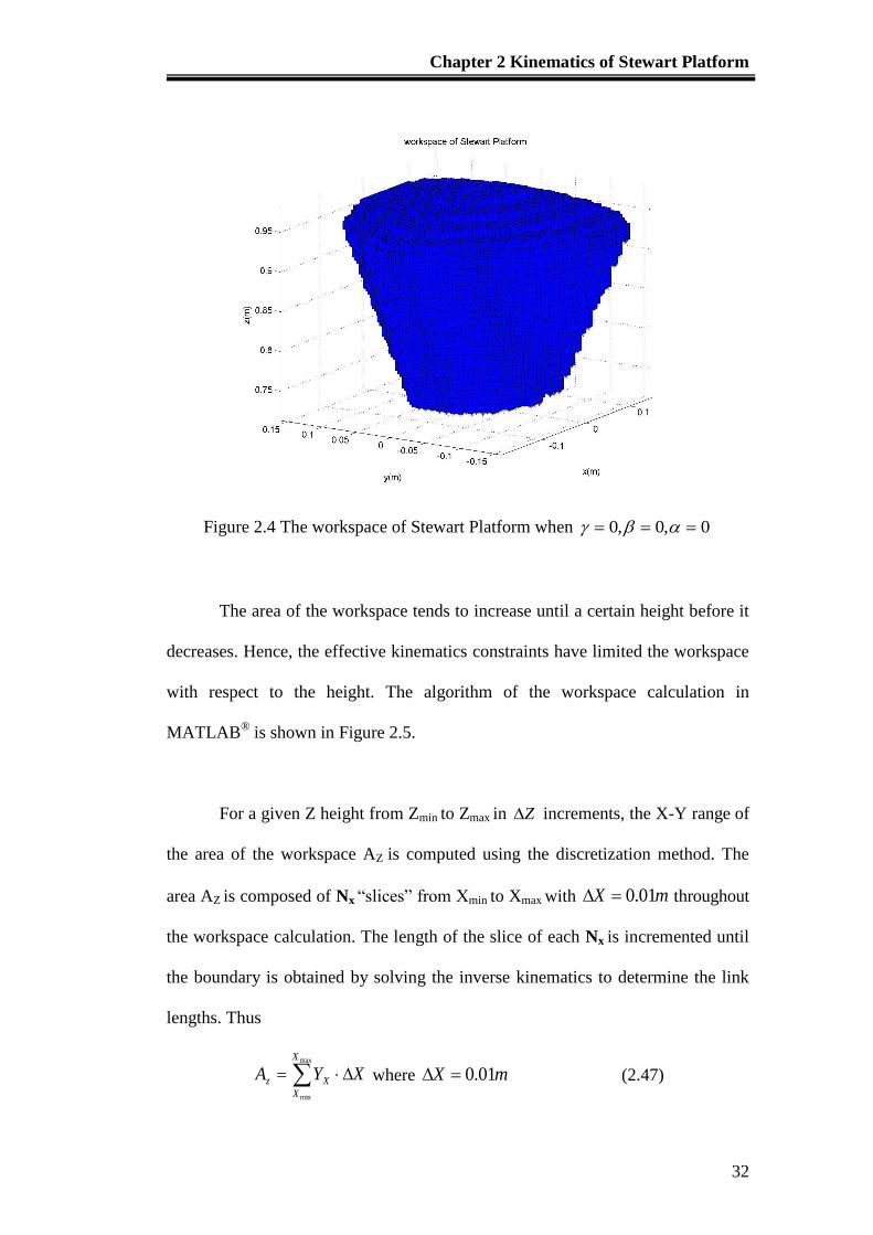
Figure 2.4 The workspace of Stewart Platform when
The area of the workspace tends to increase until a certain height before it
decreases. Hence, the effective kinematics constraints have limited the workspace
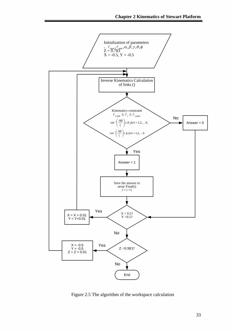
with respect to the height. The algorithm of the workspace calculation in
MATLAB® is shown in Figure 2.5.
For a given Z height from Zmin to Zmax in Z increments, the X-Y range of
the area of the workspace AZ is computed using the discretization method. The
area AZ is composed of Nx “slices” from Xmin to Xmax with mX 01.0 throughout
the workspace calculation. The length of the slice of each Nx is incremented until
the boundary is obtained by solving the inverse kinematics to determine the link
lengths. Thus
max
min
X
X
Xz XYA where mX 01.0 (2.47)
0,0,0
Chapter 2 Kinematics of Stewart Platform
33
Initialization of parameters,Z = 0.783X = -0.5, Y = -0.5
,,,,,, minmax
Inverse Kinematics Calculationof links ()
Kinematics constraint
max,min, iii
.6,2,1sin 1
foril
ABi
i
.6,2,1cos 1
foril
ABi
i
Answer = 1
Answer = 0
Save the answer toarray Final(i)
i = i +1
X < 0.5?Y <0.5?
Z <0.983?
X = X + 0.01Y = Y+0.01
X = -0.5Y = -0.5
Z = Z + 0.01
End
No
Yes
Yes
No
Yes
No
Figure 2.5 The algorithm of the workspace calculation
Chapter 2 Kinematics of Stewart Platform
34
The total volume V is calculated as the sum of the incremental volumes of
ZAz .
Thus max
min
Z
Z
z ZAV where mZ 01.0 (2.48)
The calculation of the area of the workspace is performed by setting
0,0,0 and the Z-increments as 0.01m. Using the volume calculation
method, the volume of the workspace can be obtained. The total volume of the
workspace is 12179 cm3 or 0.012179 m
3.
After obtaining the result of the workspace in Figure 2.5, the limitation of
the position and orientation of the Stewart Platform can be verified. Hence, the
motion of the platform can be operated safely within the allowance of the
workspace. As a result, singularities can be avoided and the possible damage to
the passive joints can be minimized.
Chapter 2 Kinematics of Stewart Platform
35
2.6 Singular Position
The singularity configurations of a Stewart Platform introduce one or more
extra DOF to the system. These additional DOFs are independent of the
instantaneous velocities of the actuators and hence cannot be controlled by the
motion of the links. This type of situation happens when there is no inverse
solution for the Jacobian matrix, which occurs when the determinant of the matrix
is equal to zero. Hence, if a linear transformation relating the velocity of the joint
to the Cartesian velocity of mobile platform can be inverted for the calculation the
joint velocity of actuator with a given Cartesian velocity [Craig, 1986], the matrix
is non-singular.
As mentioned previously, the determinant for the inverse Jacobian is too
complex to be solved. Hence, the effects of the singularities can only be felt when
the control is performed using the dynamics equations and the Jacobian. Since
both equations are not used, it would not be easy to identify these singularity
problems [Yee, 1993].
All manipulators have singularities at the boundary of their workspaces,
and most have loci of singularities inside their workspaces. Singularities are
normally classified into two categories:
1. Workspace boundary singularities are those that happen when the platform
is fully stretched out or folded back on itself such that the end-effector is
near or at the boundary of the workspace.
Chapter 2 Kinematics of Stewart Platform
36
2. Workspace interior singularities are those that occur away from the
workspace boundary and are generally caused by two or more joints axes
lining up.
Based on this classification of the singularities, for the particular Stewart
Platform in this research, two kinds of singularity configurations have been
identified according to the work of Fichter [1986].
The first type of singularity configurations can be observed from the
physical structure of the Stewart Platform. When the plane of the surface of the
mobile platform is parallel to any one of the planes of the links as shown in Figure
2.6, uncertainty exists due to the changes in the motion of the links to manipulate
the end-effectors of the platform. Since the spherical joint acts as a pivot between
the two surfaces of mobile platform and the respective link, the new corner
between the surfaces at the new position could either point inwards or outwards,
as shown in the Type 1 configuration of Figure 2.6.
The second type of singularity configurations is not easily observable.
When the mobile platform is oriented at 90˚ either clockwise or anticlockwise
about the Z-axis (Yaw), without any angular rotation about the X-axis (Roll) and
the Y-axis (Pitch) as shown in Figure 2.6, Type 2 singularity happens when the
mobile platform is parallel to the base. All the tangents of the spherical joints are
perpendicular to the respective edge of the base. Thus, all the loci of the points at
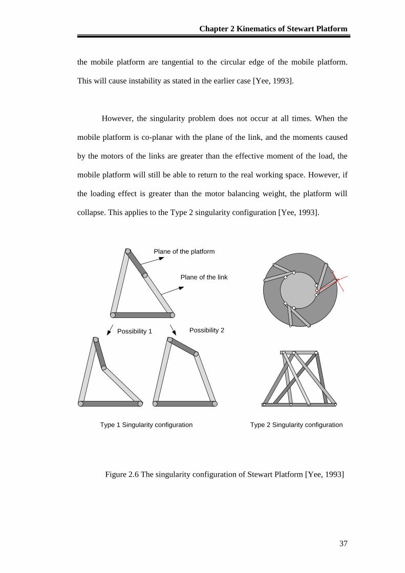
Chapter 2 Kinematics of Stewart Platform
37
the mobile platform are tangential to the circular edge of the mobile platform.
This will cause instability as stated in the earlier case [Yee, 1993].
However, the singularity problem does not occur at all times. When the
mobile platform is co-planar with the plane of the link, and the moments caused
by the motors of the links are greater than the effective moment of the load, the
mobile platform will still be able to return to the real working space. However, if
the loading effect is greater than the motor balancing weight, the platform will
collapse. This applies to the Type 2 singularity configuration [Yee, 1993].
Type 1 Singularity configuration Type 2 Singularity configuration
Possibility 1 Possibility 2
Plane of the platform
Plane of the link
Figure 2.6 The singularity configuration of Stewart Platform [Yee, 1993]
Chapter 2 Kinematics of Stewart Platform
38
During the normal operation of a Stewart Platform, the singularity
configurations should always be prevented to reduce the risk of uncertainty in the
position and orientation, as well as to prevent overloading of the joints of the
platform. Precautionary steps are taken through both the hardware and software
aspects. A MATLAB® program has been developed to verify the singularity
points by restricting the boundary of the movement through limiting the maximum
rotation of the Z-axis to and the angle between the spherical joints and the
platform to be less than . Furthermore, the angular rotation between the
universal joints and the base is restricted to , which all are below the limits
of the singularity configuration. Next, hardware precaution can be applied by
installing a magnetic sensor to limit the movements of the links physically to
prevent any possibility for singularity to occur due to the over traveling of the
links.
60
20
45
Chapter 3 Fundamentals of Machining
39
Chapter 3 Fundamentals of Machining
3.1 Introduction
Computer Numerical Control (CNC) is a methodology of communicating
with the machining centers through G-codes and M-codes instructions for
manipulating the machine tool or workpiece. CNC performs according to
numerically directed interpolation of the tool path of the cutting tool in the
workspace of the machine center. The parameters of the CNC operations can be
modified through the software within the controller.
The fundamental of CNC control is to move the machine tool along a path
from one point to another. Certain machines can only perform planar motions,
such as contouring along the X-axis and Y-axis while the Z-axis is controlled
separately. In certain machines, additional two axes of rotation are implemented to
control the orientation of the cutter or workpiece during the machining process.
This can be achieved simultaneously along with the translation motion in the
Cartesian workspace.
In modern manufacturing, 4-axis and 5-axis machines are becoming more
popular due to their flexibility and capability to machine complex workpieces.
Hence, a 3-axis machine can be used to move the tool head in the X, Y and Z-
directions while the additional axes allow the workpieces to be rotated about the
X-axis and Y-axis, similar to a lathe. These rotational axes are also called the A-
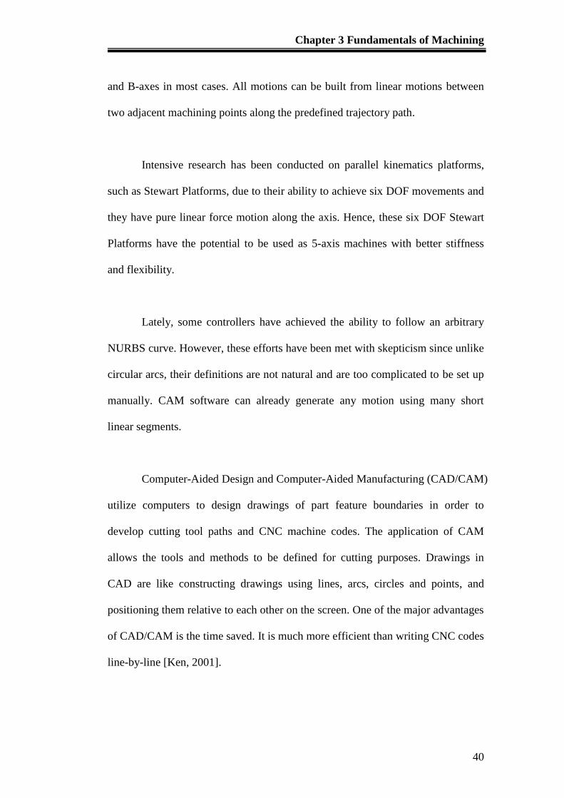
Chapter 3 Fundamentals of Machining
40
and B-axes in most cases. All motions can be built from linear motions between
two adjacent machining points along the predefined trajectory path.
Intensive research has been conducted on parallel kinematics platforms,
such as Stewart Platforms, due to their ability to achieve six DOF movements and
they have pure linear force motion along the axis. Hence, these six DOF Stewart
Platforms have the potential to be used as 5-axis machines with better stiffness
and flexibility.
Lately, some controllers have achieved the ability to follow an arbitrary
NURBS curve. However, these efforts have been met with skepticism since unlike
circular arcs, their definitions are not natural and are too complicated to be set up
manually. CAM software can already generate any motion using many short
linear segments.
Computer-Aided Design and Computer-Aided Manufacturing (CAD/CAM)
utilize computers to design drawings of part feature boundaries in order to
develop cutting tool paths and CNC machine codes. The application of CAM
allows the tools and methods to be defined for cutting purposes. Drawings in
CAD are like constructing drawings using lines, arcs, circles and points, and
positioning them relative to each other on the screen. One of the major advantages
of CAD/CAM is the time saved. It is much more efficient than writing CNC codes
line-by-line [Ken, 2001].
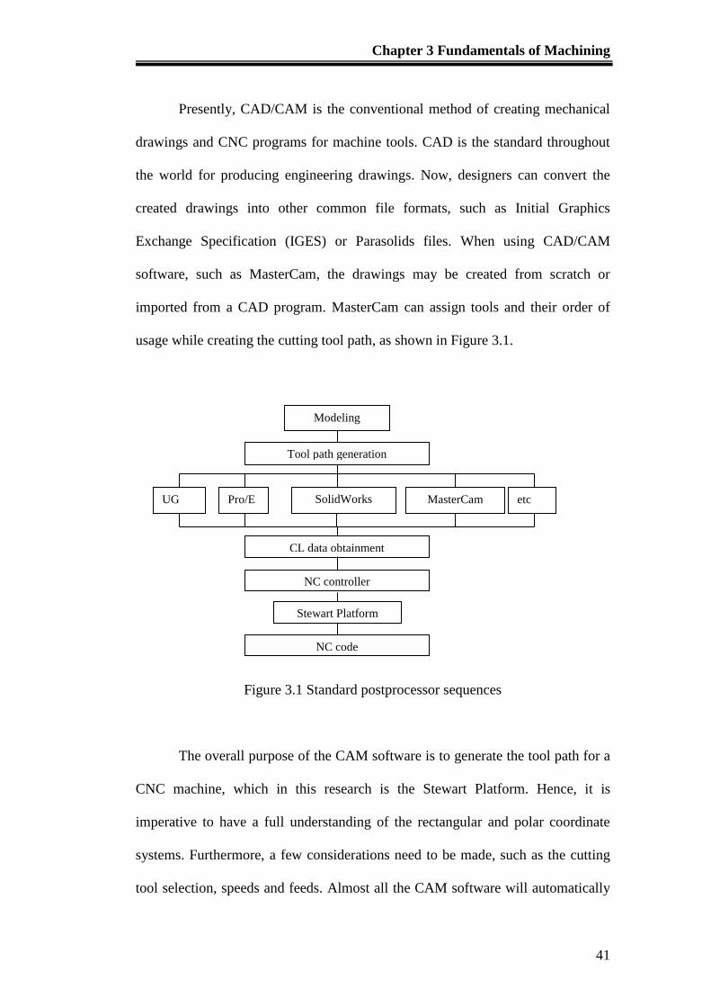
Chapter 3 Fundamentals of Machining
41
Presently, CAD/CAM is the conventional method of creating mechanical
drawings and CNC programs for machine tools. CAD is the standard throughout
the world for producing engineering drawings. Now, designers can convert the
created drawings into other common file formats, such as Initial Graphics
Exchange Specification (IGES) or Parasolids files. When using CAD/CAM
software, such as MasterCam, the drawings may be created from scratch or
imported from a CAD program. MasterCam can assign tools and their order of
usage while creating the cutting tool path, as shown in Figure 3.1.
Figure 3.1 Standard postprocessor sequences
The overall purpose of the CAM software is to generate the tool path for a
CNC machine, which in this research is the Stewart Platform. Hence, it is
imperative to have a full understanding of the rectangular and polar coordinate
systems. Furthermore, a few considerations need to be made, such as the cutting
tool selection, speeds and feeds. Almost all the CAM software will automatically
Modeling
Tool path generation
UG Pro/E SolidWorks MasterCam etc
CL data obtainment
NC controller
Stewart Platform
NC code
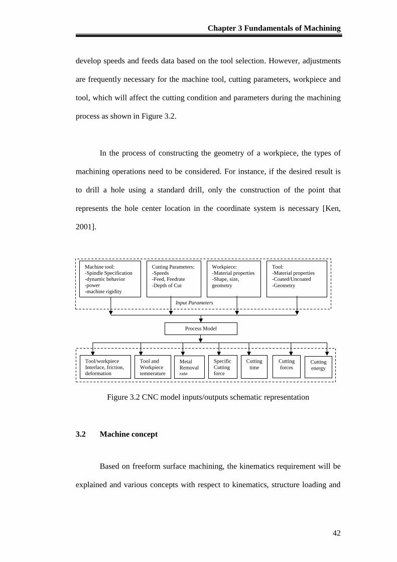
Chapter 3 Fundamentals of Machining
42
develop speeds and feeds data based on the tool selection. However, adjustments
are frequently necessary for the machine tool, cutting parameters, workpiece and
tool, which will affect the cutting condition and parameters during the machining
process as shown in Figure 3.2.
In the process of constructing the geometry of a workpiece, the types of
machining operations need to be considered. For instance, if the desired result is
to drill a hole using a standard drill, only the construction of the point that
represents the hole center location in the coordinate system is necessary [Ken,
2001].
Figure 3.2 CNC model inputs/outputs schematic representation
3.2 Machine concept
Based on freeform surface machining, the kinematics requirement will be
explained and various concepts with respect to kinematics, structure loading and
Machine tool:
-Spindle Specification -dynamic behavior
-power
-machine rigidity
Cutting Parameters:
-Speeds -Feed, Feedrate
-Depth of Cut
Workpiece:
-Material properties -Shape, size,
geometry
Tool:
-Material properties -Coated/Uncoated
-Geometry
Input Parameters
Process Model
Tool/workpiece
Interface, friction, deformation
Tool and
Workpiece temperature
Metal
Removal rate
Specific
Cutting force
Cutting
time
Cutting
forces Cutting
energy
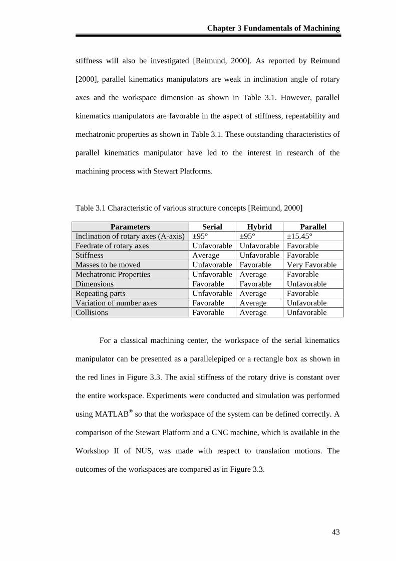
Chapter 3 Fundamentals of Machining
43
stiffness will also be investigated [Reimund, 2000]. As reported by Reimund
[2000], parallel kinematics manipulators are weak in inclination angle of rotary
axes and the workspace dimension as shown in Table 3.1. However, parallel
kinematics manipulators are favorable in the aspect of stiffness, repeatability and
mechatronic properties as shown in Table 3.1. These outstanding characteristics of
parallel kinematics manipulator have led to the interest in research of the
machining process with Stewart Platforms.
Table 3.1 Characteristic of various structure concepts [Reimund, 2000]
Parameters Serial Hybrid Parallel
Inclination of rotary axes (A-axis) ±95° ±95° ±15.45°
Feedrate of rotary axes Unfavorable Unfavorable Favorable
Stiffness Average Unfavorable Favorable
Masses to be moved Unfavorable Favorable Very Favorable
Mechatronic Properties Unfavorable Average Favorable
Dimensions Favorable Favorable Unfavorable
Repeating parts Unfavorable Average Favorable
Variation of number axes Favorable Average Unfavorable
Collisions Favorable Average Unfavorable
For a classical machining center, the workspace of the serial kinematics
manipulator can be presented as a parallelepiped or a rectangle box as shown in
the red lines in Figure 3.3. The axial stiffness of the rotary drive is constant over
the entire workspace. Experiments were conducted and simulation was performed
using MATLAB® so that the workspace of the system can be defined correctly. A
comparison of the Stewart Platform and a CNC machine, which is available in the
Workshop II of NUS, was made with respect to translation motions. The
outcomes of the workspaces are compared as in Figure 3.3.
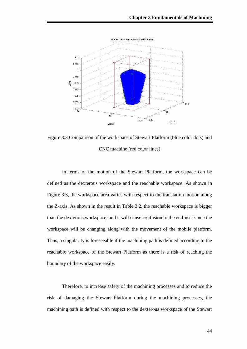
Chapter 3 Fundamentals of Machining
44
Figure 3.3 Comparison of the workspace of Stewart Platform (blue color dots) and
CNC machine (red color lines)
In terms of the motion of the Stewart Platform, the workspace can be
defined as the dexterous workspace and the reachable workspace. As shown in
Figure 3.3, the workspace area varies with respect to the translation motion along
the Z-axis. As shown in the result in Table 3.2, the reachable workspace is bigger
than the dexterous workspace, and it will cause confusion to the end-user since the
workspace will be changing along with the movement of the mobile platform.
Thus, a singularity is foreseeable if the machining path is defined according to the
reachable workspace of the Stewart Platform as there is a risk of reaching the
boundary of the workspace easily.
Therefore, to increase safety of the machining processes and to reduce the
risk of damaging the Stewart Platform during the machining processes, the
machining path is defined with respect to the dexterous workspace of the Stewart
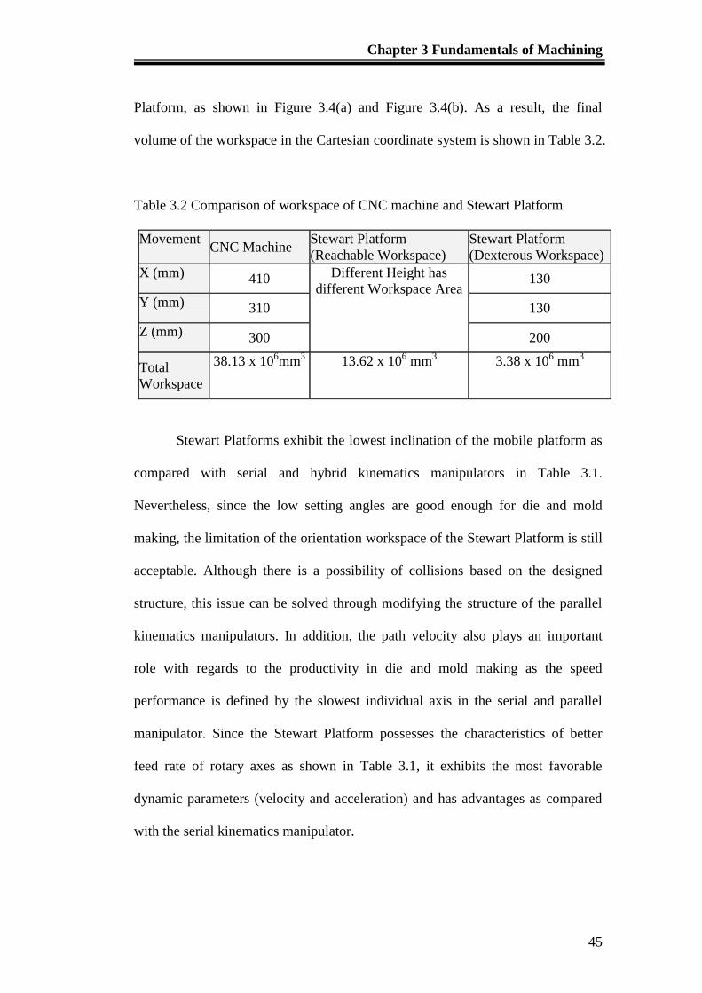
Chapter 3 Fundamentals of Machining
45
Platform, as shown in Figure 3.4(a) and Figure 3.4(b). As a result, the final
volume of the workspace in the Cartesian coordinate system is shown in Table 3.2.
Table 3.2 Comparison of workspace of CNC machine and Stewart Platform
Movement CNC Machine
Stewart Platform
(Reachable Workspace)
Stewart Platform
(Dexterous Workspace)
X (mm) 410 Different Height has
different Workspace Area 130
Y (mm) 310 130
Z (mm) 300 200
Total
Workspace
38.13 x 106mm
3 13.62 x 10
6 mm
3 3.38 x 10
6 mm
3
Stewart Platforms exhibit the lowest inclination of the mobile platform as
compared with serial and hybrid kinematics manipulators in Table 3.1.
Nevertheless, since the low setting angles are good enough for die and mold
making, the limitation of the orientation workspace of the Stewart Platform is still
acceptable. Although there is a possibility of collisions based on the designed
structure, this issue can be solved through modifying the structure of the parallel
kinematics manipulators. In addition, the path velocity also plays an important
role with regards to the productivity in die and mold making as the speed
performance is defined by the slowest individual axis in the serial and parallel
manipulator. Since the Stewart Platform possesses the characteristics of better
feed rate of rotary axes as shown in Table 3.1, it exhibits the most favorable
dynamic parameters (velocity and acceleration) and has advantages as compared
with the serial kinematics manipulator.
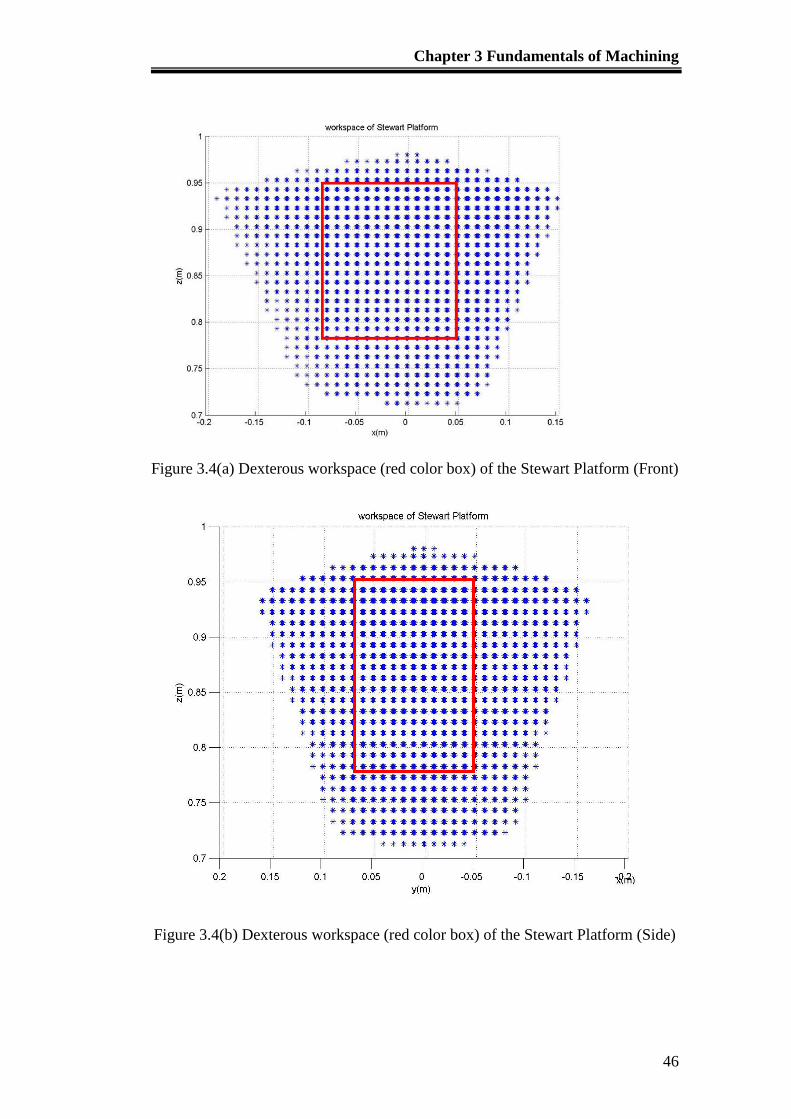
Chapter 3 Fundamentals of Machining
46
Figure 3.4(a) Dexterous workspace (red color box) of the Stewart Platform (Front)
Figure 3.4(b) Dexterous workspace (red color box) of the Stewart Platform (Side)
Chapter 3 Fundamentals of Machining
47
In the literature review of [Reimund, 2000], a stiffness comparison was
done with different design principles, such as Hexaglide which is a parallel
kinematics manipulator with constant strut length while Stewart Platform is a
parallel kinematics manipulator with variable strut length. The comparison
indicates that the Stewart Platform is very homogeneous in the working area as
compared with the Hexaglide. For the parallel kinematics system, no other values
can be specified for an inclination of 30° due to the occurrence of singularities in
this range, whereby the loads approach infinity and the stiffness converges to zero.
As a result, the loads in the structure with constant strut length are greater
than the structure with variable strut length. This is due to the arrangement of the
pivot planes and the center of motion, which imposes limitation on the rotational
motions of the mobile platform.
In term of static stiffness of the tool cutting point, the major cause is the
arrangement of the pivot points. The investigations are based on the position of
the pivot points. The limited workspace of a Stewart Platform introduces
difficulty of achieving accurate motion. Furthermore, gravitation introduces sag
of the platform which is relatively large and inconsistent throughout the
workspace when it is under the weight of the spindle or the workpiece. Even
though the ball-screw actuator is loaded by a pure linear force of tension or
compression, the overall stiffness of the strut is still limited by the stiffness in the
ball-screw/nut contacts, the thrust bearings and the spherical joints at each end of
the strut. As a result, the effective stiffness will be changing throughout the
Chapter 3 Fundamentals of Machining
48
workspace. This will cause a prominent issue of accuracy and induce difficulty in
the compensation of the dynamics of the platform.
During machining processes, stability against chatter is defined by the
stiffness, damping and natural frequency of the most flexible mode of the
vibration of the machining system. The spindle, holder and tool assembly is the
least stiff element in the structure for most machines. For a Stewart Platform, the
ball-screw-driven actuator assembly represents not only the axis drives but also
the entire support structure. In addition, each ball-screw assembly must be
supported at each end by spherical joints at the top and universal joints at the
bottom. The effect of this flexibility causes a very significant reduction in the
overall stiffness. Moreover, each actuator drives the platform at an angle to its
motion, and this causes an unfavorable transmission ratio. The result is that the
stiffness at the platform is rather low as compared to the stiffness of the individual
actuators.
Hence, by applying the ball-screw drive as a classical machining center,
the Stewart Platform is not capable of providing sufficient tool point stiffness to
be useful for high speed milling. The low stiffness together with the variation of
the workspace has led to the problems of deflections under cutting forces, sag due
to the weight of the spindle or workpiece, problems with chatter, overshoot,
general dynamics of the drives and the control system. Nevertheless, a Stewart
Platform can still be designed to be of high stiffness by implementing further
kinematics constraints which it will generate sufficiently for the purpose of high

Chapter 3 Fundamentals of Machining
49
speed machining. With the same basic drive elements implemented, a Stewart
Platform is capable of higher flexibility due to its ability to be manipulated in six
DOF as compared with a classical serial kinematics manipulator.
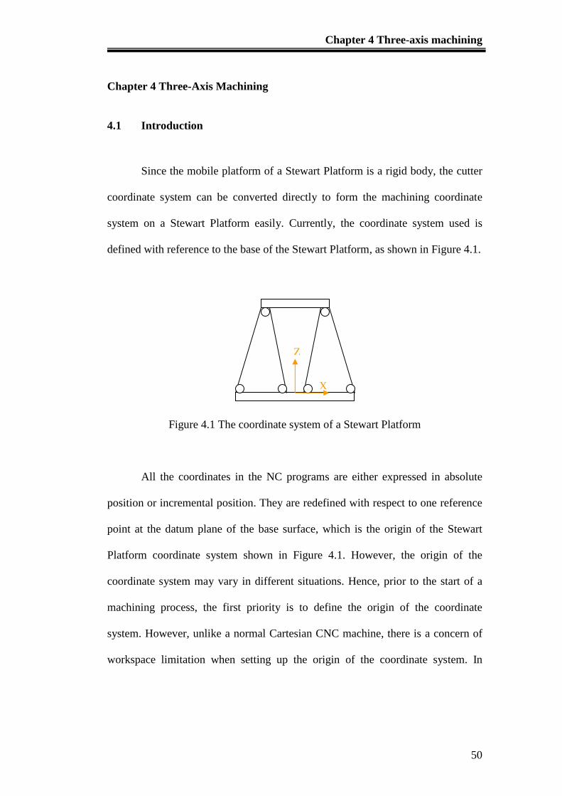
Chapter 4 Three-axis machining
50
Chapter 4 Three-Axis Machining
4.1 Introduction
Since the mobile platform of a Stewart Platform is a rigid body, the cutter
coordinate system can be converted directly to form the machining coordinate
system on a Stewart Platform easily. Currently, the coordinate system used is
defined with reference to the base of the Stewart Platform, as shown in Figure 4.1.
Figure 4.1 The coordinate system of a Stewart Platform
All the coordinates in the NC programs are either expressed in absolute
position or incremental position. They are redefined with respect to one reference
point at the datum plane of the base surface, which is the origin of the Stewart
Platform coordinate system shown in Figure 4.1. However, the origin of the
coordinate system may vary in different situations. Hence, prior to the start of a
machining process, the first priority is to define the origin of the coordinate
system. However, unlike a normal Cartesian CNC machine, there is a concern of
workspace limitation when setting up the origin of the coordinate system. In
Z
X
Z
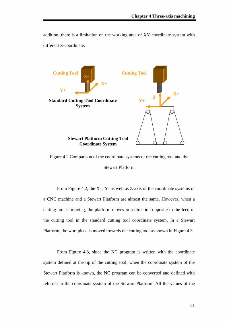
Chapter 4 Three-axis machining
51
addition, there is a limitation on the working area of XY-coordinate system with
different Z-coordinate.
Figure 4.2 Comparison of the coordinate systems of the cutting tool and the
Stewart Platform
From Figure 4.2, the X- , Y- as well as Z-axis of the coordinate systems of
a CNC machine and a Stewart Platform are almost the same. However, when a
cutting tool is moving, the platform moves in a direction opposite to the feed of
the cutting tool in the standard cutting tool coordinate system. In a Stewart
Platform, the workpiece is moved towards the cutting tool as shown in Figure 4.3.
From Figure 4.3, since the NC program is written with the coordinate
system defined at the tip of the cutting tool, when the coordinate system of the
Stewart Platform is known, the NC program can be converted and defined with
referred to the coordinate system of the Stewart Platform. All the values of the
X+
Y+
Z+ Cutting Tool
Standard Cutting Tool Coordinate
System
X+
Y+
Cutting Tool
Z+
Stewart Platform Cutting Tool
Coordinate System
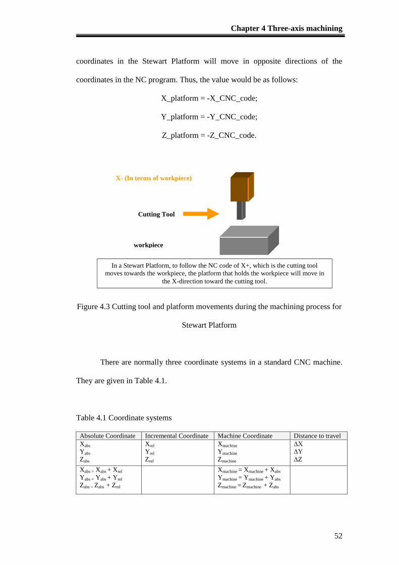
Chapter 4 Three-axis machining
52
coordinates in the Stewart Platform will move in opposite directions of the
coordinates in the NC program. Thus, the value would be as follows:
X_platform = -X_CNC_code;
Y_platform = -Y_CNC_code;
Z_platform = -Z_CNC_code.
Figure 4.3 Cutting tool and platform movements during the machining process for
Stewart Platform
There are normally three coordinate systems in a standard CNC machine.
They are given in Table 4.1.
Table 4.1 Coordinate systems
Absolute Coordinate Incremental Coordinate Machine Coordinate Distance to travel
Xabs
Yabs
Zabs
Xrel
Yrel
Zrel
Xmachine
Ymachine
Zmachine
ΔX
ΔY
ΔZ
Xabs = Xabs + Xrel
Yabs = Yabs + Yrel
Zabs = Zabs + Zrel
Xmachine = Xmachine + Xabs
Ymachine = Ymachine + Yabs
Zmachine = Zmachine + Zabs
X- (In terms of workpiece)
Cutting Tool
workpiece
In a Stewart Platform, to follow the NC code of X+, which is the cutting tool
moves towards the workpiece, the platform that holds the workpiece will move in
the X-direction toward the cutting tool.
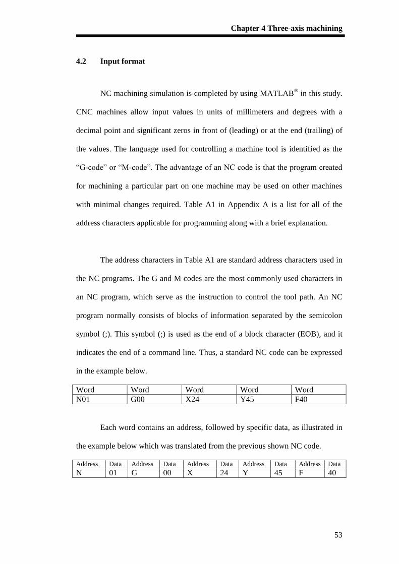
Chapter 4 Three-axis machining
53
4.2 Input format
NC machining simulation is completed by using MATLAB® in this study.
CNC machines allow input values in units of millimeters and degrees with a
decimal point and significant zeros in front of (leading) or at the end (trailing) of
the values. The language used for controlling a machine tool is identified as the
“G-code” or “M-code”. The advantage of an NC code is that the program created
for machining a particular part on one machine may be used on other machines
with minimal changes required. Table A1 in Appendix A is a list for all of the
address characters applicable for programming along with a brief explanation.
The address characters in Table A1 are standard address characters used in
the NC programs. The G and M codes are the most commonly used characters in
an NC program, which serve as the instruction to control the tool path. An NC
program normally consists of blocks of information separated by the semicolon
symbol (;). This symbol (;) is used as the end of a block character (EOB), and it
indicates the end of a command line. Thus, a standard NC code can be expressed
in the example below.
Word Word Word Word Word
N01 G00 X24 Y45 F40
Each word contains an address, followed by specific data, as illustrated in
the example below which was translated from the previous shown NC code.
Address Data Address Data Address Data Address Data Address Data
N 01 G 00 X 24 Y 45 F 40
Chapter 4 Three-axis machining
54
Through an analysis of the address and the respective data, a machining
path can be generated based on the instructions provided by the address.
G codes are the preparatory functions which provide instruction on a
machining path and identifying activities execution activities by the machine. In
NC code, normally there is more than one G-Codes in a program block. Specific
G-codes work as the communication between the machine controller and the
machine tool especially when the machine is performing specific machining
operations. In a G-code, the modal commands remain in effect for multi blocks
until the next new G-code is called to replace the commands from the same group.
In addition there are non-modal G-code commands that are only used once in a
single block.
There are different groups of modal G-codes. One code from each group
may be specified in an individual block. However, if two codes of the same group
appear in the same block, the former one will be ignored and the latter will be
applied in the program. A safety block is a block of G codes which is used as a
code to overwrite any remaining G code from the previous program. Hence, it is a
good habit to implement a safety block after changing a tool or when there is a
need to rerun a single operation within the program. This implementation can help
prevent some unwanted effects left by the previous G-codes.
A few G-codes are active when a machine is started. The items marked
with an * before the G value of Code column, as shown in G-codes chart of Table

Chapter 4 Three-axis machining
55
A2 in Appendix A, are active upon the startup of a machine. G00, G01, G90 and
G91, are the active initial code that is determined by a parameter setting. Normally,
during a start-up condition, the program is set at G01 and G90.
Besides G-codes, M codes also play an important role in an NC program. M
codes serve as the miscellaneous functions that control the working components,
such as the activation of the coolant flow, spindle rotation, direction of the spindle
rotation, etc. Table A3 in Appendix A shows the commonly used M codes in NC
programs.
Based on these guidelines, a post-processor for a Stewart Platform has been
developed to implement an NC program as the trajectory path for 3-axis machining.
All the basic G-codes are translated in the post-processor such that by inputting the
NC program into the post-processor, an appropriate trajectory path can be
generated for the Stewart Platform to perform the required machining process.
Firstly, a model is created using a CAD software, such as SolidWorks, and
exported as a Parasolids file. This file is imported into CAM software, such as
MasterCam, to generate the required NC program to machine out the model. The
generated NC program will be imported into the post-processor that has been
developed in MATLAB® to produce the required trajectory path that will be used
for the actual machining on the Stewart Platform. The format of an NC program is
shown in Figure 4.4.
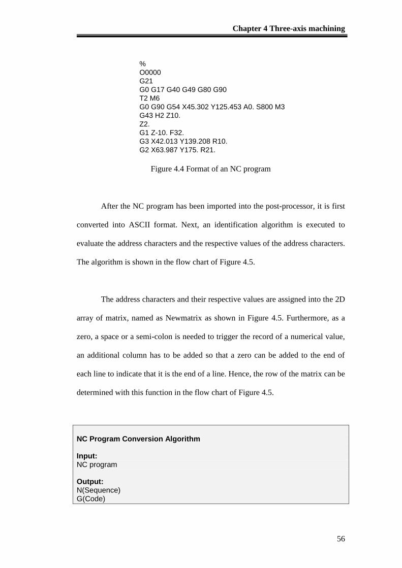
Chapter 4 Three-axis machining
56
%
O0000
G21
G0 G17 G40 G49 G80 G90
T2 M6
G0 G90 G54 X45.302 Y125.453 A0. S800 M3
G43 H2 Z10.
Z2.
G1 Z-10. F32.
G3 X42.013 Y139.208 R10.
G2 X63.987 Y175. R21.
X71.464 Y147.099 R21.
G3 X71.404 Y146.281 R1.
G1 X89.94 Y95.353
G3 X90.792 Y94.699 R1.
G1 X149.37 Y89.574
G3 X150.164 Y89.862 R1.
G2 X179.836 Y60.138 R21.
X150.164 R21.
G3 X149.37 Y60.426 R1.001
G1 X76.83 Y54.08
G2 X54.319 Y71.353 R21.
G1 X42.474 Y138.529
G3 X42.013 Y139.208 R1.
X28.258 Y135.918 R10.
G0 Z10.
M5
G91 G28 Z0.
G28 X0. Y0. A0.
M30
%
Figure 4.4 Format of an NC program
After the NC program has been imported into the post-processor, it is first
converted into ASCII format. Next, an identification algorithm is executed to
evaluate the address characters and the respective values of the address characters.
The algorithm is shown in the flow chart of Figure 4.5.
The address characters and their respective values are assigned into the 2D
array of matrix, named as Newmatrix as shown in Figure 4.5. Furthermore, as a
zero, a space or a semi-colon is needed to trigger the record of a numerical value,
an additional column has to be added so that a zero can be added to the end of
each line to indicate that it is the end of a line. Hence, the row of the matrix can be
determined with this function in the flow chart of Figure 4.5.
NC Program Conversion Algorithm Input: NC program Output: N(Sequence) G(Code)
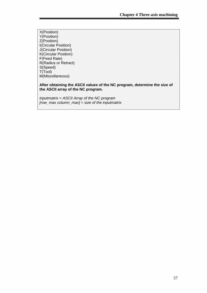
Chapter 4 Three-axis machining
57
X(Position) Y(Position) Z(Position) I(Circular Position) J(Circular Position) K(Circular Position) F(Feed Rate) R(Radius or Retract) S(Speed) T(Tool) M(Miscellaneous) After obtaining the ASCII values of the NC program, determine the size of the ASCII array of the NC program. inputmatrix = ASCII Array of the NC program [row_max column_max] = size of the inputmatrix
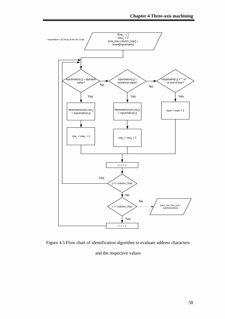
Chapter 4 Three-axis machining
58
Row1 = 1
Row2 = 2
[row_max column_max] =
sizeof[inputmatrix]
Inputmatrix(i,j) = alphabet
value?
Inputmatrix(i,j) =
numerical value?
Inputmatrix(i,j) =”;” or “ “
or end of line?
Newmatrix(num,row1)
= inputmatrix(I,j)
Newmatrix(num,row2)
= inputmatrix(I,j)num = num + 1
row1 = row
1 + 1
row2 = row
2 + 2
j = j + 1
j <= column_max
i <= column_max
i = i + 1
[new_row, new_col] =
size(Newmatrix)
Yes
No
YesYes
No
Yes
Yes
No
No
*inputmatrix = 2D Array of the NC Code
Figure 4.5 Flow chart of identification algorithm to evaluate address characters
and the respective values
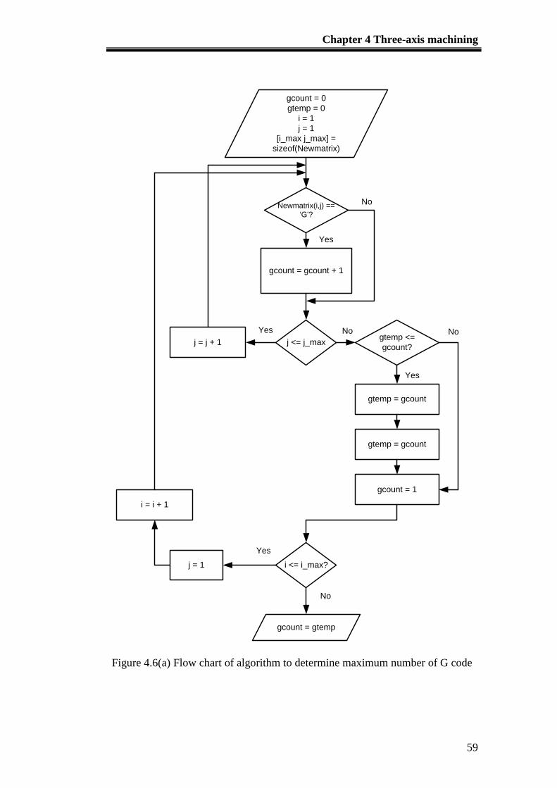
Chapter 4 Three-axis machining
59
gcount = 0
gtemp = 0
i = 1
j = 1
[i_max j_max] =
sizeof(Newmatrix)
Newmatrix(i,j) ==
‘G’?
gcount = gcount + 1
j <= j_max
i <= i_max?
gtemp <=
gcount?
gtemp = gcount
gtemp = gcount
gcount = 1
gcount = gtemp
j = j + 1
i = i + 1
Yes
No
NoYes No
Yes
Yes
No
j = 1
Figure 4.6(a) Flow chart of algorithm to determine maximum number of G code
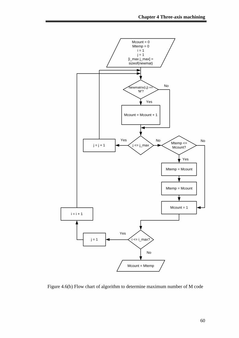
Chapter 4 Three-axis machining
60
Mcount = 0
Mtemp = 0
i = 1
j = 1
[i_max j_max] =
sizeof(newmat)
Newmatrix(i,j) ==
‘M’?
Mcount = Mcount + 1
j <= j_max
i <= i_max?
Mtemp <=
Mcount?
Mtemp = Mcount
Mtemp = Mcount
Mcount = 1
Mcount = Mtemp
j = j + 1
i = i + 1
Yes
No
NoYes No
Yes
Yes
No
j = 1
Figure 4.6(b) Flow chart of algorithm to determine maximum number of M code
Chapter 4 Three-axis machining
61
The matrix, Newmatrix is further categorized into 1D array matrix of the
corresponding address characters code such as X, Y and Z code. However, since
G and M codes can appear more than once in each single line of NC program, an
algorithm is developed to detect the maximum number of G and M code
appearance in each line of the NC program as shown in Figure 4.6(a) and Figure
4.6(b). The flow of the algorithm to assign the matrix size of the respective
character address can be expressed in the flow chart as shown in Figure 4.7.
Therefore, each command block consists of only one specific character
except for characters 'M' and 'G', the arrays of the respective characters can be
determined. The maximum number of G and M characters that appear in an NC
program can also be defined.
As a result, the output of the corresponding character addresses matrix is
obtained for further development of the conversion of the NC program to the
trajectory path recognized by the Stewart Platform. The flow chart of the
algorithm that assigns the NC program character address to the respective matrix
is shown in Figure 4.8.
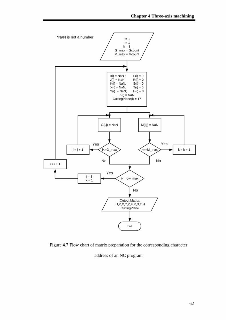
Chapter 4 Three-axis machining
62
i = 1
j = 1
k = 1
G_max = Gcount
M_max = Mcount
I(i) = NaN ; F(i) = 0
J(i) = NaN; R(i) = 0
K(i) = NaN; S(i) = 0
X(i) = NaN; T(i) = 0
Y(i) = NaN; H(i) = 0
Z(i) = NaN
CuttingPlane(i) = 17
*NaN is not a number
G(i,j) = NaN M(i,j) = NaN
j<=G_max k<=M_maxj = j + 1 k = k + 1
i<=row_maxj = 1
k = 1
i = i + 1
End
Output Matrix:
I,J,K,X,Y,Z,F,R,S,T,H
CuttingPlane
Yes
No
Yes
No
No
Yes
Figure 4.7 Flow chart of matrix preparation for the corresponding character
address of an NC program
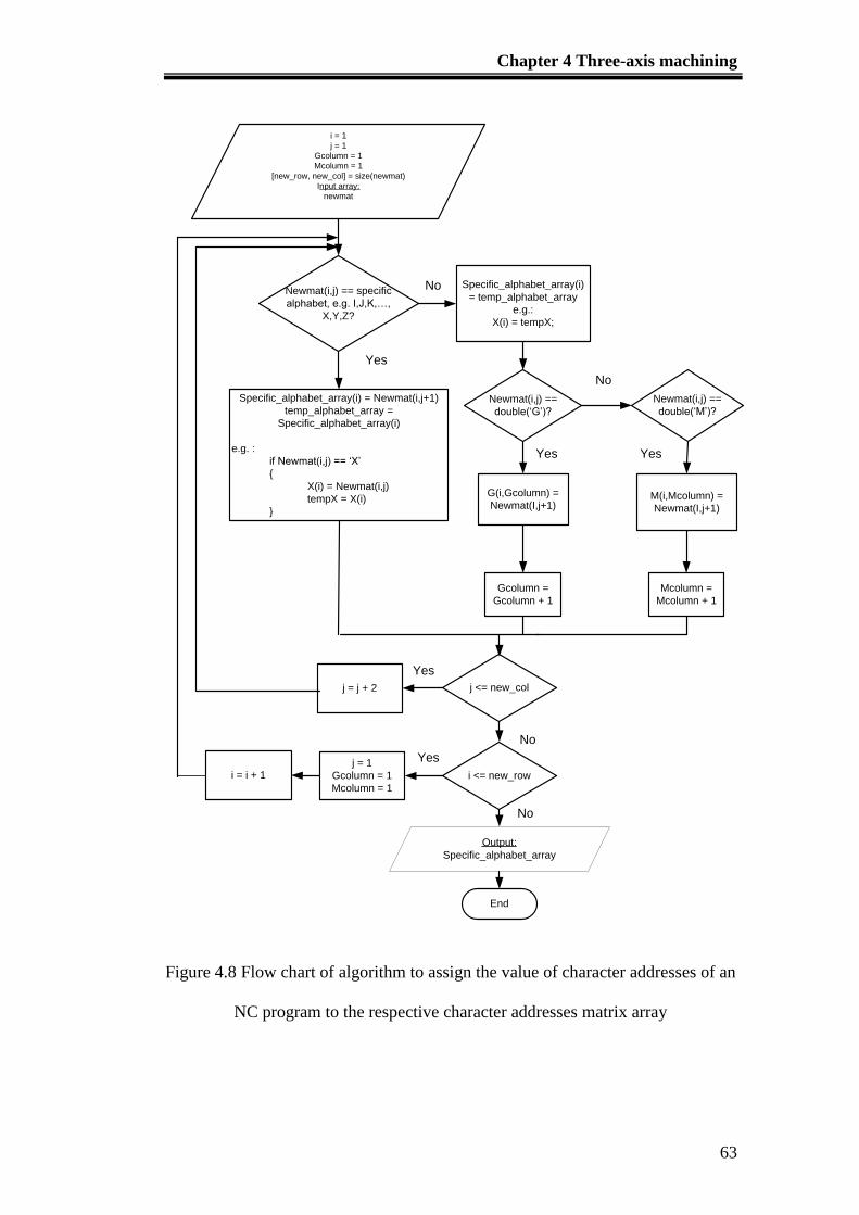
Chapter 4 Three-axis machining
63
i = 1
j = 1
Gcolumn = 1
Mcolumn = 1
[new_row, new_col] = size(newmat)
Input array:
newmat
Newmat(i,j) == specific
alphabet, e.g. I,J,K,…,
X,Y,Z?
Specific_alphabet_array(i) = Newmat(i,j+1)
temp_alphabet_array =
Specific_alphabet_array(i)
e.g. :
if Newmat(i,j) == ‘X’
{
X(i) = Newmat(i,j)
tempX = X(i)
}
Newmat(i,j) ==
double(‘G’)?
Specific_alphabet_array(i)
= temp_alphabet_array
e.g.:
X(i) = tempX;
Newmat(i,j) ==
double(‘M’)?
G(i,Gcolumn) =
Newmat(I,j+1)M(i,Mcolumn) =
Newmat(I,j+1)
Gcolumn =
Gcolumn + 1
Mcolumn =
Mcolumn + 1
j <= new_col
i <= new_row
j = j + 2
j = 1
Gcolumn = 1
Mcolumn = 1
i = i + 1
End
Yes
No
Yes
No
Yes Yes
No
No
Yes
Output:
Specific_alphabet_array
Figure 4.8 Flow chart of algorithm to assign the value of character addresses of an
NC program to the respective character addresses matrix array
Chapter 4 Three-axis machining
64
The purpose of the identification algorithm is to ensure that the post-
processor can recognize important G-codes, namely, G17, G18 and G19. G17 is
the selection of the X-Y plane as the machining plane, which is the default setting.
G18 is the selection of the X-Z plane as the main machining plane for circular
interpolation movements and/or cutter compensation. This G18 code changes the
default machining plane to the X-Z plane where Y-axis is the secondary axis and
it works perpendicularly to the X-Z plane. In the X-Z plane, it is possible to cut
convex or concave surfaces using the G02 and G03 circular interpolation
commands. It should be noted that since the X- and Z-axes are the primary axes
instead of the X- and Y-axes, the radius is no longer expressed in terms of I and J
(distance from the start-point to the center-point; refer to G02 and G03 in Table
5.3) but in terms of I and K. In addition, the determination of the direction of
travel of the tool is based on the view of the user towards the two axes from the
Y+ direction, in the same way as the user looks at the X- and Y-axes from the Z+
axis in the G17 plane. When using the G02 and G03 commands, the primary and
secondary axes are reversed. This means that G02 will look like a
counterclockwise arc and G03 will look like a clockwise arc.
After arranging the values corresponding to the characters, the machining
coordinates can be arranged according to the instructions provided by the 'G' and
'M' codes. Firstly, the post-processor determines the presence of G90 (absolute
coordinates) or G91 (incremental coordinates), by scanning through the array of
the G-codes line-by-line. It helps to determine whether a block command is
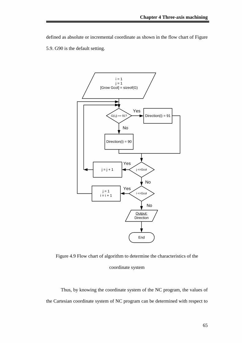
Chapter 4 Three-axis machining
65
defined as absolute or incremental coordinate as shown in the flow chart of Figure
5.9. G90 is the default setting.
i = 1
j = 1
[Grow Gcol] = sizeof(G)
G(i,j) == 91? Direction(i) = 91
Direction(i) = 90
j <=Gcol
i <=Gcol
Output:
Direction
End
j = j + 1
j = 1
i = i + 1
Yes
No
Yes
No
No
Yes
Figure 4.9 Flow chart of algorithm to determine the characteristics of the
coordinate system
Thus, by knowing the coordinate system of the NC program, the values of
the Cartesian coordinate system of NC program can be determined with respect to
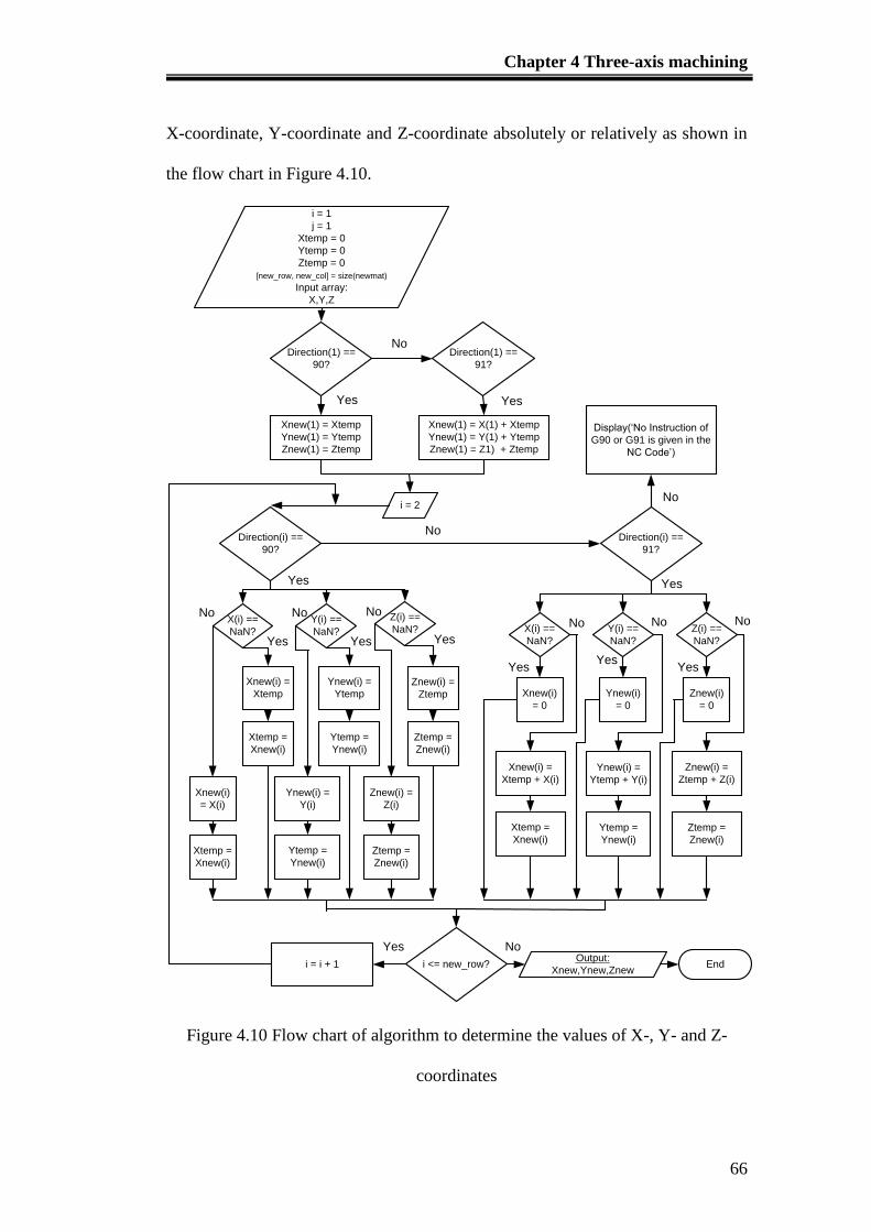
Chapter 4 Three-axis machining
66
X-coordinate, Y-coordinate and Z-coordinate absolutely or relatively as shown in
the flow chart in Figure 4.10.
i = 1
j = 1
Xtemp = 0
Ytemp = 0
Ztemp = 0
[new_row, new_col] = size(newmat)
Input array:
X,Y,Z
Direction(1) ==
90?
Direction(1) ==
91?
Xnew(1) = Xtemp
Ynew(1) = Ytemp
Znew(1) = Ztemp
Xnew(1) = X(1) + Xtemp
Ynew(1) = Y(1) + Ytemp
Znew(1) = Z1) + Ztemp
i = 2
Direction(i) ==
90?
Direction(i) ==
91?
X(i) ==
NaN?
Y(i) ==
NaN?
Z(i) ==
NaN?
Xnew(i)
= X(i)
Xnew(i) =
Xtemp
Ynew(i) =
Ytemp
Ynew(i) =
Y(i)
Znew(i) =
Z(i)
Znew(i) =
Ztemp
X(i) ==
NaN?
Y(i) ==
NaN?
Z(i) ==
NaN?
Xnew(i) =
Xtemp + X(i)
Xnew(i)
= 0
Ynew(i)
= 0
Ynew(i) =
Ytemp + Y(i)
Znew(i) =
Ztemp + Z(i)
Znew(i)
= 0
Xtemp =
Xnew(i)
Ytemp =
Ynew(i)
Ztemp =
Znew(i)Xtemp =
Xnew(i)
Ytemp =
Ynew(i)
Ztemp =
Znew(i)
Xtemp =
Xnew(i)
Ytemp =
Ynew(i)
Ztemp =
Znew(i)
i <= new_row?Output:
Xnew,Ynew,ZnewEndi = i + 1
Yes
No
No
Yes Yes
Display(‘No Instruction of
G90 or G91 is given in the
NC Code’)
No
Yes
Yes Yes Yes
YesYes
Yes
NoNoNoNo No No
NoYes
Figure 4.10 Flow chart of algorithm to determine the values of X-, Y- and Z-
coordinates
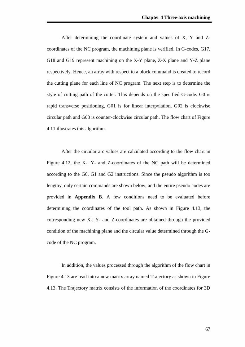
Chapter 4 Three-axis machining
67
After determining the coordinate system and values of X, Y and Z-
coordinates of the NC program, the machining plane is verified. In G-codes, G17,
G18 and G19 represent machining on the X-Y plane, Z-X plane and Y-Z plane
respectively. Hence, an array with respect to a block command is created to record
the cutting plane for each line of NC program. The next step is to determine the
style of cutting path of the cutter. This depends on the specified G-code. G0 is
rapid transverse positioning, G01 is for linear interpolation, G02 is clockwise
circular path and G03 is counter-clockwise circular path. The flow chart of Figure
4.11 illustrates this algorithm.
After the circular arc values are calculated according to the flow chart in
Figure 4.12, the X-, Y- and Z-coordinates of the NC path will be determined
according to the G0, G1 and G2 instructions. Since the pseudo algorithm is too
lengthy, only certain commands are shown below, and the entire pseudo codes are
provided in Appendix B. A few conditions need to be evaluated before
determining the coordinates of the tool path. As shown in Figure 4.13, the
corresponding new X-, Y- and Z-coordinates are obtained through the provided
condition of the machining plane and the circular value determined through the G-
code of the NC program.
In addition, the values processed through the algorithm of the flow chart in
Figure 4.13 are read into a new matrix array named Trajectory as shown in Figure
4.13. The Trajectory matrix consists of the information of the coordinates for 3D
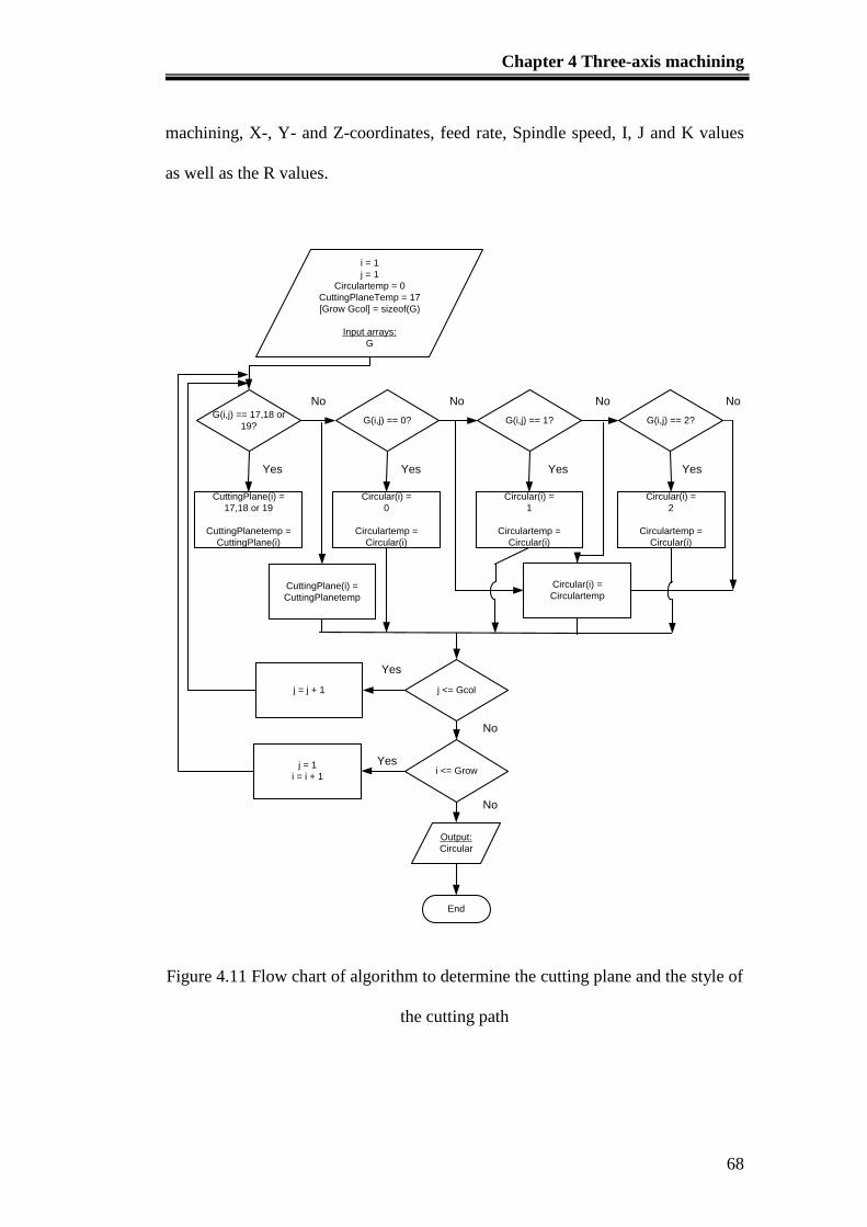
Chapter 4 Three-axis machining
68
machining, X-, Y- and Z-coordinates, feed rate, Spindle speed, I, J and K values
as well as the R values.
i = 1
j = 1
Circulartemp = 0
CuttingPlaneTemp = 17
[Grow Gcol] = sizeof(G)
Input arrays:
G
G(i,j) == 17,18 or
19?G(i,j) == 0? G(i,j) == 1? G(i,j) == 2?
CuttingPlane(i) =
17,18 or 19
CuttingPlanetemp =
CuttingPlane(i)
CuttingPlane(i) =
CuttingPlanetemp
Circular(i) =
0
Circulartemp =
Circular(i)
Circular(i) =
1
Circulartemp =
Circular(i)
Circular(i) =
2
Circulartemp =
Circular(i)
Circular(i) =
Circulartemp
j <= Gcol
i <= Grow
Output:
Circular
End
j = 1
i = i + 1
j = j + 1
Yes
No
No No No No
Yes Yes Yes Yes
Yes
No
Figure 4.11 Flow chart of algorithm to determine the cutting plane and the style of
the cutting path
Chapter 4 Three-axis machining
69
Figure 4.12(a) Flow chart of algorithm to convert NC program to machine
trajectory
i = 1
num = 1[new_row, new_col] =
sizeof(newmat)
Input arrays:
CuttingPlane
Xnew,Ynew,Znew,I,J,K,R
CuttingPlane(i)
== 17?
CuttingPlane(i)
== 18?
CuttingPlane(i)
== 19?
x2 = Xnew(i)
y2 = Ynew(i)z2 = Znew(i)
x2 = Xnew(i)y2 = Znew(i)
z2 = Ynew(i)
x2 = Ynew(i)y2 = Znew(i)
z2 = Xnew(i)
i-1>0 i-1>0 i-1>0
x1 = Xnew(i-1)
y1 = Ynew(i-1)
z1 = Znew(i-1)
x1 = 0y1 = 0
z1 = 0
x1 = 0y1 = 0
z1 = 0
x1 = 0y1 = 0
z1 = 0
x1 = Xnew(i-1)
y1 = Znew(i-1)
z1 = Ynew(i-1)
x1 = Ynew(i-1)
y1 = Znew(i-1)
z1 = Xnew(i-1)
R = Radius of the circular path Condition 1 : G0 and G1 is given while R = 0
coordinate = [Xnew(i) Ynew(i) Znew(i)]; Condition 2 : Clockwise(CW) circular path with R only coordinate = arcR(1,x1,y1,x2,y2,R(i));
Condition 3 : CW circular path with IJ coordinate = clockwise(x1,y1,x2,y2,I(i),J(i));
Condition 4 : CW circular path with IK coordinate = clockwise(x1,y1,x2,y2,I(i),K(i)); Condition 5 : CW circular path with JK
coordinate = clockwise(x1,y1,x2,y2,J(i),K(i)); Condition 6 : CounterClockwise(CCW) circular path with R only coordinate = arcR(2,x1,y1,x2,y2,R(i)); Condition 7 : CCW circular path with IJ coordinate = anticlockwise(x1,y1,x2,y2,I(i),J(i)); Condition 8 : CCW circular path with IK coordinate = clockwise(x1,y1,x2,y2,I(i),K(i));
Condition 9 : CCW circular path with JK coordinate = anticlockwise(x1,y1,x2,y2,J(i),K(i));
[Coordrow CoordCol] =
sizeof(coordinate)
1b1a
NoNo
Yes Yes Yes
No No No
Yes Yes Yes
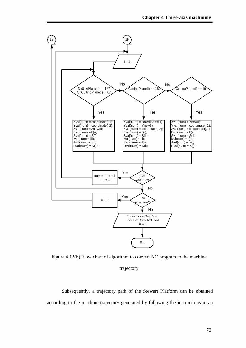
Chapter 4 Three-axis machining
70
Figure 4.12(b) Flow chart of algorithm to convert NC program to the machine
trajectory
Subsequently, a trajectory path of the Stewart Platform can be obtained
according to the machine trajectory generated by following the instructions in an
1b1a
j = 1
CuttingPlane(i) == 17?Or CuttingPlane(i)== 0?
CuttingPlane(i) == 18? CuttingPlane(i) == 19?
Xval(num) = coordinate(j,1);Yval(num) = coordinate(j,2);Zval(num) = Znew(i);Fval(num) = F(i);Sval(num) = S(i);Ival(num) = I(i);Jval(num) = J(i);Rval(num) = K(i);
Xval(num) = coordinate(j,1);Yval(num) = Ynew(i);Zval(num) = coordinate(j,2);Fval(num) = F(i);Sval(num) = S(i);Ival(num) = I(i);Jval(num) = J(i);Rval(num) = K(i);
Xval(num) = Xnew(i);Yval(num) = coordinate(j,1);Zval(num) = coordinate(j,2);Fval(num) = F(i);Sval(num) = S(i);Ival(num) = I(i);Jval(num) = J(i);Rval(num) = K(i);
j <=Coordrow?
i <=new_row?
Trajectory = [Xval YvalZval Fval Sval Ival Jval
Rval]
End
num = num + 1j = j + 1
i = i + 1
No No
Yes Yes Yes
Yes
Yes
No
No
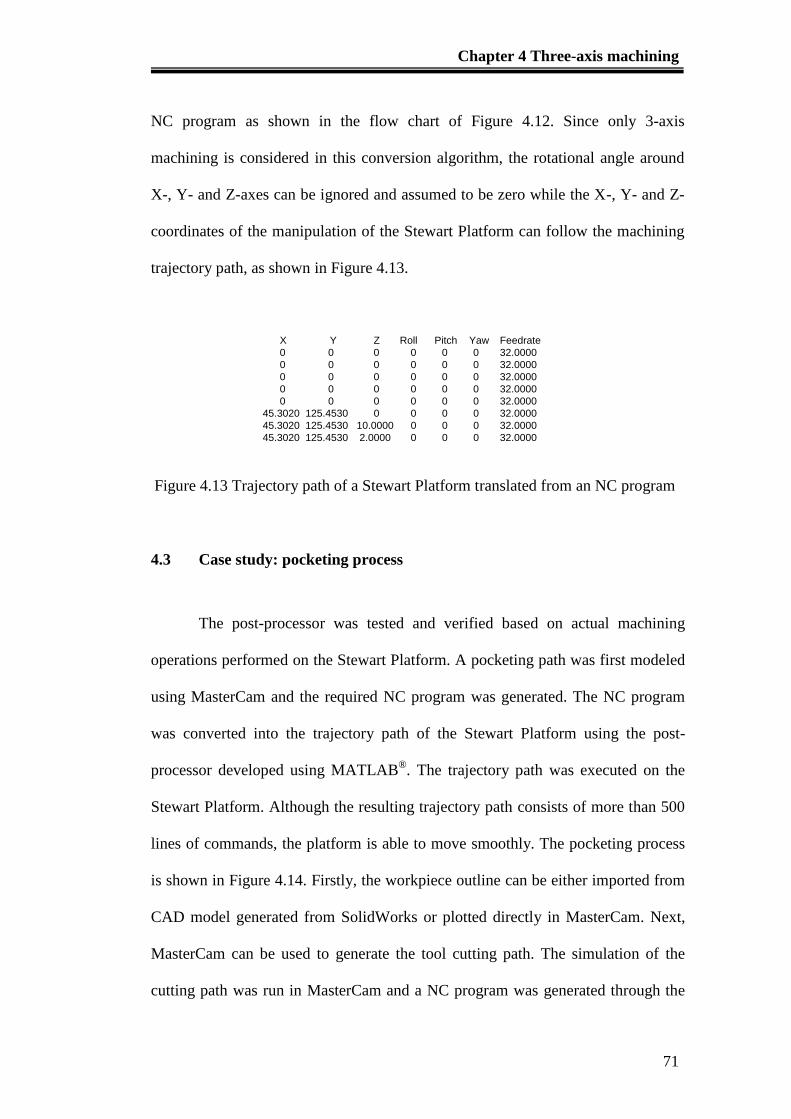
Chapter 4 Three-axis machining
71
NC program as shown in the flow chart of Figure 4.12. Since only 3-axis
machining is considered in this conversion algorithm, the rotational angle around
X-, Y- and Z-axes can be ignored and assumed to be zero while the X-, Y- and Z-
coordinates of the manipulation of the Stewart Platform can follow the machining
trajectory path, as shown in Figure 4.13.
X Y Z Roll Pitch Yaw Feedrate
0 0 0 0 0 0 32.0000
0 0 0 0 0 0 32.0000
0 0 0 0 0 0 32.0000
0 0 0 0 0 0 32.0000
0 0 0 0 0 0 32.0000
45.3020 125.4530 0 0 0 0 32.0000
45.3020 125.4530 10.0000 0 0 0 32.0000
45.3020 125.4530 2.0000 0 0 0 32.0000
Figure 4.13 Trajectory path of a Stewart Platform translated from an NC program
4.3 Case study: pocketing process
The post-processor was tested and verified based on actual machining
operations performed on the Stewart Platform. A pocketing path was first modeled
using MasterCam and the required NC program was generated. The NC program
was converted into the trajectory path of the Stewart Platform using the post-
processor developed using MATLAB®. The trajectory path was executed on the
Stewart Platform. Although the resulting trajectory path consists of more than 500
lines of commands, the platform is able to move smoothly. The pocketing process
is shown in Figure 4.14. Firstly, the workpiece outline can be either imported from
CAD model generated from SolidWorks or plotted directly in MasterCam. Next,
MasterCam can be used to generate the tool cutting path. The simulation of the
cutting path was run in MasterCam and a NC program was generated through the
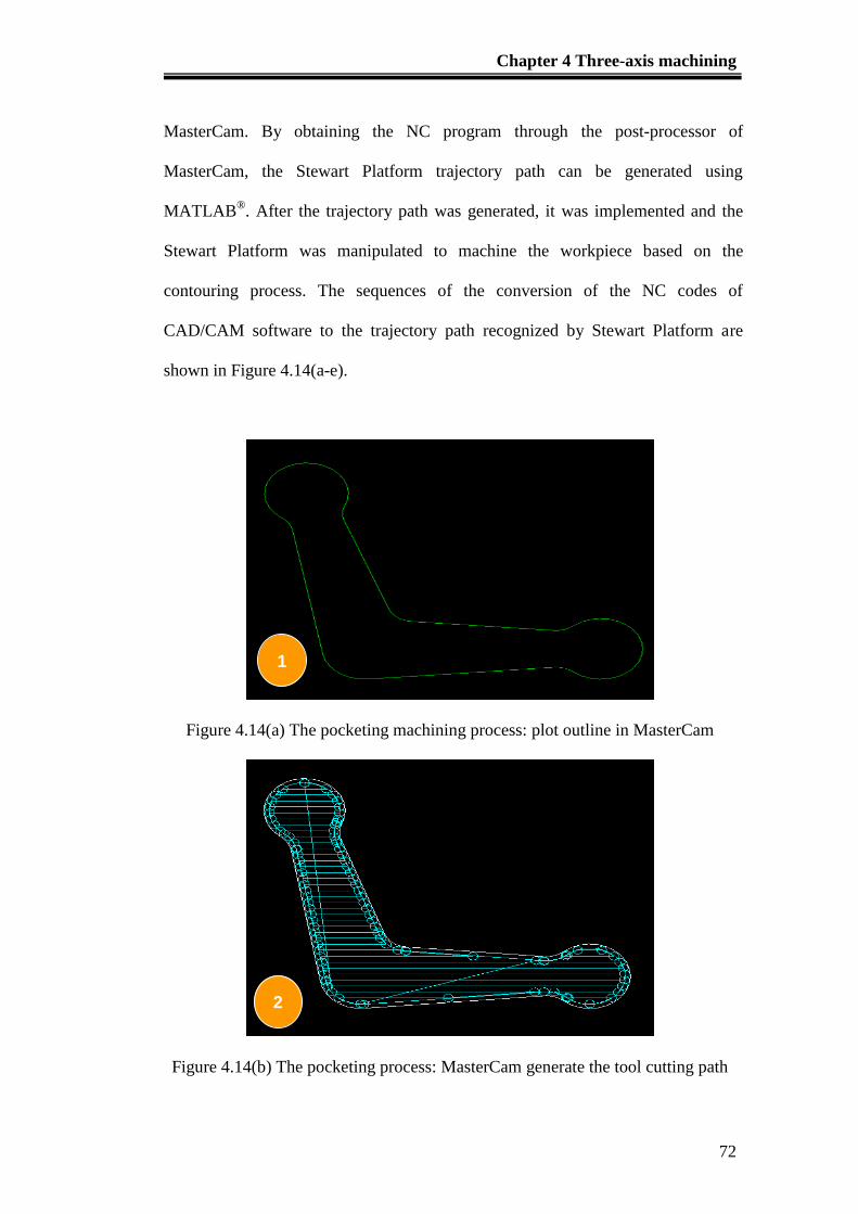
Chapter 4 Three-axis machining
72
MasterCam. By obtaining the NC program through the post-processor of
MasterCam, the Stewart Platform trajectory path can be generated using
MATLAB®. After the trajectory path was generated, it was implemented and the
Stewart Platform was manipulated to machine the workpiece based on the
contouring process. The sequences of the conversion of the NC codes of
CAD/CAM software to the trajectory path recognized by Stewart Platform are
shown in Figure 4.14(a-e).
Figure 4.14(a) The pocketing machining process: plot outline in MasterCam
Figure 4.14(b) The pocketing process: MasterCam generate the tool cutting path
1
2
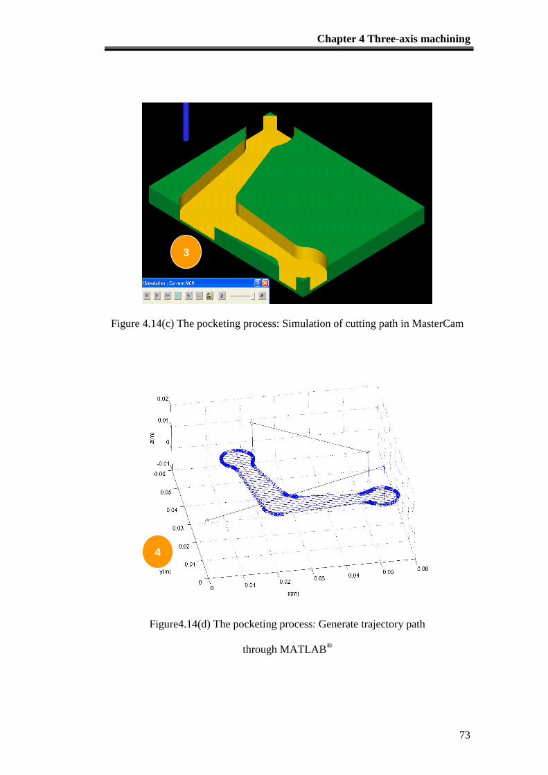
Chapter 4 Three-axis machining
73
Figure 4.14(c) The pocketing process: Simulation of cutting path in MasterCam
Figure4.14(d) The pocketing process: Generate trajectory path
through MATLAB®
3
4

Chapter 4 Three-axis machining
74
Figure 4.14(e) The pocketing process: Machine workpiece through the contouring
process
4.4 Case study: three-axis machining
NC program conversion for 3D machining paths was also developed using
MATLAB®. As shown in Figure 4.15, a 3D hemi-sphere milling path was
generated for a 3D NC program generated from the MasterCam.
A trajectory path for the rough cut was first generated to machine the
outline of the surface of the workpiece using a flat end milling cutter. Next, a
trajectory path for the finishing cut was generated for machining the surface of the
workpiece using a ball-end milling cutter. Figure 4.16 shows the outcome of the
machining performed on a Stewart Platform.
5
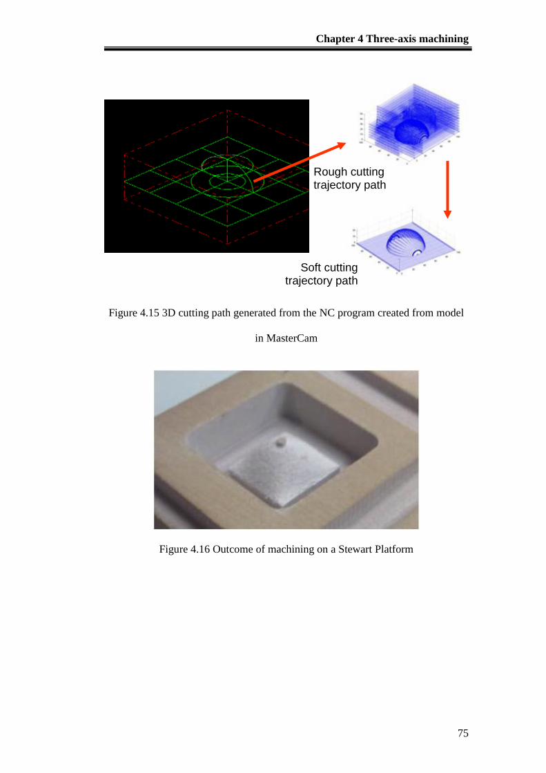
Chapter 4 Three-axis machining
75
Figure 4.15 3D cutting path generated from the NC program created from model
in MasterCam
Figure 4.16 Outcome of machining on a Stewart Platform
Rough cutting trajectory path
Soft cutting trajectory path
Chapter 5 Five-axis machining
76
Chapter 5 Five-axis machining
5.1 Introduction
As described in Chapter 4, 3-axis machining can be performed easily on a
Stewart Platform due to the common characteristics shared by parallel kinematics
manipulators and CNC machines. Hence, minimum effort is required to convert
an NC program from a SolidWorks file to the trajectory path of the Stewart
Platform. Stewart Platforms can be manipulated to perform translation motion for
3-axis machining in the same manner as a serial manipulator since the end-
effectors of both systems are rigid bodies.
However, many considerations need to be looked into due to the
fundamental mechanical design differences between 5-axis CNC machines and
Stewart Platforms, especially when there are rotational movements. This is due to
the fact that the joint errors of the serial manipulators are accumulated and
amplified from joints between links because all joints are dependent on each other
and they are open loop chains. Hence, rotational motions of the joints will give
rise to complicated coordinates of the end-effector. Similarly, Stewart Platforms
can provide very straight-forward joint manipulation because the rotation and
translation of the end-effector can be converted to the joint movement of the
actuator easily using the inverse kinematics algorithm. As a result, Stewart
Platforms have greater advantages over serial manipulators and they can be
controlled easily for 5-axis machining. However, there are some disadvantages of
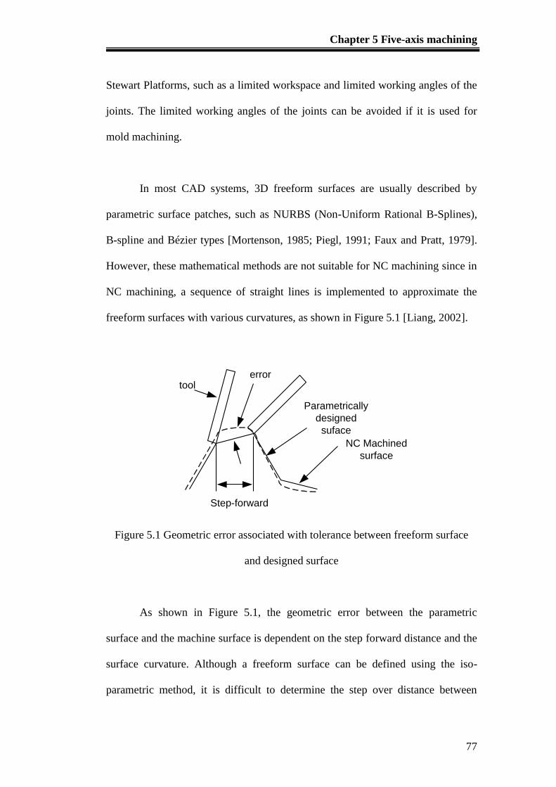
Chapter 5 Five-axis machining
77
Stewart Platforms, such as a limited workspace and limited working angles of the
joints. The limited working angles of the joints can be avoided if it is used for
mold machining.
In most CAD systems, 3D freeform surfaces are usually described by
parametric surface patches, such as NURBS (Non-Uniform Rational B-Splines),
B-spline and Bézier types [Mortenson, 1985; Piegl, 1991; Faux and Pratt, 1979].
However, these mathematical methods are not suitable for NC machining since in
NC machining, a sequence of straight lines is implemented to approximate the
freeform surfaces with various curvatures, as shown in Figure 5.1 [Liang, 2002].
errortool
Parametrically
designed
suface
NC Machined
surface
Step-forward
Figure 5.1 Geometric error associated with tolerance between freeform surface
and designed surface
As shown in Figure 5.1, the geometric error between the parametric
surface and the machine surface is dependent on the step forward distance and the
surface curvature. Although a freeform surface can be defined using the iso-
parametric method, it is difficult to determine the step over distance between
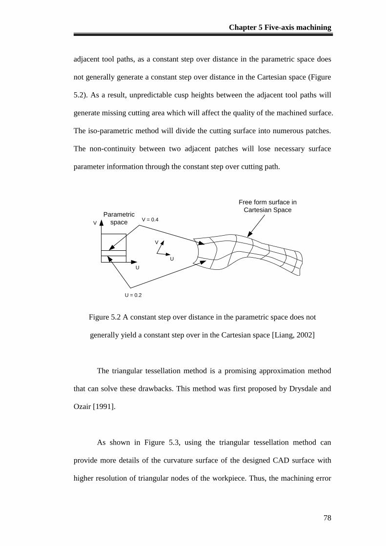
Chapter 5 Five-axis machining
78
adjacent tool paths, as a constant step over distance in the parametric space does
not generally generate a constant step over distance in the Cartesian space (Figure
5.2). As a result, unpredictable cusp heights between the adjacent tool paths will
generate missing cutting area which will affect the quality of the machined surface.
The iso-parametric method will divide the cutting surface into numerous patches.
The non-continuity between two adjacent patches will lose necessary surface
parameter information through the constant step over cutting path.
Parametric
space
V
U
V
U
V = 0.4
U = 0.2
Free form surface in
Cartesian Space
Figure 5.2 A constant step over distance in the parametric space does not
generally yield a constant step over in the Cartesian space [Liang, 2002]
The triangular tessellation method is a promising approximation method
that can solve these drawbacks. This method was first proposed by Drysdale and
Ozair [1991].
As shown in Figure 5.3, using the triangular tessellation method can
provide more details of the curvature surface of the designed CAD surface with
higher resolution of triangular nodes of the workpiece. Thus, the machining error
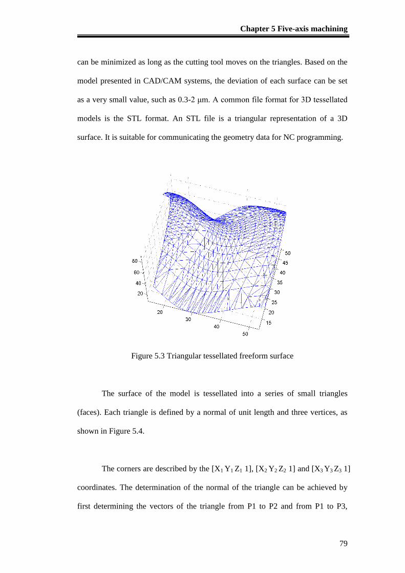
Chapter 5 Five-axis machining
79
can be minimized as long as the cutting tool moves on the triangles. Based on the
model presented in CAD/CAM systems, the deviation of each surface can be set
as a very small value, such as 0.3-2 μm. A common file format for 3D tessellated
models is the STL format. An STL file is a triangular representation of a 3D
surface. It is suitable for communicating the geometry data for NC programming.
Figure 5.3 Triangular tessellated freeform surface
The surface of the model is tessellated into a series of small triangles
(faces). Each triangle is defined by a normal of unit length and three vertices, as
shown in Figure 5.4.
The corners are described by the [X1 Y1 Z1 1], [X2 Y2 Z2 1] and [X3 Y3 Z3 1]
coordinates. The determination of the normal of the triangle can be achieved by
first determining the vectors of the triangle from P1 to P2 and from P1 to P3,

Chapter 5 Five-axis machining
80
which are [Vx1 Vy1 Vz1 0] = [X2-X1 Y2-Y1 Z2-Z1 0] and [Vx2 Vy2 Vz2 0] = [X3-X1
Y3-Y1 Z3-Z1 0]. Thus, the normal of the triangle is Vn = [Xn Yn Zn 0] = [Vx1 Vy1 Vz1
0] x [Vx2 Vy2 Vz2 0]. The length of the normal of the triangle is
222
nnnn ZYXL . Hence, the unit vector of the normal is Vn/Ln. The
orientation of the triangle is based on the right hand rule which direction of the
unit vector of the triangle is always pointing outwards while the vertices are
defined in the counterclockwise direction.
Figure 5.4 Standard triangular representation of STL model
However, there are disadvantages associated with tessellated surfaces,
such as accuracy and resolution. Accuracy is an issue since a tessellated surface is
an approximation of the original surface such that the curve surfaces are uneven as
they are formed by a collection of lines and points. In NC machining, the
contouring movements are composed of linear movements. Hence, the triangular
Vertice 1
Vertice 2 Vertice 3CCW
Out
1
1
1
1
Z
Y
X
1
3
3
3
Z
Y
X
1
2
2
2
Z
Y
X
0
n
n
n
Z
Y
X
V1
V2
V3
Chapter 5 Five-axis machining
81
dimension resolution of the tessellated surfaces can be improved to 0.001mm to
reduce the unevenness.
The number of triangles and the resolution applied to the original surfaces
will determine the size of an STL file. Normally, the size of the file is inversely
proportional to the resolution level and proportional to the number of triangles.
STL files can be generated in two formats, namely, the ASCII and binary formats.
In this research project, the ASCII format is chosen because this format can be
easily read with any text editor and errors can be spotted easily. In addition, the
ASCII format of the STL file can be easily interpreted by the MATLAB®
and
converted into an array of vertices of the tessellated triangles and translated into
the suitable trajectory path.
Another issue needs to be considered is the edit-ability of the STL files.
This is due to the fact that when the STL files are exported from the CAD/CAM
system, it is very hard to perform any further modification. Thus, the CAM
system must rely on the CAD system to produce a good quality STL
representation and suitable tolerance. The tolerance of the tessellated surfaces
must be chosen in anticipation of the tightest machining tolerance under a
particular specification.
5.2 Planar tool paths
Since the step over distance using iso-parametric method is hard to apply
in the generation of tool paths, parallel cutting planes can be used to generate tool
Chapter 5 Five-axis machining
82
paths instead. The advantages of implementing planar movement are that it can
overcome the topological inconsistencies such as overlapping of surface patches,
small gaps between surface patches.
Data from the STL model are used by an algorithm to slice the tessellated
surface by perpendicular cutting planes with predefined interval. The intercepted
coordinates between the tessellated surface and the cutting plane will determine
the 2D cross-sections of the 3D STL models. It could readily be turned into a
physical prototype for Rapid Prototyping (RP) machines. Since these slicing
planes are quite similar to that of a NC milling tool path, the cutting plane
principles used in RP can be applied to the construction of planar tool paths on the
STL freeform surfaces.
In this research, a flat-end milling cutter is used instead of a ball-end
milling cutter for 5-axis machining since the focus is on the milling of surfaces
with limited curvature profiles due to the limited working angle of the Stewart
Platform. The flat-end milling cutter has a more effective radius and a larger
cutting area so that more materials can be removed than using a ball-end milling
cutter. Hence, it can provide a higher productivity. A flat-end milling cutter is also
more suitable for producing large and complex parts, such as turbines. However, a
flat-end cutter has the potential problem of accidentally cutting an adjacent feature
due to tool collision. Thus, in this study the experiment is focused on dealing with
less intricate features.
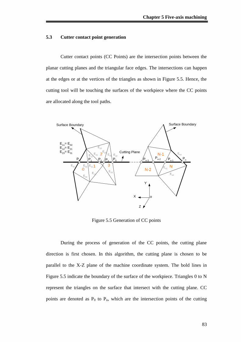
Chapter 5 Five-axis machining
83
5.3 Cutter contact point generation
Cutter contact points (CC Points) are the intersection points between the
planar cutting planes and the triangular face edges. The intersections can happen
at the edges or at the vertices of the triangles as shown in Figure 5.5. Hence, the
cutting tool will be touching the surfaces of the workpiece where the CC points
are allocated along the tool paths.
P0 P
1P
2 P3
P5
01
2
3E01 E
02
E03
E11
E12
E13
E21
E22
E23
E31 E
32
E33
E11
= E02
E12
= E21
E23
= E31 Cutting Plane
N
N-1
N-2
PnP
n-1P
n-2Pn-3
En3
En1
En2
Y
X
Z
o
Surface BoundarySurface Boundary
Figure 5.5 Generation of CC points
During the process of generation of the CC points, the cutting plane
direction is first chosen. In this algorithm, the cutting plane is chosen to be
parallel to the X-Z plane of the machine coordinate system. The bold lines in
Figure 5.5 indicate the boundary of the surface of the workpiece. Triangles 0 to N
represent the triangles on the surface that intersect with the cutting plane. CC
points are denoted as P0 to Pn, which are the intersection points of the cutting

Chapter 5 Five-axis machining
84
plane with the edges of the triangles along the cutting plane. When P0 lies on the
edge E01 of Triangle 0 as shown in Figure 5.5, the next CC point P1 should lie on
the one of the remaining two edges E02 or E03 of Triangle 0. If P1 is found on E03,
the next step would be to determine whether there is another face sharing the same
edge as Triangle 0. Assuming that Triangle 1 shares edge E03 with Triangle 0, and
that edge is E11, the search continues with the remaining two edges of Triangle 1,
E12 and E13 to check for intersection with the cutting plane. Suppose that E12
contains the third CC point P2, the search goes on to find the triangle that shares
E12 with Triangle 1. For the last CC point, Pn which is located at the boundary of
the surface, there would be no adjacent triangle that shares En3. Hence, the search
will end at Pn. The tool path is finally obtained by connecting all the CC points,
from P0 to Pn.
The identification of the intersecting coordinates of the faces and the
planes can be illustrated in the simple algorithm as shown in Figure 5.6. Normally
in the tessellated triangles of the freeform surface as shown in Figure 5.6, certain
faces will intersect with the specific cutting plane. The intersected face has
maximum three edges contact with the cutting plane in three intersected points.
The intersected point can be verified by the factor α. Factor α can be defined by
knowing the cutting plane and vertices of the intersected triangle. By using simple
vector geometry calculation, as long as α >= -1 and α <= 0, the intersected points
will stay within the length of the edge of the triangle. Similarly, the intersected
points will be located at the coordinate which is not within the edge length of the
triangle as shown by IP1 in the diagram.
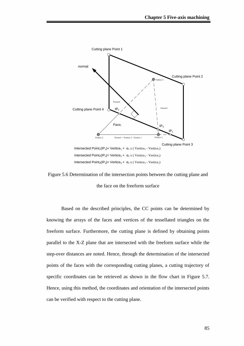
Chapter 5 Five-axis machining
85
Cutting plane Point 2
Cutting plane Point 1
Cutting plane Point 4
Cutting plane Point 3
normal
Vector1 = Vertice 2 - Vertice 1
Vector2
Vector3
Vertice 1Vertice 2
Vertice 3
Intersected Point1(IP1)= Vertice1 + α1 x ( Vertice2 - Vertice1)
Intersected Point2(IP2)= Vertice2 + α2 x ( Vertice3 - Vertice2)
Intersected Point3(IP3)= Vertice3 + α3 x ( Vertice3 - Vertice1)
IP1
IP2
IP3Facei
Figure 5.6 Determination of the intersection points between the cutting plane and
the face on the freeform surface
Based on the described principles, the CC points can be determined by
knowing the arrays of the faces and vertices of the tessellated triangles on the
freeform surface. Furthermore, the cutting plane is defined by obtaining points
parallel to the X-Z plane that are intersected with the freeform surface while the
step-over distances are noted. Hence, through the determination of the intersected
points of the faces with the corresponding cutting planes, a cutting trajectory of
specific coordinates can be retrieved as shown in the flow chart in Figure 5.7.
Hence, using this method, the coordinates and orientation of the intersected points
can be verified with respect to the cutting plane.
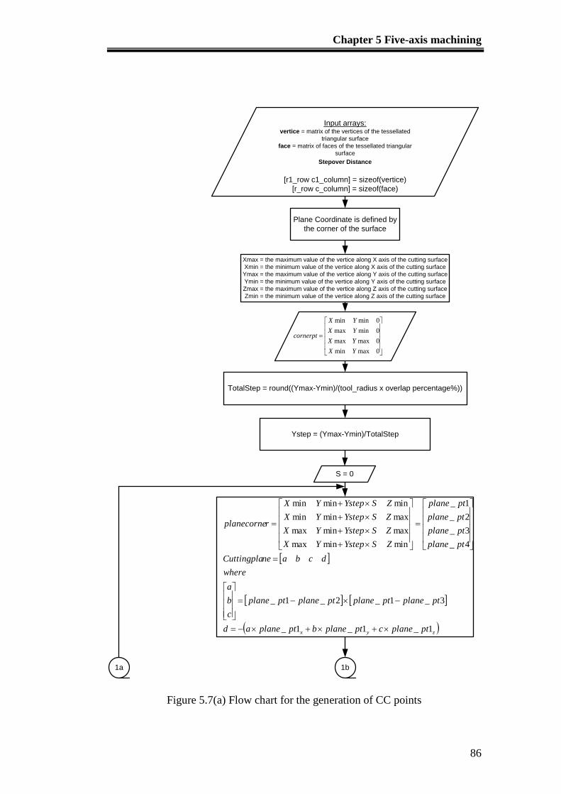
Chapter 5 Five-axis machining
86
Input arrays:vertice = matrix of the vertices of the tessellated
triangular surface
face = matrix of faces of the tessellated triangular
surface
Stepover Distance
[r1_row c1_column] = sizeof(vertice)
[r_row c_column] = sizeof(face)
Plane Coordinate is defined by
the corner of the surface
Xmax = the maximum value of the vertice along X axis of the cutting surface
Xmin = the minimum value of the vertice along X axis of the cutting surface
Ymax = the maximum value of the vertice along Y axis of the cutting surface
Ymin = the minimum value of the vertice along Y axis of the cutting surface
Zmax = the maximum value of the vertice along Z axis of the cutting surface
Zmin = the minimum value of the vertice along Z axis of the cutting surface
TotalStep = round((Ymax-Ymin)/(tool_radius x overlap percentage%))
Ystep = (Ymax-Ymin)/TotalStep
S = 0
1b1a
zyx ptplanecptplanebptplanead
ptplaneptplaneptplaneptplane
c
b
a
where
dcbaneCuttingpla
ptplane
ptplane
ptplane
ptplane
ZSYstepYX
ZSYstepYX
ZSYstepYX
ZSYstepYX
rplanecorne
1_1_1_
3_1_2_1_
4_
3_
2_
1_
minminmax
maxminmax
maxminmin
minminmin
0maxmin
0maxmax
0minmax
0minmin
YX
YX
YX
YX
cornerpt
Figure 5.7(a) Flow chart for the generation of CC points
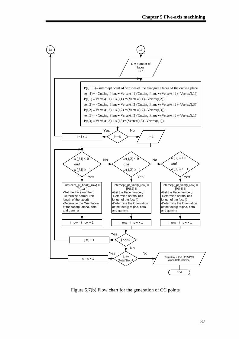
Chapter 5 Five-axis machining
87
1b1a
N = number of
faces
i = 1
));Vertex(i,1-3)(Vertex(i,* i,3)( )Vertex(i,3 P(i,3)
))Vertex(i,1-3)(Vertex(i,Plane )/CuttingVertex(i,3Plane Cutting - i,3)(
));Vertex(i,3-2)(Vertex(i,* i,2)( )Vertex(i,2 P(i,2)
))Vertex(i,3-2)(Vertex(i,Plane )/CuttingVertex(i,2Plane Cutting - i,2)(
));Vertex(i,2-1)(Vertex(i,* i,1)( )Vertex(i,1 P(i,1)
))Vertex(i,1-2)(Vertex(i,Plane )/CuttingVertex(i,1Plane Cutting - (i,1)
plane cutting theof facesr triangula theof verticesofpoint intercept P(i,1..3)
i <=N j = 1
1)1,(
0)1,(
j
and
j
1)2,(
0)2,(
j
and
j
1)3,(
0)3,(
j
and
j
Intercept_pt_final(i_row) =
[P(i,1) j]
-Get the Face number,j
-Determine normal unit
length of the face(j)
-Determine the Orientation
of the face(j) :alpha, beta
and gamma
Intercept_pt_final(i_row) =
[P(i,2) j]
-Get the Face number,j
-Determine normal unit
length of the face(j)
-Determine the Orientation
of the face(j) :alpha, beta
and gamma
Intercept_pt_final(i_row) =
[P(i,3) j]
-Get the Face number,j
-Determine normal unit
length of the face(j)
-Determine the Orientation
of the face(j) :alpha, beta
and gamma
i_row = i_row + 1 i_row = i_row + 1 i_row = i_row + 1
j <=N?j = j + 1
S <=
TotalStep?s = s + 1
Trajectory = [P(1) P(2) P(3)
Alpha Beta Gamma]
i = i + 1
End
Yes No
Yes Yes Yes
No No
Yes No
Yes
No
Figure 5.7(b) Flow chart for the generation of CC points
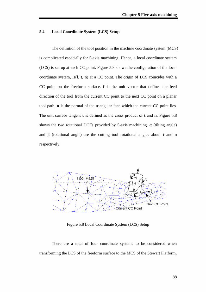
Chapter 5 Five-axis machining
88
5.4 Local Coordinate System (LCS) Setup
The definition of the tool position in the machine coordinate system (MCS)
is complicated especially for 5-axis machining. Hence, a local coordinate system
(LCS) is set up at each CC point. Figure 5.8 shows the configuration of the local
coordinate system, H(f, t, n) at a CC point. The origin of LCS coincides with a
CC point on the freeform surface. f is the unit vector that defines the feed
direction of the tool from the current CC point to the next CC point on a planar
tool path. n is the normal of the triangular face which the current CC point lies.
The unit surface tangent t is defined as the cross product of t and n. Figure 5.8
shows the two rotational DOFs provided by 5-axis machining. α (tilting angle)
and β (rotational angle) are the cutting tool rotational angles about t and n
respectively.
n
f
t
Current CC Point
Next CC Point
Tool Path
Figure 5.8 Local Coordinate System (LCS) Setup
There are a total of four coordinate systems to be considered when
transforming the LCS of the freeform surface to the MCS of the Stewart Platform,
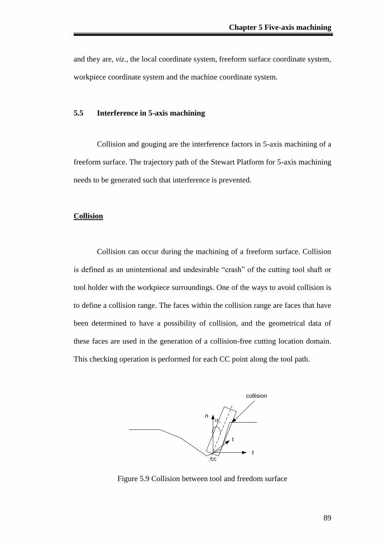
Chapter 5 Five-axis machining
89
and they are, viz., the local coordinate system, freeform surface coordinate system,
workpiece coordinate system and the machine coordinate system.
5.5 Interference in 5-axis machining
Collision and gouging are the interference factors in 5-axis machining of a
freeform surface. The trajectory path of the Stewart Platform for 5-axis machining
needs to be generated such that interference is prevented.
Collision
Collision can occur during the machining of a freeform surface. Collision
is defined as an unintentional and undesirable “crash” of the cutting tool shaft or
tool holder with the workpiece surroundings. One of the ways to avoid collision is
to define a collision range. The faces within the collision range are faces that have
been determined to have a possibility of collision, and the geometrical data of
these faces are used in the generation of a collision-free cutting location domain.
This checking operation is performed for each CC point along the tool path.
collision
t
f
nc
cc
Figure 5.9 Collision between tool and freedom surface
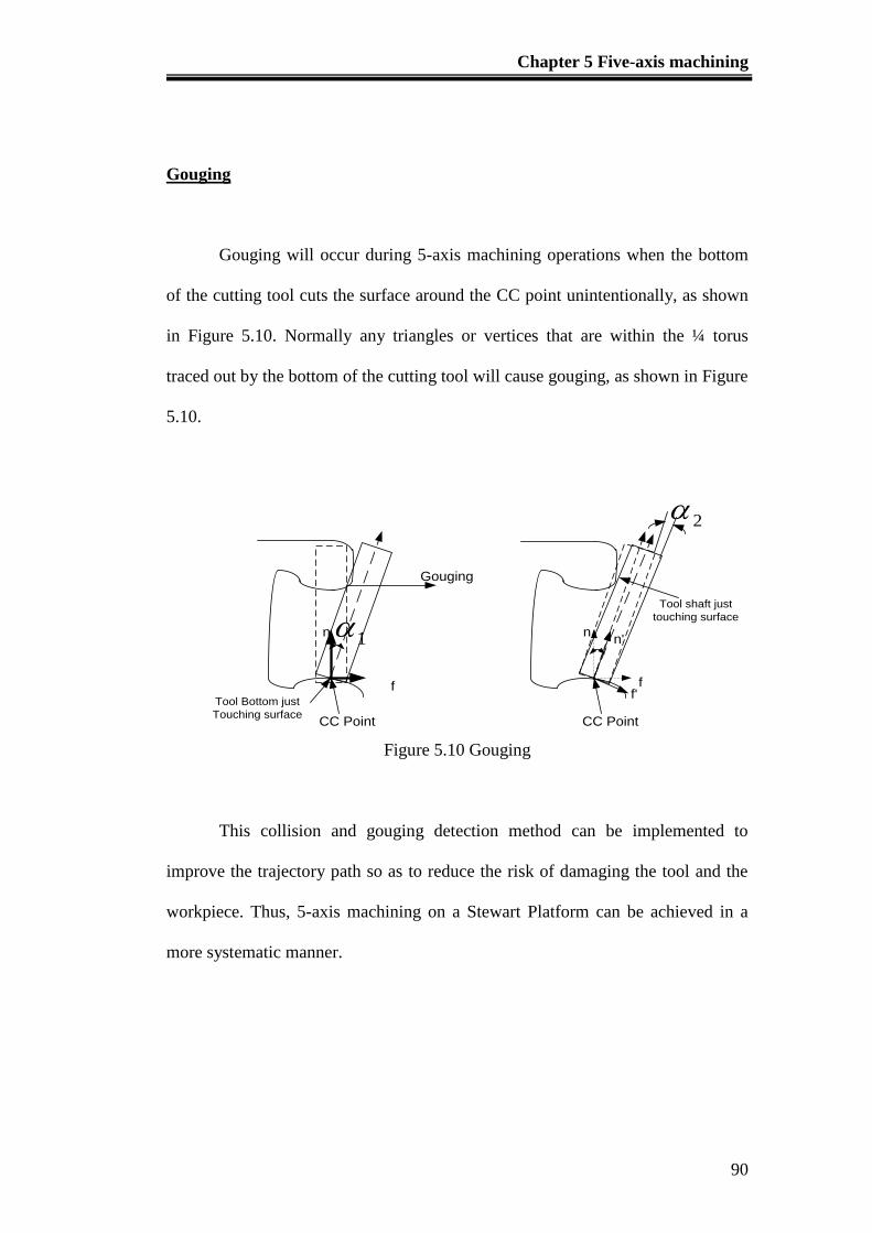
Chapter 5 Five-axis machining
90
Gouging
Gouging will occur during 5-axis machining operations when the bottom
of the cutting tool cuts the surface around the CC point unintentionally, as shown
in Figure 5.10. Normally any triangles or vertices that are within the ¼ torus
traced out by the bottom of the cutting tool will cause gouging, as shown in Figure
5.10.
Tool Bottom just
Touching surface
Gouging
n
f
1
CC Point
n
f
2
CC Point
n'
f'
Tool shaft just
touching surface
Figure 5.10 Gouging
This collision and gouging detection method can be implemented to
improve the trajectory path so as to reduce the risk of damaging the tool and the
workpiece. Thus, 5-axis machining on a Stewart Platform can be achieved in a
more systematic manner.
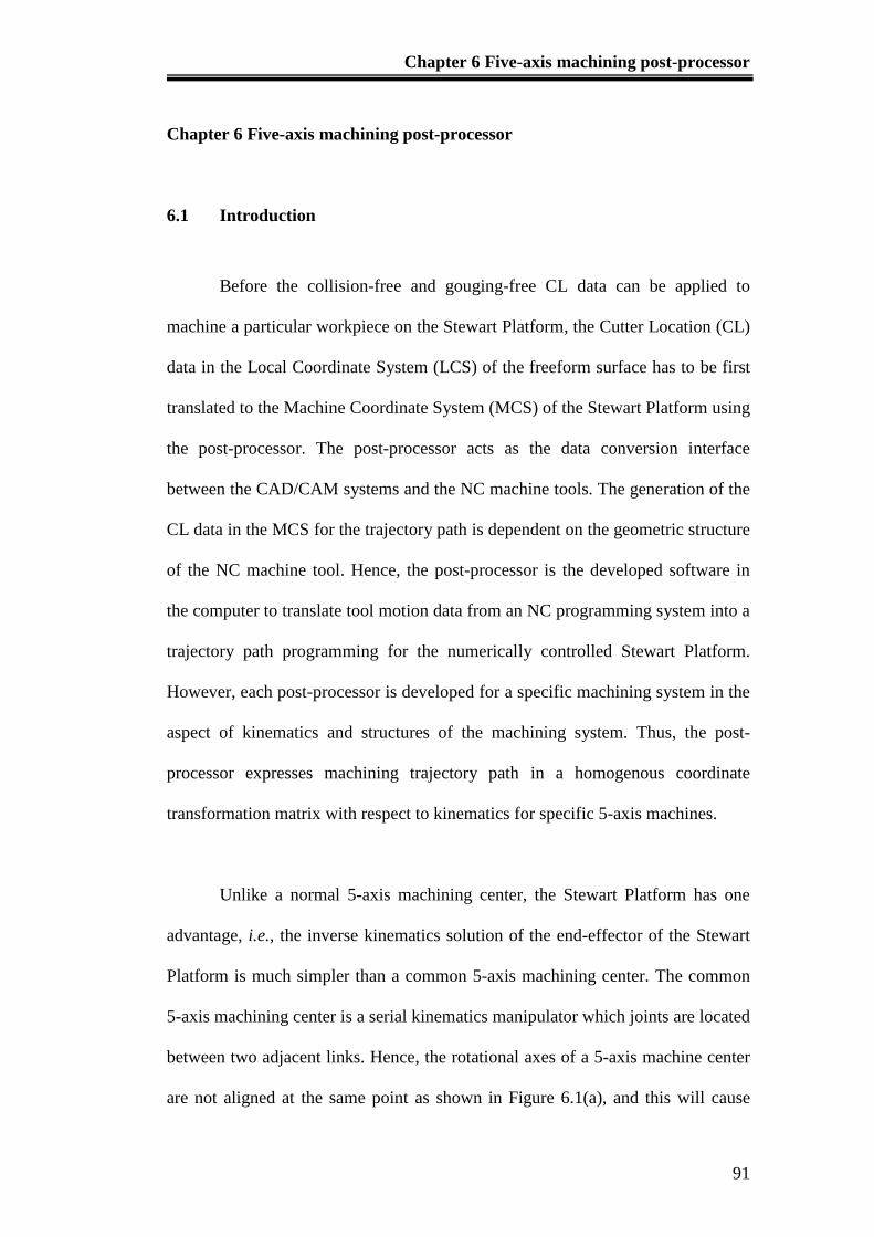
Chapter 6 Five-axis machining post-processor
91
Chapter 6 Five-axis machining post-processor
6.1 Introduction
Before the collision-free and gouging-free CL data can be applied to
machine a particular workpiece on the Stewart Platform, the Cutter Location (CL)
data in the Local Coordinate System (LCS) of the freeform surface has to be first
translated to the Machine Coordinate System (MCS) of the Stewart Platform using
the post-processor. The post-processor acts as the data conversion interface
between the CAD/CAM systems and the NC machine tools. The generation of the
CL data in the MCS for the trajectory path is dependent on the geometric structure
of the NC machine tool. Hence, the post-processor is the developed software in
the computer to translate tool motion data from an NC programming system into a
trajectory path programming for the numerically controlled Stewart Platform.
However, each post-processor is developed for a specific machining system in the
aspect of kinematics and structures of the machining system. Thus, the post-
processor expresses machining trajectory path in a homogenous coordinate
transformation matrix with respect to kinematics for specific 5-axis machines.
Unlike a normal 5-axis machining center, the Stewart Platform has one
advantage, i.e., the inverse kinematics solution of the end-effector of the Stewart
Platform is much simpler than a common 5-axis machining center. The common
5-axis machining center is a serial kinematics manipulator which joints are located
between two adjacent links. Hence, the rotational axes of a 5-axis machine center
are not aligned at the same point as shown in Figure 6.1(a), and this will cause
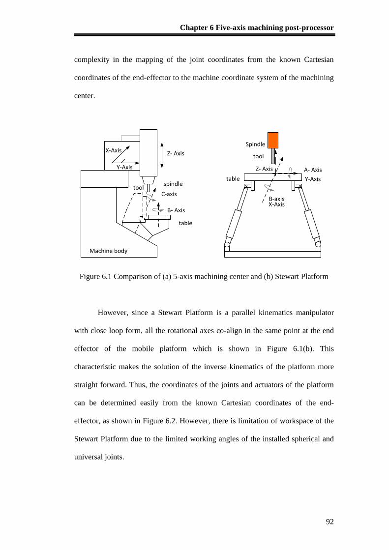
Chapter 6 Five-axis machining post-processor
92
complexity in the mapping of the joint coordinates from the known Cartesian
coordinates of the end-effector to the machine coordinate system of the machining
center.
toolspindle
B- Axis
C-axis
table
Machine body
Spindle
tool
table
A- Axis
B-axis
Z- Axis
Y-Axis
X-Axis
Y-Axis
X-Axis
Z- Axis
Figure 6.1 Comparison of (a) 5-axis machining center and (b) Stewart Platform
However, since a Stewart Platform is a parallel kinematics manipulator
with close loop form, all the rotational axes co-align in the same point at the end
effector of the mobile platform which is shown in Figure 6.1(b). This
characteristic makes the solution of the inverse kinematics of the platform more
straight forward. Thus, the coordinates of the joints and actuators of the platform
can be determined easily from the known Cartesian coordinates of the end-
effector, as shown in Figure 6.2. However, there is limitation of workspace of the
Stewart Platform due to the limited working angles of the installed spherical and
universal joints.
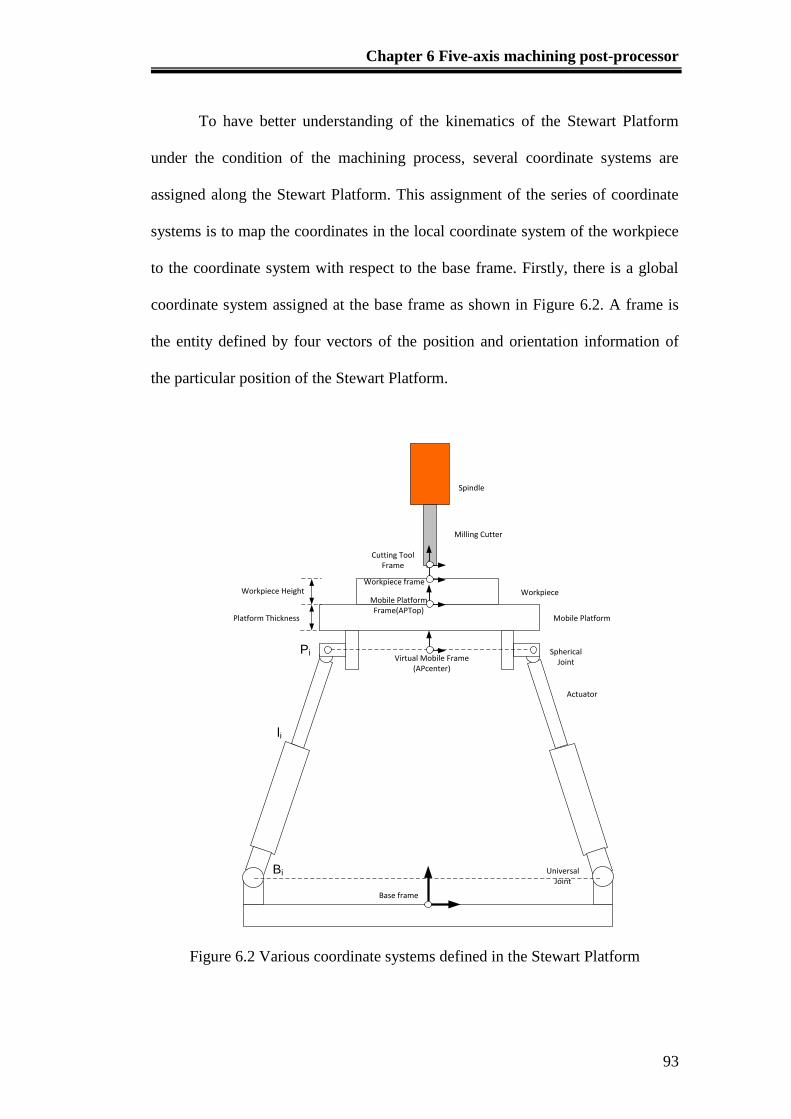
Chapter 6 Five-axis machining post-processor
93
To have better understanding of the kinematics of the Stewart Platform
under the condition of the machining process, several coordinate systems are
assigned along the Stewart Platform. This assignment of the series of coordinate
systems is to map the coordinates in the local coordinate system of the workpiece
to the coordinate system with respect to the base frame. Firstly, there is a global
coordinate system assigned at the base frame as shown in Figure 6.2. A frame is
the entity defined by four vectors of the position and orientation information of
the particular position of the Stewart Platform.
Milling Cutter
Spindle
Workpiece
Mobile Platform
Actuator
Workpiece Height
Platform Thickness
Base frame
Virtual Mobile Frame(APcenter)
Mobile Platform Frame(APTop)
Cutting Tool Frame
Universal Joint
Spherical Joint
Pi
Bi
li
Workpiece frame
Figure 6.2 Various coordinate systems defined in the Stewart Platform
Chapter 6 Five-axis machining post-processor
94
In addition, a few local coordinate systems are assigned along the mobile
platform. A virtual mobile platform coordinate system is assigned virtually at the
center point where it is coplanar with the coordinates of the spherical joints as
shown in Figure 6.2. Next, the mobile platform coordinate system is assigned at
the center of the top surface of the mobile platform while the workpiece
coordinate system is also assigned on the top surface of the workpiece. Lastly, a
cutting tool coordinate system is assigned at the bottom center of the cutting tool
tip. All the parameters of the local coordinate systems are referred to the global
coordinate system at the base frame. Since the mobile platform is a rigid body, the
local coordinate systems, such as the mobile platform coordinate system and the
virtual mobile coordinate system share the same translation vectors in term of X-,
Y- and Z-coordinates.
A post-processor is developed in this research to generate the appropriate
machining trajectory path of the Stewart Platform based on the local coordinates
of a freeform surface. Based on the equations in Chapter 2, the joint coordinates
of an actuator can be determined using Equation (6.1),
6...,2,1, iTPRP iinew (6.1)
6...,2,1, iBTPRl iii (6.2)
where R is the rotational matrix.
coscossincossin
sincoscossinsincoscossinsinsincossin
sinsincossincoscossinsinsincoscoscos
33Rot
(6.3)
and T is the translational movement of the end effector of the mobile platform.
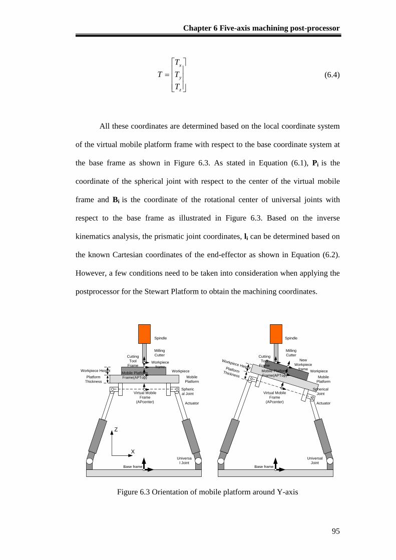
Chapter 6 Five-axis machining post-processor
95
z
y
x
T
T
T
T (6.4)
All these coordinates are determined based on the local coordinate system
of the virtual mobile platform frame with respect to the base coordinate system at
the base frame as shown in Figure 6.3. As stated in Equation (6.1), Pi is the
coordinate of the spherical joint with respect to the center of the virtual mobile
frame and Bi is the coordinate of the rotational center of universal joints with
respect to the base frame as illustrated in Figure 6.3. Based on the inverse
kinematics analysis, the prismatic joint coordinates, li can be determined based on
the known Cartesian coordinates of the end-effector as shown in Equation (6.2).
However, a few conditions need to be taken into consideration when applying the
postprocessor for the Stewart Platform to obtain the machining coordinates.
Milling
Cutter
Spindle
Workpiece
Mobile
Platform
Actuator
Workpiece Height
Platform
Thickness
Base frame
Virtual Mobile
Frame
(APcenter)
Mobile Platform
Frame(APTop)
Cutting
Tool
Frame
Universa
l Joint
Spheric
al Joint
Milling
Cutter
Spindle
Workpiece
Mobile
Platform
Actuator
Base frame
Virtual Mobile
Frame
(APcenter)
Mobile Platform
Frame(APTop)
Cutting
Tool
Frame
Universal
Joint
Spherical
Joint
Workpiece HeightPlatformThickness
Z
X
Workpiece
frame
New
Workpiece
frame
Figure 6.3 Orientation of mobile platform around Y-axis
Chapter 6 Five-axis machining post-processor
96
When the machining trajectory path of the Stewart Platform is used in 3-
axis machining, the orientation angle of the mobile platform is negligible since
only translation movement is concerned in the machining process. In addition, the
workpiece and the mobile platform can be considered as one single rigid body.
Hence, as long as the local coordinates of the workpiece are known, the
machining coordinates can be evaluated easily by implementing the translational
motion T of the Stewart Platform. However, when the Stewart Platform is
performing 5-axis machining, the rotational angles around A and B axes as shown
in Figure 6.1 will introduce different challenges to define the center coordinates of
orientation. It is because the lengths of the actuators are defined based on the
orientation and translation of the mobile platform. However, in 5-axis machining,
the respective machining coordinates are defined based on the orientation and
translation of the center of the mobile platform; now it is defined based on the
orientation and translation of the contact point between the freeform machined
workpiece and the center of the bottom point of the cutting tool.
As shown in Figure 6.3, five local coordinate systems (LCS) are defined
which can affect the joint coordinates during the movement of the Stewart
Platform in five axis machining, namely, the base frame LCS, virtual mobile
frame LCS, mobile platform frame LCS, workpiece frame LCS and the cutting
tool frame LCS. Normally, the joint coordinates of the prismatic actuators can be
determined based on the difference between the coordinates in the base frame
LCS and the coordinates in the virtual mobile frame LCS. However, in 5-axis
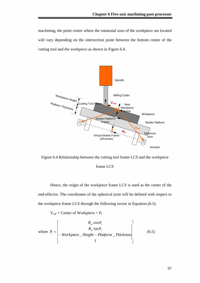
Chapter 6 Five-axis machining post-processor
97
machining, the point center where the rotational axes of the workpiece are located
will vary depending on the intersection point between the bottom center of the
cutting tool and the workpiece as shown in Figure 6.4.
Workpiece HeightPlatform Thickness
Milling Cutter
Spindle
Workpiece
Mobile Platform
Actuator
Virtual Mobile Frame
(APcenter)
Cutting Tool Frame
Spherical
Joint
Vmw
VwP
Rp
Mobile Platform
Frame
New
Workpiece
frame
Figure 6.4 Relationship between the cutting tool frame LCS and the workpiece
frame LCS
Hence, the origin of the workpiece frame LCS is used as the center of the
end-effector. The coordinates of the spherical joint will be defined with respect to
the workpiece frame LCS through the following vector in Equation (6.5).
VwP = Center of Workpiece + Pi
where
1
__
sin
cos
ThicknessPlatformHeightWorkpiece
R
R
Pip
ip
i
(6.5)
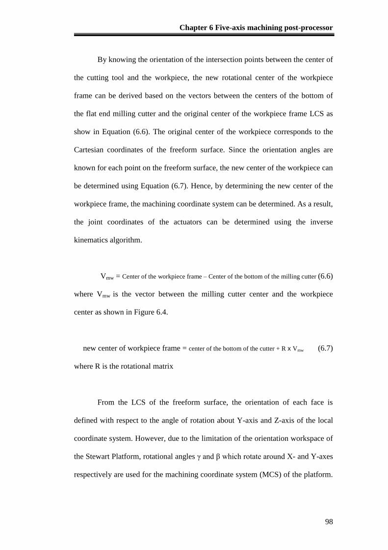
Chapter 6 Five-axis machining post-processor
98
By knowing the orientation of the intersection points between the center of
the cutting tool and the workpiece, the new rotational center of the workpiece
frame can be derived based on the vectors between the centers of the bottom of
the flat end milling cutter and the original center of the workpiece frame LCS as
show in Equation (6.6). The original center of the workpiece corresponds to the
Cartesian coordinates of the freeform surface. Since the orientation angles are
known for each point on the freeform surface, the new center of the workpiece can
be determined using Equation (6.7). Hence, by determining the new center of the
workpiece frame, the machining coordinate system can be determined. As a result,
the joint coordinates of the actuators can be determined using the inverse
kinematics algorithm.
Vmw = Center of the workpiece frame – Center of the bottom of the milling cutter (6.6)
where Vmw is the vector between the milling cutter center and the workpiece
center as shown in Figure 6.4.
new center of workpiece frame = center of the bottom of the cutter + R x Vmw (6.7)
where R is the rotational matrix
From the LCS of the freeform surface, the orientation of each face is
defined with respect to the angle of rotation about Y-axis and Z-axis of the local
coordinate system. However, due to the limitation of the orientation workspace of
the Stewart Platform, rotational angles γ and β which rotate around X- and Y-axes
respectively are used for the machining coordinate system (MCS) of the platform.
Chapter 6 Five-axis machining post-processor
99
Therefore, an algorithm is developed for the mapping of the orientation angles of
the intersected faces in the freeform surface LCS to the orientation angles of the
trajectory path in the machining coordinate system of the Stewart Platform. The
mapping process is illustrated in Figure 6.5.
X
Y
Z
z
y
x
N
N
N
Nr
βγ
Figure 6.5 Normal Vector of Face intersected with the Cutting Plane
As shown in Figure 6.5, the vectors [Nx Ny Nz] and the magnitude
222
zyxR NNNN of the normal vector of the faces intersect with the
cutting plane at the freeform surface LCS are known. Since the orientation of the
Stewart Platform is limited to rotation about the X- and Y-axes, the rotational
matrix can be further simplified as in Equation (6.8).
coscossincossin
sincos0
cossinsinsincos
xyRot (6.8)
Hence, mapping of the angles of rotation of the machining coordinate of
the Stewart Platform to the angles of rotation of the faces in the freeform surface
LCS can be defined as below.
Chapter 6 Five-axis machining post-processor
100
zr
yr
xr
z
y
x
r
NN
NN
NN
where
N
N
N
N
coscos
sin
cossin
0
0
coscossincossin
sincos0
cossinsinsincos
(6.9)
By rearranging Equation (6.9), the angle of rotation can be determined
using Equations (6.10) and (6.11). Thus, the machining coordinates can be
obtained based on the local coordinate system of the freeform surface. Hence, the
lengths of each link can be verified and the trajectory path of the Stewart Platform
can be defined for 5-axis machining.
r
y
N
N1sin (6.10)
z
x
N
N1tan (6.11)
6.2 Case Study: 5-axis surface machining
The postprocessor for converting the NC programs for 5-axis machining to
the trajectory paths for the Stewart Platform was developed in MATLAB®. Firstly,
a part to be machined is modeled using SolidWorks, and the drawing file exported
as an ASCII STL file, for example, as shown in Figure 6.6. After an STL file has
been generated, this text file is imported into MATLAB® to convert into the
corresponding faces, vertices and colors, which are recognized by MATLAB®, to
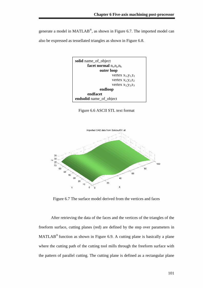
Chapter 6 Five-axis machining post-processor
101
generate a model in MATLAB®, as shown in Figure 6.7. The imported model can
also be expressed as tessellated triangles as shown in Figure 6.8.
Figure 6.6 ASCII STL text format
Figure 6.7 The surface model derived from the vertices and faces
After retrieving the data of the faces and the vertices of the triangles of the
freeform surface, cutting planes (red) are defined by the step over parameters in
MATLAB®
function as shown in Figure 6.9. A cutting plane is basically a plane
where the cutting path of the cutting tool mills through the freeform surface with
the pattern of parallel cutting. The cutting plane is defined as a rectangular plane
solid name_of_object
facet normal ni,nj,nk
outer loop
vertex x1,y1,z1
vertex x2,y2,z2
vertex x3,y3,z3
endloop
endfacet
endsolid name_of_object
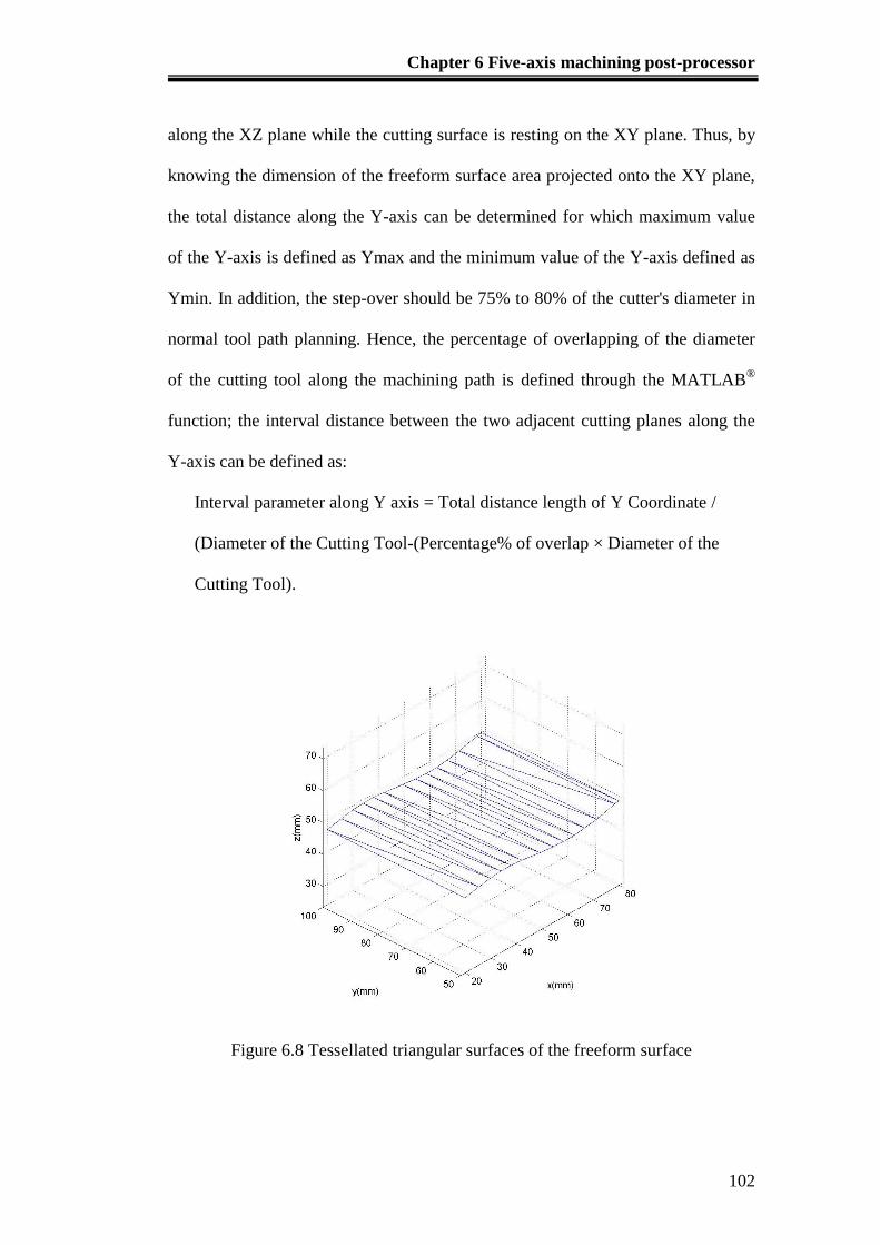
Chapter 6 Five-axis machining post-processor
102
along the XZ plane while the cutting surface is resting on the XY plane. Thus, by
knowing the dimension of the freeform surface area projected onto the XY plane,
the total distance along the Y-axis can be determined for which maximum value
of the Y-axis is defined as Ymax and the minimum value of the Y-axis defined as
Ymin. In addition, the step-over should be 75% to 80% of the cutter's diameter in
normal tool path planning. Hence, the percentage of overlapping of the diameter
of the cutting tool along the machining path is defined through the MATLAB®
function; the interval distance between the two adjacent cutting planes along the
Y-axis can be defined as:
Interval parameter along Y axis = Total distance length of Y Coordinate /
(Diameter of the Cutting Tool-(Percentage% of overlap × Diameter of the
Cutting Tool).
Figure 6.8 Tessellated triangular surfaces of the freeform surface

Chapter 6 Five-axis machining post-processor
103
Figure 6.9 Intersected points with norm (green dot line) along the cutting plane
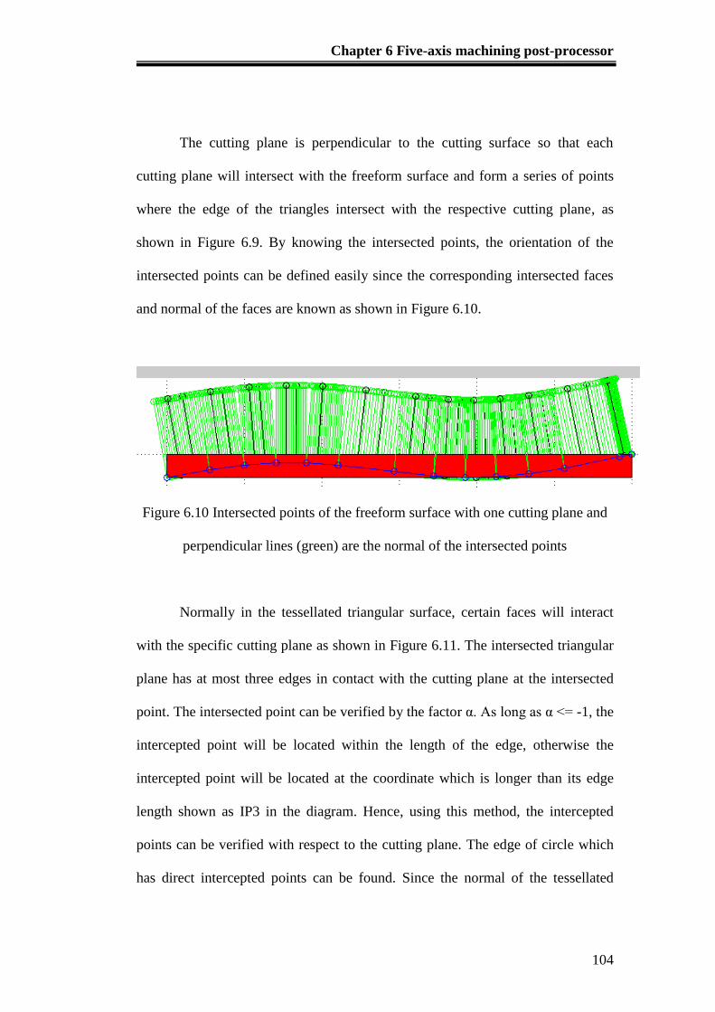
Chapter 6 Five-axis machining post-processor
104
The cutting plane is perpendicular to the cutting surface so that each
cutting plane will intersect with the freeform surface and form a series of points
where the edge of the triangles intersect with the respective cutting plane, as
shown in Figure 6.9. By knowing the intersected points, the orientation of the
intersected points can be defined easily since the corresponding intersected faces
and normal of the faces are known as shown in Figure 6.10.
Figure 6.10 Intersected points of the freeform surface with one cutting plane and
perpendicular lines (green) are the normal of the intersected points
Normally in the tessellated triangular surface, certain faces will interact
with the specific cutting plane as shown in Figure 6.11. The intersected triangular
plane has at most three edges in contact with the cutting plane at the intersected
point. The intersected point can be verified by the factor α. As long as α <= -1, the
intercepted point will be located within the length of the edge, otherwise the
intercepted point will be located at the coordinate which is longer than its edge
length shown as IP3 in the diagram. Hence, using this method, the intercepted
points can be verified with respect to the cutting plane. The edge of circle which
has direct intercepted points can be found. Since the normal of the tessellated
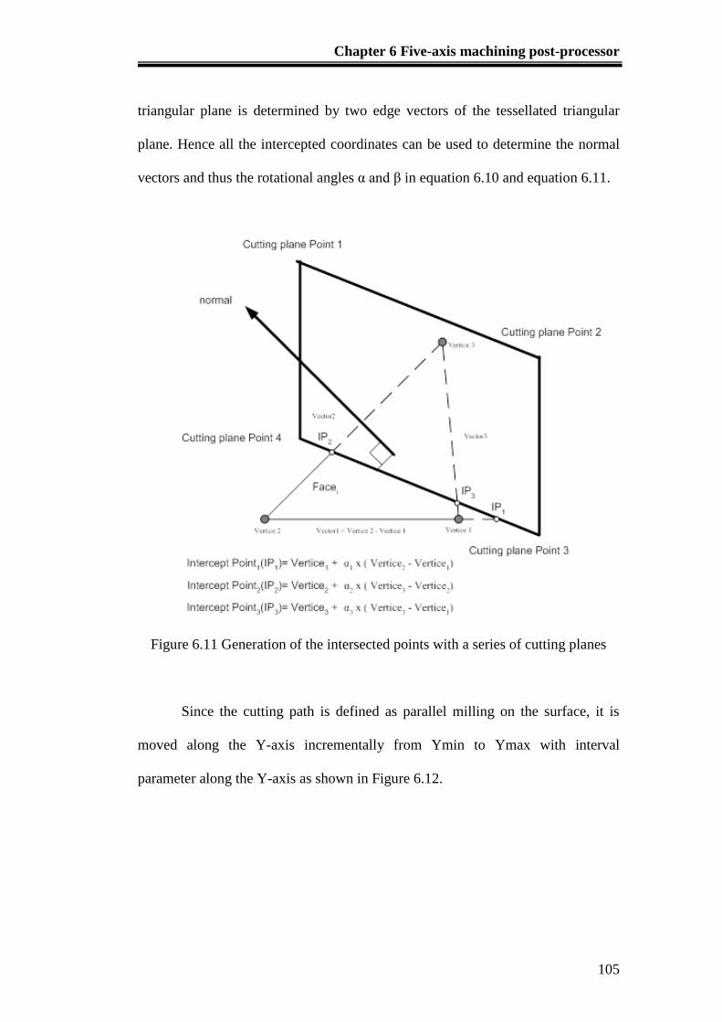
Chapter 6 Five-axis machining post-processor
105
triangular plane is determined by two edge vectors of the tessellated triangular
plane. Hence all the intercepted coordinates can be used to determine the normal
vectors and thus the rotational angles α and β in equation 6.10 and equation 6.11.
Figure 6.11 Generation of the intersected points with a series of cutting planes
Since the cutting path is defined as parallel milling on the surface, it is
moved along the Y-axis incrementally from Ymin to Ymax with interval
parameter along the Y-axis as shown in Figure 6.12.
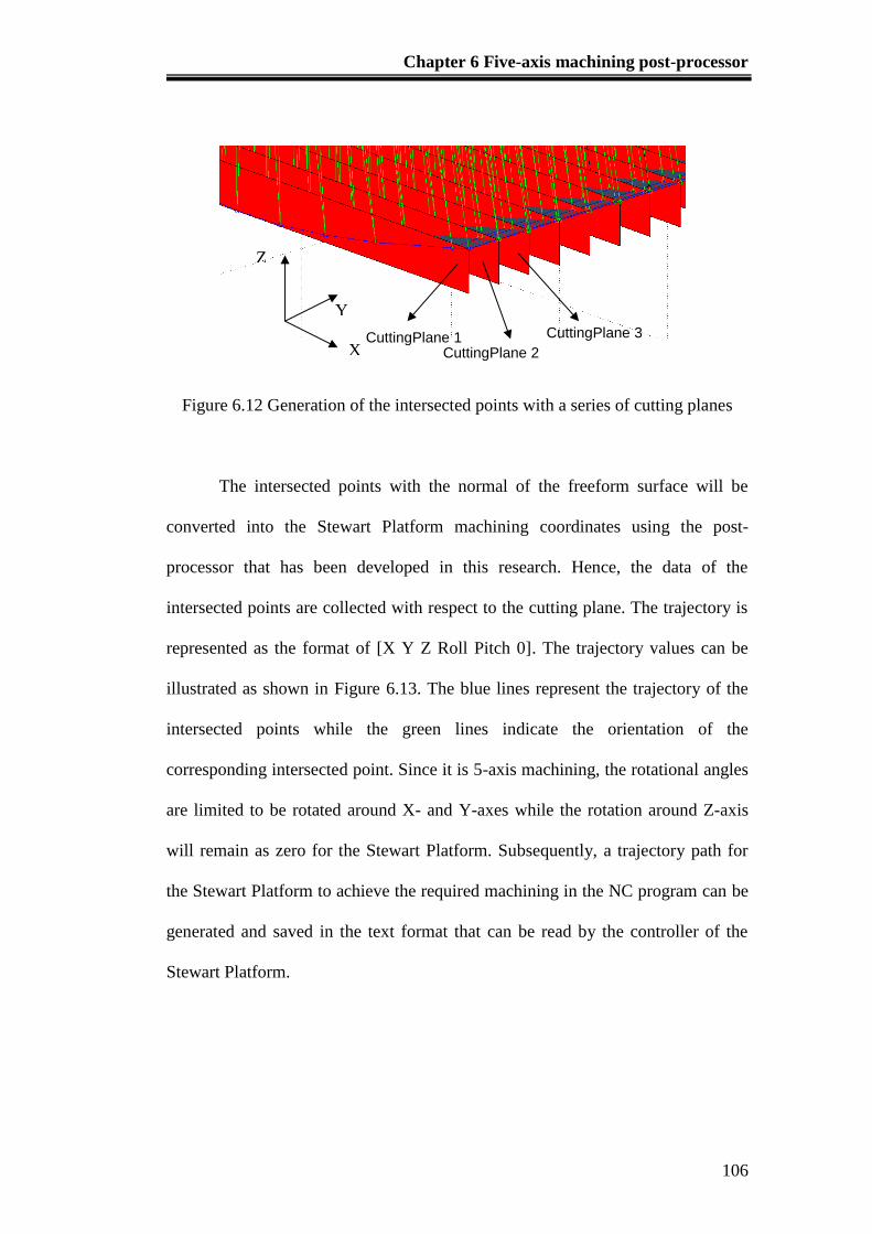
Chapter 6 Five-axis machining post-processor
106
Figure 6.12 Generation of the intersected points with a series of cutting planes
The intersected points with the normal of the freeform surface will be
converted into the Stewart Platform machining coordinates using the post-
processor that has been developed in this research. Hence, the data of the
intersected points are collected with respect to the cutting plane. The trajectory is
represented as the format of [X Y Z Roll Pitch 0]. The trajectory values can be
illustrated as shown in Figure 6.13. The blue lines represent the trajectory of the
intersected points while the green lines indicate the orientation of the
corresponding intersected point. Since it is 5-axis machining, the rotational angles
are limited to be rotated around X- and Y-axes while the rotation around Z-axis
will remain as zero for the Stewart Platform. Subsequently, a trajectory path for
the Stewart Platform to achieve the required machining in the NC program can be
generated and saved in the text format that can be read by the controller of the
Stewart Platform.
CuttingPlane 1 CuttingPlane 2
CuttingPlane 3
X
Y
Z
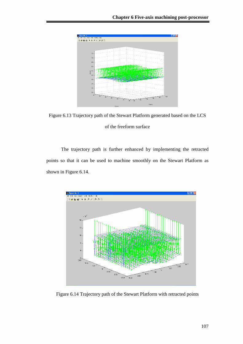
Chapter 6 Five-axis machining post-processor
107
Figure 6.13 Trajectory path of the Stewart Platform generated based on the LCS
of the freeform surface
The trajectory path is further enhanced by implementing the retracted
points so that it can be used to machine smoothly on the Stewart Platform as
shown in Figure 6.14.
Figure 6.14 Trajectory path of the Stewart Platform with retracted points
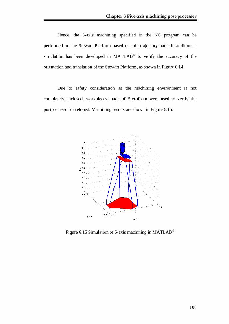
Chapter 6 Five-axis machining post-processor
108
Hence, the 5-axis machining specified in the NC program can be
performed on the Stewart Platform based on this trajectory path. In addition, a
simulation has been developed in MATLAB®
to verify the accuracy of the
orientation and translation of the Stewart Platform, as shown in Figure 6.14.
Due to safety consideration as the machining environment is not
completely enclosed, workpieces made of Styrofoam were used to verify the
postprocessor developed. Machining results are shown in Figure 6.15.
Figure 6.15 Simulation of 5-axis machining in MATLAB®
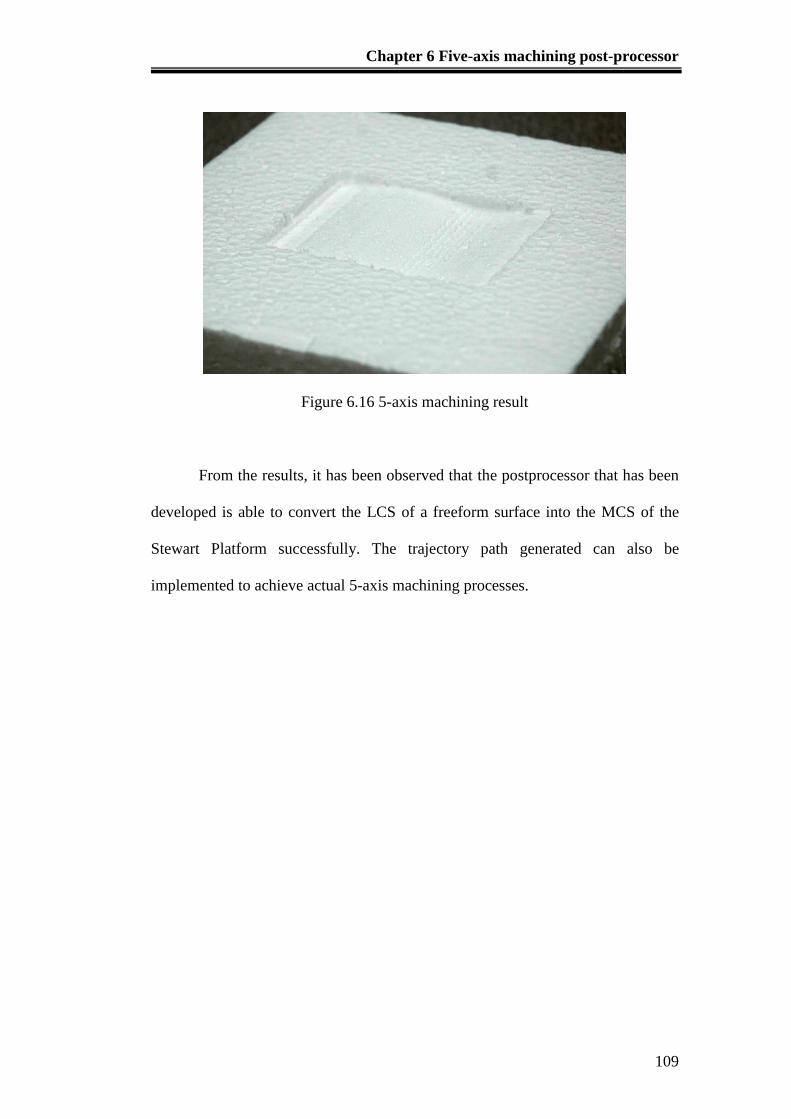
Chapter 6 Five-axis machining post-processor
109
Figure 6.16 5-axis machining result
From the results, it has been observed that the postprocessor that has been
developed is able to convert the LCS of a freeform surface into the MCS of the
Stewart Platform successfully. The trajectory path generated can also be
implemented to achieve actual 5-axis machining processes.
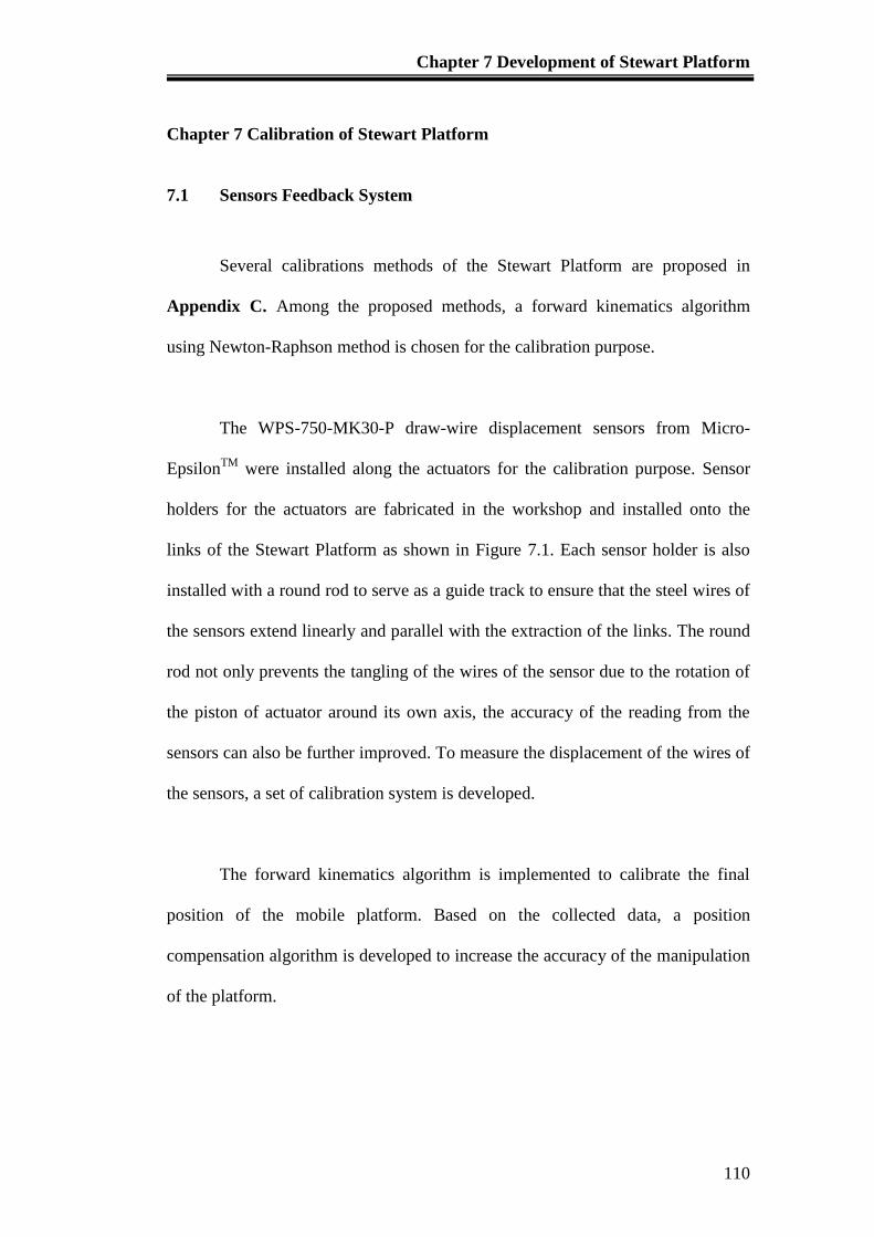
Chapter 7 Development of Stewart Platform
110
Chapter 7 Calibration of Stewart Platform
7.1 Sensors Feedback System
Several calibrations methods of the Stewart Platform are proposed in
Appendix C. Among the proposed methods, a forward kinematics algorithm
using Newton-Raphson method is chosen for the calibration purpose.
The WPS-750-MK30-P draw-wire displacement sensors from Micro-
EpsilonTM
were installed along the actuators for the calibration purpose. Sensor
holders for the actuators are fabricated in the workshop and installed onto the
links of the Stewart Platform as shown in Figure 7.1. Each sensor holder is also
installed with a round rod to serve as a guide track to ensure that the steel wires of
the sensors extend linearly and parallel with the extraction of the links. The round
rod not only prevents the tangling of the wires of the sensor due to the rotation of
the piston of actuator around its own axis, the accuracy of the reading from the
sensors can also be further improved. To measure the displacement of the wires of
the sensors, a set of calibration system is developed.
The forward kinematics algorithm is implemented to calibrate the final
position of the mobile platform. Based on the collected data, a position
compensation algorithm is developed to increase the accuracy of the manipulation
of the platform.

Chapter 7 Development of Stewart Platform
111
In addition, an offline monitoring program is developed to calibrate the
end-effector of the Stewart Platform by collecting a set of feedback data from the
wire sensors which are attached to the actuators. The collected data is used to
predict the final position of the Stewart Platform through the calculation of the
forward kinematics algorithm. Based on the result of the calibration, it is able to
calibrate the end-effector of the Stewart Platform. The forward kinematics
calibration method is better than the other calibration methods. It is able to verify
not only the position of the end-effector but also the orientation of the end-effector
(Appendix C). However, the accuracy of the result is limited by the resolution of
the wire sensor which is 0.15mm. Moreover, the fluctuation of the measured
values with wire sensors also affects the accuracy. An example is shown on the
calibration sequence of the end-effector with wire sensors in the subsequent
section.
Figure 7.1 The mounting of the sensors to the sensor holder
Holder of the
endpoint of wire of
the sensor
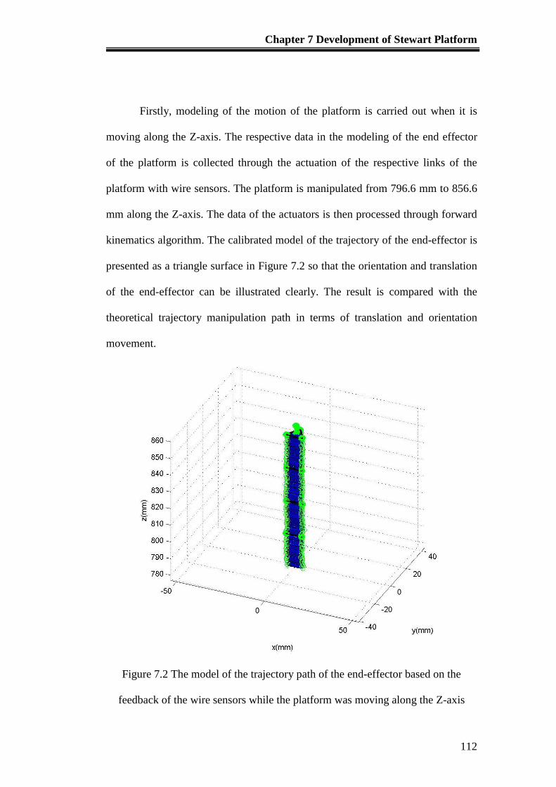
Chapter 7 Development of Stewart Platform
112
Firstly, modeling of the motion of the platform is carried out when it is
moving along the Z-axis. The respective data in the modeling of the end effector
of the platform is collected through the actuation of the respective links of the
platform with wire sensors. The platform is manipulated from 796.6 mm to 856.6
mm along the Z-axis. The data of the actuators is then processed through forward
kinematics algorithm. The calibrated model of the trajectory of the end-effector is
presented as a triangle surface in Figure 7.2 so that the orientation and translation
of the end-effector can be illustrated clearly. The result is compared with the
theoretical trajectory manipulation path in terms of translation and orientation
movement.
Figure 7.2 The model of the trajectory path of the end-effector based on the
feedback of the wire sensors while the platform was moving along the Z-axis
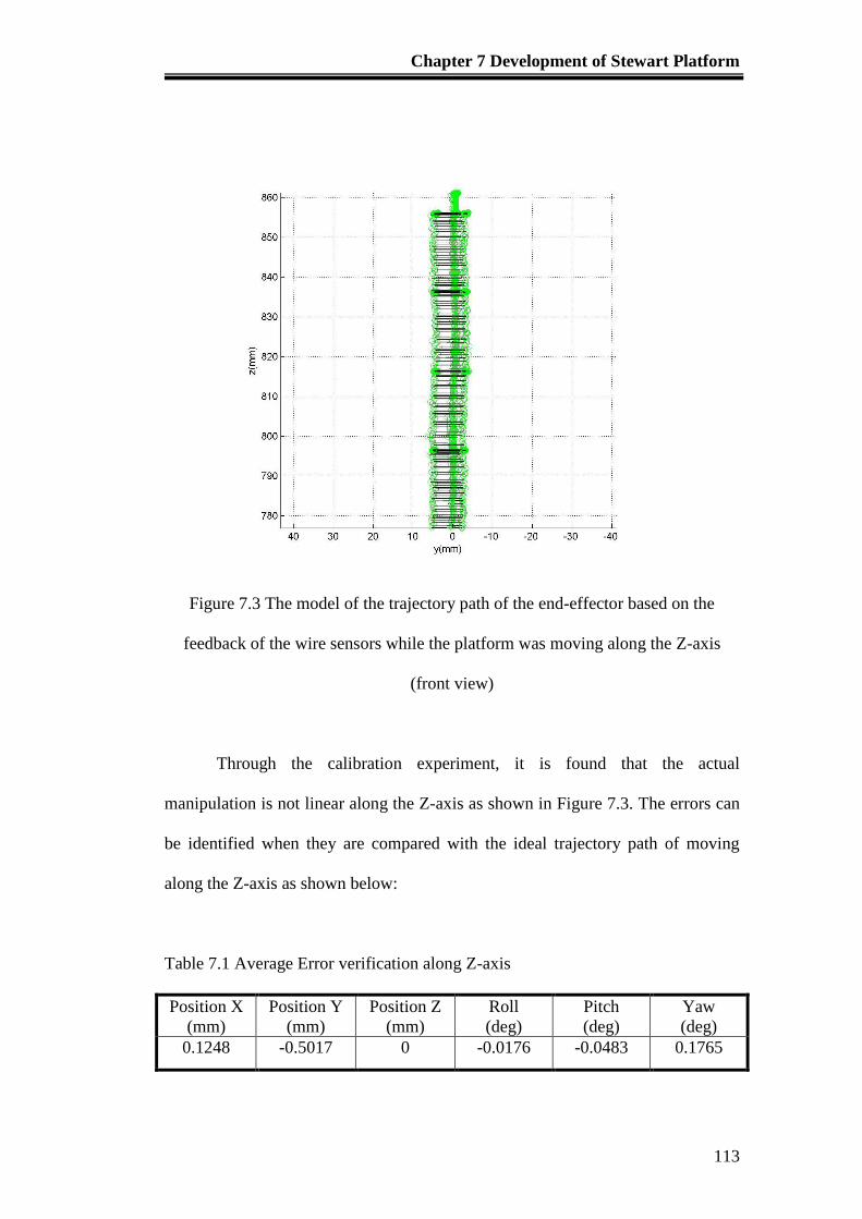
Chapter 7 Development of Stewart Platform
113
Figure 7.3 The model of the trajectory path of the end-effector based on the
feedback of the wire sensors while the platform was moving along the Z-axis
(front view)
Through the calibration experiment, it is found that the actual
manipulation is not linear along the Z-axis as shown in Figure 7.3. The errors can
be identified when they are compared with the ideal trajectory path of moving
along the Z-axis as shown below:
Table 7.1 Average Error verification along Z-axis
Position X
(mm)
Position Y
(mm)
Position Z
(mm)
Roll
(deg)
Pitch
(deg)
Yaw
(deg)
0.1248 -0.5017 0 -0.0176 -0.0483 0.1765
Chapter 7 Development of Stewart Platform
114
Besides comparing the errors between the actual and ideal trajectory paths
along the Z-axis, error verifications are also performed along the X- and Y-axes.
The Stewart Platform is manipulated to move along the X-axis from 0 to 50 mm
while other parameters are set as constant theoretically, such as Z = 856 mm and
Y = 0 mm as illustrated in Figure 7.4.
Figure 7.4 The model of the trajectory path of the end-effector based on the
feedback of the wire sensors while the platform was moving along the X-axis
Through feedback of the wire sensors, the actual position of the Stewart
Platform is determined. It is found that the motion is not even and tends to move
in a curved shape as shown in Figure 7.4. The errors can be identified as shown in
Table 7.2.
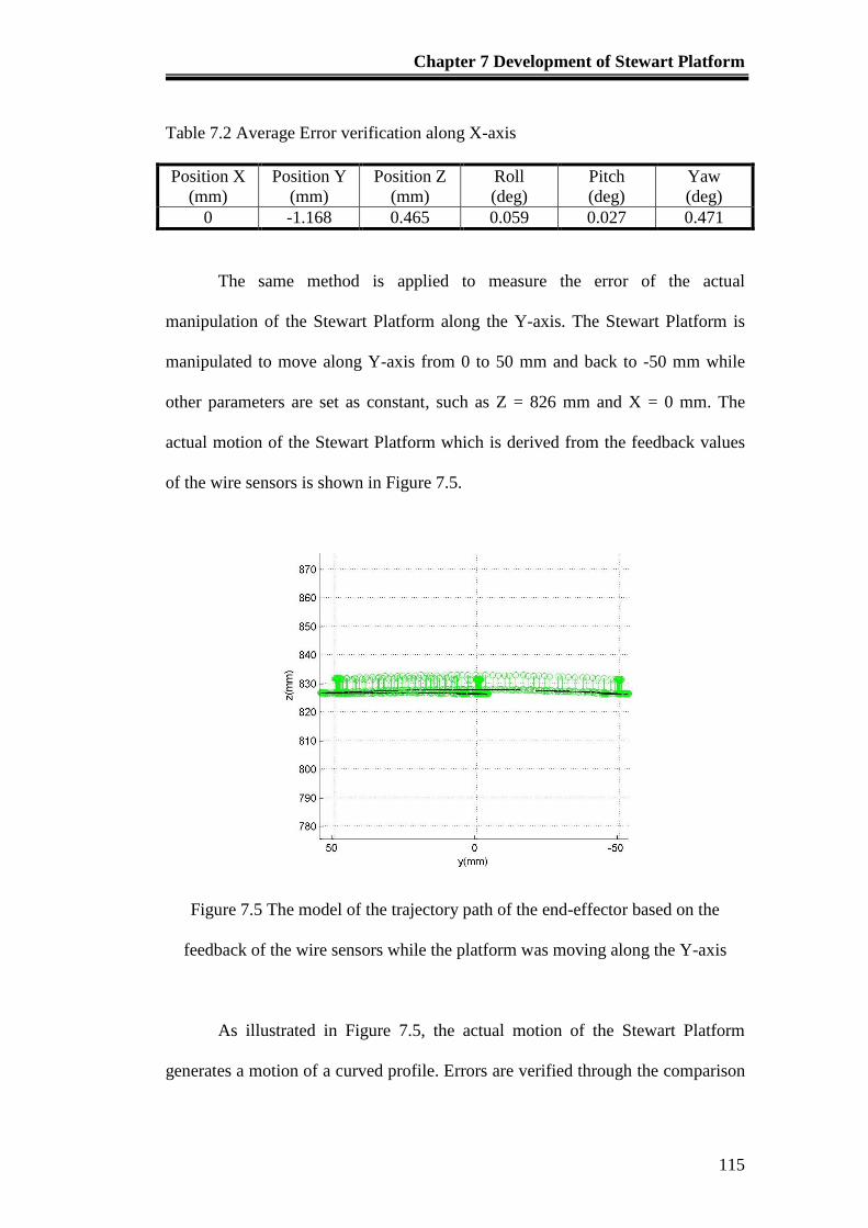
Chapter 7 Development of Stewart Platform
115
Table 7.2 Average Error verification along X-axis
Position X
(mm)
Position Y
(mm)
Position Z
(mm)
Roll
(deg)
Pitch
(deg)
Yaw
(deg)
0 -1.168 0.465 0.059 0.027 0.471
The same method is applied to measure the error of the actual
manipulation of the Stewart Platform along the Y-axis. The Stewart Platform is
manipulated to move along Y-axis from 0 to 50 mm and back to -50 mm while
other parameters are set as constant, such as Z = 826 mm and X = 0 mm. The
actual motion of the Stewart Platform which is derived from the feedback values
of the wire sensors is shown in Figure 7.5.
Figure 7.5 The model of the trajectory path of the end-effector based on the
feedback of the wire sensors while the platform was moving along the Y-axis
As illustrated in Figure 7.5, the actual motion of the Stewart Platform
generates a motion of a curved profile. Errors are verified through the comparison
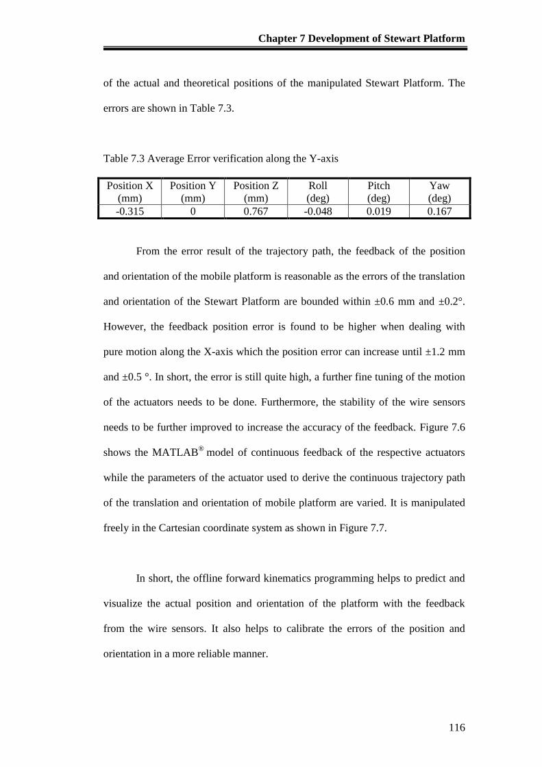
Chapter 7 Development of Stewart Platform
116
of the actual and theoretical positions of the manipulated Stewart Platform. The
errors are shown in Table 7.3.
Table 7.3 Average Error verification along the Y-axis
Position X
(mm)
Position Y
(mm)
Position Z
(mm)
Roll
(deg)
Pitch
(deg)
Yaw
(deg)
-0.315 0 0.767 -0.048 0.019 0.167
From the error result of the trajectory path, the feedback of the position
and orientation of the mobile platform is reasonable as the errors of the translation
and orientation of the Stewart Platform are bounded within ±0.6 mm and ±0.2°.
However, the feedback position error is found to be higher when dealing with
pure motion along the X-axis which the position error can increase until ±1.2 mm
and ±0.5 °. In short, the error is still quite high, a further fine tuning of the motion
of the actuators needs to be done. Furthermore, the stability of the wire sensors
needs to be further improved to increase the accuracy of the feedback. Figure 7.6
shows the MATLAB®
model of continuous feedback of the respective actuators
while the parameters of the actuator used to derive the continuous trajectory path
of the translation and orientation of mobile platform are varied. It is manipulated
freely in the Cartesian coordinate system as shown in Figure 7.7.
In short, the offline forward kinematics programming helps to predict and
visualize the actual position and orientation of the platform with the feedback
from the wire sensors. It also helps to calibrate the errors of the position and
orientation in a more reliable manner.
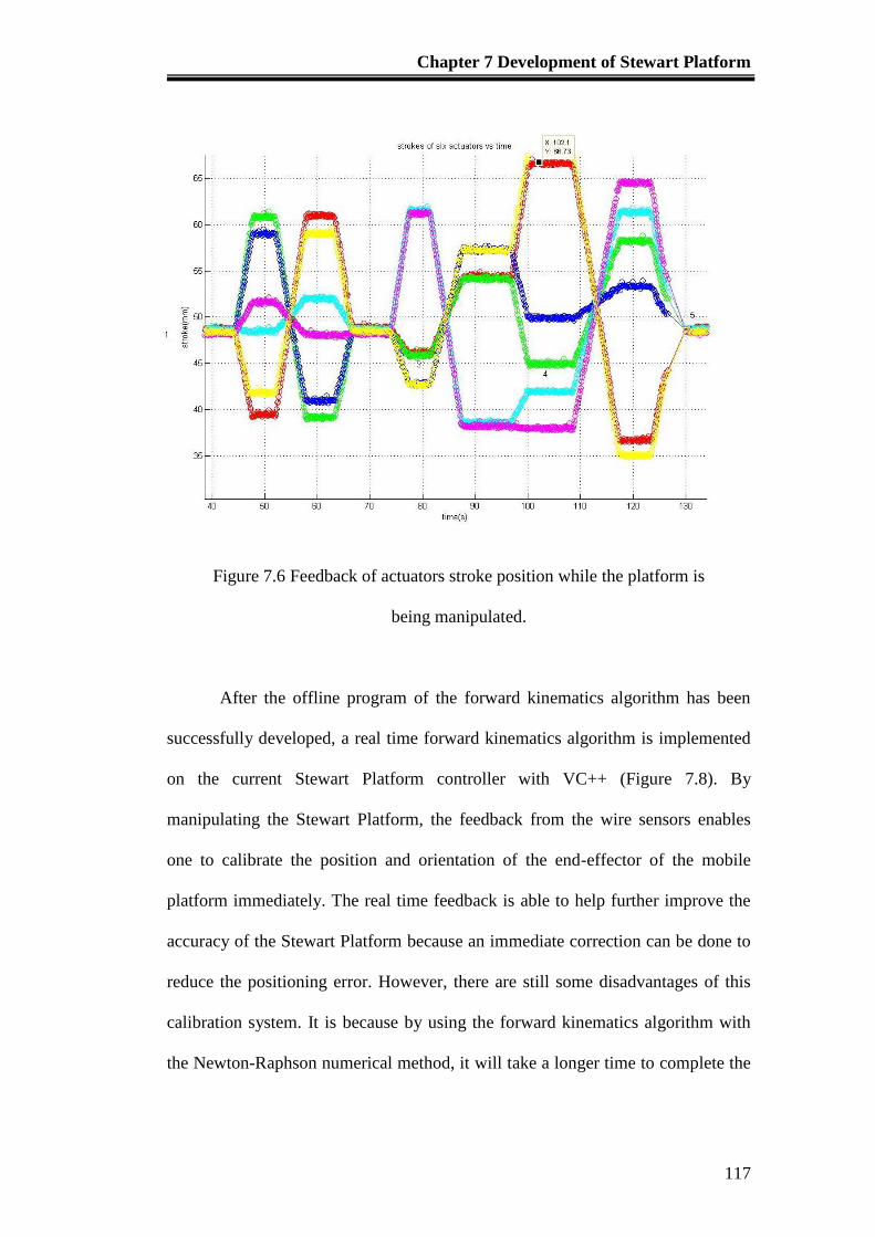
Chapter 7 Development of Stewart Platform
117
Figure 7.6 Feedback of actuators stroke position while the platform is
being manipulated.
After the offline program of the forward kinematics algorithm has been
successfully developed, a real time forward kinematics algorithm is implemented
on the current Stewart Platform controller with VC++ (Figure 7.8). By
manipulating the Stewart Platform, the feedback from the wire sensors enables
one to calibrate the position and orientation of the end-effector of the mobile
platform immediately. The real time feedback is able to help further improve the
accuracy of the Stewart Platform because an immediate correction can be done to
reduce the positioning error. However, there are still some disadvantages of this
calibration system. It is because by using the forward kinematics algorithm with
the Newton-Raphson numerical method, it will take a longer time to complete the
Chapter 7 Development of Stewart Platform
118
iterations before the final calibration can be retrieved. Furthermore, the resolution
of the wire sensors is limited to 0.15 mm but the resolution of the actuator is 0.1
mm. Thus, the retrieved data will fluctuate and are not reliable when the actuator
is commanded to be moved in interval of less than 0.1 mm. A sampling averaging
is performed which will delay the output of the position and orientation of the
platform. Hence, the current calibration system can only be considered as a near
real time calibration system.
Figure 7.7 The corresponding position and orientation of the platform end-effector
with respect to the strokes of the actuators
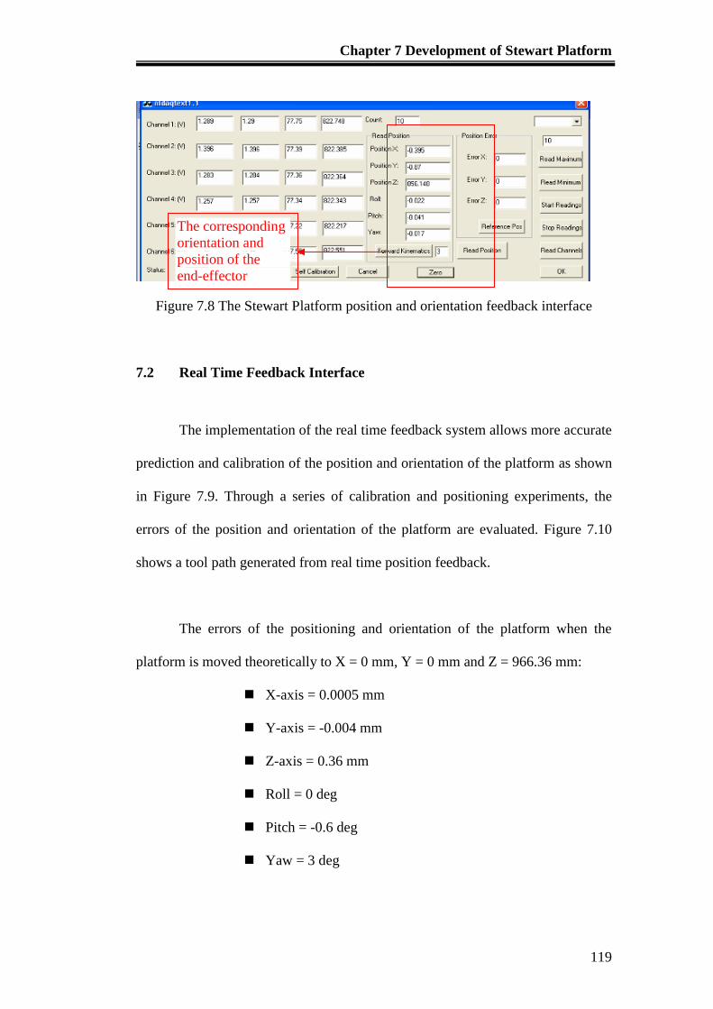
Chapter 7 Development of Stewart Platform
119
Figure 7.8 The Stewart Platform position and orientation feedback interface
7.2 Real Time Feedback Interface
The implementation of the real time feedback system allows more accurate
prediction and calibration of the position and orientation of the platform as shown
in Figure 7.9. Through a series of calibration and positioning experiments, the
errors of the position and orientation of the platform are evaluated. Figure 7.10
shows a tool path generated from real time position feedback.
The errors of the positioning and orientation of the platform when the
platform is moved theoretically to X = 0 mm, Y = 0 mm and Z = 966.36 mm:
X-axis = 0.0005 mm
Y-axis = -0.004 mm
Z-axis = 0.36 mm
Roll = 0 deg
Pitch = -0.6 deg
Yaw = 3 deg
The corresponding
orientation and
position of the
end-effector
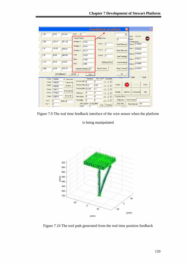
Chapter 7 Development of Stewart Platform
120
Figure 7.9 The real time feedback interface of the wire sensor when the platform
is being manipulated
Figure 7.10 The tool path generated from the real time position feedback
Feedback position
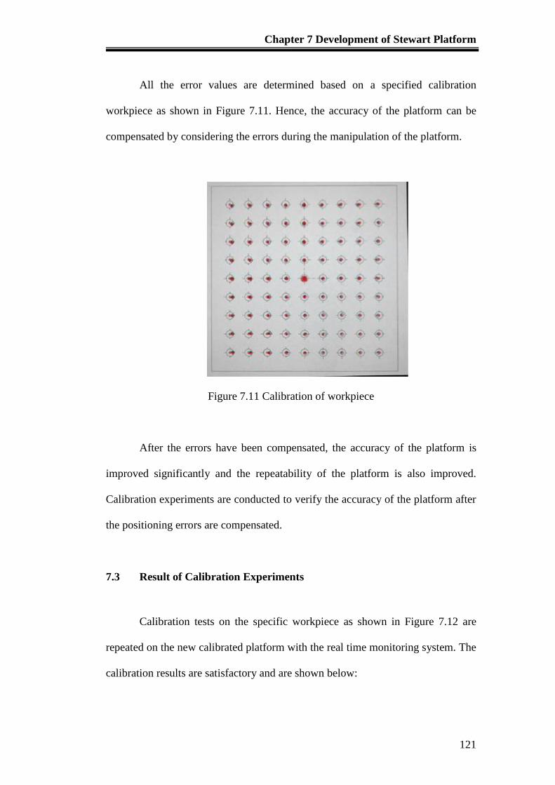
Chapter 7 Development of Stewart Platform
121
All the error values are determined based on a specified calibration
workpiece as shown in Figure 7.11. Hence, the accuracy of the platform can be
compensated by considering the errors during the manipulation of the platform.
Figure 7.11 Calibration of workpiece
After the errors have been compensated, the accuracy of the platform is
improved significantly and the repeatability of the platform is also improved.
Calibration experiments are conducted to verify the accuracy of the platform after
the positioning errors are compensated.
7.3 Result of Calibration Experiments
Calibration tests on the specific workpiece as shown in Figure 7.12 are
repeated on the new calibrated platform with the real time monitoring system. The
calibration results are satisfactory and are shown below:
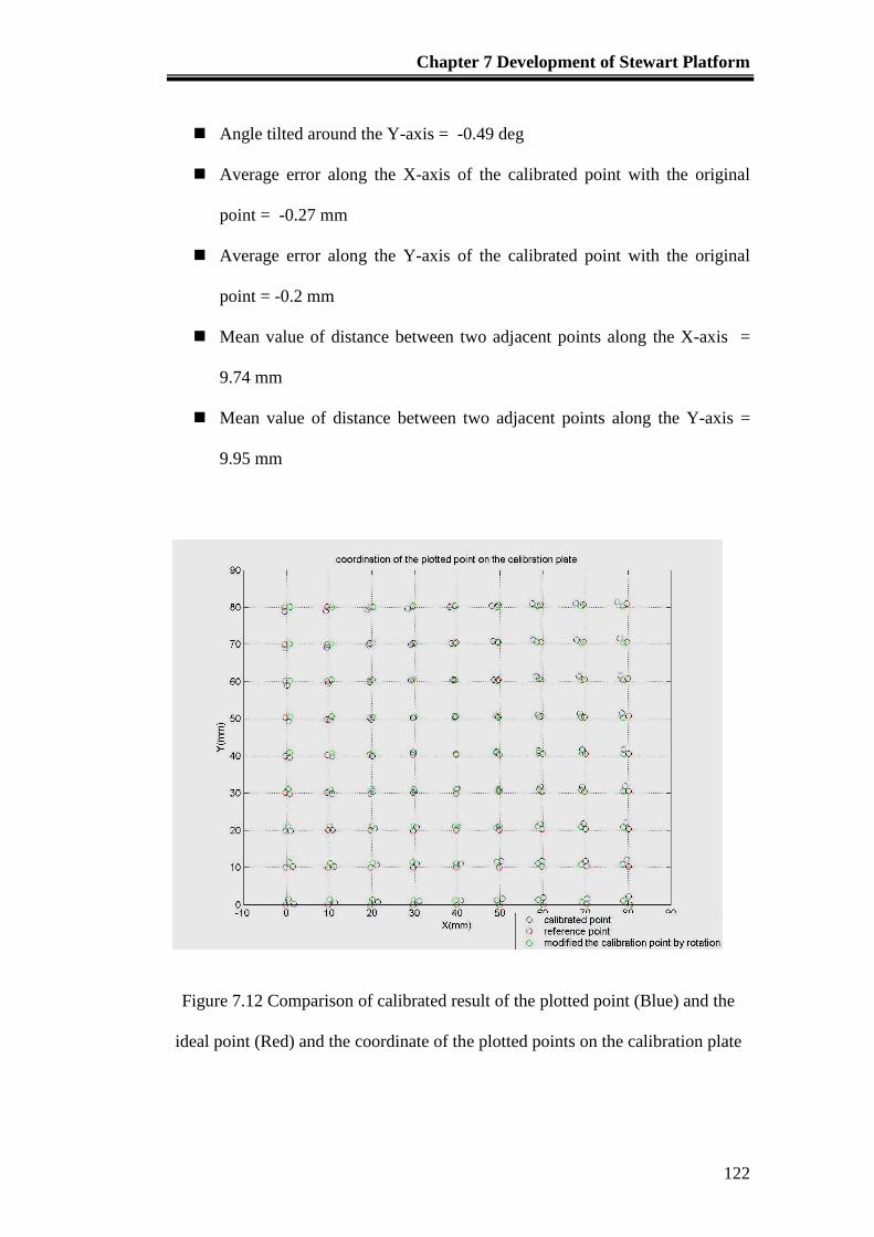
Chapter 7 Development of Stewart Platform
122
Angle tilted around the Y-axis = -0.49 deg
Average error along the X-axis of the calibrated point with the original
point = -0.27 mm
Average error along the Y-axis of the calibrated point with the original
point = -0.2 mm
Mean value of distance between two adjacent points along the X-axis =
9.74 mm
Mean value of distance between two adjacent points along the Y-axis =
9.95 mm
Figure 7.12 Comparison of calibrated result of the plotted point (Blue) and the
ideal point (Red) and the coordinate of the plotted points on the calibration plate

Chapter 7 Development of Stewart Platform
123
From the calibration results shown in Appendix D, the accuracy has been
improved significantly but there are still errors in terms of the X- and Y-axes.
From the trend of the errors, it is observed to be a linear error. Basic image
processing is developed to improve the error as shown in Appendix D. However,
the accuracy of the calibration is also limited by the resolution of the wire sensors
as discussed before.
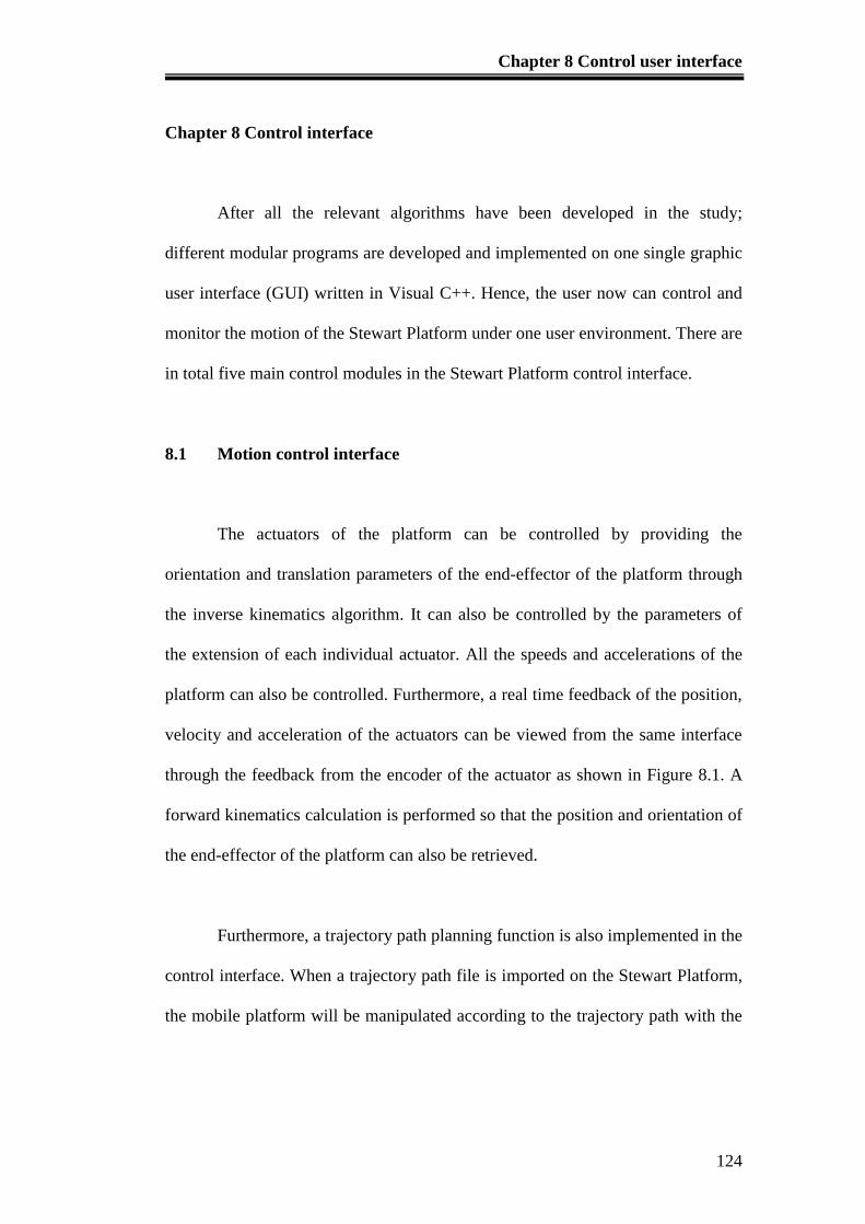
Chapter 8 Control user interface
124
Chapter 8 Control interface
After all the relevant algorithms have been developed in the study;
different modular programs are developed and implemented on one single graphic
user interface (GUI) written in Visual C++. Hence, the user now can control and
monitor the motion of the Stewart Platform under one user environment. There are
in total five main control modules in the Stewart Platform control interface.
8.1 Motion control interface
The actuators of the platform can be controlled by providing the
orientation and translation parameters of the end-effector of the platform through
the inverse kinematics algorithm. It can also be controlled by the parameters of
the extension of each individual actuator. All the speeds and accelerations of the
platform can also be controlled. Furthermore, a real time feedback of the position,
velocity and acceleration of the actuators can be viewed from the same interface
through the feedback from the encoder of the actuator as shown in Figure 8.1. A
forward kinematics calculation is performed so that the position and orientation of
the end-effector of the platform can also be retrieved.
Furthermore, a trajectory path planning function is also implemented in the
control interface. When a trajectory path file is imported on the Stewart Platform,
the mobile platform will be manipulated according to the trajectory path with the
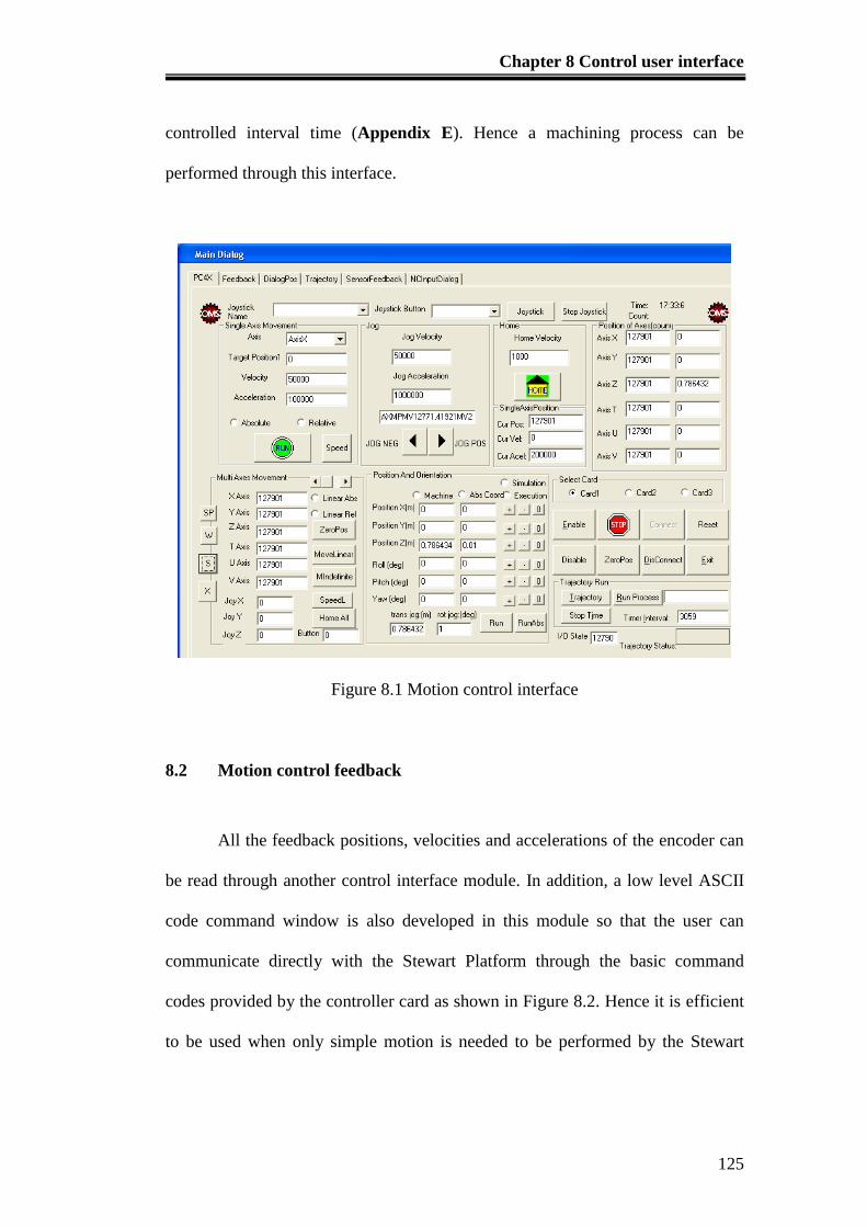
Chapter 8 Control user interface
125
controlled interval time (Appendix E). Hence a machining process can be
performed through this interface.
Figure 8.1 Motion control interface
8.2 Motion control feedback
All the feedback positions, velocities and accelerations of the encoder can
be read through another control interface module. In addition, a low level ASCII
code command window is also developed in this module so that the user can
communicate directly with the Stewart Platform through the basic command
codes provided by the controller card as shown in Figure 8.2. Hence it is efficient
to be used when only simple motion is needed to be performed by the Stewart

Chapter 8 Control user interface
126
Platform. In addition, this direct communication is also able to reduce the
communication time between the user and the Stewart Platform.
Figure 8.2 Motion control feedback
8.3 Wire sensor interface
By implementing the wire sensors interface in the GUI as shown in Figure
8.3, external sensors can be used to measure the linear motion of the actuators of
the platform which could provide a more reliable feedback. Through the feedback
of the length of the stroke of the actuator, reliable feedback of the position and
orientation of the mobile platform can be calculated through the forward
kinematics algorithm. Hence, this interface is created in the GUI to read the data
generated by the external sensors transferred in real time.
ASCII Command Windows
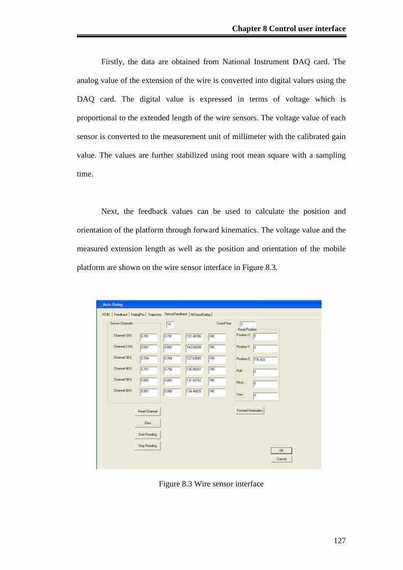
Chapter 8 Control user interface
127
Firstly, the data are obtained from National Instrument DAQ card. The
analog value of the extension of the wire is converted into digital values using the
DAQ card. The digital value is expressed in terms of voltage which is
proportional to the extended length of the wire sensors. The voltage value of each
sensor is converted to the measurement unit of millimeter with the calibrated gain
value. The values are further stabilized using root mean square with a sampling
time.
Next, the feedback values can be used to calculate the position and
orientation of the platform through forward kinematics. The voltage value and the
measured extension length as well as the position and orientation of the mobile
platform are shown on the wire sensor interface in Figure 8.3.
Figure 8.3 Wire sensor interface
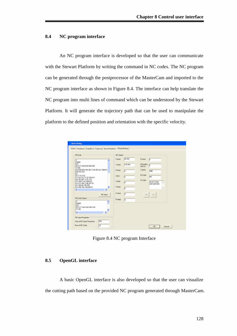
Chapter 8 Control user interface
128
8.4 NC program interface
An NC program interface is developed so that the user can communicate
with the Stewart Platform by writing the command in NC codes. The NC program
can be generated through the postprocessor of the MasterCam and imported to the
NC program interface as shown in Figure 8.4. The interface can help translate the
NC program into multi lines of command which can be understood by the Stewart
Platform. It will generate the trajectory path that can be used to manipulate the
platform to the defined position and orientation with the specific velocity.
Figure 8.4 NC program Interface
8.5 OpenGL interface
A basic OpenGL interface is also developed so that the user can visualize
the cutting path based on the provided NC program generated through MasterCam.

Chapter 8 Control user interface
129
Hence when the NC programs are imported to the NC program interface, the
conversion to the Stewart Platform machining path, the coordinates of the
trajectory path will be visualized on the window in the OpenGL interface as
shown in Figure 8.5. This function can help the user identify the error of the
trajectory path through the illustrated diagram of the platform.
Figure 8.5 OpenGL Interface
In short, the development of the graphic user interface (GUI) is able to
help the users have a friendlier working environment to control and manipulate
the Stewart Platform in machining processes. A real time feedback system
developed for the platform also helps to improve the accuracy of the system in the
aspect of translation and orientation of the mobile platform.
Chapter 9 3-DOF modular micro Parallel Kinematic Manipulator for machining
130
Chapter 9 3-DOF modular micro Parallel Kinematic Manipulator for
machining
9.1 Introduction
The increasing demand of product quality, reducing product cost and
shortening the product development cycle results in a continuing need to achieve
improvements in speed, versatility and accuracy in machining operations
especially high speed machining. Hence, the recent trends towards high speed
machining have driven the motivation in the research and development of new
novel types of parallel kinematics machines (PKMs) [Sameer, 2003].
In the process of research and development, there are still some
disadvantages of the Stewart Platform. This six-legged manipulator suffers the
disadvantages of the complex solution of direct kinematics, coupled problems of
the position and orientation movement as well as the expensive cost to
manufacture high precision spherical joint [Tsai, 1996]. Thus, further research
was performed after investigating the present Stewart Platform. A new trend of
development of the Parallel Kinematics Manipulator tends to reduce the 6-DOFs
to 3-DOFs PKMs. The reducing of DOF of the PKMs has advantages in
workspace and cost reduction. It is because 6-DOFs are not often required in
machine tools and other applications. However, the 3-DOF Parallel Kinematics
Platform provides less rigidity and degrees of freedom.
Chapter 9 3-DOF modular micro Parallel Kinematic Manipulator for machining
131
To overcome the above shortcomings, parallel manipulators with fewer
than six DOFs have been investigated. For examples, Clavel [Clavel, 1988] and
Sternheim [Sternheim, 1987] studied a 4-DOF high speed robot called Delta
Robot. Lee and Shah [Lee, 1987] analyzed a 3-DOF parallel manipulator.
Although, these two robots possess closed-form direct kinematics solutions, the
Delta robot contains twelve spherical joints while Lee and Shah’s manipulator
contains three spherical joints. In addition, the position and orientation of Lee and
Shah’s manipulator are coupled. Some 3-DOF parallel manipulator architectures
provide pure relative rotation of the moving platform about a fixed point and are
used as pointing devices, wrists of manipulators and orienting devices [Asada,
1985], [Gosselin, 1994]. Tsai [Tsai, 1996] introduced a novel 3-DOF translational
platform that is made up of only revolute joints. It performs pure translational
motion and has a closed-form solution for the direct and inverse kinematics.
Hence, a study of running 3-axis machining with the multi-axis robots
reported that it is highly unjustified as several of the axes remain under-utilized
because of the redundancy in DOF thus increases the complexity and cost. It is
because a pure 3-DOF translational or orientation motion would require the
activation of all the six-module legs, which means increase in energy consumption
[Mircea, 2002]. Hence, in terms of cost and complexity, 3-DOF 3-legged Micro
Parallel Kinematic Manipulator is cost effective and the kinematics of the
mechanism is further simplified for the purpose of control. However, if the new
system is decided to be constructed, the design algorithms either do not exist or
are very complicated.
Chapter 9 3-DOF modular micro Parallel Kinematic Manipulator for machining
132
To further increase the flexibility and functionality of the self-fabricated
Micro Stewart Platform, the concept of modular methodology is introduced. In
recent years, modular robots were increasingly proposed as means to develop
reconfigurable and self-repairable robotic systems [Mckee, 1999]. To further
optimize the performance of the 3-legged 3-DOF Parallel Manipulator and the
self-repair ability, the manipulation systems need to incorporate modularity and
self-reconfiguration capabilities. Modular robots develop many autonomous units
or modules that can be reconfigured into a huge number of designs. Ideally, the
modules will be uniform, and self-contained. The robot can change from one
configuration to another manually or automatically. Hence, a modular manipulator
can be reconfigured or modified in shape to adapt to a new environment. Modules
must interact with one another and cooperate in order to realize self-configuration.
In addition, modular Micro Parallel Kinematic Manipulators can repair
themselves by removing and replacing failed modules. Since one self-
reconfigurable modular robot can provide the functionality of many traditional
mechanisms, they will especially suit high variety tasks, such as the high speed
machining [Sameer, 2003] in the precision engineering industry.
Basically the direction of the development of the Micro Parallel Kinematic
Manipulator (MSP) is set to emphasize on the minimization of the dimensions of
the system and the portability of the system on the CNC machine.
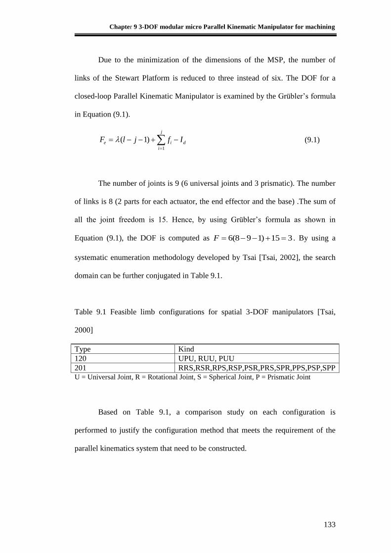
Chapter 9 3-DOF modular micro Parallel Kinematic Manipulator for machining
133
Due to the minimization of the dimensions of the MSP, the number of
links of the Stewart Platform is reduced to three instead of six. The DOF for a
closed-loop Parallel Kinematic Manipulator is examined by the Grübler’s formula
in Equation (9.1).
j
i
die IfjlF1
)1( (9.1)
The number of joints is 9 (6 universal joints and 3 prismatic). The number
of links is 8 (2 parts for each actuator, the end effector and the base) .The sum of
all the joint freedom is 15. Hence, by using Grübler’s formula as shown in
Equation (9.1), the DOF is computed as 315)198(6 F . By using a
systematic enumeration methodology developed by Tsai [Tsai, 2002], the search
domain can be further conjugated in Table 9.1.
Table 9.1 Feasible limb configurations for spatial 3-DOF manipulators [Tsai,
2000]
Type Kind
120 UPU, RUU, PUU
201 RRS,RSR,RPS,RSP,PSR,PRS,SPR,PPS,PSP,SPP U = Universal Joint, R = Rotational Joint, S = Spherical Joint, P = Prismatic Joint
Based on Table 9.1, a comparison study on each configuration is
performed to justify the configuration method that meets the requirement of the
parallel kinematics system that need to be constructed.
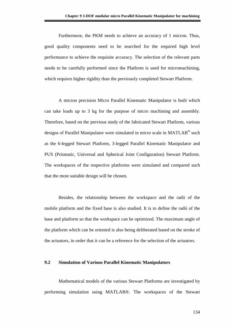
Chapter 9 3-DOF modular micro Parallel Kinematic Manipulator for machining
134
Furthermore, the PKM needs to achieve an accuracy of 1 micron. Thus,
good quality components need to be searched for the required high level
performance to achieve the requisite accuracy. The selection of the relevant parts
needs to be carefully performed since the Platform is used for micromachining,
which requires higher rigidity than the previously completed Stewart Platform.
A micron precision Micro Parallel Kinematic Manipulator is built which
can take loads up to 3 kg for the purpose of micro machining and assembly.
Therefore, based on the previous study of the fabricated Stewart Platform, various
designs of Parallel Manipulator were simulated in micro scale in MATLAB® such
as the 6-legged Stewart Platform, 3-legged Parallel Kinematic Manipulator and
PUS (Prismatic, Universal and Spherical Joint Configuration) Stewart Platform.
The workspaces of the respective platforms were simulated and compared such
that the most suitable design will be chosen.
Besides, the relationship between the workspace and the radii of the
mobile platform and the fixed base is also studied. It is to define the radii of the
base and platform so that the workspace can be optimized. The maximum angle of
the platform which can be oriented is also being deliberated based on the stroke of
the actuators, in order that it can be a reference for the selection of the actuators.
9.2 Simulation of Various Parallel Kinematic Manipulators
Mathematical models of the various Stewart Platforms are investigated by
performing simulation using MATLAB®. The workspaces of the Stewart
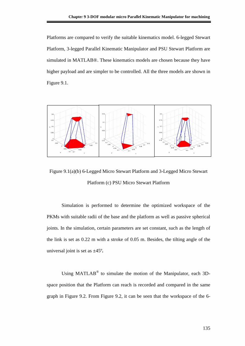
Chapter 9 3-DOF modular micro Parallel Kinematic Manipulator for machining
135
Platforms are compared to verify the suitable kinematics model. 6-legged Stewart
Platform, 3-legged Parallel Kinematic Manipulator and PSU Stewart Platform are
simulated in MATLAB®. These kinematics models are chosen because they have
higher payload and are simpler to be controlled. All the three models are shown in
Figure 9.1.
Figure 9.1(a)(b) 6-Legged Micro Stewart Platform and 3-Legged Micro Stewart
Platform (c) PSU Micro Stewart Platform
Simulation is performed to determine the optimized workspace of the
PKMs with suitable radii of the base and the platform as well as passive spherical
joints. In the simulation, certain parameters are set constant, such as the length of
the link is set as 0.22 m with a stroke of 0.05 m. Besides, the tilting angle of the
universal joint is set as ±45º.
Using MATLAB® to simulate the motion of the Manipulator, each 3D-
space position that the Platform can reach is recorded and compared in the same
graph in Figure 9.2. From Figure 9.2, it can be seen that the workspace of the 6-
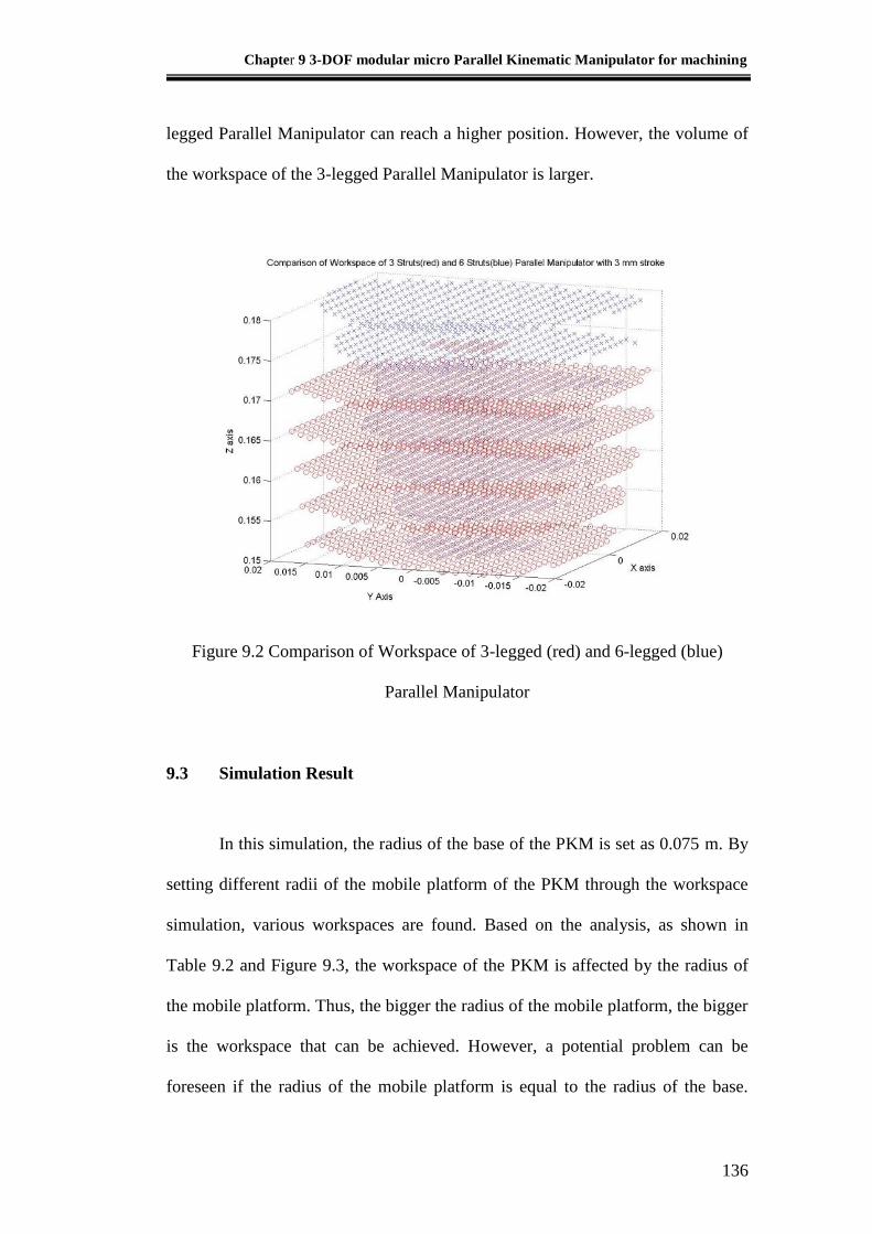
Chapter 9 3-DOF modular micro Parallel Kinematic Manipulator for machining
136
legged Parallel Manipulator can reach a higher position. However, the volume of
the workspace of the 3-legged Parallel Manipulator is larger.
Figure 9.2 Comparison of Workspace of 3-legged (red) and 6-legged (blue)
Parallel Manipulator
9.3 Simulation Result
In this simulation, the radius of the base of the PKM is set as 0.075 m. By
setting different radii of the mobile platform of the PKM through the workspace
simulation, various workspaces are found. Based on the analysis, as shown in
Table 9.2 and Figure 9.3, the workspace of the PKM is affected by the radius of
the mobile platform. Thus, the bigger the radius of the mobile platform, the bigger
is the workspace that can be achieved. However, a potential problem can be
foreseen if the radius of the mobile platform is equal to the radius of the base.
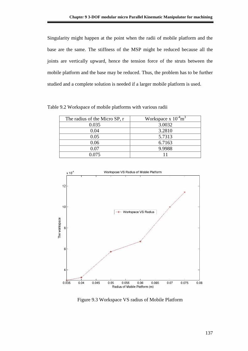
Chapter 9 3-DOF modular micro Parallel Kinematic Manipulator for machining
137
Singularity might happen at the point when the radii of mobile platform and the
base are the same. The stiffness of the MSP might be reduced because all the
joints are vertically upward, hence the tension force of the struts between the
mobile platform and the base may be reduced. Thus, the problem has to be further
studied and a complete solution is needed if a larger mobile platform is used.
Table 9.2 Workspace of mobile platforms with various radii
The radius of the Micro SP, r Workspace x 10-4
m3
0.035 3.0032
0.04 3.2810
0.05 5.7313
0.06 6.7163
0.07 9.9988
0.075 11
Figure 9.3 Workspace VS radius of Mobile Platform
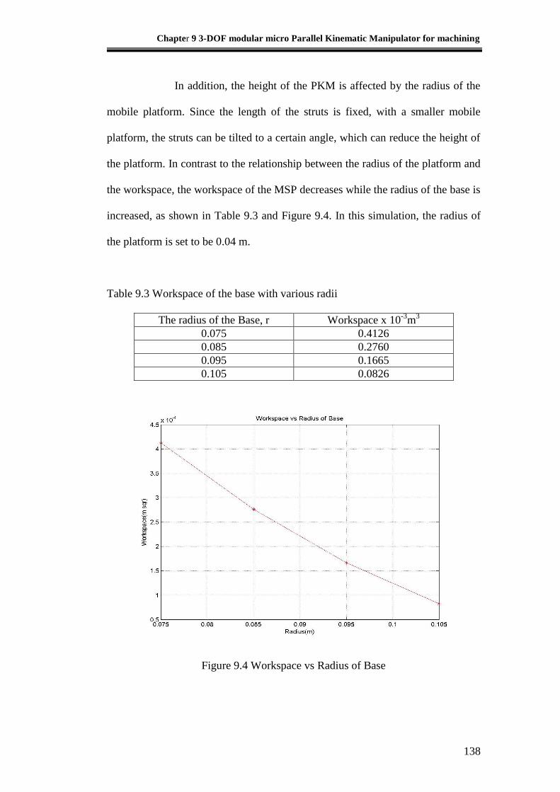
Chapter 9 3-DOF modular micro Parallel Kinematic Manipulator for machining
138
In addition, the height of the PKM is affected by the radius of the
mobile platform. Since the length of the struts is fixed, with a smaller mobile
platform, the struts can be tilted to a certain angle, which can reduce the height of
the platform. In contrast to the relationship between the radius of the platform and
the workspace, the workspace of the MSP decreases while the radius of the base is
increased, as shown in Table 9.3 and Figure 9.4. In this simulation, the radius of
the platform is set to be 0.04 m.
Table 9.3 Workspace of the base with various radii
The radius of the Base, r Workspace x 10-3
m3
0.075 0.4126
0.085 0.2760
0.095 0.1665
0.105 0.0826
Figure 9.4 Workspace vs Radius of Base
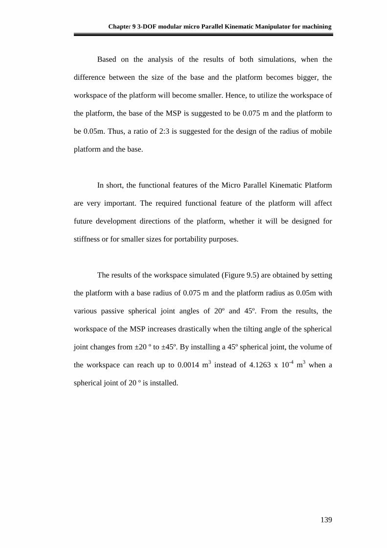
Chapter 9 3-DOF modular micro Parallel Kinematic Manipulator for machining
139
Based on the analysis of the results of both simulations, when the
difference between the size of the base and the platform becomes bigger, the
workspace of the platform will become smaller. Hence, to utilize the workspace of
the platform, the base of the MSP is suggested to be 0.075 m and the platform to
be 0.05m. Thus, a ratio of 2:3 is suggested for the design of the radius of mobile
platform and the base.
In short, the functional features of the Micro Parallel Kinematic Platform
are very important. The required functional feature of the platform will affect
future development directions of the platform, whether it will be designed for
stiffness or for smaller sizes for portability purposes.
The results of the workspace simulated (Figure 9.5) are obtained by setting
the platform with a base radius of 0.075 m and the platform radius as 0.05m with
various passive spherical joint angles of 20º and 45º. From the results, the
workspace of the MSP increases drastically when the tilting angle of the spherical
joint changes from ±20 º to ±45º. By installing a 45º spherical joint, the volume of
the workspace can reach up to 0.0014 m3 instead of 4.1263 x 10
-4 m
3 when a
spherical joint of 20 º is installed.
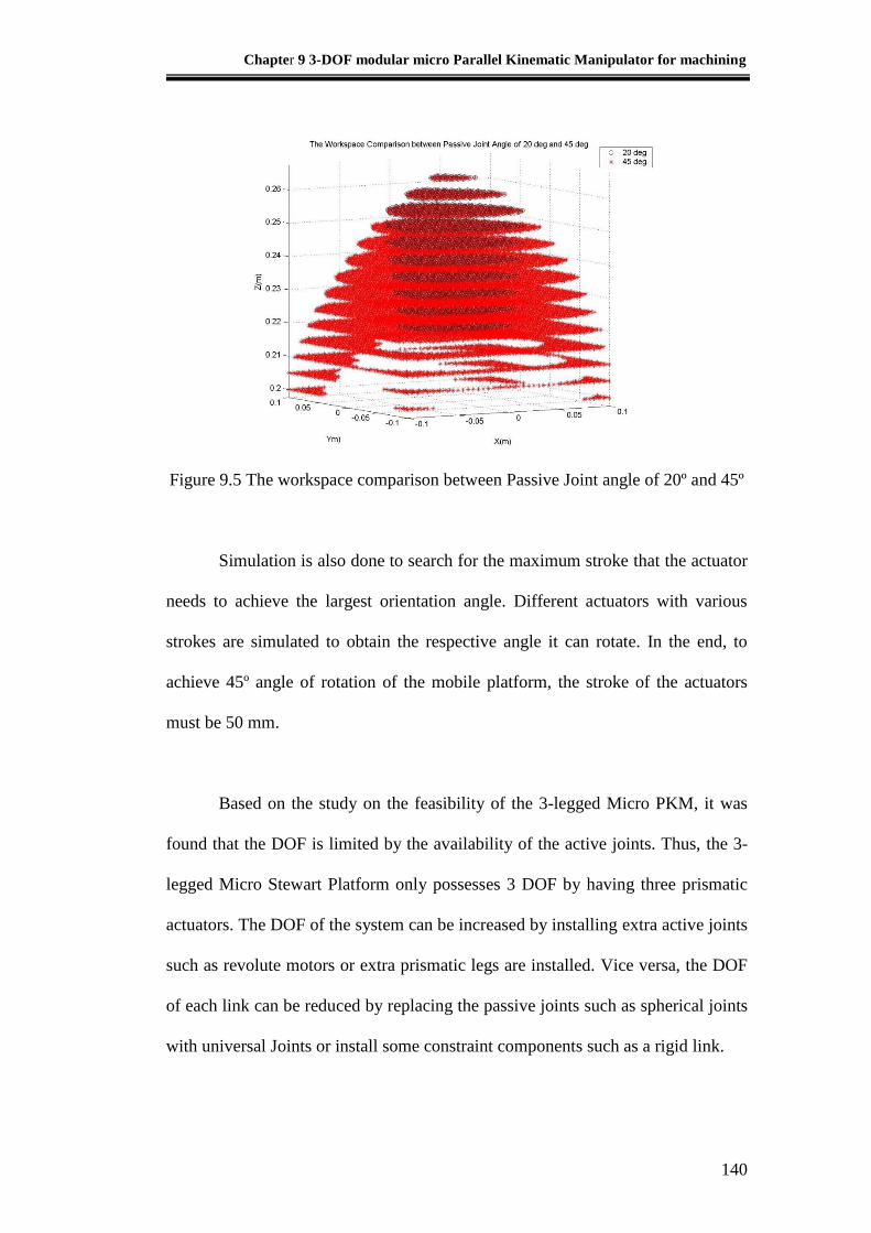
Chapter 9 3-DOF modular micro Parallel Kinematic Manipulator for machining
140
Figure 9.5 The workspace comparison between Passive Joint angle of 20º and 45º
Simulation is also done to search for the maximum stroke that the actuator
needs to achieve the largest orientation angle. Different actuators with various
strokes are simulated to obtain the respective angle it can rotate. In the end, to
achieve 45º angle of rotation of the mobile platform, the stroke of the actuators
must be 50 mm.
Based on the study on the feasibility of the 3-legged Micro PKM, it was
found that the DOF is limited by the availability of the active joints. Thus, the 3-
legged Micro Stewart Platform only possesses 3 DOF by having three prismatic
actuators. The DOF of the system can be increased by installing extra active joints
such as revolute motors or extra prismatic legs are installed. Vice versa, the DOF
of each link can be reduced by replacing the passive joints such as spherical joints
with universal Joints or install some constraint components such as a rigid link.
Chapter 9 3-DOF modular micro Parallel Kinematic Manipulator for machining
141
A 3-DOF Parallel Kinematic Manipulator can be manipulated either purely
in translational or rotational movement. The hybrid of both motions is feasible but
the complexity will be increased. Another method was suggested in [Sameer,
2003], a cooperating hybrid kinematics machine can be constructed by installing a
3-legged orientation mechanism parallel manipulator and a 3-legged translational
mechanism parallel manipulator, a 6-DOF Parallel Kinematic Manipulator system
can be achieved.
In short, based on the result of simulation, a 3-DOF Micro Parallel
Kinematic Manipulator will be constructed with the installation of a 50 mm stroke
actuator and 125 mm diameter platform and 250 mm diameter base to achieve the
requirements of the workspace and functions of the platform.
9.4 Selection of Actuator and Joints
Based on all the previous studies of the Parallel Platform, a M-235.5DG
actuator from PI company is chosen. It has higher loads of 120 N and 100 N of
lateral force; theoretically the three legs can hold literally up to 360 N of load
vertically. It can also achieve micron accuracy in linear motion.
To further increase the degree of orientation mechanism as suggested in
literature study, a Hephaist Spherical Joint from Hephaist Seiko Co. is selected as
shown in Figure 9.6. A Hephaist Spherical Joint is unlike other available spherical
joints in the market. It has a working angle of 40º and can take higher torque.
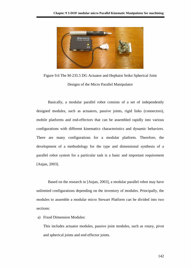
Chapter 9 3-DOF modular micro Parallel Kinematic Manipulator for machining
142
Figure 9.6 The M-235.5 DG Actuator and Hephaist Seiko Spherical Joint
Designs of the Micro Parallel Manipulator
Basically, a modular parallel robot consists of a set of independently
designed modules, such as actuators, passive joints, rigid links (connectors),
mobile platforms and end-effectors that can be assembled rapidly into various
configurations with different kinematics characteristics and dynamic behaviors.
There are many configurations for a modular platform. Therefore, the
development of a methodology for the type and dimensional synthesis of a
parallel robot system for a particular task is a basic and important requirement
[Anjan, 2003].
Based on the research in [Anjan, 2003], a modular parallel robot may have
unlimited configurations depending on the inventory of modules. Principally, the
modules to assemble a modular micro Stewart Platform can be divided into two
sections:
a) Fixed Dimension Modules:
This includes actuator modules, passive joint modules, such as rotary, pivot
and spherical joints and end-effector joints.
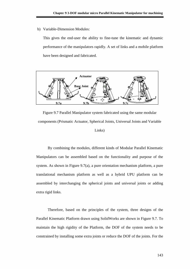
Chapter 9 3-DOF modular micro Parallel Kinematic Manipulator for machining
143
b) Variable-Dimension Modules:
This gives the end-user the ability to fine-tune the kinematic and dynamic
performance of the manipulators rapidly. A set of links and a mobile platform
have been designed and fabricated.
Figure 9.7 Parallel Manipulator system fabricated using the same modular
components (Prismatic Actuator, Spherical Joints, Universal Joints and Variable
Links)
By combining the modules, different kinds of Modular Parallel Kinematic
Manipulators can be assembled based on the functionality and purpose of the
system. As shown in Figure 9.7(a), a pure orientation mechanism platform, a pure
translational mechanism platform as well as a hybrid UPU platform can be
assembled by interchanging the spherical joints and universal joints or adding
extra rigid links.
Therefore, based on the principles of the system, three designs of the
Parallel Kinematic Platform drawn using SolidWorks are shown in Figure 9.7. To
maintain the high rigidity of the Platform, the DOF of the system needs to be
constrained by installing some extra joints or reduce the DOF of the joints. For the
9.7c
Actuator
Base Joint
9.7a 9.7b
Chapter 9 3-DOF modular micro Parallel Kinematic Manipulator for machining
144
4-legged orientation mechanism platform as shown in Figure 9.7(a), a rigid leg
with a spherical joint is installed in the middle of the platform, in order that the
motion of the KPM is limited to angle rotation; thus it can perform pure
orientation movement. Another design of 3 UPU System is shown in Figure 9.7(b),
the spherical joint of the MSP is replaced by Universal Joints. Hence, the platform
system is limited to translational movement by properly orienting the axes of
universal joints. Besides, another 3-DOF Parallel Kinematic Manipulator is set up
as shown in Figure 9.7(c). It is a hybrid 3-DOF platform which consists of
translation movement along Z-axis and orientation around X- and Y-axes.
However, due to the length of the actuator which is 218 mm for 50 mm stroke, it
is quite hard to assemble the whole system inclusive of the joints in the 150 mm x
150 mm x150 mm dimensions. The minimum height that can be achieved with
this system is 250 mm as shown in Figure 9.7. As shown in Figure 9.7(a), by
installing the actuator parallel to the base joint instead of the usual way of
installing the actuator on top of the base joint, the height of the platform can be
reduced to 250 mm. However, the kinematics calculation of the stroke of the
actuator will be more complicated since the actuator is not in-line with the base
joint and spherical joint. A new method of calculation will be shown in the next
section.
Nevertheless, there are certain advantages of installing a 3-DOF micro
parallel platform. The post-processing will be less complex and the stiffness of the
systems can be increased. Furthermore, the modular design concept can be
introduced to the 3-DOF platform. By fabricating interchangeable parts for the
Chapter 9 3-DOF modular micro Parallel Kinematic Manipulator for machining
145
system, the 3-DOF Parallel Kinematic Manipulator can be modified from a
translational platform to a rotational platform. In future, extra legs or active joints
can be bought to increase the DOF of the Micro Parallel Kinematic Manipulator.
A few configurations of the 3 DOF of Stewart Platform were assembled in
the lab as shown in Figure 9.8, such as a pure translational Parallel Kinematic
Manipulator and a pure orientation movement Parallel Kinematic Manipulator.
Translational singularities were detected in the calibration of the pure
translational MSP while it is in the static form. It is verified that in the static
position, extra DOFs are introduced. It is because some geometry conditions are
not met, such as all the revolute pair axes at the leg endings do not converge
towards a single point and every leg has two intermediate resolute pair axes which
are not parallel to one another and are perpendicular to the straight line through
the universal joint center [Gregorio, 2001]. Hence, a careful assembly of the
modular unit of the 3-UPU platform with certain geometry condition is needed to
attain controllable pure translational motion.
Calibrations and various tests were performed on the modular configured.
For the Orientation-Movement Parallel Kinematics Platform, the platform is able
to perform 3-DOF rotational movements in roll, pitch and yaw angles. As all the
links are installed with 2-DOF universal joints, prismatic links and 3-DOF
spherical joints, by installing a fixed link in the middle with a spherical joint, the
motion of the platform will be limited to purely orientation movement around a

Chapter 9 3-DOF modular micro Parallel Kinematic Manipulator for machining
146
Outer part of
the Universal
Joints
Inner part of
the Universal
joints
fixed point. The major disadvantage of this type of configuration is that the
platform cannot perform Z axis movement which is a crucial requirement for
micro machining. The over constrained design of the platform by installing a fixed
middle link will cause the high risk of damaging the platform if it is manipulated
out of the defined workspace.
(a)
(b)
Figure 9.8 (a) Pure Translational Platform, (b) Pure Rotational Platform
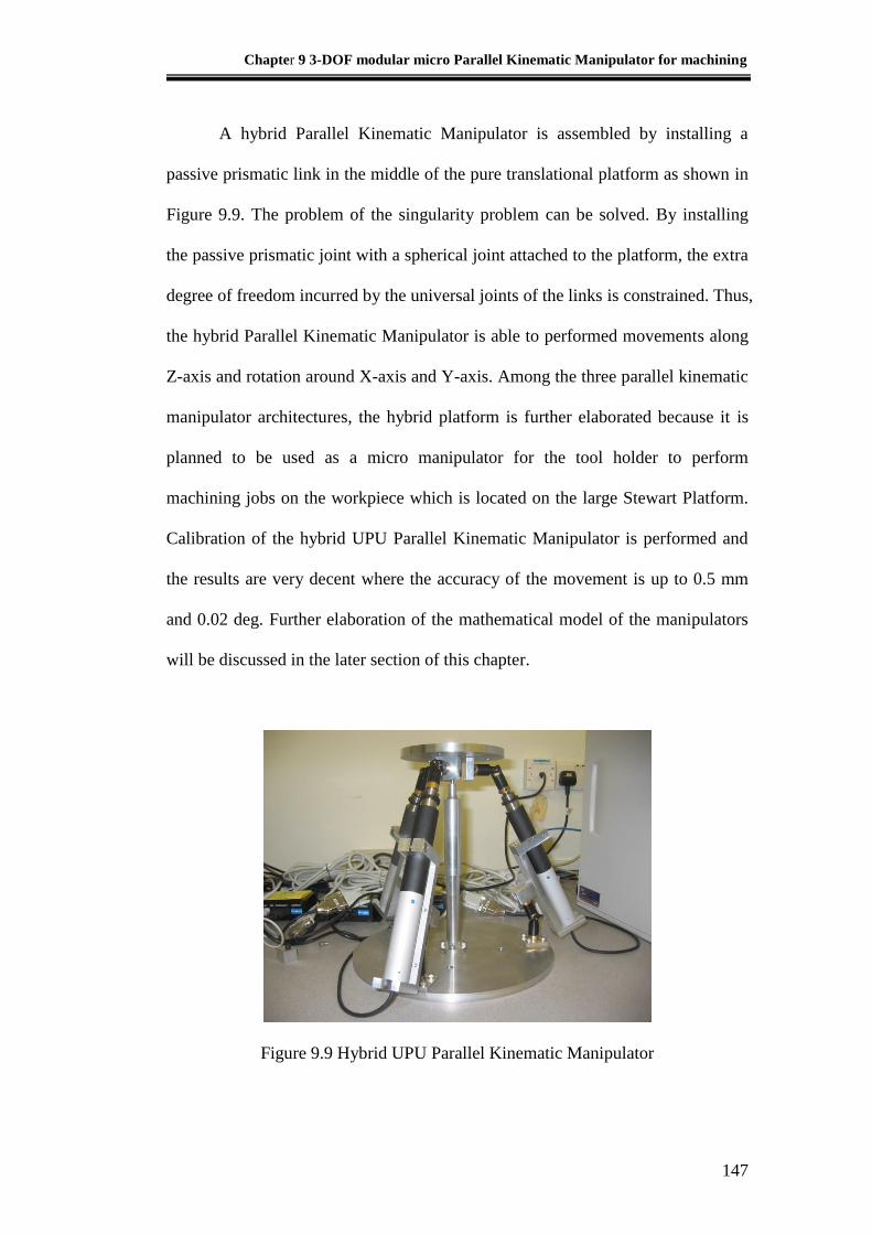
Chapter 9 3-DOF modular micro Parallel Kinematic Manipulator for machining
147
A hybrid Parallel Kinematic Manipulator is assembled by installing a
passive prismatic link in the middle of the pure translational platform as shown in
Figure 9.9. The problem of the singularity problem can be solved. By installing
the passive prismatic joint with a spherical joint attached to the platform, the extra
degree of freedom incurred by the universal joints of the links is constrained. Thus,
the hybrid Parallel Kinematic Manipulator is able to performed movements along
Z-axis and rotation around X-axis and Y-axis. Among the three parallel kinematic
manipulator architectures, the hybrid platform is further elaborated because it is
planned to be used as a micro manipulator for the tool holder to perform
machining jobs on the workpiece which is located on the large Stewart Platform.
Calibration of the hybrid UPU Parallel Kinematic Manipulator is performed and
the results are very decent where the accuracy of the movement is up to 0.5 mm
and 0.02 deg. Further elaboration of the mathematical model of the manipulators
will be discussed in the later section of this chapter.
Figure 9.9 Hybrid UPU Parallel Kinematic Manipulator
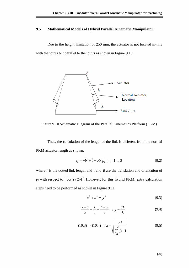
Chapter 9 3-DOF modular micro Parallel Kinematic Manipulator for machining
148
9.5 Mathematical Models of Hybrid Parallel Kinematic Manipulator
Due to the height limitation of 250 mm, the actuator is not located in-line
with the joints but parallel to the joints as shown in Figure 9.10.
Figure 9.10 Schematic Diagram of the Parallel Kinematics Platform (PKM)
Thus, the calculation of the length of the link is different from the normal
PKM actuator length as shown:
iii pRtbl
, i = 1 ... 3 (9.2)
where li is the dotted link length and t
and R are the translation and orientation of
pi with respect to [ XP YP ZP]T. However, for this hybrid PKM, extra calculation
steps need to be performed as shown in Figure 9.11.
222 yax (9.3)
k
xLy
y
yL
a
z
x
xk
(9.4)
1)(
)4.10()3.10(
2
2
2
k
L
ax (9.5)
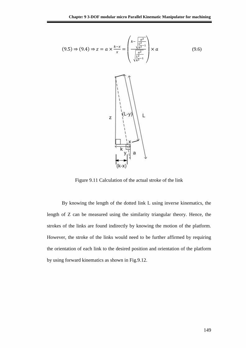
Chapter 9 3-DOF modular micro Parallel Kinematic Manipulator for machining
149
⇒ ⇒
(
√
√
)
(9.6)
Figure 9.11 Calculation of the actual stroke of the link
By knowing the length of the dotted link L using inverse kinematics, the
length of Z can be measured using the similarity triangular theory. Hence, the
strokes of the links are found indirectly by knowing the motion of the platform.
However, the stroke of the links would need to be further affirmed by requiring
the orientation of each link to the desired position and orientation of the platform
by using forward kinematics as shown in Fig.9.12.
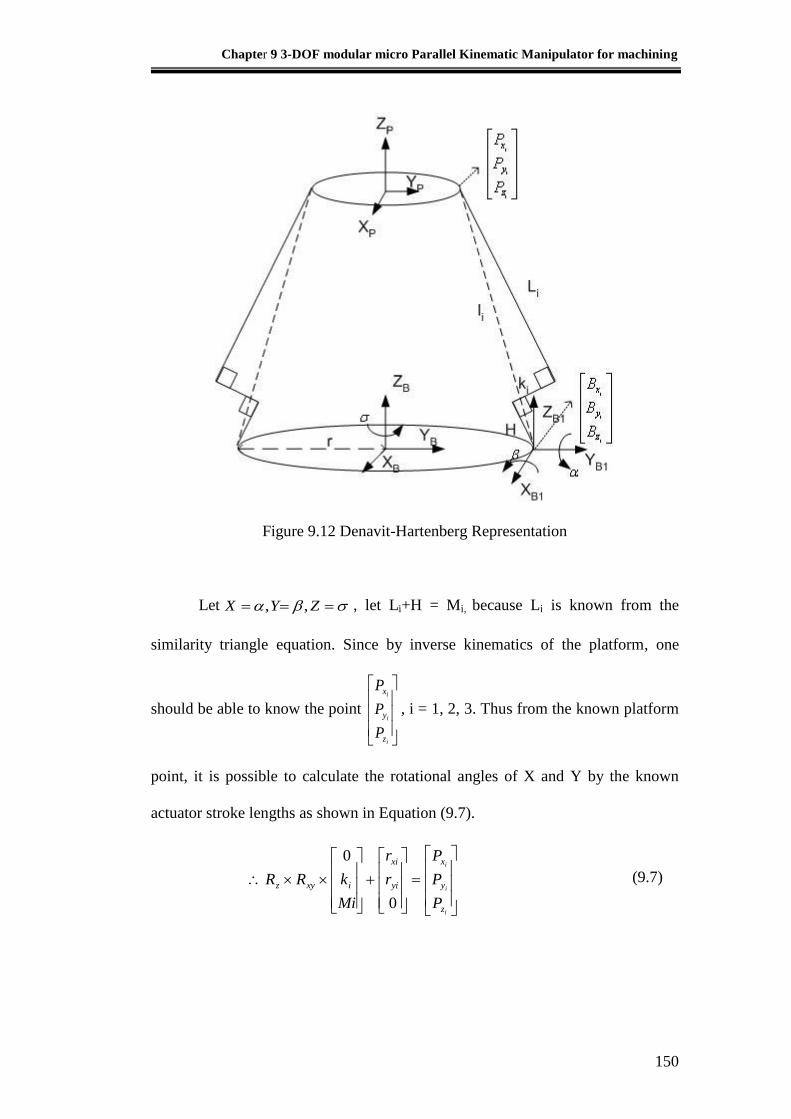
Chapter 9 3-DOF modular micro Parallel Kinematic Manipulator for machining
150
Figure 9.12 Denavit-Hartenberg Representation
Let ZYX ,, , let Li+H = Mi, because Li is known from the
similarity triangle equation. Since by inverse kinematics of the platform, one
should be able to know the point
i
i
i
z
y
x
P
P
P
, i = 1, 2, 3. Thus from the known platform
point, it is possible to calculate the rotational angles of X and Y by the known
actuator stroke lengths as shown in Equation (9.7).
i
i
i
z
y
x
yi
xi
ixyz
P
P
P
r
r
Mi
kRR
0
0
(9.7)
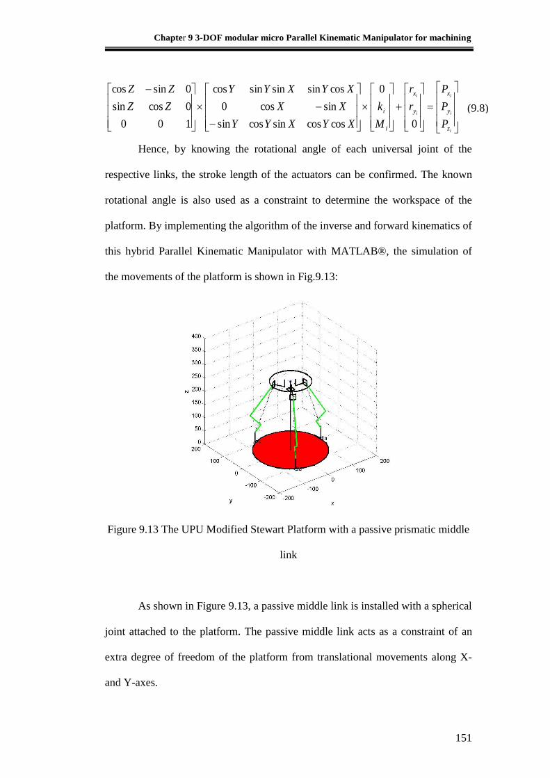
Chapter 9 3-DOF modular micro Parallel Kinematic Manipulator for machining
151
i
i
i
i
i
z
y
x
y
x
i
i
P
P
P
r
r
M
k
XYXYY
XX
XYXYY
ZZ
ZZ
0
0
coscossincossin
sincos0
cossinsinsincos
100
0cossin
0sincos
Hence, by knowing the rotational angle of each universal joint of the
respective links, the stroke length of the actuators can be confirmed. The known
rotational angle is also used as a constraint to determine the workspace of the
platform. By implementing the algorithm of the inverse and forward kinematics of
this hybrid Parallel Kinematic Manipulator with MATLAB®, the simulation of
the movements of the platform is shown in Fig.9.13:
Figure 9.13 The UPU Modified Stewart Platform with a passive prismatic middle
link
As shown in Figure 9.13, a passive middle link is installed with a spherical
joint attached to the platform. The passive middle link acts as a constraint of an
extra degree of freedom of the platform from translational movements along X-
and Y-axes.
(9.8)
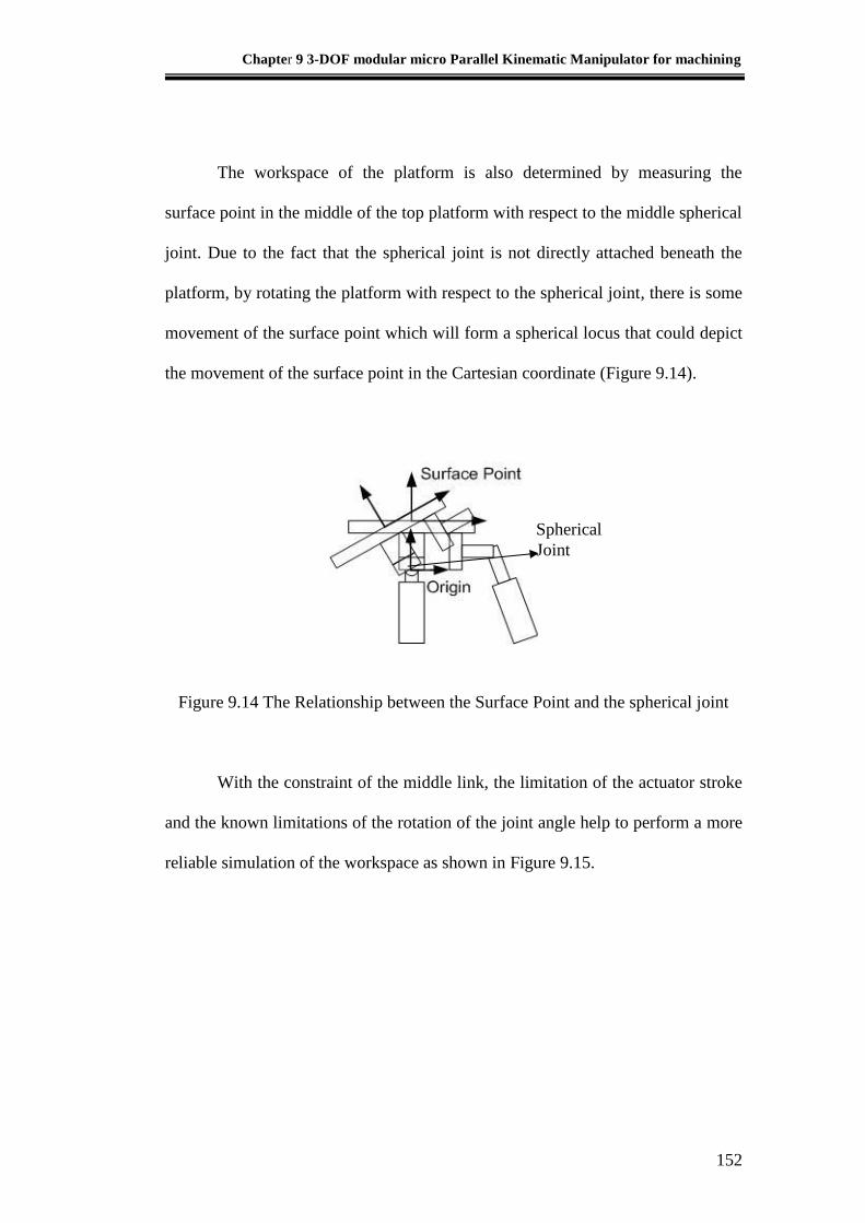
Chapter 9 3-DOF modular micro Parallel Kinematic Manipulator for machining
152
The workspace of the platform is also determined by measuring the
surface point in the middle of the top platform with respect to the middle spherical
joint. Due to the fact that the spherical joint is not directly attached beneath the
platform, by rotating the platform with respect to the spherical joint, there is some
movement of the surface point which will form a spherical locus that could depict
the movement of the surface point in the Cartesian coordinate (Figure 9.14).
Figure 9.14 The Relationship between the Surface Point and the spherical joint
With the constraint of the middle link, the limitation of the actuator stroke
and the known limitations of the rotation of the joint angle help to perform a more
reliable simulation of the workspace as shown in Figure 9.15.
Spherical
Joint
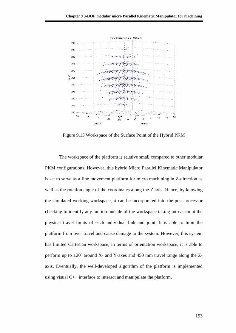
Chapter 9 3-DOF modular micro Parallel Kinematic Manipulator for machining
153
Figure 9.15 Workspace of the Surface Point of the Hybrid PKM
The workspace of the platform is relative small compared to other modular
PKM configurations. However, this hybrid Micro Parallel Kinematic Manipulator
is set to serve as a fine movement platform for micro machining in Z-direction as
well as the rotation angle of the coordinates along the Z axis. Hence, by knowing
the simulated working workspace, it can be incorporated into the post-processor
checking to identify any motion outside of the workspace taking into account the
physical travel limits of each individual link and joint. It is able to limit the
platform from over travel and cause damage to the system. However, this system
has limited Cartesian workspace; in terms of orientation workspace, it is able to
perform up to ±20º around X- and Y-axes and 450 mm travel range along the Z-
axis. Eventually, the well-developed algorithm of the platform is implemented
using visual C++ interface to interact and manipulate the platform.
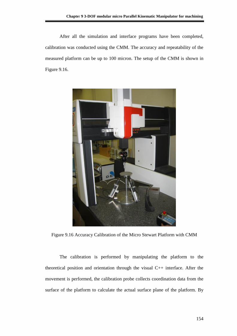
Chapter 9 3-DOF modular micro Parallel Kinematic Manipulator for machining
154
After all the simulation and interface programs have been completed,
calibration was conducted using the CMM. The accuracy and repeatability of the
measured platform can be up to 100 micron. The setup of the CMM is shown in
Figure 9.16.
Figure 9.16 Accuracy Calibration of the Micro Stewart Platform with CMM
The calibration is performed by manipulating the platform to the
theoretical position and orientation through the visual C++ interface. After the
movement is performed, the calibration probe collects coordination data from the
surface of the platform to calculate the actual surface plane of the platform. By
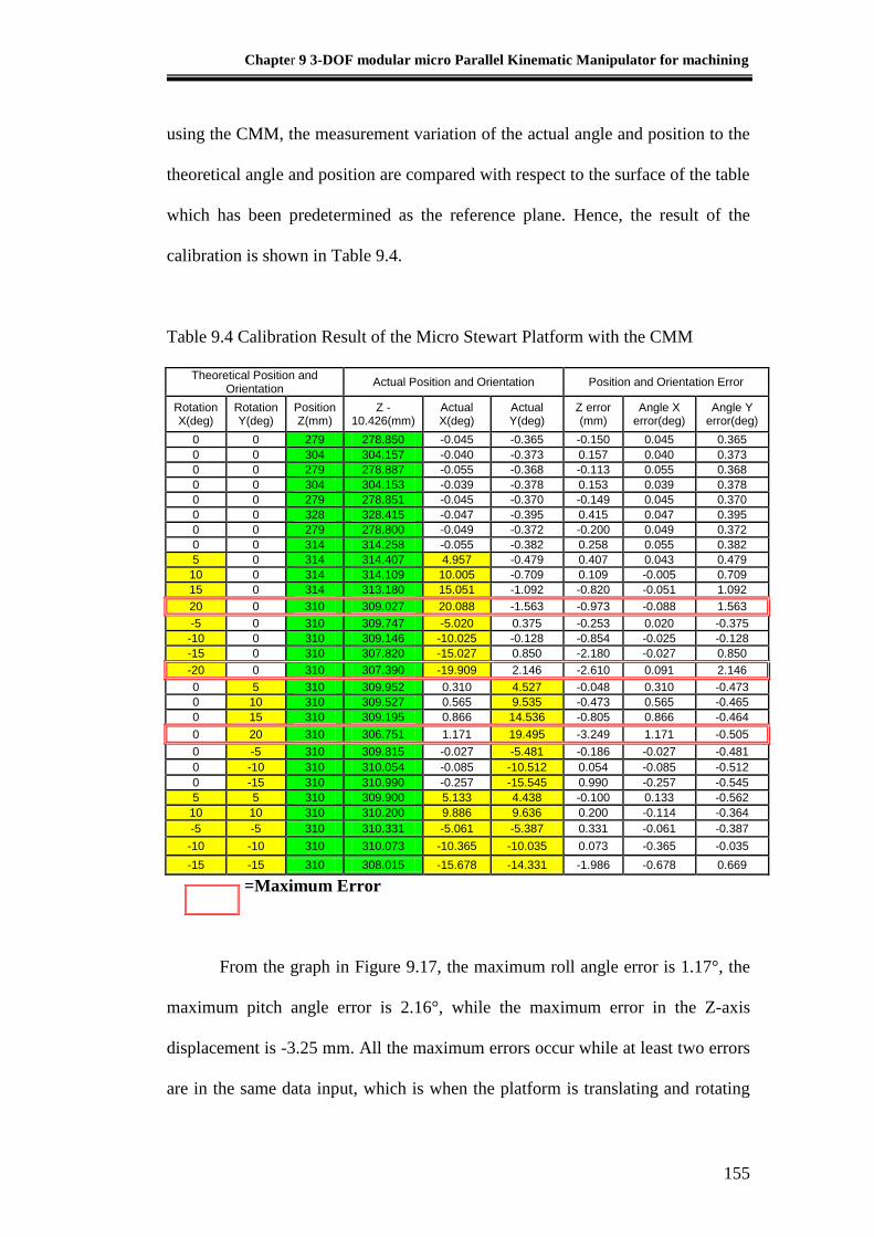
Chapter 9 3-DOF modular micro Parallel Kinematic Manipulator for machining
155
using the CMM, the measurement variation of the actual angle and position to the
theoretical angle and position are compared with respect to the surface of the table
which has been predetermined as the reference plane. Hence, the result of the
calibration is shown in Table 9.4.
Table 9.4 Calibration Result of the Micro Stewart Platform with the CMM
Theoretical Position and Orientation
Actual Position and Orientation Position and Orientation Error
Rotation X(deg)
Rotation Y(deg)
Position Z(mm)
Z -10.426(mm)
Actual X(deg)
Actual Y(deg)
Z error (mm)
Angle X error(deg)
Angle Y error(deg)
0 0 279 278.850 -0.045 -0.365 -0.150 0.045 0.365
0 0 304 304.157 -0.040 -0.373 0.157 0.040 0.373
0 0 279 278.887 -0.055 -0.368 -0.113 0.055 0.368
0 0 304 304.153 -0.039 -0.378 0.153 0.039 0.378
0 0 279 278.851 -0.045 -0.370 -0.149 0.045 0.370
0 0 328 328.415 -0.047 -0.395 0.415 0.047 0.395
0 0 279 278.800 -0.049 -0.372 -0.200 0.049 0.372
0 0 314 314.258 -0.055 -0.382 0.258 0.055 0.382
5 0 314 314.407 4.957 -0.479 0.407 0.043 0.479
10 0 314 314.109 10.005 -0.709 0.109 -0.005 0.709
15 0 314 313.180 15.051 -1.092 -0.820 -0.051 1.092
20 0 310 309.027 20.088 -1.563 -0.973 -0.088 1.563
-5 0 310 309.747 -5.020 0.375 -0.253 0.020 -0.375
-10 0 310 309.146 -10.025 -0.128 -0.854 -0.025 -0.128
-15 0 310 307.820 -15.027 0.850 -2.180 -0.027 0.850
-20 0 310 307.390 -19.909 2.146 -2.610 0.091 2.146
0 5 310 309.952 0.310 4.527 -0.048 0.310 -0.473
0 10 310 309.527 0.565 9.535 -0.473 0.565 -0.465
0 15 310 309.195 0.866 14.536 -0.805 0.866 -0.464
0 20 310 306.751 1.171 19.495 -3.249 1.171 -0.505
0 -5 310 309.815 -0.027 -5.481 -0.186 -0.027 -0.481
0 -10 310 310.054 -0.085 -10.512 0.054 -0.085 -0.512
0 -15 310 310.990 -0.257 -15.545 0.990 -0.257 -0.545
5 5 310 309.900 5.133 4.438 -0.100 0.133 -0.562
10 10 310 310.200 9.886 9.636 0.200 -0.114 -0.364
-5 -5 310 310.331 -5.061 -5.387 0.331 -0.061 -0.387
-10 -10 310 310.073 -10.365 -10.035 0.073 -0.365 -0.035
-15 -15 310 308.015 -15.678 -14.331 -1.986 -0.678 0.669
=Maximum Error
From the graph in Figure 9.17, the maximum roll angle error is 1.17°, the
maximum pitch angle error is 2.16°, while the maximum error in the Z-axis
displacement is -3.25 mm. All the maximum errors occur while at least two errors
are in the same data input, which is when the platform is translating and rotating
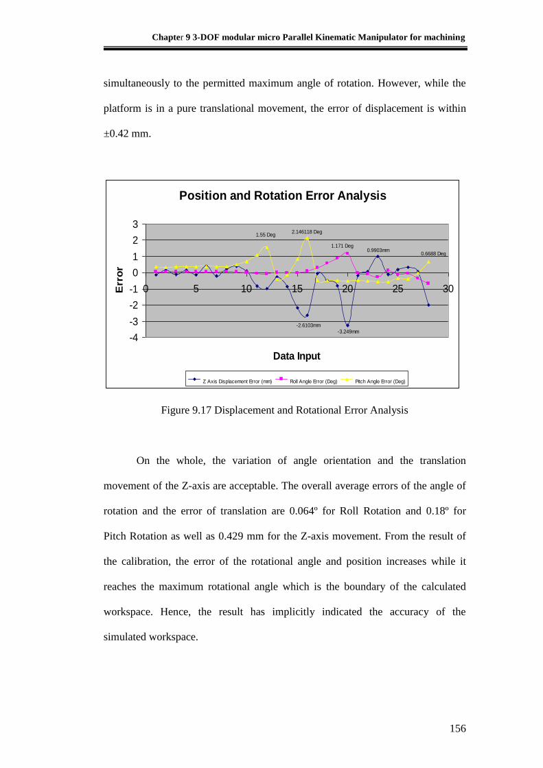
Chapter 9 3-DOF modular micro Parallel Kinematic Manipulator for machining
156
simultaneously to the permitted maximum angle of rotation. However, while the
platform is in a pure translational movement, the error of displacement is within
±0.42 mm.
Figure 9.17 Displacement and Rotational Error Analysis
On the whole, the variation of angle orientation and the translation
movement of the Z-axis are acceptable. The overall average errors of the angle of
rotation and the error of translation are 0.064º for Roll Rotation and 0.18º for
Pitch Rotation as well as 0.429 mm for the Z-axis movement. From the result of
the calibration, the error of the rotational angle and position increases while it
reaches the maximum rotational angle which is the boundary of the calculated
workspace. Hence, the result has implicitly indicated the accuracy of the
simulated workspace.
Position and Rotation Error Analysis
-3.249mm
-2.6103mm
0.9903mm1.171 Deg
0.6688 Deg
2.146118 Deg1.55 Deg
-4
-3
-2
-1
0
1
2
3
0 5 10 15 20 25 30
Data Input
Err
or
Z Axis Displacement Error (mm) Roll Angle Error (Deg) Pitch Angle Error (Deg)
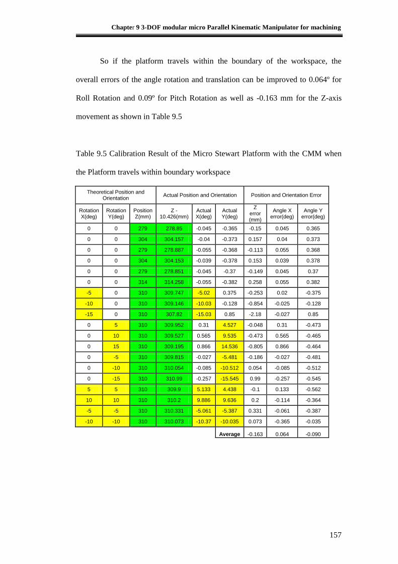
Chapter 9 3-DOF modular micro Parallel Kinematic Manipulator for machining
157
So if the platform travels within the boundary of the workspace, the
overall errors of the angle rotation and translation can be improved to 0.064º for
Roll Rotation and 0.09º for Pitch Rotation as well as -0.163 mm for the Z-axis
movement as shown in Table 9.5
Table 9.5 Calibration Result of the Micro Stewart Platform with the CMM when
the Platform travels within boundary workspace
Theoretical Position and Orientation
Actual Position and Orientation Position and Orientation Error
Rotation X(deg)
Rotation Y(deg)
Position Z(mm)
Z -10.426(mm)
Actual X(deg)
Actual Y(deg)
Z error (mm)
Angle X error(deg)
Angle Y error(deg)
0 0 279 278.85 -0.045 -0.365 -0.15 0.045 0.365
0 0 304 304.157 -0.04 -0.373 0.157 0.04 0.373
0 0 279 278.887 -0.055 -0.368 -0.113 0.055 0.368
0 0 304 304.153 -0.039 -0.378 0.153 0.039 0.378
0 0 279 278.851 -0.045 -0.37 -0.149 0.045 0.37
0 0 314 314.258 -0.055 -0.382 0.258 0.055 0.382
-5 0 310 309.747 -5.02 0.375 -0.253 0.02 -0.375
-10 0 310 309.146 -10.03 -0.128 -0.854 -0.025 -0.128
-15 0 310 307.82 -15.03 0.85 -2.18 -0.027 0.85
0 5 310 309.952 0.31 4.527 -0.048 0.31 -0.473
0 10 310 309.527 0.565 9.535 -0.473 0.565 -0.465
0 15 310 309.195 0.866 14.536 -0.805 0.866 -0.464
0 -5 310 309.815 -0.027 -5.481 -0.186 -0.027 -0.481
0 -10 310 310.054 -0.085 -10.512 0.054 -0.085 -0.512
0 -15 310 310.99 -0.257 -15.545 0.99 -0.257 -0.545
5 5 310 309.9 5.133 4.438 -0.1 0.133 -0.562
10 10 310 310.2 9.886 9.636 0.2 -0.114 -0.364
-5 -5 310 310.331 -5.061 -5.387 0.331 -0.061 -0.387
-10 -10 310 310.073 -10.37 -10.035 0.073 -0.365 -0.035
Average -0.163 0.064 -0.090
Chapter 9 3-DOF modular micro Parallel Kinematic Manipulator for machining
158
9.6 Summary
This chapter addresses the kinematics analysis of the hybrid parallel
mechanism of a hybrid 3-UPU Parallel Mechanism assembled to obtain
translation along the Z-axis and Orientation movements around X- and Y-axes.
The modular configuration of various kinds of parallel kinematics platforms were
successfully assembled with the same modular unit of the respective actuators and
joints. The Hybrid UPU Micro Parallel Kinematics Platform was further studied
and the accuracy of the movement of the platform was calibrated using the CMM
based on the simulated workspace. The errors are acceptable and are limited
within 0.2 deg and 0.5 mm.
The developed inverse kinematic algorithm of the Parallel Kinematic
Manipulator can be applied generally to the same kind of modular configuration
platform by giving a different constraint setting. The algorithm has been
successfully implemented in the control of the hybrid parallel kinematic platform.
The platform is able to travel to the specific position and orientation smoothly and
accurately after calibration with the CMM. The platform is also integrated into a
3-axis machine center to perform machining as shown in Figure 9.18. A designed
workpiece is milled through the integration system as shown in Figure 9.19
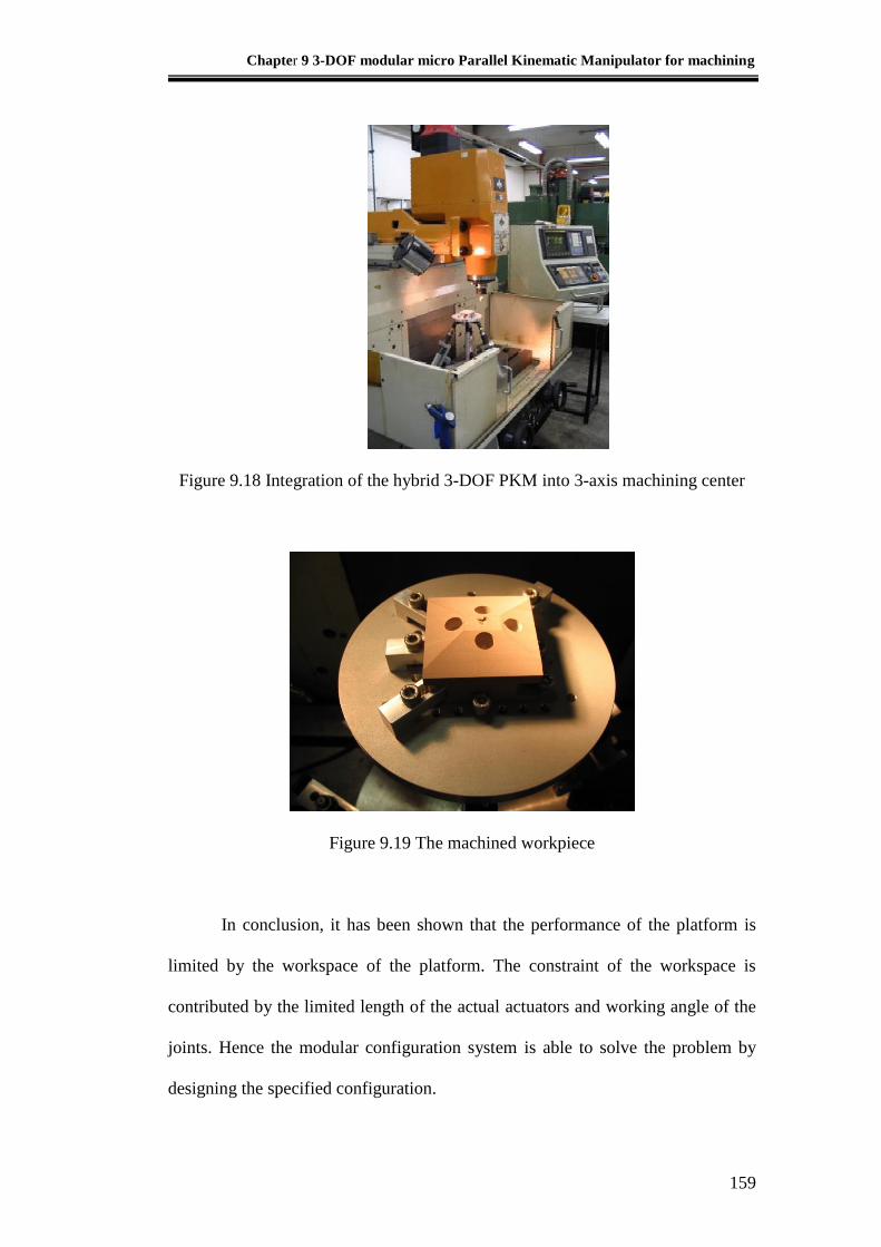
Chapter 9 3-DOF modular micro Parallel Kinematic Manipulator for machining
159
Figure 9.18 Integration of the hybrid 3-DOF PKM into 3-axis machining center
Figure 9.19 The machined workpiece
In conclusion, it has been shown that the performance of the platform is
limited by the workspace of the platform. The constraint of the workspace is
contributed by the limited length of the actual actuators and working angle of the
joints. Hence the modular configuration system is able to solve the problem by
designing the specified configuration.

Chapter 10 Conclusions and Recommendations
160
Chapter 10 Conclusions and Recommendations
10.1 Conclusions
A Gough-Stewart Platform has been fabricated and developed in this
research. Software development was completed on the Stewart Platform for this
study so that users can communicate with the controller of the Stewart Platform
with standard NC codes through building models using commercial CAD/CAM
systems.
In this research, the kinematics of the system was studied. The forward
kinematics problem cannot be solved easily compared to the case of a serial
manipulator. However, the inverse kinematics of the parallel manipulator is found
to have a direct solution. Nevertheless, the forward kinematics can be solved by
using the Newton Raphson numerical method. The developed forward kinematics
can also help develop a proper feedback system for the Stewart Platform. The
installation of the wire sensors helps to predict the final position and orientation of
the end-effector of the mobile platform by knowing the length of the actuators. In
addition, the dynamics of the system was investigated and simulation was done by
using MATLAB® SimMechanics in the study.
The kinematics analysis of the hybrid parallel mechanism was also studied.
A hybrid 3-UPU Parallel Mechanism was assembled to obtain the motion of
translation along the Z-axis and Orientation movement around X- and Y-axes.
Modular configurations of various kinds of parallel kinematics platforms were
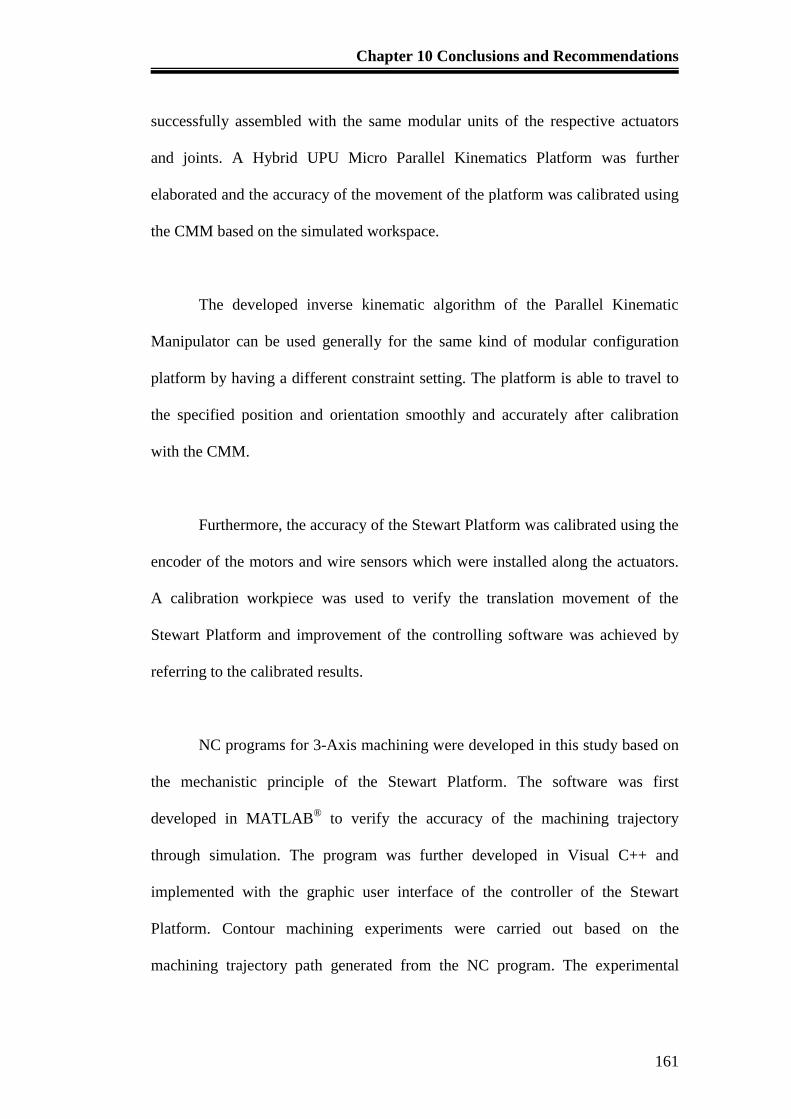
Chapter 10 Conclusions and Recommendations
161
successfully assembled with the same modular units of the respective actuators
and joints. A Hybrid UPU Micro Parallel Kinematics Platform was further
elaborated and the accuracy of the movement of the platform was calibrated using
the CMM based on the simulated workspace.
The developed inverse kinematic algorithm of the Parallel Kinematic
Manipulator can be used generally for the same kind of modular configuration
platform by having a different constraint setting. The platform is able to travel to
the specified position and orientation smoothly and accurately after calibration
with the CMM.
Furthermore, the accuracy of the Stewart Platform was calibrated using the
encoder of the motors and wire sensors which were installed along the actuators.
A calibration workpiece was used to verify the translation movement of the
Stewart Platform and improvement of the controlling software was achieved by
referring to the calibrated results.
NC programs for 3-Axis machining were developed in this study based on
the mechanistic principle of the Stewart Platform. The software was first
developed in MATLAB® to verify the accuracy of the machining trajectory
through simulation. The program was further developed in Visual C++ and
implemented with the graphic user interface of the controller of the Stewart
Platform. Contour machining experiments were carried out based on the
machining trajectory path generated from the NC program. The experimental
Chapter 10 Conclusions and Recommendations
162
results were quite accurate but unevenness of the motion of the platform was
detected during the machining process.
After 3-Axis machining has been successfully implemented with the
control system of the Stewart Platform, 5-axis machining was further developed.
The 5-axis machining trajectory path was developed using MATLAB® by
performing conversion of the local coordinate system of the freeform surface to
the trajectory path based on the machining coordinate system. In addition, the
Stewart Platform is found to have advantages over 5-axis CNC machine in terms
of mechanical design and the simplicity of the inverse kinematics towards
orientation and translation of the end-effector of the mobile platform to achieve 5-
axis motion.
At the completion of the project, all the developed programs and
algorithms were integrated into one single user interface to manipulate the motion
of the Stewart Platform. Thus, users can control the movement of the Stewart
Platform by issuing parameters either in terms of the orientation and position of
the mobile platform or the extracted length of the actuator. The machining process
of the Stewart Platform can also be achieved by using the input of the NC
program. In conclusion, the study of 3D and 5D machining of the Stewart
Platform has been achieved in this research.
Chapter 10 Conclusions and Recommendations
163
10.2 Recommendations for Future Work
Even though the objectives of the project have been achieved, further
study can be carried out to improve the quality of the machining process on the
Stewart Platform. Some future work can be focused on the following aspects.
Workspace
The Parallel Kinematic Manipulator is well known for its workspace
limitation. Hence, to improve the workspace of the Stewart Platform, two methods
are suggested. One method is to replace the existent spherical joints with larger
working angle spherical joints. Another method is the collaboration of two
Stewart Platforms to form a single system to perform the machining task.
However, several challenges would need to be overcome, such as the
synchronization of the motion of the Stewart Platforms to achieve the same
position at the same time. There will also be problems to assure the allocation of
the two Stewart Platforms is within the working workspace concurrently such that
the platforms can have the same stiffness and rigidity.
Accuracy of the Platform
There are some limitations of the accuracy of the platform since the
current Stewart Platform was driven by stepper motors. Hence, a servomotor
system Stewart Platform is currently being developed in the Advanced
Manufacturing Lab. By using a servomotor system, the Stewart Platform can be
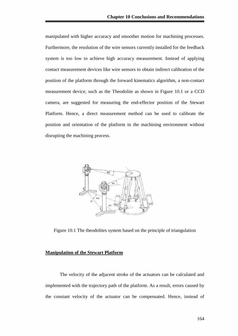
Chapter 10 Conclusions and Recommendations
164
manipulated with higher accuracy and smoother motion for machining processes.
Furthermore, the resolution of the wire sensors currently installed for the feedback
system is too low to achieve high accuracy measurement. Instead of applying
contact measurement devices like wire sensors to obtain indirect calibration of the
position of the platform through the forward kinematics algorithm, a non-contact
measurement device, such as the Theodolite as shown in Figure 10.1 or a CCD
camera, are suggested for measuring the end-effector position of the Stewart
Platform. Hence, a direct measurement method can be used to calibrate the
position and orientation of the platform in the machining environment without
disrupting the machining process.
Figure 10.1 The theodolites system based on the principle of triangulation
Manipulation of the Stewart Platform
The velocity of the adjacent stroke of the actuators can be calculated and
implemented with the trajectory path of the platform. As a result, errors caused by
the constant velocity of the actuator can be compensated. Hence, instead of
Chapter 10 Conclusions and Recommendations
165
controlling the platform to move from point to point, the platform can now be
controlled using the velocity profile. The most popular way to control the Stewart
Platform is using a linear (PID-like) control law at the joint level and a simple
inverse kinematics algorithm on top of the control loop.
In short, better and more reliable calibration experiments must be
developed to further improve the accuracy of motion of the Stewart Platform, so
that it can be optimized for machining tasks. These mentioned issues will be the
challenges for future Stewart Platform research.

References
166
References
1. [Alyushin, 2010] Alyushin, Y.A., and Elenev, S.A., “Mathematical Model of
Stewart Platform Motion”, Journal of Machinery Manufacture and Reliability,
2010, Vol. 39, No 4, pp 305-312
2. [Anjan, 2003] Dash, A.K., Chen, I.M., Yeo, S.H., and Yang, G.L., “Task-
Based Configuration Design for 3-Legged Modular Parallel Robots Using
Simplex Methods” Computational Intelligence in Robotics and Automation,
2003. Proceedings. 2003 IEEE International Symposium, vol.2 998 - 1003
3. [Arai, 1991] Arai, T., Cleary, K., Homma, K., Adachi, H. and Nakamura, T.,
1991, “Development of Parallel Link Manipulator for Underground
Excavation Task,” 1991 International Symposium on Advanced Robot
Technology, pp.541-548.
4. [Asada, 1985] Asada, H., and Cro Granito, J.A., 1985, “Kinematic and
Static Characterization of Wrist Joints and Their Optimal Design” Proceedings
of IEEE International Conference on Robotics and Automation, St. Louis, pp.
91-100.
5. [Badescu, 2002] Badescu, M., Morman, J., and Mavroidis, C., 2002,
“Workspace Optimization of Orientational 3-Legged UPS Parallel Platforms”,
Proceedings of DETC’02 ASME 2002 Design Engineering Technical
Conferences and Computers and Information in Engineering Conference.
6. [Bonev, 1999] Bonev, I.A. and Ryu, J., 1999, “Orientation Workspace
Analysis of 6-DOF Parallel Manipulators”, Proceedings of the 1999 ASME
References
167
Design Engineering Technical Conferences September 12-15, 1999, Las
Vegas, Nevada, USA.
7. [Chan, 2001] Chan, V., 2001, “Singularity Analysis and Redundant Actuation
of Parallel Manipulators” M Eng Thesis, The Ohio State University , pp. 5-50
8. [Charles, 1991] Nguyen, C.C., Zhou, Z.-L., Antrazi, S.S., and Campbell,
C.E., Jr., 1991, “Efficient computation of forward kinematics and Jacobian
matrix of a Stewart platform-based manipulator”, IEEE Proceedings of
Southeast conference '91, 7-10 April 1991, vol.2 , pp 869 - 874
9. [Clavel, 1988] Clavel, R., 1988 “DELTA, A Fast Robot With Parallel
Geometry,” 18th
International Symposium on Industrial Robots, pp. 91 -100,
April.
10. [Craig, 1986] Craig, J.J., 1986, “Introduction To Robotic Mechanics and
Control”, 2nd
Edition, Addison Wesley Publishing Company Inc, pp.278-279
11. [Eric, 1996] Eric, P. and Reymond, C., 1996, “Parallel Robots And
Microbotics”, Volume 6, Robotics and manufacturing: Recent Trends in
Research and Applications edited by M. Jamshid, F. Pin and P. Dauchez,
ASME Press, pp 35.
12. [Fassi, 2000] Fasssi, I. and Weins, G.J., 2000, “Multi Axis Machining : PKMs
and Traditional Machining Centers”, Journal of Manufacturing Processes;
2000; 2,1: ABI/INFORM Global pp.1
13. [Faux, 1979] Faux, I.D. and Pratt, M.J.,1979, “Computational Geometry for
Design and Manufacture, Ellis Horwood
14. [Gregorio, 2001] Gregorio, R.D., 2001, “Statics and Singularity Loci of the 3-
UPU Wrist”, 2001 IEEE/ASME International Conference on Advanced
References
168
Intelligent Mechatronics Proceedings 8-12 July 2001, Como, Italy. Pp 470-
475
15. [Gosselin, 1989] Gosselin, C. and Angeles, J., 1989, “The Optimum
Kinematics Design of a Spherical Three-Degree-Freedom Camera –
Orientation Device,” IEEE Int. Conference on Robotics and Automation, pp.
781-786.
16. [Gough, 1962] Gough V.E. and Whitehall, S.G., 1962, “Universal Tyre Test
Machine,” Proc. 9th
Int’l Tech. Congress, F.I.S.I.T.A, 177 (Institution of
Mechanical Engineers).
17. [Gosselin, 1994] Gosselin, C., and Hamel, J., 1994, “The Agile Eye: Agile
Performance Three-Degree-of Freedom Camera-Orienting Device,” IEEE
International Conference on Robotics and Automation, pp. 781-786.
18. [Hunt, 1983] Hunt, K.H., 1983, “Structural Kinematics of In-Parallel-
Actuated Robot-Arms,” ASME Journal of Mechanisms, Transmissions, and
Automation in Design, Vol. 105, pp. 705-712.
19. [Huynh, 2001] Huynh, P., 2001, “Kinematics Performance Comparison of
Linear Type Parallel Mechanisms Application To The Design And Control of
A Hexaslide”, 5th
International Conference on Mechatronics Technology, June
6-8, 2001, National University of Singapore. pp. 1-8
20. [Jakobovic, 2002] Jakobovic, D. and Jelenkovic, L. 2002, “The Forward and
Inverse Kinematics Problems for Stewart Parallel Mechanisms” Proc. 8th Int.
Scientific Conference on Production Engineering CIM 2002, Brijuni, June 13-
14.
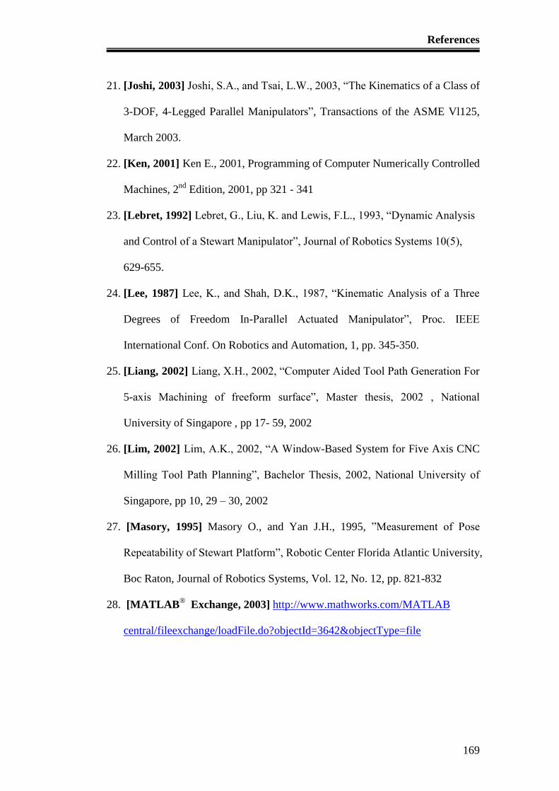
References
169
21. [Joshi, 2003] Joshi, S.A., and Tsai, L.W., 2003, “The Kinematics of a Class of
3-DOF, 4-Legged Parallel Manipulators”, Transactions of the ASME Vl125,
March 2003.
22. [Ken, 2001] Ken E., 2001, Programming of Computer Numerically Controlled
Machines, 2nd
Edition, 2001, pp 321 - 341
23. [Lebret, 1992] Lebret, G., Liu, K. and Lewis, F.L., 1993, “Dynamic Analysis
and Control of a Stewart Manipulator”, Journal of Robotics Systems 10(5),
629-655.
24. [Lee, 1987] Lee, K., and Shah, D.K., 1987, “Kinematic Analysis of a Three
Degrees of Freedom In-Parallel Actuated Manipulator”, Proc. IEEE
International Conf. On Robotics and Automation, 1, pp. 345-350.
25. [Liang, 2002] Liang, X.H., 2002, “Computer Aided Tool Path Generation For
5-axis Machining of freeform surface”, Master thesis, 2002 , National
University of Singapore , pp 17- 59, 2002
26. [Lim, 2002] Lim, A.K., 2002, “A Window-Based System for Five Axis CNC
Milling Tool Path Planning”, Bachelor Thesis, 2002, National University of
Singapore, pp 10, 29 – 30, 2002
27. [Masory, 1995] Masory O., and Yan J.H., 1995, ”Measurement of Pose
Repeatability of Stewart Platform”, Robotic Center Florida Atlantic University,
Boc Raton, Journal of Robotics Systems, Vol. 12, No. 12, pp. 821-832
28. [MATLAB®
Exchange, 2003] http://www.mathworks.com/MATLAB
central/fileexchange/loadFile.do?objectId=3642&objectType=file
References
170
29. [Mckee, 1999] Mckee, G. and Schenker, P., Editors, 1999, sensor Fusion
and Decentralized control in Robotic Systems II, SPIE Proceeding Series, Vol.
3839.
30. [Mortenson, 1985] Mortenson M.E. 1985, Geometric Modeling, John Wiley
31. [Neugebauer, 2000] Neugebauer, R., Wieland, F., and Ihlenfeldt, S., 2000,
“Comparison of parallel structure concepts for five-axis machining”, Journal
of Manufacturing Processes; 2000; 2, 1; ABI/INFORM Global pp 59-66
32. [Neugebauer, 2000] Neugebauer, R., Wieland, F., and Ihlenfeldt, S., 2002,
“Comparison of parallel structure concepts for five-axis Machining”, Journal
of Manufacturing Processes , 1, ABI/INFORM Global pp. 59
33. [Piegl, 1991] Piegl L., 1991 “On NURBS: a survey, IEEE Computer Graphics
and Application”, Jan 1991
34. [Reinholz, 1987] Reinholz, C. and Gokhale D., 1987,”Design and Analysis of
Variable Geometry Truss Robot,” Proc. 9th
Applied Mechanism Conference,
Oklahoma State University.
35. [Shih, 2003] Shih, C.Y., 2003, “An Impedance Control Design and
Simulation of Stewart Platform with Fuzzy Neural Network Compensator”,
Master Thesis, Chung Yuan Christian University, pp 20 – 26
36. [Sternheim, 1987] Sternheim, F., 1987, “Computation of the Direct and
Inverse Kinematics Model of the Delta 4 Parallel Robot,” Robotersysteme, 3,
pp. 199-203.
37. [Stewart, 1965] Stewart, D., 1965, “A Platform with Six Degrees of Freedom,”
Proc. Institute of Mechanical Engr., London, England, Vol. 180, pp.371-386.
References
171
38. [Tlusty, 2000] Tlusty, J., Ziegert, J.C., and Ridgeway, S., 2000, ‘A
Comparison of Stiffness Characteristics of Serial and Parallel Machine Tools’,
Journal of Manufacturing Processes; 2000; 2,1; ABI/INFORM Global , pp 67
– 76
39. [Tsai, 1996] Tsai, L.W., 1996, “Kinematics of a Three-DOF Platform With
Three Extensible Limbs”, Recent Advances in Robot Kinematics, 401-410,
Kluwer Academic Publishers pp.401-402
40. [Tsai, 1996] Tsai, L.W., Walsh, G.C., and Stamper, R.E., 1996, “Kinematics
of a Novel Three DOF Translational Platform”, Proceedings of the 1996 IEEE
International Conference on Robotics and Automation Minneapolis,
Minnesota – April 1996.
41. [Tsai, 1999]Tsai, L.W., 1999, “Robot analysis, “The Mechanics of Serial and
Parallel Manipulators”, John Wiley & Sons, INC, pp169 – 433
42. [Tsai, 2000]Tsai, L.W., 2000, Mechanism Design: Enumeration of Kinematic
Structures According to Function, ISBN 0-8493-0901-8, CRC Press, Boca
Raton, FL.
43. [Tsai, 2002] Tsai, L.W., and Joshi, S., “Kinematic Analysis of 3-DOF
Position Mechanisms for Use in Hybrid Kinematic Machines”, Journal of
Mechanical Design, June 2002, Vol 124, Pp 245-253
44. [Yang, 2003] Yang, G.L., Chen, I.M., Chen, W.H., and Yeo, S.H., 2003,
“Design and Analysis of a 3-RPRS Modular Parallel Manipulator for Rapid
Deployment", Proceedings of the 2003 IEEE/ASME International Conference
on Advanced Intelligent Mechatronics (AIM 2003), pp 1250-1255
Appendix A: NC Code tables
172
Appendices
Appendix A: NC Code tables
Table A1 Address characters [Ken, 2001]
Character Meaning
A Additional rotary axis parallel and around the X-axis
B Additional rotary axis parallel and around the Y-axis
C Additional rotary axis parallel and around the Z-axis
D Tool radius offset number, depth of cut for multiple repetitive cycles
E User macro character, precise designation of thread lead
F Feed rate, precise designation of thread lead
G Preparatory function
H Tool length offset number
I Incremental X-coordinate of circle center or parameter of fixed cycle
J Incremental Y-coordinate of circle center
K Incremental Z-coordinate of circle center or parameter of fixed cycle
L Number of repetition
M Miscellaneous function
N Sequence or block number
O Program number
P Dwell time, program number, and sequence number designation in
subprogram; Sequence number for multiple repetitive cycles
Q Depth of cut, shift of canned cycles; Sequence number for multiple
repetitive cycles
R Point R for canned cycles, as a reference return value; Radius
designation of a cycle arc
S Spindle-speed function
T Tool-function
U Additional linear axis parallel to X-axis
V Additional linear axis parallel to Y-axis
W Additional linear axis parallel to Z-axis
X X-coordinate
Y Y-coordinate
Z Z-coordinate
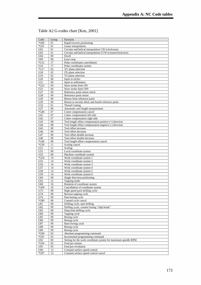
Appendix A: NC Code tables
173
Table A2 G-codes chart [Ken, 2001]
Code Group Function
*G00 01 Rapid traverse positioning
*G01 01 Linear interpolation
G02 01 Circular and helical interpolation CW (clockwise)
G03 01 Circular and helical interpolation CCW (counterclockwise)
G04 00 Dwell
G09 00 Exact stop
*G15 17 Polar coordinates cancellation
G16 17 Polar coordinates system
*G17 02 XY plane selection
G18 02 ZX plane selection
G19 02 YZ plane selection
G20 06 Input in inches
G21 06 Input in millimeters
*G22 04 Store stroke limit ON
G23 04 Store stroke limit OFF
G27 00 Reference point return check
G28 00 Reference point return
G29 00 Return from reference point
G30 00 Return to second, third, and fourth reference point
G33 01 Thread Cutting
G37 00 Automatic tool length measurement
*G40 07 Cutter compensation cancel
G41 07 Cutter compensation left side
G42 07 Cutter compensation right side
G43 08 Tool length offset compensation positive (+) direction
G44 08 Tool length offset compensation negative (-) direction
G45 00 Tool offset increase
G46 00 Tool offset decrease
G47 00 Tool offset double increase
G48 00 Tool offset double decrease
*G49 08 Tool length offset compensation cancel
*G50 11 Scaling cancel
G51 11 Scaling
G52 00 Local coordinate system
G53 00 Machine coordinate system
*G54 14 Work coordinate system 1
G55 14 Work coordinate system 2
G56 14 Work coordinate system 3
G57 14 Work coordinate system 4
G58 14 Work coordinate system 5
G59 14 Work coordinate system 6
G60 00 Single direction positioning
G63 15 Tapping mode
G68 16 Rotation of coordinate system
*G69 16 Cancellation of coordinate system
G73 09 High speed peck drilling cycle
G74 09 Reverse tapping cycle
G76 09 Fine boring cycle
*G80 09 Canned cycle cancel
G81 09 Drilling cycle, spot drilling
G82 09 Drilling cycle, counter boring “chip break”
G83 09 Deep hole drilling cycle
G84 09 Tapping cycle
G85 09 Boring cycle
G86 09 Boring cycle
G87 09 Back boring cycle
G88 09 Boring cycle
G89 09 Boring cycle
*G90 03 Absolute programming command
*G91 03 Incremental programming command
G92 00 Setting for the work coordinate system for maximum spindle RPM
*G94 05 Feed per minute
G95 05 Feed per revolution
G96 13 Constant surface speed control
*G97 13 Constant surface speed control cancel
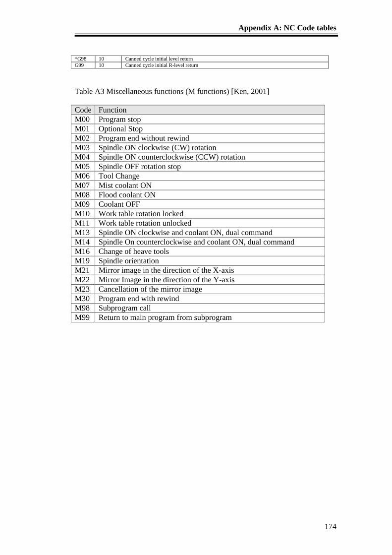
Appendix A: NC Code tables
174
*G98 10 Canned cycle initial level return
G99 10 Canned cycle initial R-level return
Table A3 Miscellaneous functions (M functions) [Ken, 2001]
Code Function
M00 Program stop
M01 Optional Stop
M02 Program end without rewind
M03 Spindle ON clockwise (CW) rotation
M04 Spindle ON counterclockwise (CCW) rotation
M05 Spindle OFF rotation stop
M06 Tool Change
M07 Mist coolant ON
M08 Flood coolant ON
M09 Coolant OFF
M10 Work table rotation locked
M11 Work table rotation unlocked
M13 Spindle ON clockwise and coolant ON, dual command
M14 Spindle On counterclockwise and coolant ON, dual command
M16 Change of heave tools
M19 Spindle orientation
M21 Mirror image in the direction of the X-axis
M22 Mirror Image in the direction of the Y-axis
M23 Cancellation of the mirror image
M30 Program end with rewind
M98 Subprogram call
M99 Return to main program from subprogram
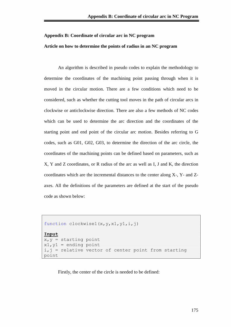
Appendix B: Coordinate of circular arc in NC Program
175
Appendix B: Coordinate of circular arc in NC program
Article on how to determine the points of radius in an NC program
An algorithm is described in pseudo codes to explain the methodology to
determine the coordinates of the machining point passing through when it is
moved in the circular motion. There are a few conditions which need to be
considered, such as whether the cutting tool moves in the path of circular arcs in
clockwise or anticlockwise direction. There are also a few methods of NC codes
which can be used to determine the arc direction and the coordinates of the
starting point and end point of the circular arc motion. Besides referring to G
codes, such as G01, G02, G03, to determine the direction of the arc circle, the
coordinates of the machining points can be defined based on parameters, such as
X, Y and Z coordinates, or R radius of the arc as well as I, J and K, the direction
coordinates which are the incremental distances to the center along X-, Y- and Z-
axes. All the definitions of the parameters are defined at the start of the pseudo
code as shown below:
function clockwise1(x,y,x1,y1,i,j)
Input
x,y = starting point
x1,y1 = ending point
i,j = relative vector of center point from starting
point
Firstly, the center of the circle is needed to be defined:
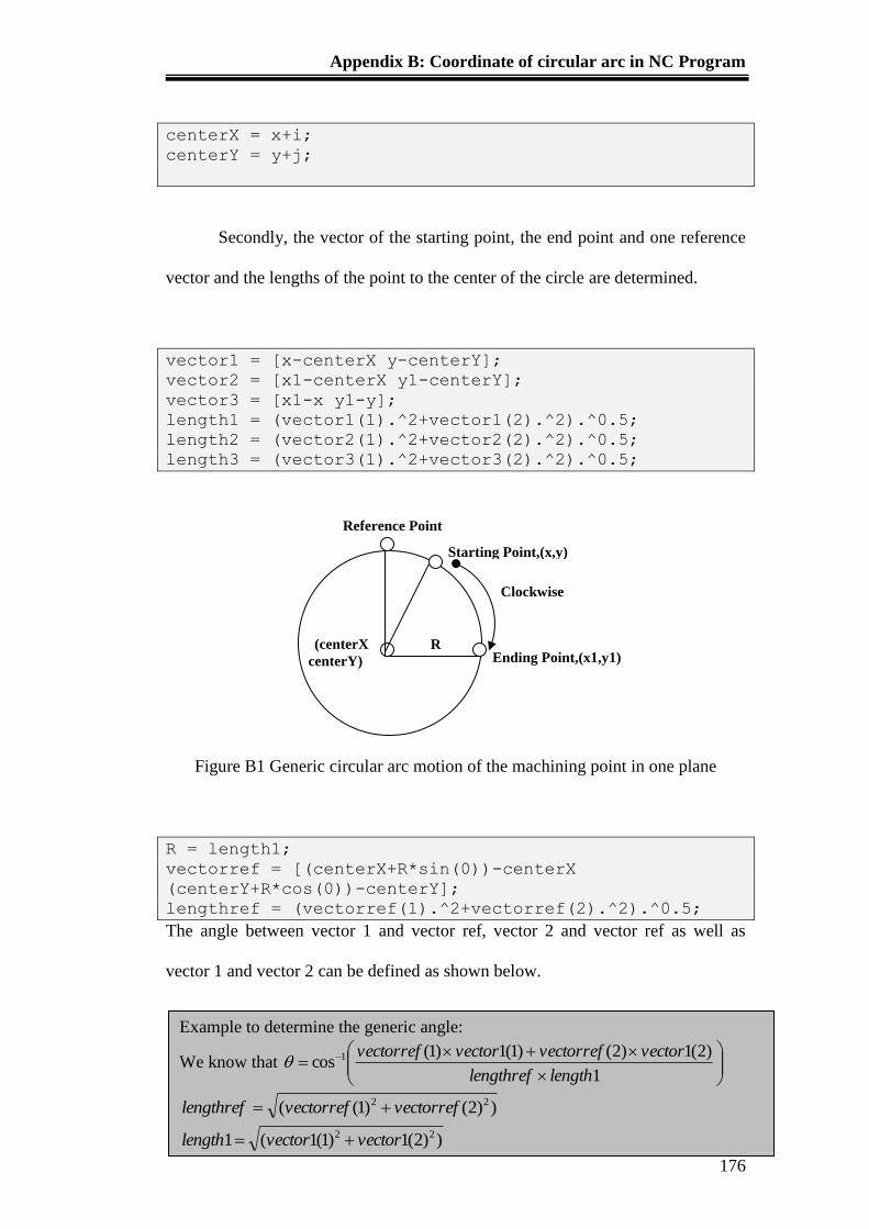
Appendix B: Coordinate of circular arc in NC Program
176
centerX = x+i;
centerY = y+j;
Secondly, the vector of the starting point, the end point and one reference
vector and the lengths of the point to the center of the circle are determined.
vector1 = [x-centerX y-centerY];
vector2 = [x1-centerX y1-centerY];
vector3 = [x1-x y1-y];
length1 = (vector1(1).^2+vector1(2).^2).^0.5;
length2 = (vector2(1).^2+vector2(2).^2).^0.5;
length3 = (vector3(1).^2+vector3(2).^2).^0.5;
Figure B1 Generic circular arc motion of the machining point in one plane
R = length1;
vectorref = [(centerX+R*sin(0))-centerX
(centerY+R*cos(0))-centerY];
lengthref = (vectorref(1).^2+vectorref(2).^2).^0.5;
The angle between vector 1 and vector ref, vector 2 and vector ref as well as
vector 1 and vector 2 can be defined as shown below.
Starting Point,(x,y)
(centerX
centerY) Ending Point,(x1,y1)
Clockwise
R
Reference Point
Example to determine the generic angle:
We know that
1
)2(1)2()1(1)1(cos 1
lengthlengthref
vectorvectorrefvectorvectorref
))2()1(( 22 vectorrefvectorreflengthref
))2(1)1(1(1 22 vectorvectorlength
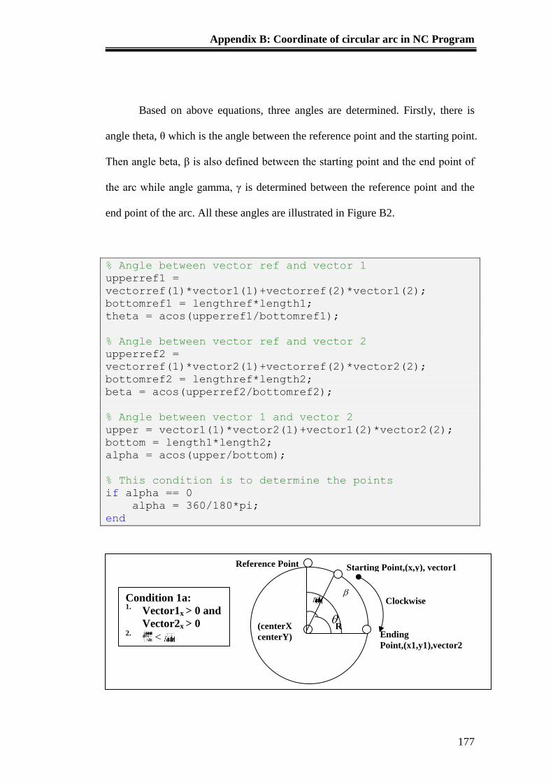
Appendix B: Coordinate of circular arc in NC Program
177
Based on above equations, three angles are determined. Firstly, there is
angle theta, θ which is the angle between the reference point and the starting point.
Then angle beta, β is also defined between the starting point and the end point of
the arc while angle gamma, γ is determined between the reference point and the
end point of the arc. All these angles are illustrated in Figure B2.
% Angle between vector ref and vector 1
upperref1 =
vectorref(1)*vector1(1)+vectorref(2)*vector1(2);
bottomref1 = lengthref*length1;
theta = acos(upperref1/bottomref1);
% Angle between vector ref and vector 2
upperref2 =
vectorref(1)*vector2(1)+vectorref(2)*vector2(2);
bottomref2 = lengthref*length2;
beta = acos(upperref2/bottomref2);
% Angle between vector 1 and vector 2
upper = vector1(1)*vector2(1)+vector1(2)*vector2(2);
bottom = length1*length2;
alpha = acos(upper/bottom);
% This condition is to determine the points
if alpha == 0
alpha = 360/180*pi;
end
Ending
Point,(x1,y1),vector2
Clockwise
Starting Point,(x,y), vector1
(centerX
centerY)
R
Reference Point
Condition 1a: 1.
Vector1x > 0 and
Vector2x > 0
2. <
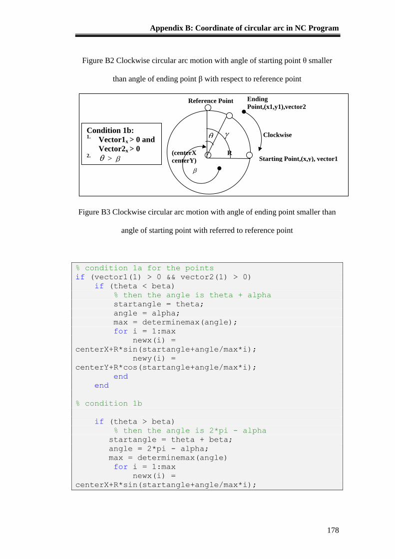
Appendix B: Coordinate of circular arc in NC Program
178
Figure B2 Clockwise circular arc motion with angle of starting point θ smaller
than angle of ending point β with respect to reference point
Figure B3 Clockwise circular arc motion with angle of ending point smaller than
angle of starting point with referred to reference point
% condition 1a for the points
if (vector1(1) > 0 && vector2(1) > 0)
if (theta < beta)
% then the angle is theta + alpha
startangle = theta;
angle = alpha;
max = determinemax(angle);
for i = 1:max
newx(i) =
centerX+R*sin(startangle+angle/max*i);
newy(i) =
centerY+R*cos(startangle+angle/max*i);
end
end
% condition 1b
if (theta > beta)
% then the angle is 2*pi - alpha
startangle = theta + beta;
angle = 2*pi - alpha;
max = determinemax(angle)
for i = 1:max
newx(i) =
centerX+R*sin(startangle+angle/max*i);
Ending
Point,(x1,y1),vector2
Clockwise
Starting Point,(x,y), vector1 (centerX
centerY)
R
Reference Point
Condition 1b: 1.
Vector1x > 0 and
Vector2x > 0
2. >
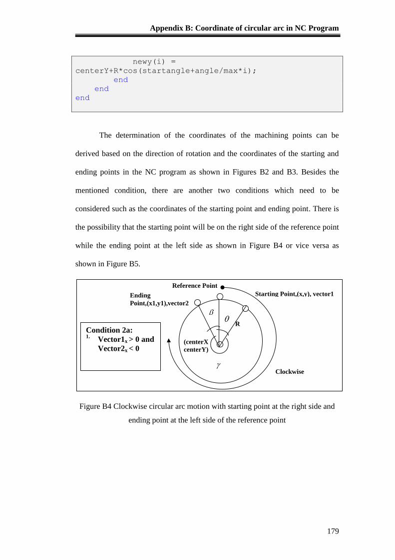
Appendix B: Coordinate of circular arc in NC Program
179
newy(i) =
centerY+R*cos(startangle+angle/max*i);
end
end
end
The determination of the coordinates of the machining points can be
derived based on the direction of rotation and the coordinates of the starting and
ending points in the NC program as shown in Figures B2 and B3. Besides the
mentioned condition, there are another two conditions which need to be
considered such as the coordinates of the starting point and ending point. There is
the possibility that the starting point will be on the right side of the reference point
while the ending point at the left side as shown in Figure B4 or vice versa as
shown in Figure B5.
Figure B4 Clockwise circular arc motion with starting point at the right side and
ending point at the left side of the reference point
Ending
Point,(x1,y1),vector2
Clockwise
Starting Point,(x,y), vector1
(centerX
centerY)
R
Reference Point
Condition 2a: 1.
Vector1x > 0 and
Vector2x < 0
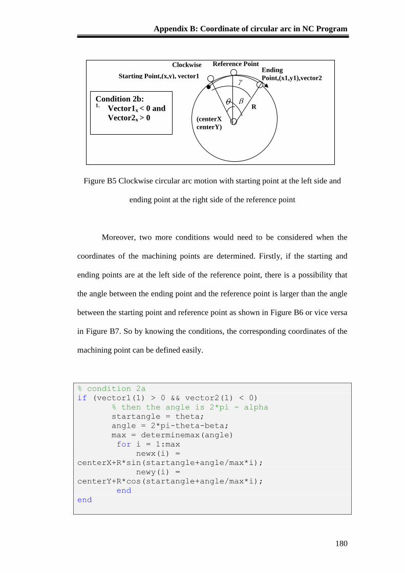
Appendix B: Coordinate of circular arc in NC Program
180
Figure B5 Clockwise circular arc motion with starting point at the left side and
ending point at the right side of the reference point
Moreover, two more conditions would need to be considered when the
coordinates of the machining points are determined. Firstly, if the starting and
ending points are at the left side of the reference point, there is a possibility that
the angle between the ending point and the reference point is larger than the angle
between the starting point and reference point as shown in Figure B6 or vice versa
in Figure B7. So by knowing the conditions, the corresponding coordinates of the
machining point can be defined easily.
% condition 2a
if (vector1(1) > 0 && vector2(1) < 0)
% then the angle is 2*pi - alpha
startangle = theta;
angle = 2*pi-theta-beta;
max = determinemax(angle)
for i = 1:max
newx(i) =
centerX+R*sin(startangle+angle/max*i);
newy(i) =
centerY+R*cos(startangle+angle/max*i);
end
end
Clockwise
Starting Point,(x,y), vector1
(centerX
centerY)
R
Reference Point
Condition 2b: 1.
Vector1x < 0 and
Vector2x > 0
Ending
Point,(x1,y1),vector2
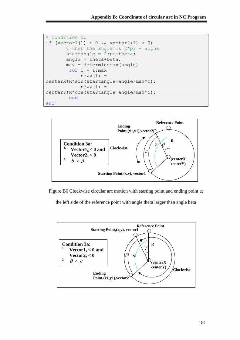
Appendix B: Coordinate of circular arc in NC Program
181
% condition 2b
if (vector1(1) < 0 && vector2(1) > 0)
% then the angle is 2*pi - alpha
startangle = 2*pi-theta;
angle = theta+beta;
max = determinemax(angle)
for i = 1:max
newx(i) =
centerX+R*sin(startangle+angle/max*i);
newy(i) =
centerY+R*cos(startangle+angle/max*i);
end
end
Figure B6 Clockwise circular arc motion with starting point and ending point at
the left side of the reference point with angle theta larger than angle beta
Ending
Point,(x1,y1),vector2
Starting Point,(x,y), vector1
Condition 3a: 1.
Vector1x < 0 and
Vector2x < 0
2. >
Clockwise
(centerX
centerY)
R
Reference Point
Ending
Point,(x1,y1),vector2
Starting Point,(x,y), vector1
Condition 3a: 1.
Vector1x < 0 and
Vector2x < 0
2. <
Clockwise
(centerX
centerY)
R
Reference Point
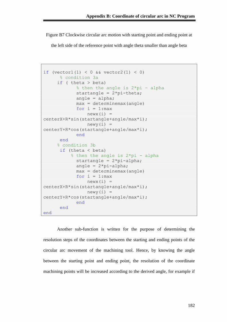
Appendix B: Coordinate of circular arc in NC Program
182
Figure B7 Clockwise circular arc motion with starting point and ending point at
the left side of the reference point with angle theta smaller than angle beta
if (vector1(1) < 0 && vector2(1) < 0)
% condition 3a
if ( theta > beta)
% then the angle is 2*pi - alpha
startangle = 2*pi-theta;
angle = alpha;
max = determinemax(angle)
for i = 1:max
newx(i) =
centerX+R*sin(startangle+angle/max*i);
newy(i) =
centerY+R*cos(startangle+angle/max*i);
end
end
% condition 3b
if (theta < beta)
% then the angle is 2*pi - alpha
startangle = 2*pi-alpha;
angle = 2*pi-alpha;
max = determinemax(angle)
for i = 1:max
newx(i) =
centerX+R*sin(startangle+angle/max*i);
newy(i) =
centerY+R*cos(startangle+angle/max*i);
end
end
end
Another sub-function is written for the purpose of determining the
resolution steps of the coordinates between the starting and ending points of the
circular arc movement of the machining tool. Hence, by knowing the angle
between the starting point and ending point, the resolution of the coordinate
machining points will be increased according to the derived angle, for example if
Appendix B: Coordinate of circular arc in NC Program
183
the angle is smaller than 90° then the resolution of the number of coordinates of
the machining points will be 12.
% Extra function to determine the points along the path
function max = determinemax(angle)
if angle*180/pi <= 90
max = 12
end
if angle*180/pi > 90 && angle*180/pi <= 180
max = 18
end
if angle*180/pi > 180 && angle*180/pi <=270
max = 24
end
if angle*180/pi > 270 && angle*180/pi <=360
max = 30
end
In short, this algorithm can be used to categorize the resolution of the steps
of all the machining coordinates by knowing the starting and ending points of the
circular arc in the NC program. The same conditions and rules can also be applied
to the tool movement in the NC program when it moves in an anticlockwise
direction.
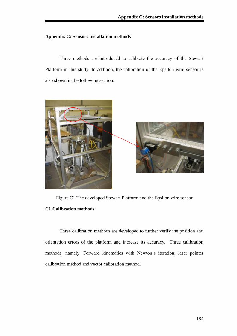
Appendix C: Sensors installation methods
184
Appendix C: Sensors installation methods
Three methods are introduced to calibrate the accuracy of the Stewart
Platform in this study. In addition, the calibration of the Epsilon wire sensor is
also shown in the following section.
Figure C1 The developed Stewart Platform and the Epsilon wire sensor
C1. Calibration methods
Three calibration methods are developed to further verify the position and
orientation errors of the platform and increase its accuracy. Three calibration
methods, namely: Forward kinematics with Newton’s iteration, laser pointer
calibration method and vector calibration method.
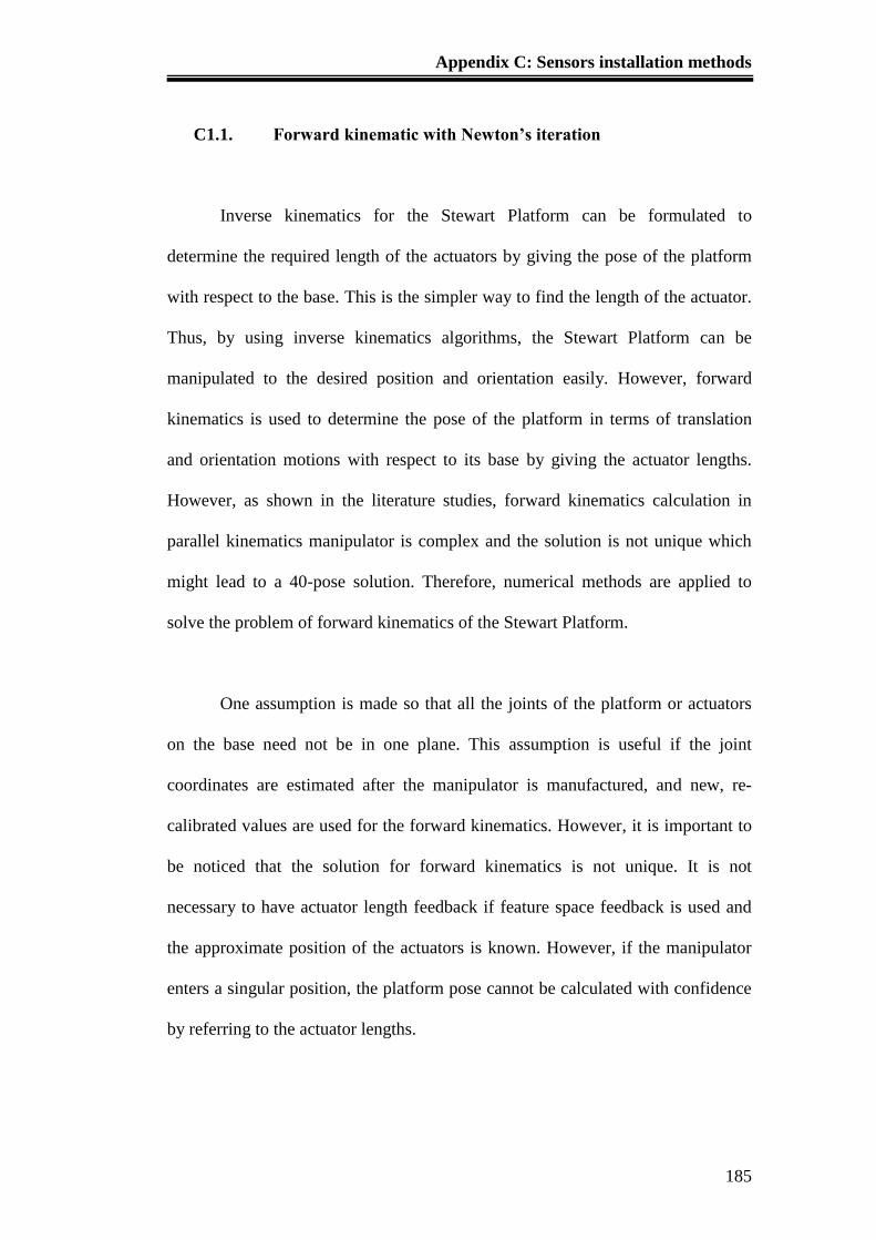
Appendix C: Sensors installation methods
185
C1.1. Forward kinematic with Newton’s iteration
Inverse kinematics for the Stewart Platform can be formulated to
determine the required length of the actuators by giving the pose of the platform
with respect to the base. This is the simpler way to find the length of the actuator.
Thus, by using inverse kinematics algorithms, the Stewart Platform can be
manipulated to the desired position and orientation easily. However, forward
kinematics is used to determine the pose of the platform in terms of translation
and orientation motions with respect to its base by giving the actuator lengths.
However, as shown in the literature studies, forward kinematics calculation in
parallel kinematics manipulator is complex and the solution is not unique which
might lead to a 40-pose solution. Therefore, numerical methods are applied to
solve the problem of forward kinematics of the Stewart Platform.
One assumption is made so that all the joints of the platform or actuators
on the base need not be in one plane. This assumption is useful if the joint
coordinates are estimated after the manipulator is manufactured, and new, re-
calibrated values are used for the forward kinematics. However, it is important to
be noticed that the solution for forward kinematics is not unique. It is not
necessary to have actuator length feedback if feature space feedback is used and
the approximate position of the actuators is known. However, if the manipulator
enters a singular position, the platform pose cannot be calculated with confidence
by referring to the actuator lengths.
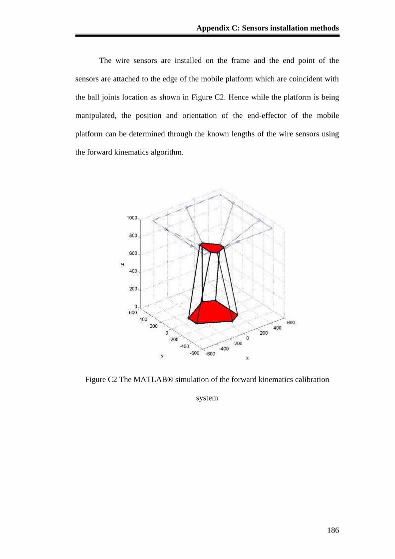
Appendix C: Sensors installation methods
186
The wire sensors are installed on the frame and the end point of the
sensors are attached to the edge of the mobile platform which are coincident with
the ball joints location as shown in Figure C2. Hence while the platform is being
manipulated, the position and orientation of the end-effector of the mobile
platform can be determined through the known lengths of the wire sensors using
the forward kinematics algorithm.
Figure C2 The MATLAB® simulation of the forward kinematics calibration
system
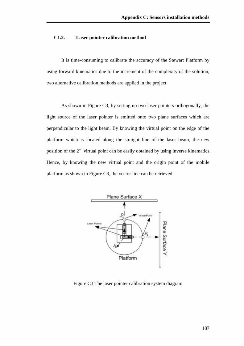
Appendix C: Sensors installation methods
187
C1.2. Laser pointer calibration method
It is time-consuming to calibrate the accuracy of the Stewart Platform by
using forward kinematics due to the increment of the complexity of the solution,
two alternative calibration methods are applied in the project.
As shown in Figure C3, by setting up two laser pointers orthogonally, the
light source of the laser pointer is emitted onto two plane surfaces which are
perpendicular to the light beam. By knowing the virtual point on the edge of the
platform which is located along the straight line of the laser beam, the new
position of the 2nd
virtual point can be easily obtained by using inverse kinematics.
Hence, by knowing the new virtual point and the origin point of the mobile
platform as shown in Figure C3, the vector line can be retrieved.
Figure C3 The laser pointer calibration system diagram
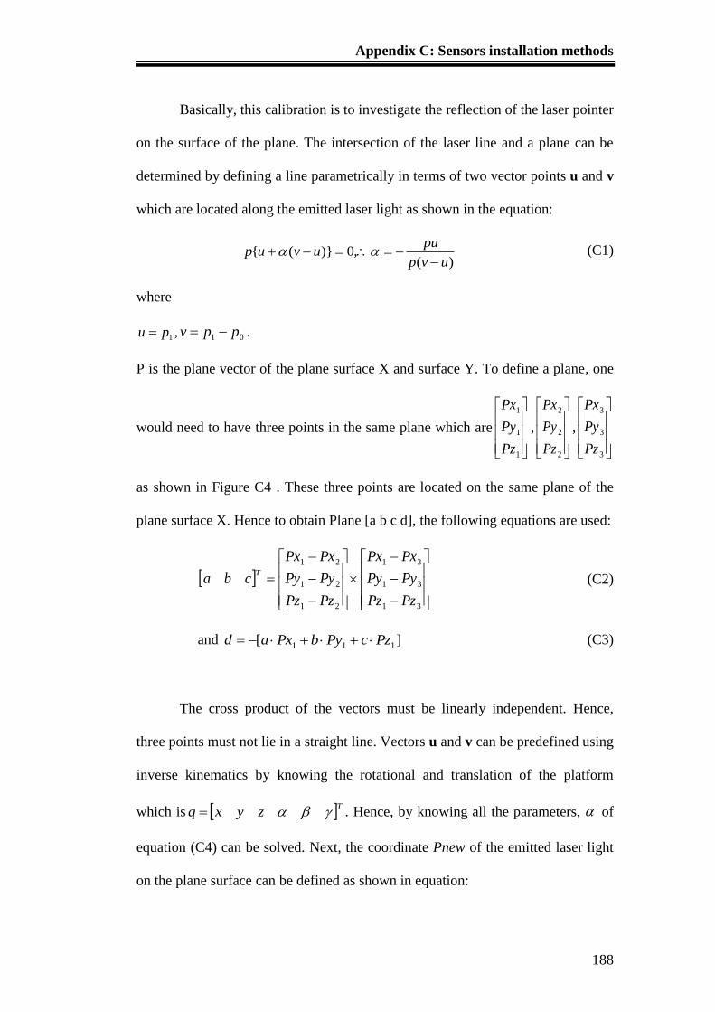
Appendix C: Sensors installation methods
188
Basically, this calibration is to investigate the reflection of the laser pointer
on the surface of the plane. The intersection of the laser line and a plane can be
determined by defining a line parametrically in terms of two vector points u and v
which are located along the emitted laser light as shown in the equation:
)(,0)}({
uvp
puuvup
(C1)
where
1pu , 01 ppv .
P is the plane vector of the plane surface X and surface Y. To define a plane, one
would need to have three points in the same plane which are
1
1
1
Pz
Py
Px
,
2
2
2
Pz
Py
Px
,
3
3
3
Pz
Py
Px
as shown in Figure C4 . These three points are located on the same plane of the
plane surface X. Hence to obtain Plane [a b c d], the following equations are used:
31
31
31
21
21
21
PzPz
PyPy
PxPx
PzPz
PyPy
PxPx
cbaT
(C2)
and ][ 111 PzcPybPxad (C3)
The cross product of the vectors must be linearly independent. Hence,
three points must not lie in a straight line. Vectors u and v can be predefined using
inverse kinematics by knowing the rotational and translation of the platform
which is Tzyxq . Hence, by knowing all the parameters, of
equation (C4) can be solved. Next, the coordinate Pnew of the emitted laser light
on the plane surface can be defined as shown in equation:
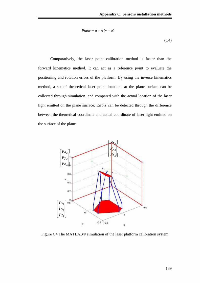
Appendix C: Sensors installation methods
189
)( uvuPnew
(C4)
Comparatively, the laser point calibration method is faster than the
forward kinematics method. It can act as a reference point to evaluate the
positioning and rotation errors of the platform. By using the inverse kinematics
method, a set of theoretical laser point locations at the plane surface can be
collected through simulation, and compared with the actual location of the laser
light emitted on the plane surface. Errors can be detected through the difference
between the theoretical coordinate and actual coordinate of laser light emitted on
the surface of the plane.
Figure C4 The MATLAB® simulation of the laser platform calibration system
1
1
1
Pz
Py
Px
2
2
2
Pz
Py
Px
3
3
3
Pz
Py
Px
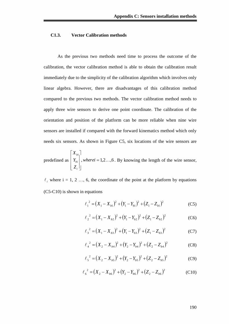
Appendix C: Sensors installation methods
190
C1.3. Vector Calibration methods
As the previous two methods need time to process the outcome of the
calibration, the vector calibration method is able to obtain the calibration result
immediately due to the simplicity of the calibration algorithm which involves only
linear algebra. However, there are disadvantages of this calibration method
compared to the previous two methods. The vector calibration method needs to
apply three wire sensors to derive one point coordinate. The calibration of the
orientation and position of the platform can be more reliable when nine wire
sensors are installed if compared with the forward kinematics method which only
needs six sensors. As shown in Figure C5, six locations of the wire sensors are
predefined as 6,2,1,
wherei
Z
Y
X
i
bi
bi
. By knowing the length of the wire sensor,
i where i = 1, 2 …, 6, the coordinate of the point at the platform by equations
(C5-C10) is shown in equations
211
2
11
2
11
2
1 bbb ZZYYXX (C5)
221
2
21
2
21
2
2 bbb ZZYYXX (C6)
231
2
31
2
31
2
3 bbb ZZYYXX (C7)
242
2
42
2
42
2
4 bbb ZZYYXX (C8)
252
2
52
2
52
2
5 bbb ZZYYXX (C9)
262
2
62
2
62
2
6 bbb ZZYYXX (C10)
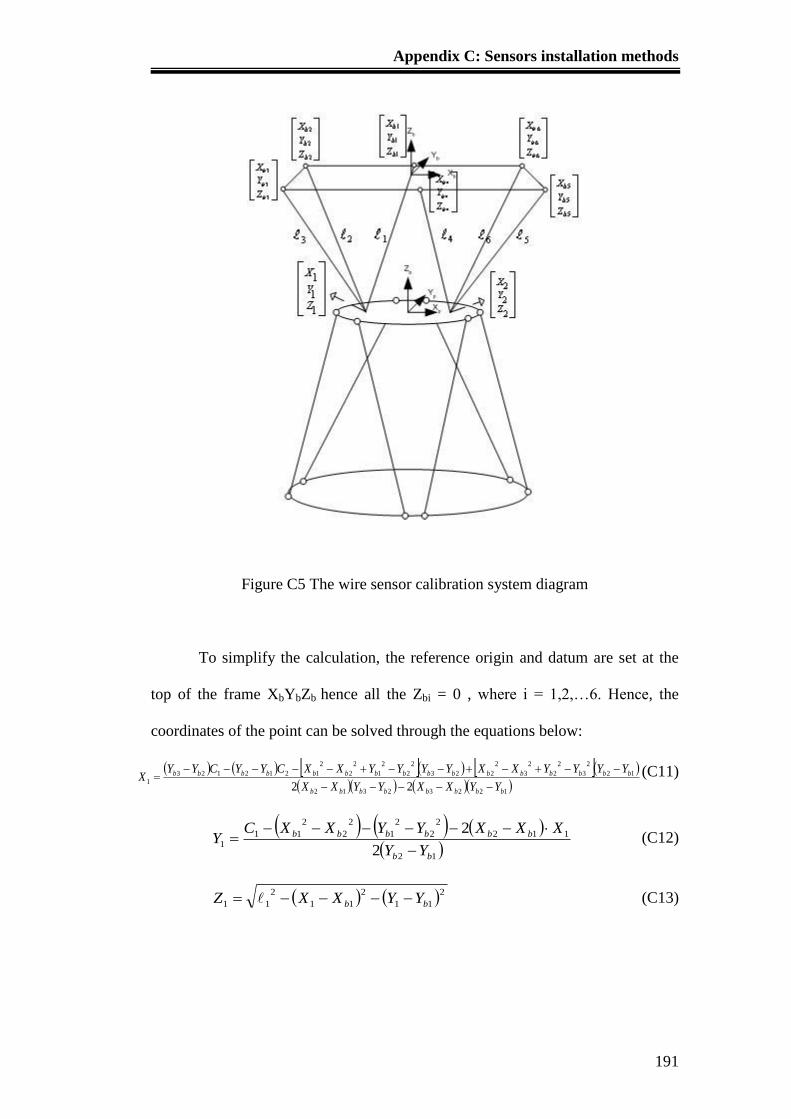
Appendix C: Sensors installation methods
191
Figure C5 The wire sensor calibration system diagram
To simplify the calculation, the reference origin and datum are set at the
top of the frame XbYbZb hence all the Zbi = 0 , where i = 1,2,…6. Hence, the
coordinates of the point can be solved through the equations below:
12232312
12
2
3
2
2
2
3
2
223
2
2
2
1
2
2
2
12121231
22 bbbbbbbb
bbbbbbbbbbbbbbbb
YYXXYYXX
YYYYXXYYYYXXCYYCYYX
(C11)
12
112
2
2
2
1
2
2
2
111
2
2
bb
bbbbbb
YY
XXXYYXXCY
(C12)
2
11
2
11
2
11 bb YYXXZ (C13)
Appendix C: Sensors installation methods
192
where 2
2
2
11 C , 2
3
2
22 C . Hence similarly, matrix
2
2
2
Z
Y
X
can be
obtained by using the same method of Equations (C11), (C12) and (C13).
Therefore, by acquiring values from the three wire sensors, the position of the
platform can be evaluated. However, it could only specify the position of the
platform. The definition of the orientation of the platform can only be achieved
when three vector points are defined on the surface of the platform. The
coordinate of the vector points can be used to form a vector plane which allows
the orientation of the platform to be read with respect to the reference plane.
However, this configuration of the system requires at least nine sensors. Since
only six wire sensors are available, an alternative method is applied to acquire the
desired position and orientation. Six wires are attached to two points on the
surface of the platform as shown in Figure C6. The locations of the points are
predefined such that two of the points are of equal distance and aligned with the
center point of the platform. Thus, the center of the platform
C
C
C
Z
Y
X
can be
acquired by a simple equation in Equation (C14).
2
21 XXX C
,
Y
YYYC
21 ,2
21 ZZZC
(C14)
To determine the orientation of the platform, a geometric method is used
to measure the angle of rotation of the platform, roll-pitch-yaw: , and as
shown in Figure C6.
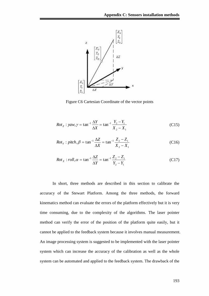
Appendix C: Sensors installation methods
193
Figure C6 Cartesian Coordinate of the vector points
12
1211 tantan,:XX
YY
X
YyawRotZ
(C15)
12
1211 tantan,:XX
ZZ
X
ZpitchRotY
(C16)
12
1211 tantan,:YY
ZZ
Y
ZrollRot X
(C17)
In short, three methods are described in this section to calibrate the
accuracy of the Stewart Platform. Among the three methods, the forward
kinematics method can evaluate the errors of the platform effectively but it is very
time consuming, due to the complexity of the algorithms. The laser pointer
method can verify the error of the position of the platform quite easily, but it
cannot be applied to the feedback system because it involves manual measurement.
An image processing system is suggested to be implemented with the laser pointer
system which can increase the accuracy of the calibration as well as the whole
system can be automated and applied to the feedback system. The drawback of the
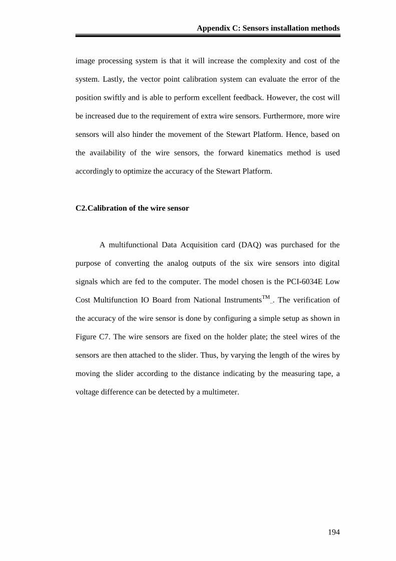
Appendix C: Sensors installation methods
194
image processing system is that it will increase the complexity and cost of the
system. Lastly, the vector point calibration system can evaluate the error of the
position swiftly and is able to perform excellent feedback. However, the cost will
be increased due to the requirement of extra wire sensors. Furthermore, more wire
sensors will also hinder the movement of the Stewart Platform. Hence, based on
the availability of the wire sensors, the forward kinematics method is used
accordingly to optimize the accuracy of the Stewart Platform.
C2. Calibration of the wire sensor
A multifunctional Data Acquisition card (DAQ) was purchased for the
purpose of converting the analog outputs of the six wire sensors into digital
signals which are fed to the computer. The model chosen is the PCI-6034E Low
Cost Multifunction IO Board from National InstrumentsTM
... The verification of
the accuracy of the wire sensor is done by configuring a simple setup as shown in
Figure C7. The wire sensors are fixed on the holder plate; the steel wires of the
sensors are then attached to the slider. Thus, by varying the length of the wires by
moving the slider according to the distance indicating by the measuring tape, a
voltage difference can be detected by a multimeter.
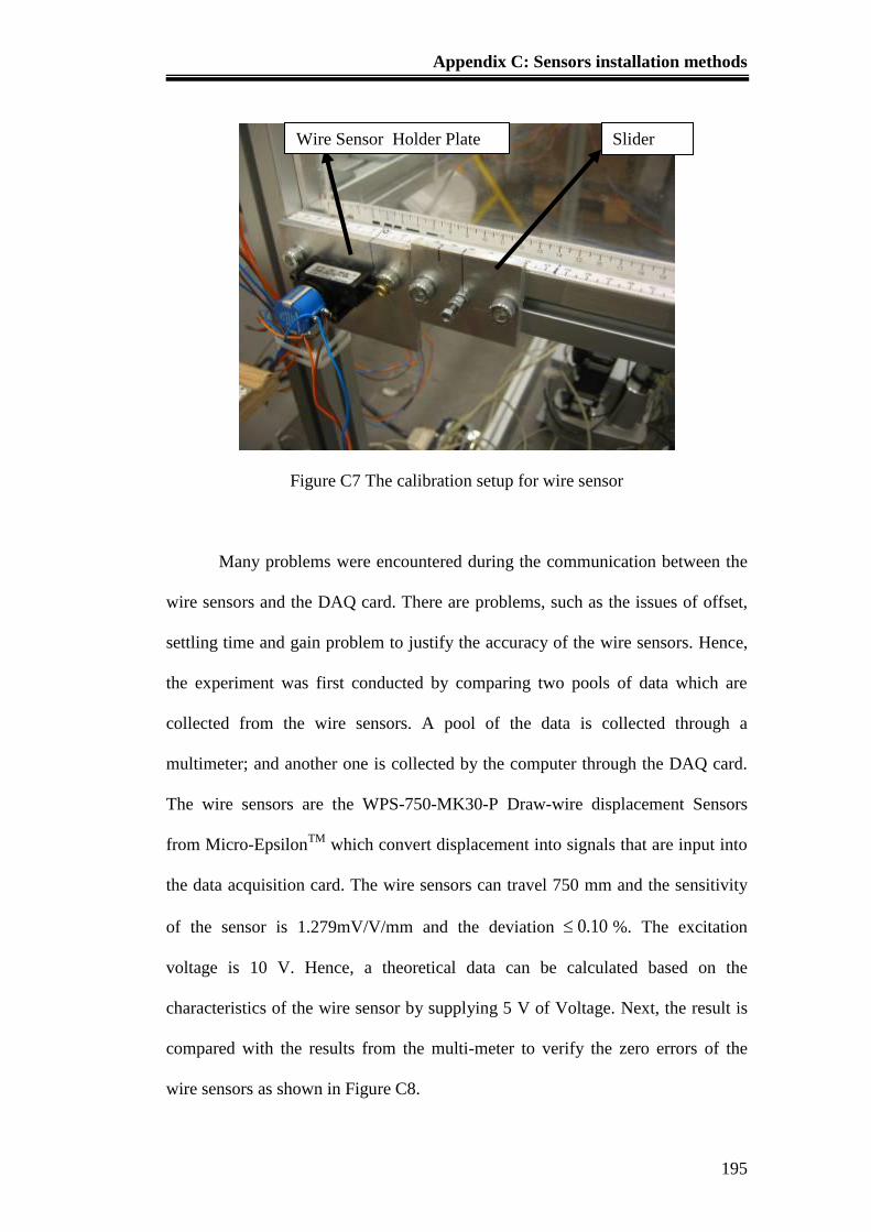
Appendix C: Sensors installation methods
195
Figure C7 The calibration setup for wire sensor
Many problems were encountered during the communication between the
wire sensors and the DAQ card. There are problems, such as the issues of offset,
settling time and gain problem to justify the accuracy of the wire sensors. Hence,
the experiment was first conducted by comparing two pools of data which are
collected from the wire sensors. A pool of the data is collected through a
multimeter; and another one is collected by the computer through the DAQ card.
The wire sensors are the WPS-750-MK30-P Draw-wire displacement Sensors
from Micro-EpsilonTM
which convert displacement into signals that are input into
the data acquisition card. The wire sensors can travel 750 mm and the sensitivity
of the sensor is 1.279mV/V/mm and the deviation 10.0 %. The excitation
voltage is 10 V. Hence, a theoretical data can be calculated based on the
characteristics of the wire sensor by supplying 5 V of Voltage. Next, the result is
compared with the results from the multi-meter to verify the zero errors of the
wire sensors as shown in Figure C8.
Slider Wire Sensor Holder Plate
Appendix C: Sensors installation methods
196
Figure C8 Graph of Comparison between theoretical data and actual data from
Multimeter
From Figure C8, it is noticed that the error between the actual and
theoretical data of wire sensor is minor. It is observed that there is still some offset
at the start of the measurement. The offset problem might be caused by the
settling time or the delay of the signal transfer from the card to the computer.
However, the data collected from the multimeter can be used as a reference data to
verify of the accuracy of the acquired data from the computer. By using Labview
to acquire the data of the wire sensor, an estimated offset of 0.5 V was discovered
as shown in Figure C9. From the graph, the results of the Labview data are
affected by the improper gain setting and sampling rate.
Length Vs Voltage
0
100
200
300
400
500
600
700
800
900
0 1 2 3 4 5 6
Voltage(V)
Len
gth
(mm
)
Voltage vs Length(Theorectical)
Voltage vs Length(Actual)
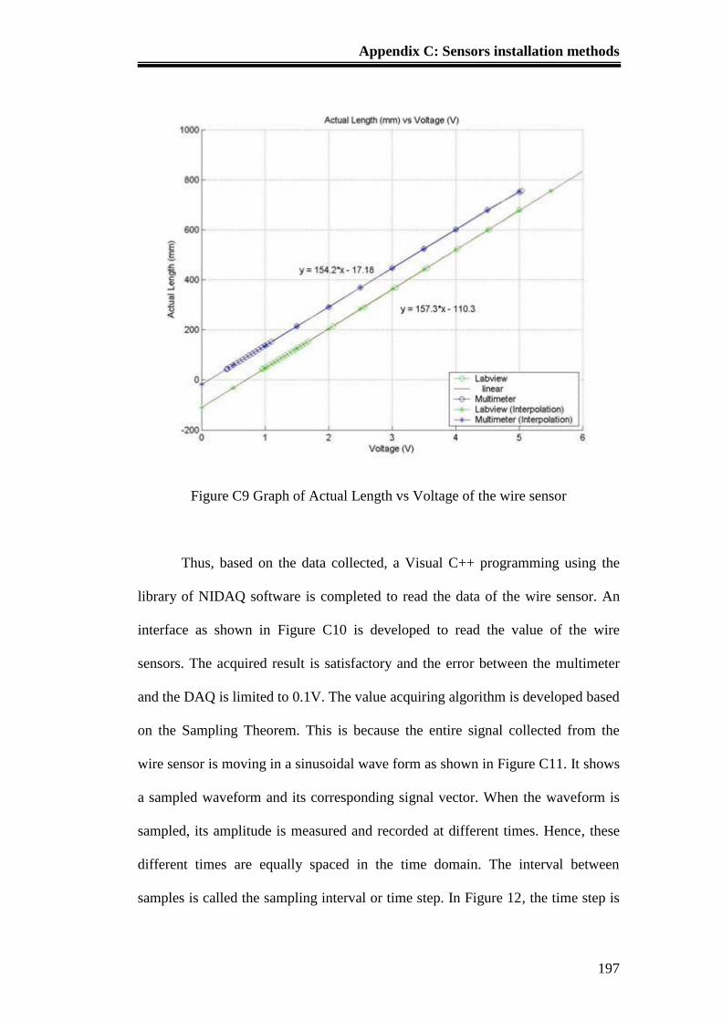
Appendix C: Sensors installation methods
197
Figure C9 Graph of Actual Length vs Voltage of the wire sensor
Thus, based on the data collected, a Visual C++ programming using the
library of NIDAQ software is completed to read the data of the wire sensor. An
interface as shown in Figure C10 is developed to read the value of the wire
sensors. The acquired result is satisfactory and the error between the multimeter
and the DAQ is limited to 0.1V. The value acquiring algorithm is developed based
on the Sampling Theorem. This is because the entire signal collected from the
wire sensor is moving in a sinusoidal wave form as shown in Figure C11. It shows
a sampled waveform and its corresponding signal vector. When the waveform is
sampled, its amplitude is measured and recorded at different times. Hence, these
different times are equally spaced in the time domain. The interval between
samples is called the sampling interval or time step. In Figure 12, the time step is

Appendix C: Sensors installation methods
198
msTt 10 . Thus, to read an average value of the wire sensor, an averaging
method is used.
T
TV
V T
500
1
)(
(C18)
Figure C10 Wire sensor interface
Figure C11 The Sampled Wave Signal of the wire sensors
Voltage vs Time
-0.1
0
0.1
0.2
0.3
0.4
0.5
0.6
0 200 400 600 800 1000 1200
x10ms
Vo
ltag
e(v)
Series1
Series2
Series3
Series4
Series5
Series6
Avg Series Sensor 1
Avg Series Sensor 2
Averaging Sensor 3
Avg Series Sensor 4
Avg Series Sensor 5
Avg series Sensor 6
Poly. (Avg Series Sensor 1)
Poly. (Avg Series Sensor 2)
Poly. (Averaging Sensor 3)
Poly. (Avg Series Sensor 4)
Poly. (Avg Series Sensor 5)
Poly. (Avg series Sensor 6)

Appendix C: Sensors installation methods
199
Hence, by reading the average value, a constant value of the wire sensor
can be obtained as a straight line as shown in Figure C11. After the averaging of
the data, the wire sensors are calibrated and can be used in the calibration systems
mentioned in the previous section to verify the position and orientation of the
Stewart Platform.
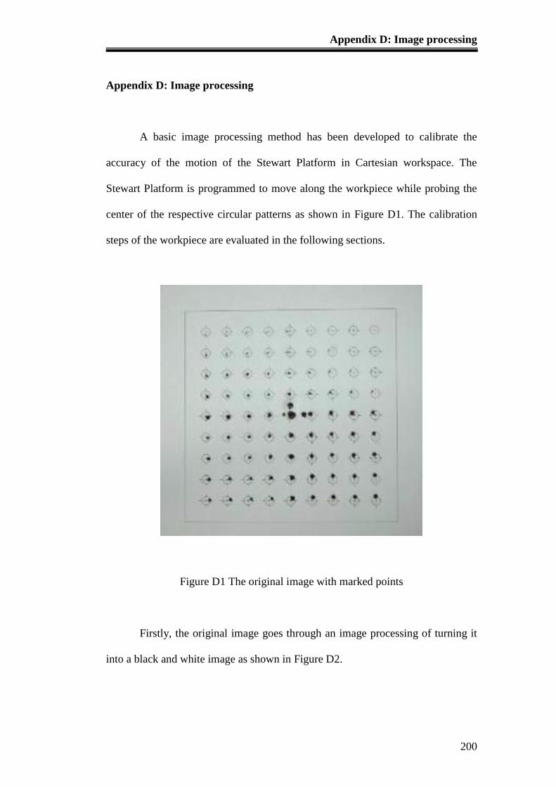
Appendix D: Image processing
200
Appendix D: Image processing
A basic image processing method has been developed to calibrate the
accuracy of the motion of the Stewart Platform in Cartesian workspace. The
Stewart Platform is programmed to move along the workpiece while probing the
center of the respective circular patterns as shown in Figure D1. The calibration
steps of the workpiece are evaluated in the following sections.
Figure D1 The original image with marked points
Firstly, the original image goes through an image processing of turning it
into a black and white image as shown in Figure D2.
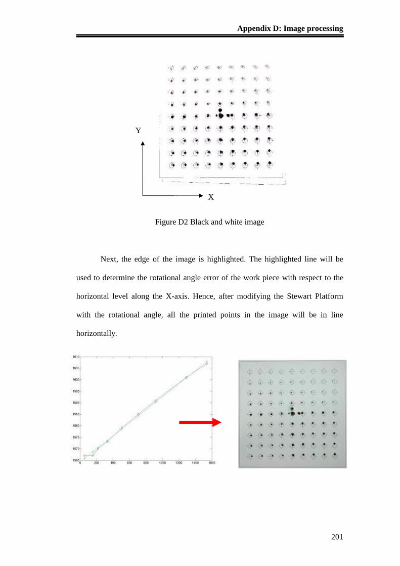
Appendix D: Image processing
201
Figure D2 Black and white image
Next, the edge of the image is highlighted. The highlighted line will be
used to determine the rotational angle error of the work piece with respect to the
horizontal level along the X-axis. Hence, after modifying the Stewart Platform
with the rotational angle, all the printed points in the image will be in line
horizontally.
X
Y
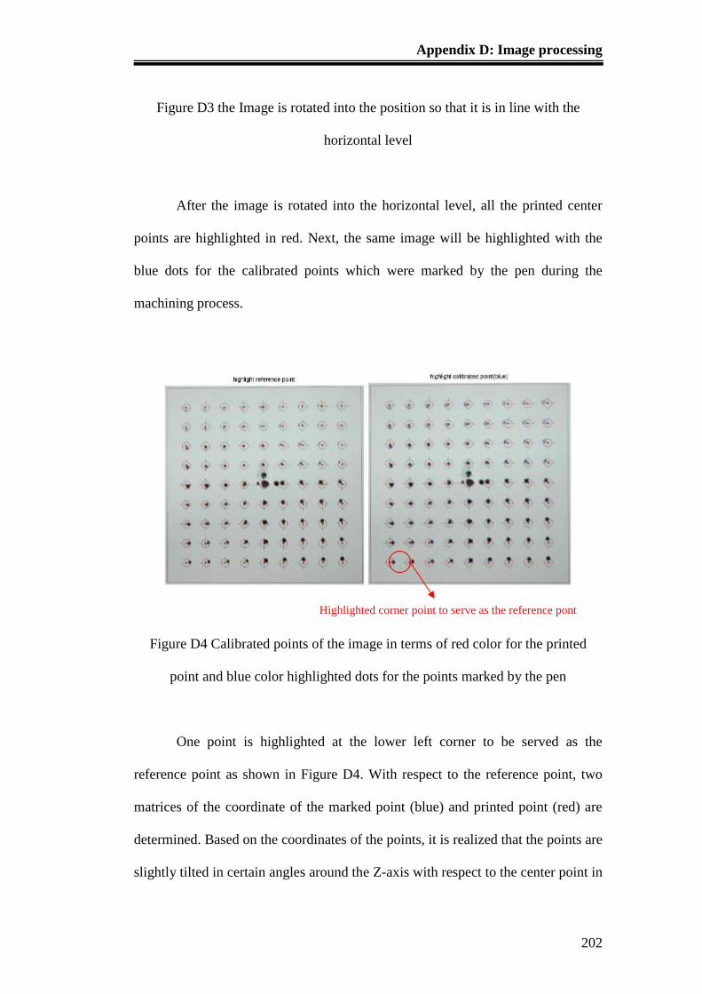
Appendix D: Image processing
202
Figure D3 the Image is rotated into the position so that it is in line with the
horizontal level
After the image is rotated into the horizontal level, all the printed center
points are highlighted in red. Next, the same image will be highlighted with the
blue dots for the calibrated points which were marked by the pen during the
machining process.
Figure D4 Calibrated points of the image in terms of red color for the printed
point and blue color highlighted dots for the points marked by the pen
One point is highlighted at the lower left corner to be served as the
reference point as shown in Figure D4. With respect to the reference point, two
matrices of the coordinate of the marked point (blue) and printed point (red) are
determined. Based on the coordinates of the points, it is realized that the points are
slightly tilted in certain angles around the Z-axis with respect to the center point in
Highlighted corner point to serve as the reference pont
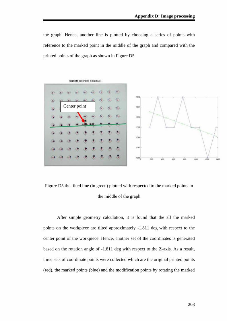
Appendix D: Image processing
203
the graph. Hence, another line is plotted by choosing a series of points with
reference to the marked point in the middle of the graph and compared with the
printed points of the graph as shown in Figure D5.
Figure D5 the tilted line (in green) plotted with respected to the marked points in
the middle of the graph
After simple geometry calculation, it is found that the all the marked
points on the workpiece are tilted approximately -1.811 deg with respect to the
center point of the workpiece. Hence, another set of the coordinates is generated
based on the rotation angle of -1.811 deg with respect to the Z-axis. As a result,
three sets of coordinate points were collected which are the original printed points
(red), the marked points (blue) and the modification points by rotating the marked
Center point

Appendix D: Image processing
204
points around the Z-axis with respect to the middle point of the workpiece (green).
All the coordinates are shown in Figure D6.
From the view of the image of Figure D6, one can see that the error of the
coordinate of the points was reduced when the points were rotated to the positions
as shown in the green spot.
Figure D6a All three sets of coordinates of the Printed Points (Red), Marked
Points (Blue) and Modified Points (Green)
* reference point
○calibrated point
○modified calibrated point by
rotating around Z-axis with
respect to the center point
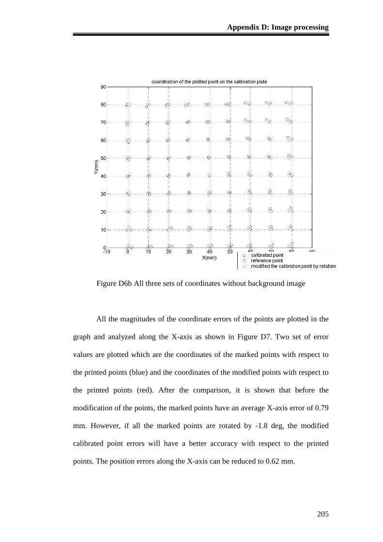
Appendix D: Image processing
205
Figure D6b All three sets of coordinates without background image
All the magnitudes of the coordinate errors of the points are plotted in the
graph and analyzed along the X-axis as shown in Figure D7. Two set of error
values are plotted which are the coordinates of the marked points with respect to
the printed points (blue) and the coordinates of the modified points with respect to
the printed points (red). After the comparison, it is shown that before the
modification of the points, the marked points have an average X-axis error of 0.79
mm. However, if all the marked points are rotated by -1.8 deg, the modified
calibrated point errors will have a better accuracy with respect to the printed
points. The position errors along the X-axis can be reduced to 0.62 mm.
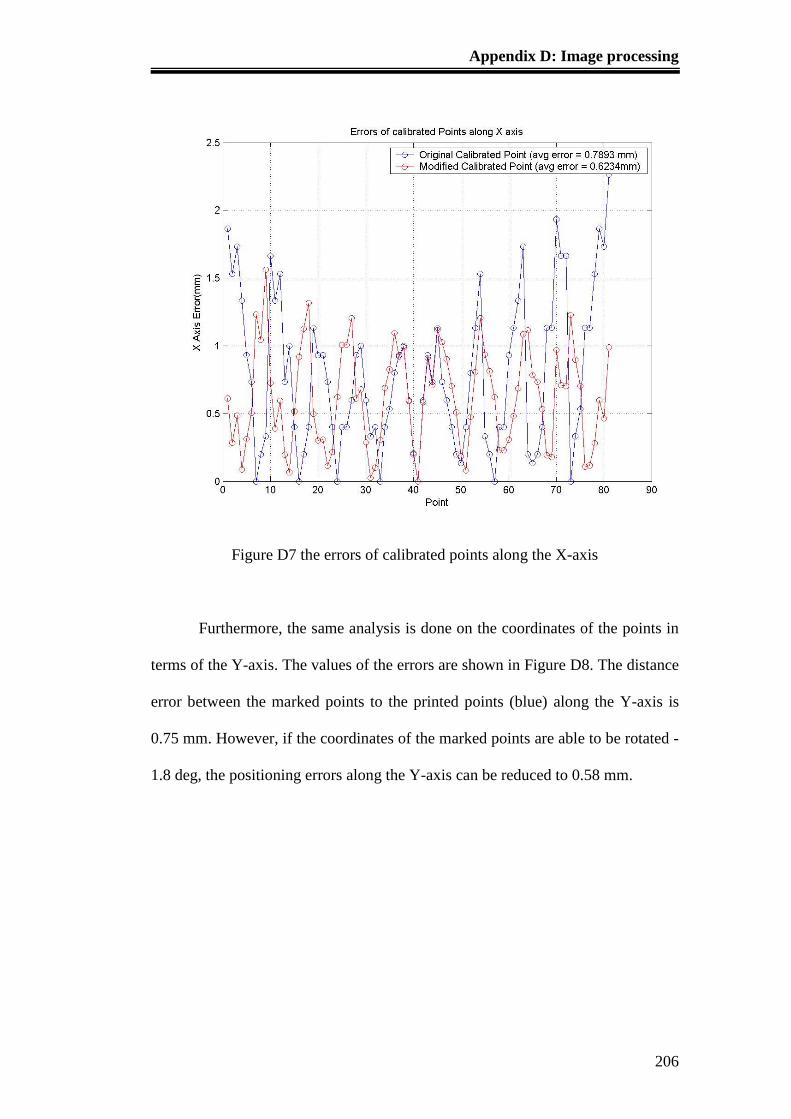
Appendix D: Image processing
206
Figure D7 the errors of calibrated points along the X-axis
Furthermore, the same analysis is done on the coordinates of the points in
terms of the Y-axis. The values of the errors are shown in Figure D8. The distance
error between the marked points to the printed points (blue) along the Y-axis is
0.75 mm. However, if the coordinates of the marked points are able to be rotated -
1.8 deg, the positioning errors along the Y-axis can be reduced to 0.58 mm.
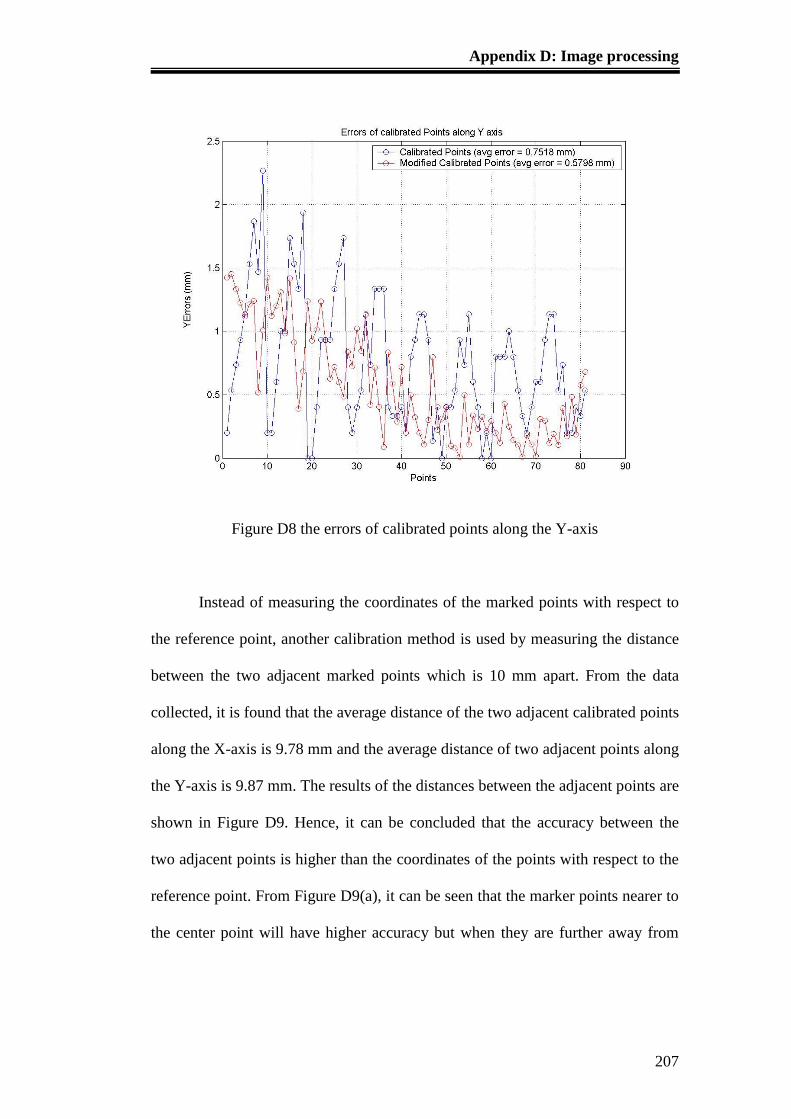
Appendix D: Image processing
207
Figure D8 the errors of calibrated points along the Y-axis
Instead of measuring the coordinates of the marked points with respect to
the reference point, another calibration method is used by measuring the distance
between the two adjacent marked points which is 10 mm apart. From the data
collected, it is found that the average distance of the two adjacent calibrated points
along the X-axis is 9.78 mm and the average distance of two adjacent points along
the Y-axis is 9.87 mm. The results of the distances between the adjacent points are
shown in Figure D9. Hence, it can be concluded that the accuracy between the
two adjacent points is higher than the coordinates of the points with respect to the
reference point. From Figure D9(a), it can be seen that the marker points nearer to
the center point will have higher accuracy but when they are further away from
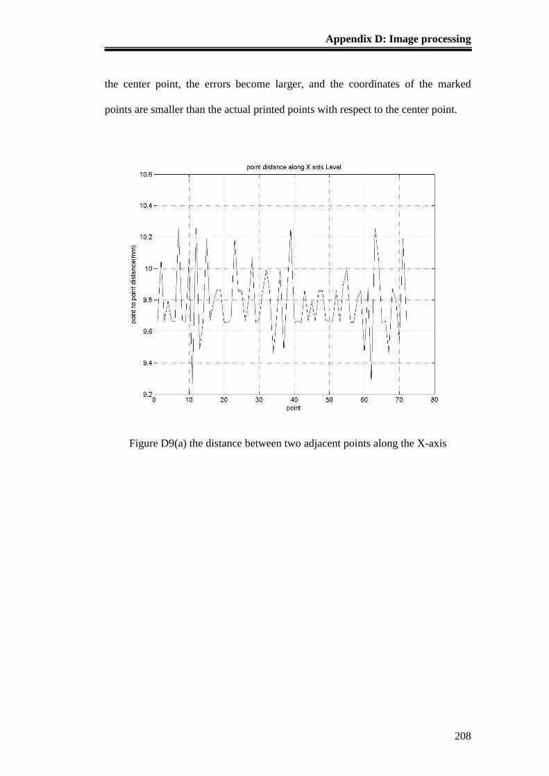
Appendix D: Image processing
208
the center point, the errors become larger, and the coordinates of the marked
points are smaller than the actual printed points with respect to the center point.
Figure D9(a) the distance between two adjacent points along the X-axis
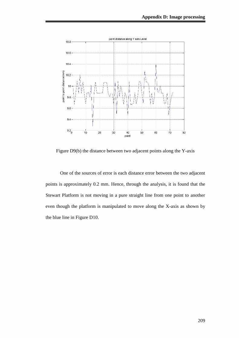
Appendix D: Image processing
209
Figure D9(b) the distance between two adjacent points along the Y-axis
One of the sources of error is each distance error between the two adjacent
points is approximately 0.2 mm. Hence, through the analysis, it is found that the
Stewart Platform is not moving in a pure straight line from one point to another
even though the platform is manipulated to move along the X-axis as shown by
the blue line in Figure D10.
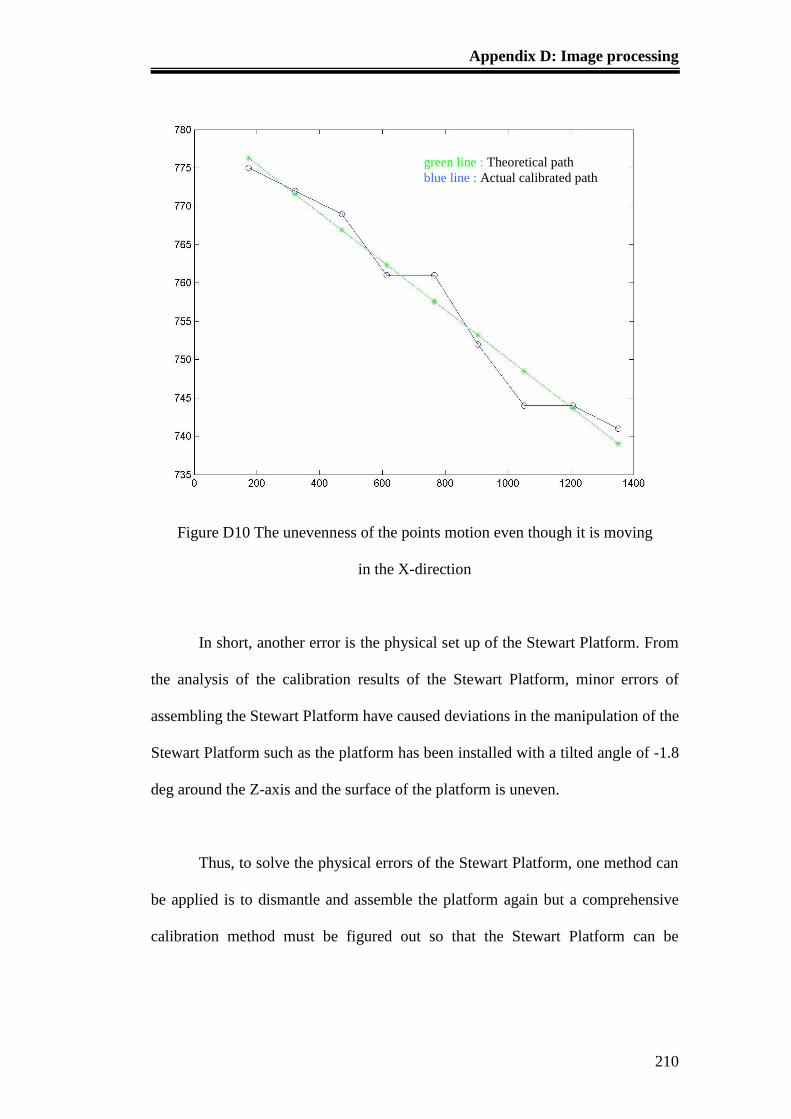
Appendix D: Image processing
210
Figure D10 The unevenness of the points motion even though it is moving
in the X-direction
In short, another error is the physical set up of the Stewart Platform. From
the analysis of the calibration results of the Stewart Platform, minor errors of
assembling the Stewart Platform have caused deviations in the manipulation of the
Stewart Platform such as the platform has been installed with a tilted angle of -1.8
deg around the Z-axis and the surface of the platform is uneven.
Thus, to solve the physical errors of the Stewart Platform, one method can
be applied is to dismantle and assemble the platform again but a comprehensive
calibration method must be figured out so that the Stewart Platform can be
green line : Theoretical path
blue line : Actual calibrated path
Appendix D: Image processing
211
reassembled in a more accurate manner. An alternative method is to compensate
the error by modifying the parameters using software.
The Calibration Experiment
The purpose of this calibration experiment is to fine tune the accuracy of
the Stewart Platform by using the parameters obtained through the analysis of the
processed images. Firstly, the Stewart Platform was turned around the Z-axis by -
1.8 deg. Then the Stewart Platform is turned around rotation about the Y-axis by -
0.5 deg.
After the sensors are verified and rounded to 0.15 mm resolution, all the
wire sensors are installed along the actuators. First of all, by performing the
calibration of single actuator several times, such as every 100,000 counts of the
motor pulse, it moves 145.62 mm – 138.01 mm = 7.61 mm. Hence, a coefficient
of 100000/7.61 is used for the stroke of the Stewart Platform during the
calculation from distance movement to the count of steps of the actuator. As a
result, by assuming a different reachable distance for the actuator to move in
100,000 counts, a graph of errors is plotted based on the calibrated length with the
reference length is shown in Figure D11.
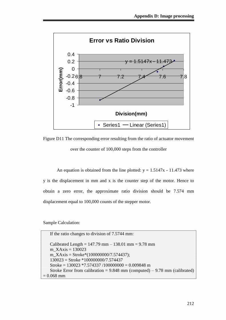
Appendix D: Image processing
212
Figure D11 The corresponding error resulting from the ratio of actuator movement
over the counter of 100,000 steps from the controller
An equation is obtained from the line plotted: y = 1.5147x - 11.473 where
y is the displacement in mm and x is the counter step of the motor. Hence to
obtain a zero error, the approximate ratio division should be 7.574 mm
displacement equal to 100,000 counts of the stepper motor.
Sample Calculation:
If the ratio changes to division of 7.5744 mm:
Calibrated Length = 147.79 mm – 138.01 mm = 9.78 mm
m_XAxis = 130023
m_XAxis = Stroke*(100000000/7.574437);
130023 = Stroke *100000000/7.574437
Stroke = 130023 *7.574337 /100000000 = 0.009848 m
Stroke Error from calibration = 9.848 mm (computed) – 9.78 mm (calibrated)
= 0.068 mm
Error vs Ratio Division
y = 1.5147x - 11.473
-1
-0.8
-0.6
-0.4
-0.2
0
0.2
0.4
6.8 7 7.2 7.4 7.6 7.8
Division(mm)
Err
or(
mm
)
Series1 Linear (Series1)
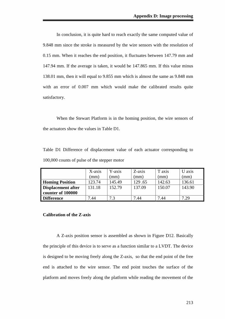
Appendix D: Image processing
213
In conclusion, it is quite hard to reach exactly the same computed value of
9.848 mm since the stroke is measured by the wire sensors with the resolution of
0.15 mm. When it reaches the end position, it fluctuates between 147.79 mm and
147.94 mm. If the average is taken, it would be 147.865 mm. If this value minus
138.01 mm, then it will equal to 9.855 mm which is almost the same as 9.848 mm
with an error of 0.007 mm which would make the calibrated results quite
satisfactory.
When the Stewart Platform is in the homing position, the wire sensors of
the actuators show the values in Table D1.
Table D1 Difference of displacement value of each actuator corresponding to
100,000 counts of pulse of the stepper motor
X-axis
(mm)
Y-axis
(mm)
Z-axis
(mm)
T axis
(mm)
U axis
(mm)
Homing Position 123.74 145.49 129 .65 142.63 136.61
Displacement after
counter of 100000
131.18 152.79 137.09 150.07 143.90
Difference 7.44 7.3 7.44 7.44 7.29
Calibration of the Z-axis
A Z-axis position sensor is assembled as shown in Figure D12. Basically
the principle of this device is to serve as a function similar to a LVDT. The device
is designed to be moving freely along the Z-axis, so that the end point of the free
end is attached to the wire sensor. The end point touches the surface of the
platform and moves freely along the platform while reading the movement of the
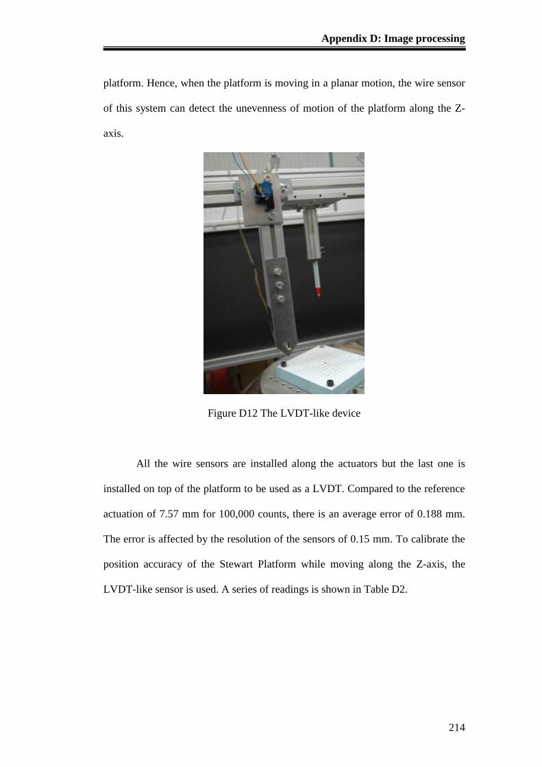
Appendix D: Image processing
214
platform. Hence, when the platform is moving in a planar motion, the wire sensor
of this system can detect the unevenness of motion of the platform along the Z-
axis.
Figure D12 The LVDT-like device
All the wire sensors are installed along the actuators but the last one is
installed on top of the platform to be used as a LVDT. Compared to the reference
actuation of 7.57 mm for 100,000 counts, there is an average error of 0.188 mm.
The error is affected by the resolution of the sensors of 0.15 mm. To calibrate the
position accuracy of the Stewart Platform while moving along the Z-axis, the
LVDT-like sensor is used. A series of readings is shown in Table D2.
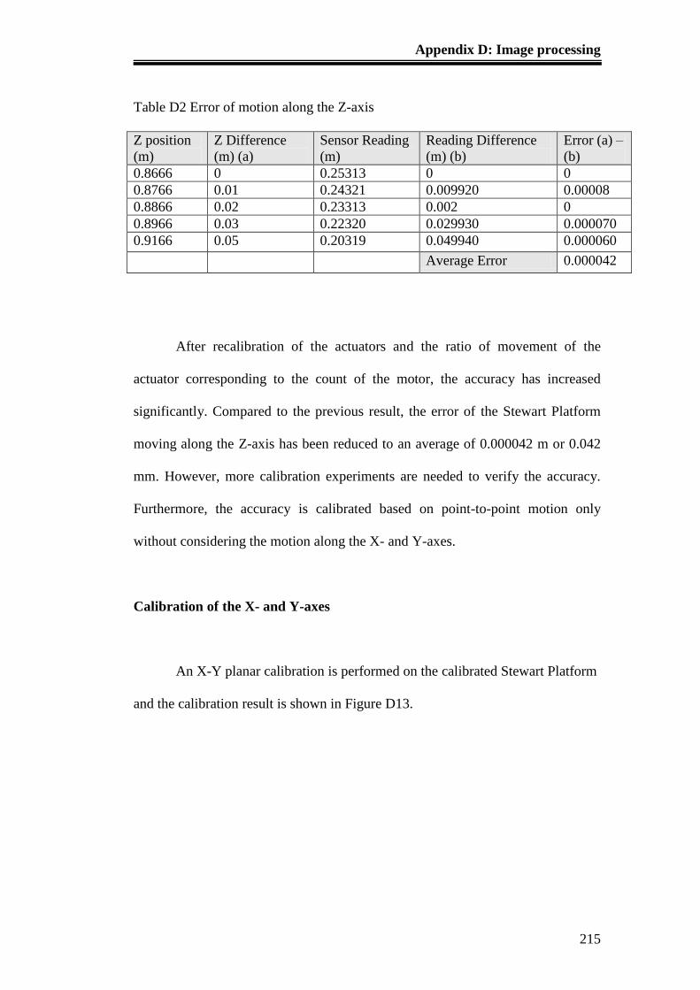
Appendix D: Image processing
215
Table D2 Error of motion along the Z-axis
Z position
(m)
Z Difference
(m) (a)
Sensor Reading
(m)
Reading Difference
(m) (b)
Error (a) –
(b)
0.8666 0 0.25313 0 0
0.8766 0.01 0.24321 0.009920 0.00008
0.8866 0.02 0.23313 0.002 0
0.8966 0.03 0.22320 0.029930 0.000070
0.9166 0.05 0.20319 0.049940 0.000060
Average Error 0.000042
After recalibration of the actuators and the ratio of movement of the
actuator corresponding to the count of the motor, the accuracy has increased
significantly. Compared to the previous result, the error of the Stewart Platform
moving along the Z-axis has been reduced to an average of 0.000042 m or 0.042
mm. However, more calibration experiments are needed to verify the accuracy.
Furthermore, the accuracy is calibrated based on point-to-point motion only
without considering the motion along the X- and Y-axes.
Calibration of the X- and Y-axes
An X-Y planar calibration is performed on the calibrated Stewart Platform
and the calibration result is shown in Figure D13.
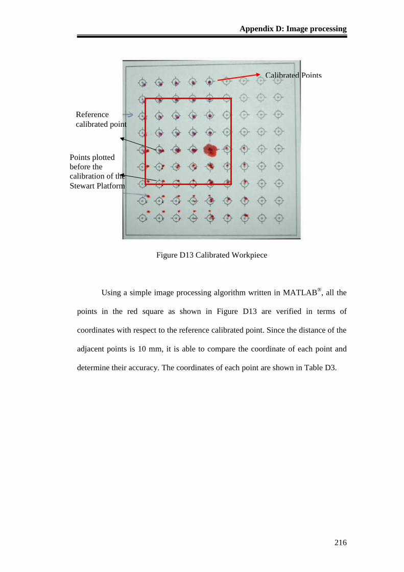
Appendix D: Image processing
216
Figure D13 Calibrated Workpiece
Using a simple image processing algorithm written in MATLAB®, all the
points in the red square as shown in Figure D13 are verified in terms of
coordinates with respect to the reference calibrated point. Since the distance of the
adjacent points is 10 mm, it is able to compare the coordinate of each point and
determine their accuracy. The coordinates of each point are shown in Table D3.
Reference
calibrated point
Points plotted
before the
calibration of the
Stewart Platform
Calibrated Points
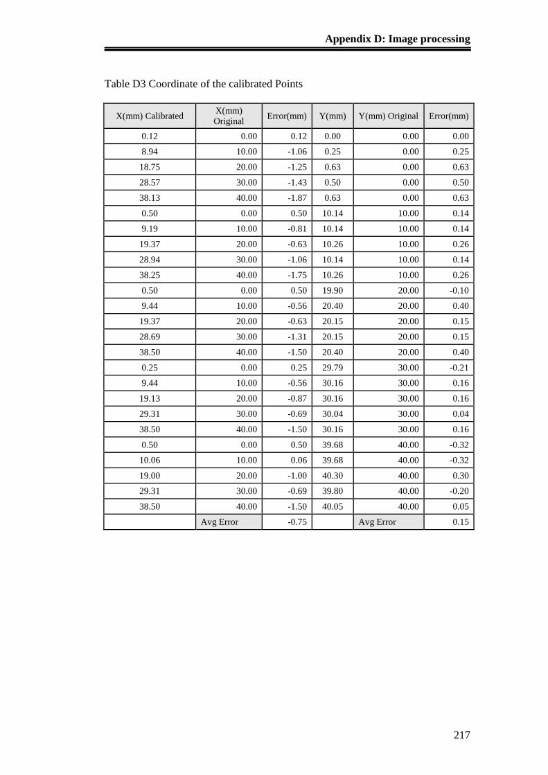
Appendix D: Image processing
217
Table D3 Coordinate of the calibrated Points
X(mm) Calibrated X(mm)
Original Error(mm) Y(mm) Y(mm) Original Error(mm)
0.12 0.00 0.12 0.00 0.00 0.00
8.94 10.00 -1.06 0.25 0.00 0.25
18.75 20.00 -1.25 0.63 0.00 0.63
28.57 30.00 -1.43 0.50 0.00 0.50
38.13 40.00 -1.87 0.63 0.00 0.63
0.50 0.00 0.50 10.14 10.00 0.14
9.19 10.00 -0.81 10.14 10.00 0.14
19.37 20.00 -0.63 10.26 10.00 0.26
28.94 30.00 -1.06 10.14 10.00 0.14
38.25 40.00 -1.75 10.26 10.00 0.26
0.50 0.00 0.50 19.90 20.00 -0.10
9.44 10.00 -0.56 20.40 20.00 0.40
19.37 20.00 -0.63 20.15 20.00 0.15
28.69 30.00 -1.31 20.15 20.00 0.15
38.50 40.00 -1.50 20.40 20.00 0.40
0.25 0.00 0.25 29.79 30.00 -0.21
9.44 10.00 -0.56 30.16 30.00 0.16
19.13 20.00 -0.87 30.16 30.00 0.16
29.31 30.00 -0.69 30.04 30.00 0.04
38.50 40.00 -1.50 30.16 30.00 0.16
0.50 0.00 0.50 39.68 40.00 -0.32
10.06 10.00 0.06 39.68 40.00 -0.32
19.00 20.00 -1.00 40.30 40.00 0.30
29.31 30.00 -0.69 39.80 40.00 -0.20
38.50 40.00 -1.50 40.05 40.00 0.05
Avg Error -0.75 Avg Error 0.15
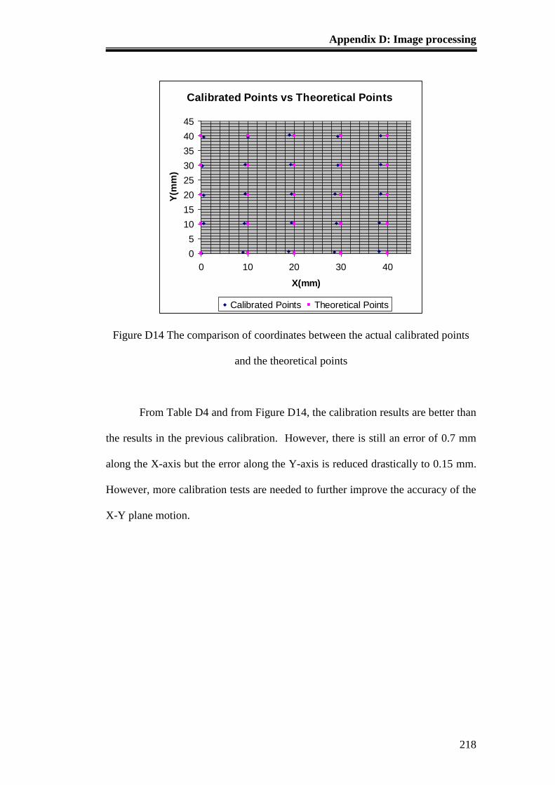
Appendix D: Image processing
218
Figure D14 The comparison of coordinates between the actual calibrated points
and the theoretical points
From Table D4 and from Figure D14, the calibration results are better than
the results in the previous calibration. However, there is still an error of 0.7 mm
along the X-axis but the error along the Y-axis is reduced drastically to 0.15 mm.
However, more calibration tests are needed to further improve the accuracy of the
X-Y plane motion.
Calibrated Points vs Theoretical Points
0
5
10
15
20
25
30
35
40
45
0 10 20 30 40
X(mm)
Y(m
m)
Calibrated Points Theoretical Points
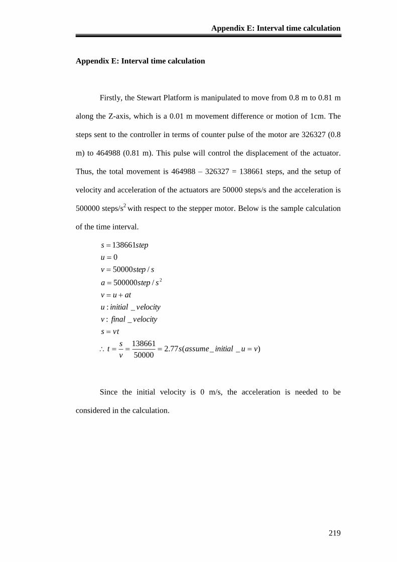
Appendix E: Interval time calculation
219
Appendix E: Interval time calculation
Firstly, the Stewart Platform is manipulated to move from 0.8 m to 0.81 m
along the Z-axis, which is a 0.01 m movement difference or motion of 1cm. The
steps sent to the controller in terms of counter pulse of the motor are 326327 (0.8
m) to 464988 (0.81 m). This pulse will control the displacement of the actuator.
Thus, the total movement is 464988 – 326327 = 138661 steps, and the setup of
velocity and acceleration of the actuators are 50000 steps/s and the acceleration is
500000 steps/s2
with respect to the stepper motor. Below is the sample calculation
of the time interval.
)__(77.250000
138661
_:
_:
/500000
/50000
0
138661
2
vuinitialassumesv
st
vts
velocityfinalv
velocityinitialu
atuv
sstepa
sstepv
u
steps
Since the initial velocity is 0 m/s, the acceleration is needed to be
considered in the calculation.
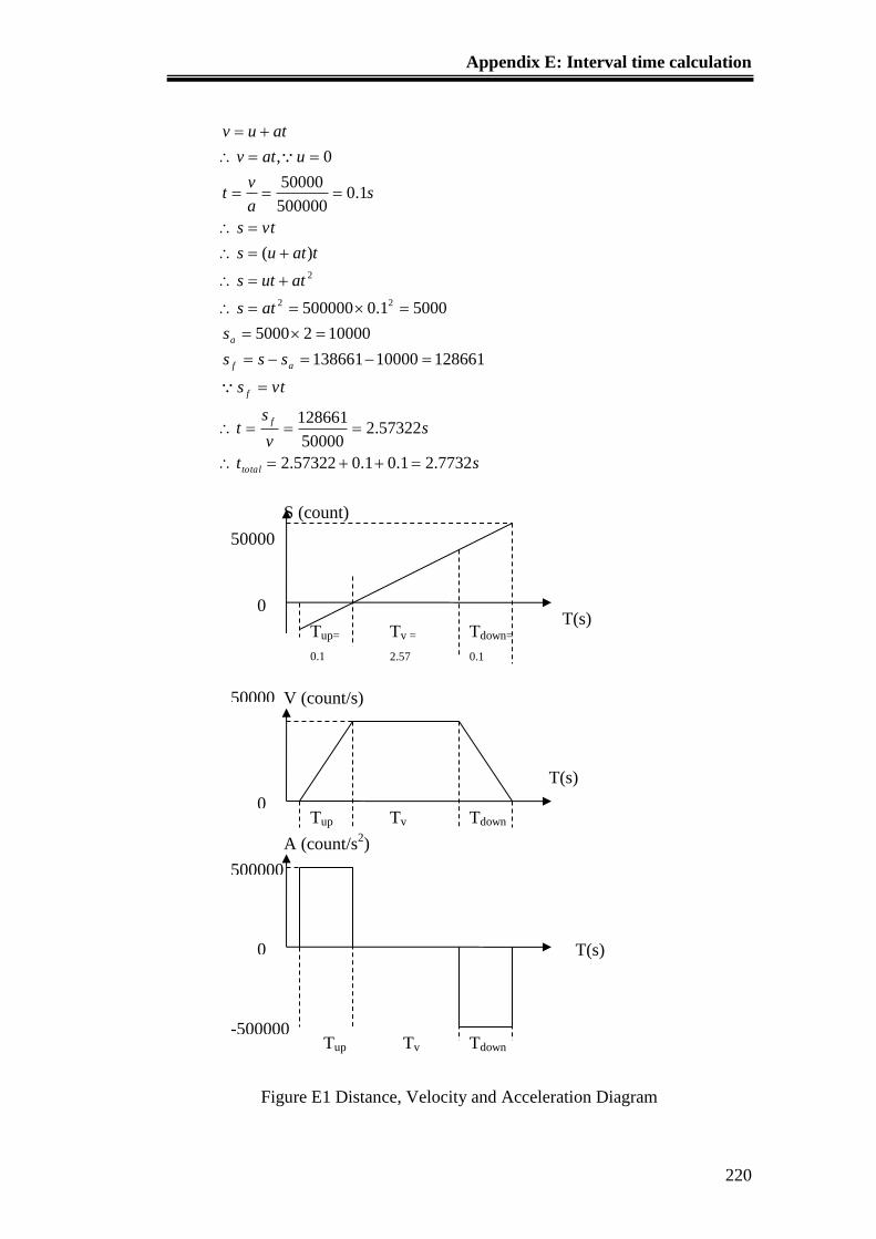
Appendix E: Interval time calculation
220
st
sv
st
vts
sss
s
ats
atuts
tatus
vts
sa
vt
uatv
atuv
total
f
f
af
a
7732.21.01.057322.2
57322.250000
128661
12866110000138661
1000025000
50001.0500000
)(
1.0500000
50000
0,
22
2
Figure E1 Distance, Velocity and Acceleration Diagram
V (count/s)
T(s)
50000
0 Tup Tv Tdown
A (count/s2)
T(s) 0
500000
0
Tup Tv Tdown
S (count)
T(s)
50000
0
Tv =
2.57
Tdown=
0.1
Tup=
0.1
-500000
Appendix E: Interval time calculation
221
Even though according to calculation, the time needed for the actuator to
move to the final destination is 2.77s but in the actual manipulation of the
platform there is a time delay due to friction and inertia.
The time interval is the key control of communication between the CPU
and the controller. There is problem of jamming of actuators during manipulation
corresponding to the trajectory path. It is because signals sent to the Stewart
Platform are sent constantly in the interval time of 100 ms. The Stewart Platform
cannot reach the destination in 100 ms before the following signal is updated to
the controller. In the long run, there are more commands accumulated in the
controller card before the actuator can execute all of them immediately. Until
certain time, the controller card will be jammed due to the overwhelming amount
of data stored. Hence a more comprehensive algorithm is needed to improve the
communication between the PC and the controller card.
Therefore, the solution is to vary the time interval with respect to the travel
distance so that when the travel distance is long, the time interval will become
longer corresponding to the travel distance. Similarly, when the travel distance is
shorter, the interval time will be shortened. Alternatively, another method is to
adjust the velocity of the respective actuator based on travel distance. When the
travel distance is very far away, the velocity will be increased so that the actuator
will move within the limitation of the travel time.
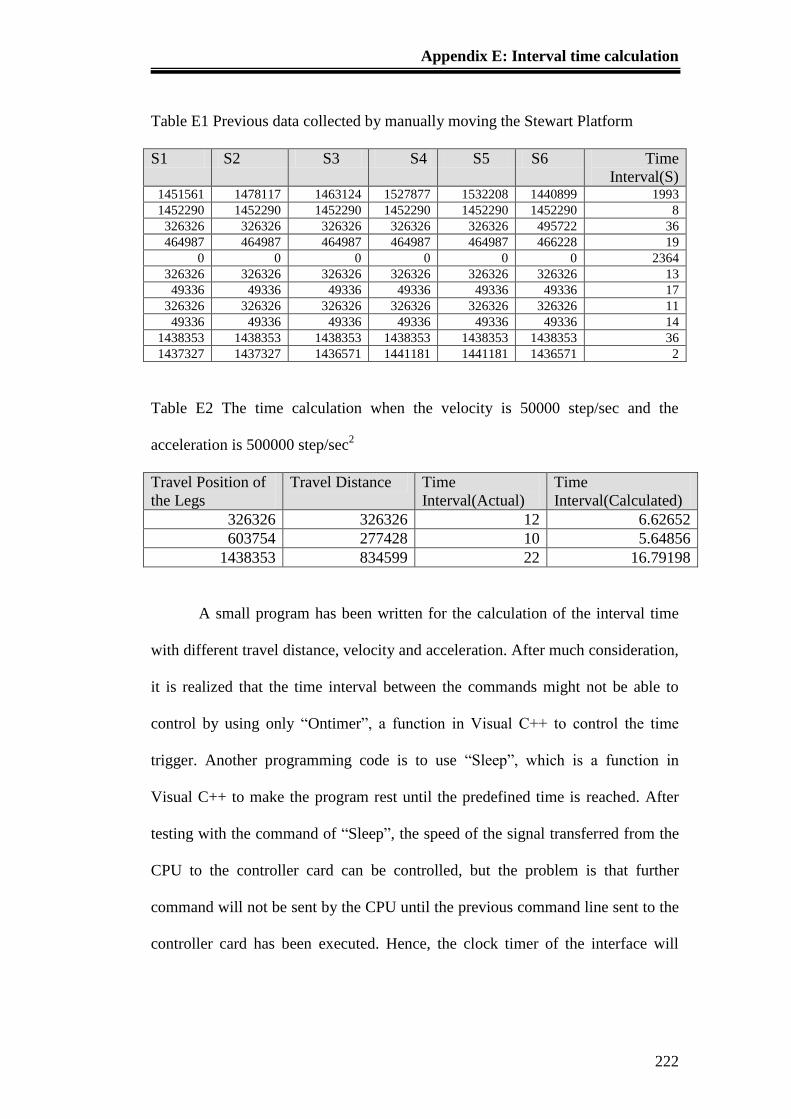
Appendix E: Interval time calculation
222
Table E1 Previous data collected by manually moving the Stewart Platform
S1 S2 S3 S4 S5 S6 Time
Interval(S) 1451561 1478117 1463124 1527877 1532208 1440899 1993
1452290 1452290 1452290 1452290 1452290 1452290 8
326326 326326 326326 326326 326326 495722 36
464987 464987 464987 464987 464987 466228 19
0 0 0 0 0 0 2364
326326 326326 326326 326326 326326 326326 13
49336 49336 49336 49336 49336 49336 17
326326 326326 326326 326326 326326 326326 11
49336 49336 49336 49336 49336 49336 14
1438353 1438353 1438353 1438353 1438353 1438353 36
1437327 1437327 1436571 1441181 1441181 1436571 2
Table E2 The time calculation when the velocity is 50000 step/sec and the
acceleration is 500000 step/sec2
Travel Position of
the Legs
Travel Distance Time
Interval(Actual)
Time
Interval(Calculated)
326326 326326 12 6.62652
603754 277428 10 5.64856
1438353 834599 22 16.79198
A small program has been written for the calculation of the interval time
with different travel distance, velocity and acceleration. After much consideration,
it is realized that the time interval between the commands might not be able to
control by using only “Ontimer”, a function in Visual C++ to control the time
trigger. Another programming code is to use “Sleep”, which is a function in
Visual C++ to make the program rest until the predefined time is reached. After
testing with the command of “Sleep”, the speed of the signal transferred from the
CPU to the controller card can be controlled, but the problem is that further
command will not be sent by the CPU until the previous command line sent to the
controller card has been executed. Hence, the clock timer of the interface will
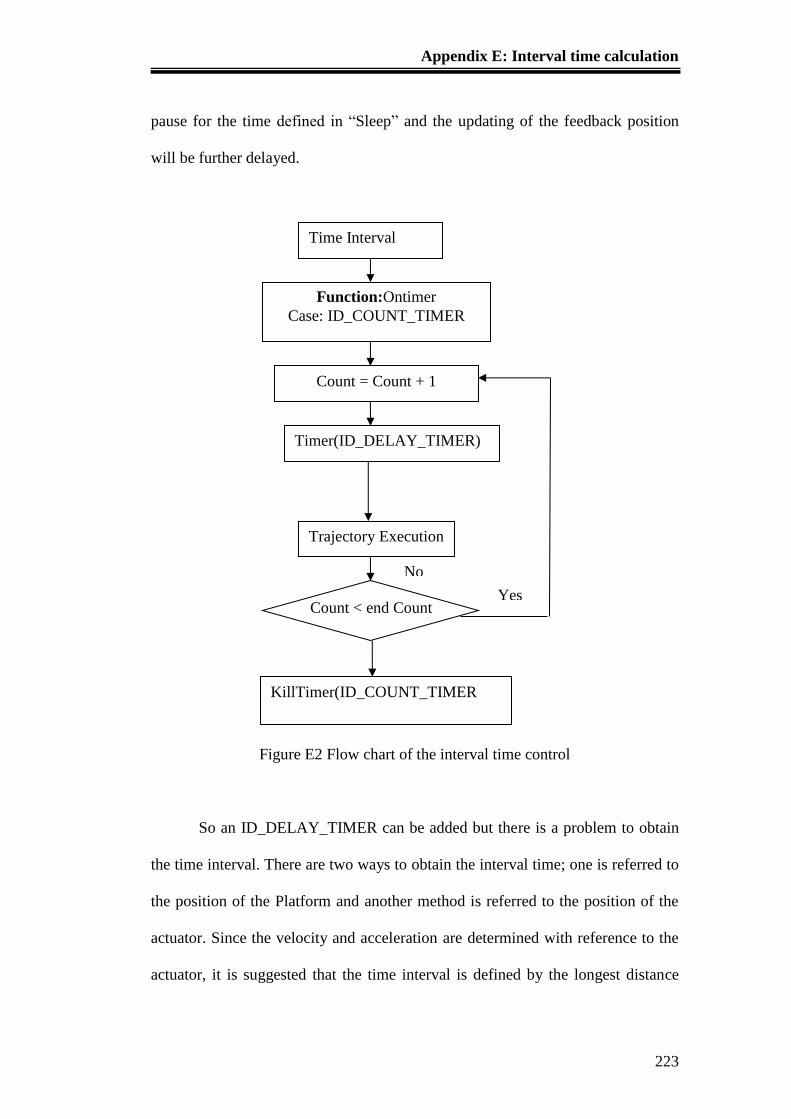
Appendix E: Interval time calculation
223
pause for the time defined in “Sleep” and the updating of the feedback position
will be further delayed.
Figure E2 Flow chart of the interval time control
So an ID_DELAY_TIMER can be added but there is a problem to obtain
the time interval. There are two ways to obtain the interval time; one is referred to
the position of the Platform and another method is referred to the position of the
actuator. Since the velocity and acceleration are determined with reference to the
actuator, it is suggested that the time interval is defined by the longest distance
Time Interval
Function:Ontimer
Case: ID_COUNT_TIMER
Count = Count + 1
Trajectory Execution
Count < end Count
KillTimer(ID_COUNT_TIMER
Yes
No
Timer(ID_DELAY_TIMER)
Appendix E: Interval time calculation
224
traveled among the six actuators. So a function must be written to decide which
one has the longest travel distance.
After the implementation of the above-mentioned method in the developed
software program of the Stewart Platform, it is proven that the previous jamming
error which is caused by the insufficient time interval can now be solved. Hence
by controlling the given time interval correctly, the Stewart Platform can now run
more than 300 lines of trajectory path command. The capability of the Stewart
Platform to execute more than 300 lines of command helps to improve the
potential of Stewart Platform to be used in machining processes.