
2. The Two-Body Problem - ULiege · 2. The Two-Body Problem 2.2 Gravitational field: 2.2.1...
105
Gaëtan Kerschen Space Structures & Systems Lab (S3L) 2. The Two-Body Problem Astrodynamics (AERO0024)
-
Upload
nguyenhanh -
Category
Documents
-
view
223 -
download
1
Transcript of 2. The Two-Body Problem - ULiege · 2. The Two-Body Problem 2.2 Gravitational field: 2.2.1...

Gaëtan Kerschen
Space Structures &
Systems Lab (S3L)
2. The Two-Body Problem
Astrodynamics (AERO0024)

2
2. The Two-Body Problem
2.3 Relative motion
2.4 Resulting orbits
3r
r r
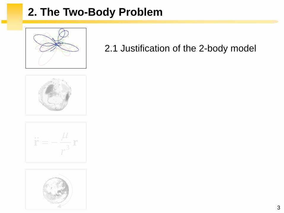
2.1 Justification of the 2-body model
X
Y
2.2 Gravitational field
3
2. The Two-Body Problem
2.1 Justification of the 2-body model
3r
r r
X
Y

5
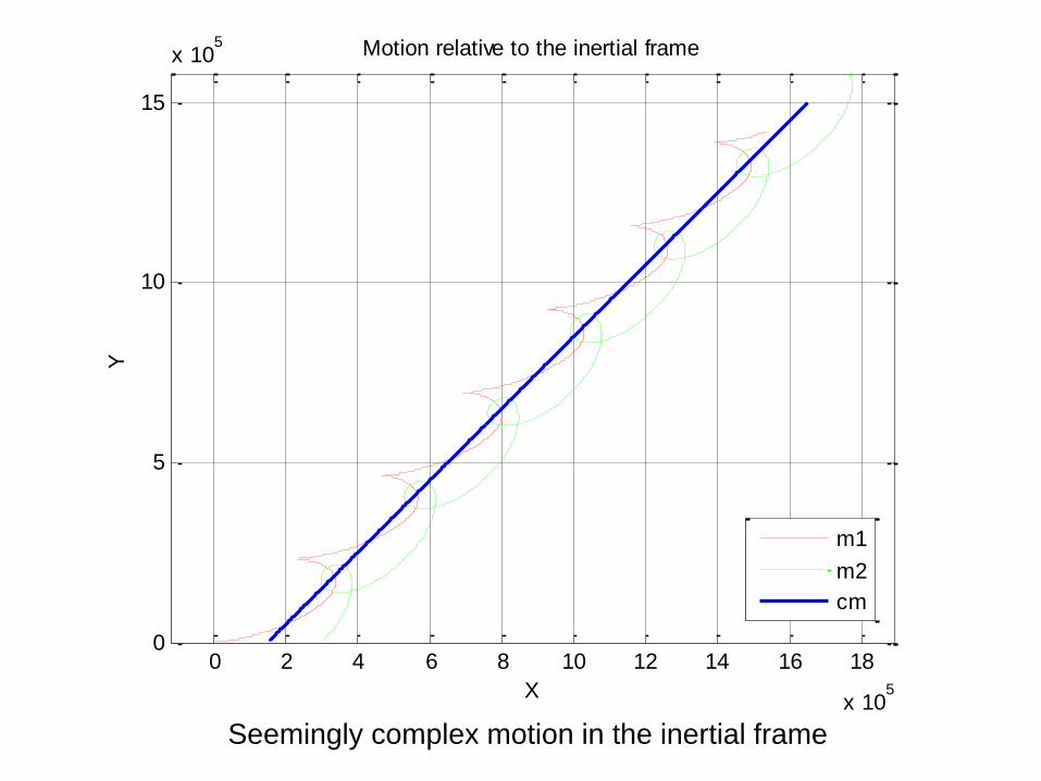
Two-Body Problem: Matlab Example
Two identical masses:
One is at rest at the origin of the inertial frame of reference.
The other one has a velocity directed upward to the right making
a 45 degrees angle with the X axis.
m1
m2
v0
X
Y
2.1 Justification of the two-body model
0 2 4 6 8 10 12 14 16 18
x 105
0
5
10
15
x 105 Motion relative to the inertial frame
X
Y
m1
m2
cm
Seemingly complex motion in the inertial frame

-1.5 -1 -0.5 0 0.5 1 1.5
x 105
-1
-0.5
0
0.5
1
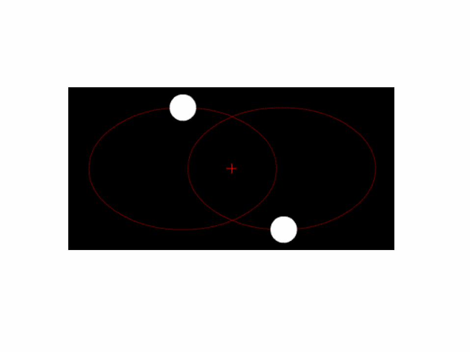
x 105 Motion relative to the center of mass
X
Y
m1
m2
Much less complex motion when
viewed from the c.o.m
0 0.5 1 1.5 2 2.5 3
x 105
-1
-0.5
0
0.5
1
1.5
x 105 Motion of m
2 relative to m
1
X
Y
Much less complex motion when
viewed from m1
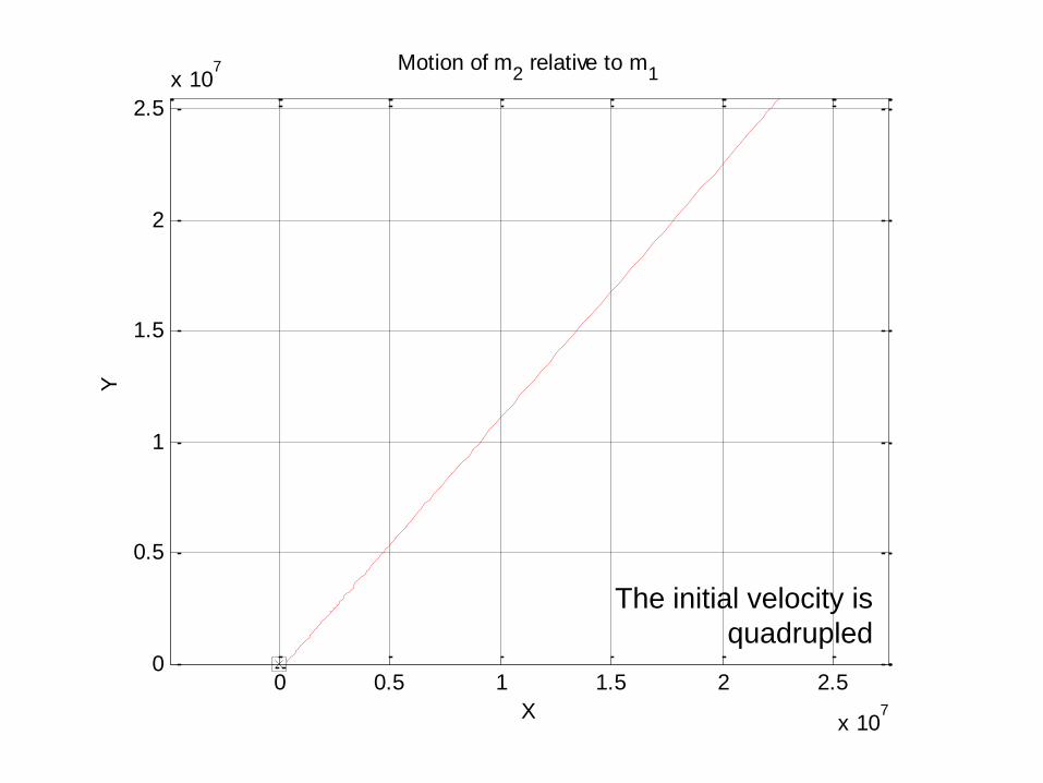
0 0.5 1 1.5 2 2.5
x 107
0
0.5
1
1.5
2
2.5
x 107 Motion of m
2 relative to m
1
X
Y
The initial velocity is
quadrupled

10
Three-Body Problem: Matlab Example
Three identical masses:
Two are at rest.
The third one has a velocity directed upward to the right making
a 45 degrees angle with the X axis.
m1
m2
v0
X
Y
m3
2.1 Justification of the two-body model
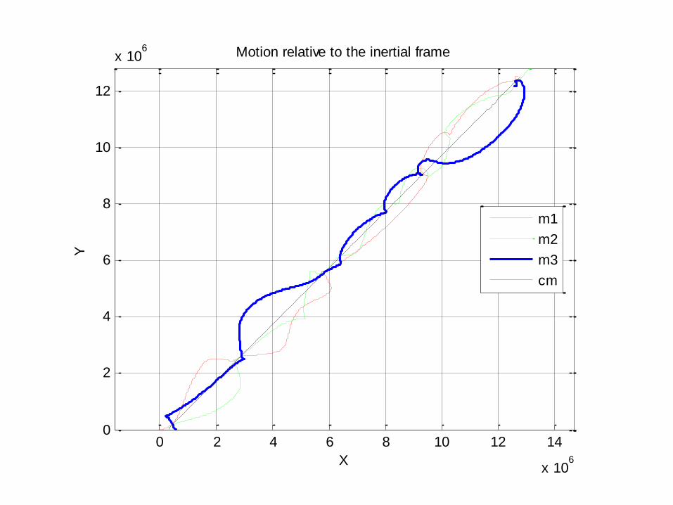
0 2 4 6 8 10 12 14
x 106
0
2
4
6
8
10
12
x 106 Motion relative to the inertial frame
X
Y
m1
m2
m3
cm

-1 -0.5 0 0.5 1
x 106
-10
-8
-6
-4
-2
0
2
4
6
8
x 105 Motion relative to the center of mass
X
Y
m1
m2
m3
What Do You Conclude ?

0 2 4 6 8 10 12 14 16 18
x 105
0
5
10
15
x 105 Motion relative to the inertial frame
X
Y
m1
m2
cm
Seemingly complex motion in the inertial frame

14
Why Is the 3-Body Problem So Difficult ?
0 0.5 1 1.5 2 2.5 3
x 104
0
2
4
6
8
10
12
14
16x 10
5 Comparison of time series
Time
Dis
pla
cem
ent
of
the f
irst
mass (
x d
irection)
Nominal IC
Perturbed IC
0 5 10 15
x 104
0
2
4
6
8
10
12
14x 10
6 Comparison of time series
Time
Dis
pla
cem
ent
of
the f
irst
mass (
x d
irection)
Nominal IC
Perturbed IC
3-body problem
(initial conditions perturbed by 0.1%)
Chaotic by nature !
2.1 Justification of the two-body model
2-body problem
(initial conditions perturbed by 0.1%)
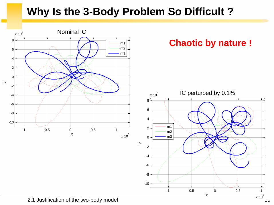
15
Why Is the 3-Body Problem So Difficult ?
-1 -0.5 0 0.5 1
x 106
-10
-8
-6
-4
-2
0
2
4
6
8
x 105 Nominal IC
X
Y
m1
m2
m3
-1 -0.5 0 0.5 1
x 106
-10
-8
-6
-4
-2
0
2
4
6
8
x 105 IC perturbed by 0.1%
X
Y
m1
m2
m3
Chaotic by nature !
2.1 Justification of the two-body model

16
Precise orbit propagation:
Elaborate models are necessary to compute the motion
of satellites to the high level of accuracy required for
many applications today (e.g., the GPS system). The 2-
body problem is not helpful in that context.
2.1 Justification of the two-body model
Interest in the Two-Body Problem ?

17 2.1 Justification of the two-body model
Interest in the Two-Body Problem ?
Qualitative understanding:
The main features of satellite and planet orbits can be
described by a reasonably simple approximation, the
two-body problem.
Interplanetary transfer:
In lecture 6, we will use a sequence of 2-body problems
to approximate a complex interplanetary mission.
Mission design:
Some important quantities (ΔV and C3) can be computed
fairly accurately using the two-body assumption.
18
2. The Two-Body Problem
2.2 Gravitational field:
2.2.1 Newton’s law of universal gravitation
2.2.2 The Earth
2.2.3 Gravity models and geoid
3r
r r What is the highest point on
Earth ?

19
Gravitational Force
The law of universal gravitation is an
empirical law describing the
gravitational attraction between bodies
with mass.
It was first formulated by Newton in
Philosophiae Naturalis Principia
Mathematica (1687). He was able to
relate objects falling on the Earth to
the motion of the planets. Isaac Newton (1642-1727)
2.2.1 Newton’s law of universal gravitation

20
Gravitational Force
Every point mass attracts every other point mass by a force
pointing along the line intersecting both points. The force is
proportional to the product of the two masses and inversely
proportional to the square of the distance between the point
masses:
2.2.1 Newton’s law of universal gravitation

21
In Vector Form
1 212 122
12
ˆm m
G F rr
2 112
2 11
12 2 1
ˆ
r rr
r r
r r r
with
2.2.1 Newton’s law of universal gravitation
22
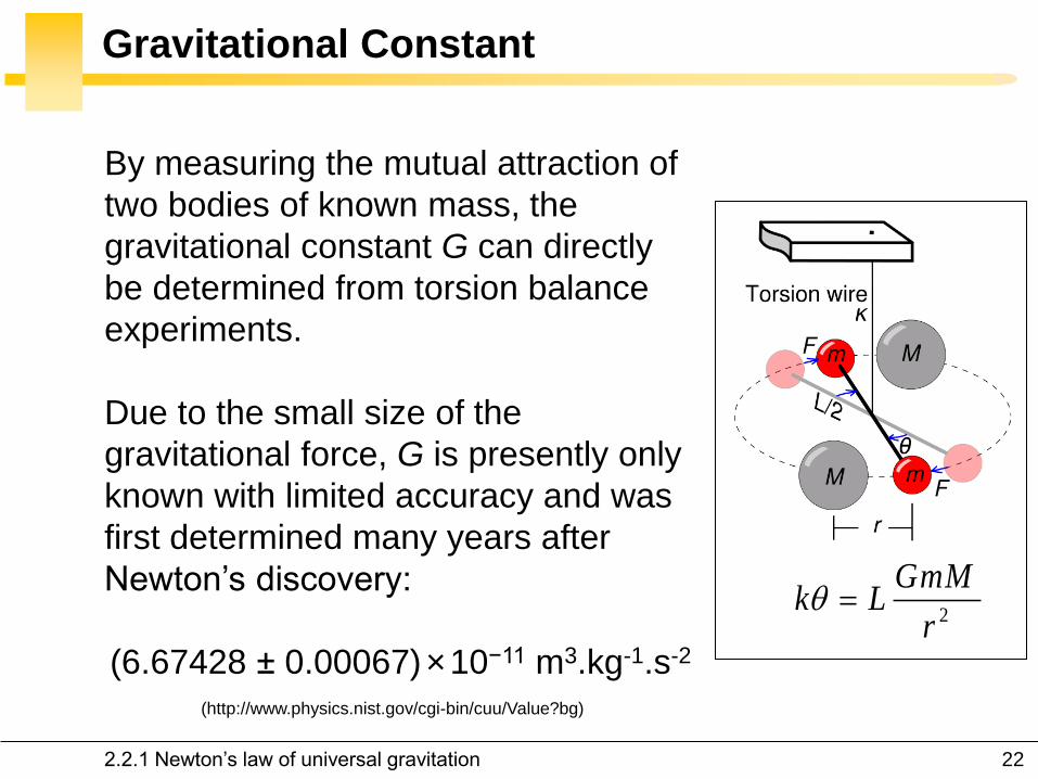
Gravitational Constant
By measuring the mutual attraction of
two bodies of known mass, the
gravitational constant G can directly
be determined from torsion balance
experiments.
Due to the small size of the
gravitational force, G is presently only
known with limited accuracy and was
first determined many years after
Newton’s discovery:
(6.67428 ± 0.00067) × 10−11 m3.kg-1.s-2
(http://www.physics.nist.gov/cgi-bin/cuu/Value?bg)
2
GmMk L
r
2.2.1 Newton’s law of universal gravitation

23
Gravitational Parameter of a Celestial Body
GM
The gravitational parameter of the Earth has been
determined with considerable precision from the analysis of
laser distance measurements of artificial satellites:
398600.4418 ± 0.0008 km3.s-2.
The uncertainty is 1 to 5e8, much smaller than the
uncertainties in G and M separately (~1 to 1e4 each).
2.2.1 Newton’s law of universal gravitation

24
Satellite Laser Ranging
2.2.1 Newton’s law of universal gravitation
Lasers measure ranges from ground stations to satellite borne retro-reflectors.
Because the events of sending and receiving a pulse can be registered within a few
picoseconds, the distance between the ground station and the satellite is determined
within a few millimeters.
LAGEOS-1 TIGO (Concepcion, Chile)

25
Acceleration of Gravity
2
GMg
r
We sense our own weight by feeling contact forces acting
on us in opposition to the force of gravity: W=mg.
If planetary gravity is the only force acting on a body, then
the body is said to be in free fall. There are, by definition, no
contact forces, so there can be no sense of weight.
A person in free fall experiences weightlessness: gravity is
still there, but he cannot feel it.
2
,
, ,
, ,
9.807 m/s
%
%
earth SL
earth aircraft earth SL
earth ISS earth SL
g
g g
g g
0.3
10
2.2.1 Newton’s law of universal gravitation
26
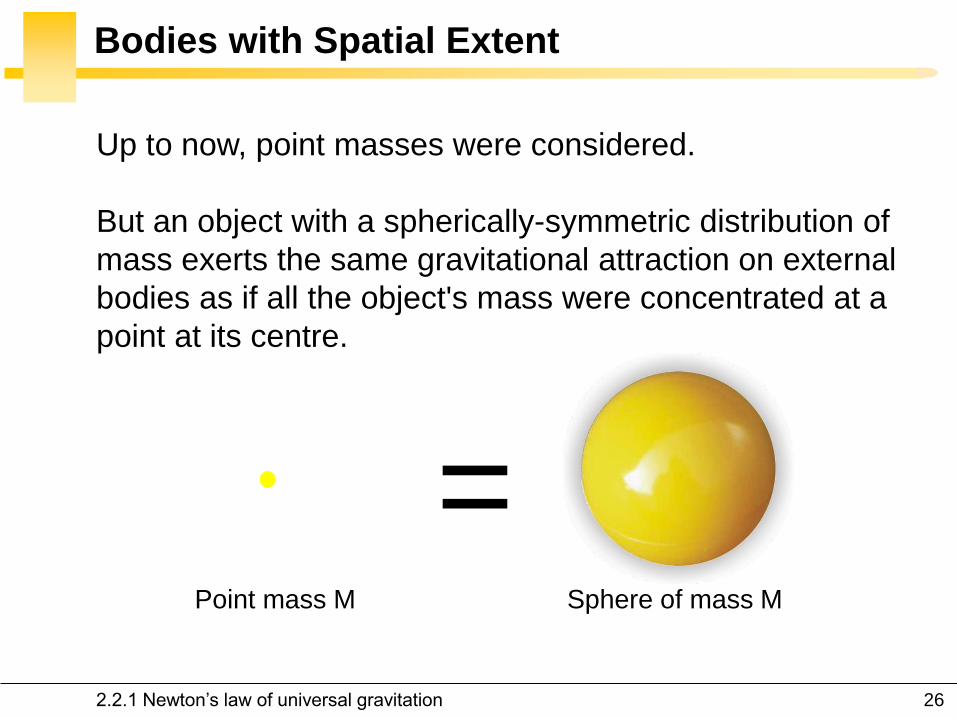
Bodies with Spatial Extent
Up to now, point masses were considered.
But an object with a spherically-symmetric distribution of
mass exerts the same gravitational attraction on external
bodies as if all the object's mass were concentrated at a
point at its centre.
Sphere of mass M Point mass M
=
2.2.1 Newton’s law of universal gravitation

27
Spherically Symmetric Mass Distribution
v
dvV Gm
r
m
( ', , )dv r
r'r
2' sin d d d 'dv r r
vM dv
2 2' 2 ' cosr R r r R
M
' sindr r R
d r
2.2.1 Newton’s law of universal gravitation

28
Spherically Symmetric Mass Distribution
0 022 2
0 0 0 0d sin d ' d ' 4 ' d '
R R
M r r r r
0
0
0
2
0 0
'2
0 '
2
0
sin d2 ' d '
1 2 d ' d '
'
4 ' d '
R
R R r
R r
R
V Gm r rr
Gm r r rr R
Gm GMmr r
R R
OK !
2.2.1 Newton’s law of universal gravitation

29
What is the Highest Point on Earth ?
Mount Chimborazo (6310 m), located in Ecuador, may be
considered as the highest point on Earth. It is the spot on
the surface farthest from the Earth’s center.
6384.4 km (Chimborazo) vs. 6382.3 km (Everest)
2.2.2 The Earth

30
The Earth is not a Sphere…
2.2.2 The Earth

31
1st Order Effect: Equatorial Bulge
Because our planet rotates, the
centrifugal force tends to pull material
outwards around the Equator where
the velocity of rotation is at its highest:
The Earth’s radius is 21km greater at
the Equator compared to the poles.
The force of gravity is weaker at the
Equator (g=9.78 m/s2) than it is at the
poles (g=9.83 m/s2).
2.2.2 The Earth

32
2nd Order Effect: Mountains and Oceans
Rather than being smooth, the surface
of the Earth is relatively “lumpy”:
There is about a 20 km difference in
height between the highest mountain
and the deepest part of the ocean
floor.
2.2.2 The Earth

33
3rd Order Effect: Internal Mass Distribution
The different materials that make up
the layers of the Earth’s crust and
mantle are far from homogeneously
distributed:
For instance, the crust beneath the
oceans is a lot thinner and denser
than the continental crust.
2.2.2 The Earth

34
The Idealized Geometrical Figure of the Earth
Because of its relative simplicity, a flattened ellipsoid, called
the reference ellipsoid, is typically used as the idealized
Earth:
Ellipsoid of revolution.
The size is represented by the radius at the equator, a.
The shape of the ellipsoid is given by the flattening, f, which
indicates how much the ellipsoid departs from spherical.
f=(a-b)/a, where b is the polar radius.
2.2.3 Gravity models and geoid

35
Most Common Reference Ellipsoid
WGS84 (World Geodetic System 1984, revised in 2004):
Origin at the center of mass of Earth.
a=6378.137 km, b=6356.752 km, f=0.335 %.
Reference system used by the GPS.
Official document on the course web site (interesting to read !).
WGS84 four defining parameters
2.2.3 Gravity models and geoid

36
WGS84 Coordinate System
2.2.3 Gravity models and geoid

37
Longitude
Point coordinates such as latitude, longitude and elevation
are defined from the reference ellipsoid.
The meridian of zero longitude is the IERS Reference
Meridian, which lies 5.31’’ east of the Greenwich Meridian.
2.2.3 Gravity models and geoid

38
GPS Receiver at the Greenwich Meridian
2.2.3 Gravity models and geoid
5.31/3600=0.0015
OK !

39
Latitude
Also called
geodetic latitude
2.2.3 Gravity models and geoid

40
The True Figure of the Earth
The geoid is that equipotential surface which would
coincide exactly with the mean ocean surface of the Earth,
if the oceans were in equilibrium, at rest, and extended
through the continents:
It is by definition a surface to which the force of gravity is
everywhere perpendicular.
It is an irregular surface but considerably smoother than Earth's
physical surface. While the latter has excursions of almost
20 km, the total variation in the geoid is less than 200 m.
2.2.3 Gravity models and geoid

41
The True Figure of the Earth
2.2.3 Gravity models and geoid

42
Gravitational Modeling
Spherical harmonics are used to model the Earth
gravitational model:
The current set is EGM2008 (Earth Gravity Model 2008). The
model comprises 4.6 million terms in the spherical expansion
(order and degree 2159).
Geoid with a resolution approaching 10 km (5’x5’).
More details in Chapter 4 (Non-Keplerian motion).
Gravitational potential function
2.2.3 Gravity models and geoid

43
EGM2008 Made Use of Grace Satellites
2.2.3 Gravity models and geoid
GRACE employs microwave ranging
system to measure changes in the
distance between two identical
satellites as they circle Earth. The
ranging system detects changes as
small as 10 microns over a distance
of 220 km.

44
Geoid Definition
EGM2008 contains no explicit information about which level
surface, out of the infinitely many that may be generated
from the potential coefficients, is "the" geoid.
EGM2008 model is therefore used to compute geoid
undulations with respect to WGS84 ellipsoid. The result is
referred to as WGS84-EGM08 geoid.
Geoid calculator for EGM96:
http://earth-info.nga.mil/GandG/wgs84/gravitymod/egm96/intpt.html
2.2.3 Gravity models and geoid

1: ocean
2:
3: local plumb
4: continent
5: reference ellipsoid
geoid

47
GPS Receivers
You are on a boat in the middle of the Atlantic ocean, what
will be the height indicated by your GPS ?
You are at “sea level”, but the height will be
different from 0. The GPS satellites can only
measure heights relative to the WGS84 model,
which is an idealized figure of the Earth.
2.2.3 Gravity models and geoid

48
GPS Receivers
Some GPS receivers can obtain the geoid height over the
WGS ellipsoid from the current position. They are then able
to correct the height above WGS ellipsoid to the height
above the geoid.
You are on a boat in the middle of the Atlantic ocean, will
the height indicated by this GPS be equal to zero ?
Not necessarily, because there are tides…
2.2.3 Gravity models and geoid

49
Residual Sea Surface Slopes (EGM-96)
2.2.3 Gravity models and geoid

50
Residual Sea Surface Slopes (EGM-2008)
2.2.3 Gravity models and geoid
51
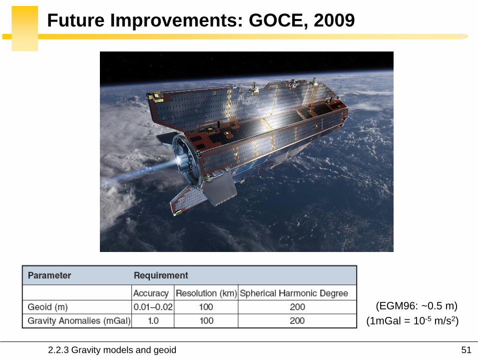
Future Improvements: GOCE, 2009
(1mGal = 10-5 m/s2)
(EGM96: ~0.5 m)
2.2.3 Gravity models and geoid

52
Why So Many Efforts ???
1. GPS and an advanced map of the geoid can replace
time-consuming leveling procedures.
2. Physics of the Earth’s interior (gravity is directly linked to
the distribution of mass).
3. Understanding of ocean circulation, which plays a key
role in energy exchanges around the globe.
4. Computation of the motion of satellites to the level of
accuracy required today.
2.2.3 Gravity models and geoid

53
Further Reading on the Course Web Site
2.2.3 Gravity models and geoid

54
Digression: General Relativity
Einstein's theory is the current description of gravity in
modern physics.
This course will not cover the theory of general relativity, but
Newton's law is still an excellent approximation of the
effects of gravity if:
2
2 21, and 1
GM v
c rc c
2.2.3 Gravity models and geoid

55
General Relativity: Earth-Sun Example
22
8 8
2 2
2~ 10 , and ~ 10
1 year.
sun orbit
orbit
GM rv
c r c c c
G=6.67428 × 10⁻¹¹ m3.kg-1.s-2
rorbit=1.5 × 10¹¹ m (1 AU)
Msun=1.9891 × 1030 kg
c=3e8 m.s-1
OK !
2.2.3 Gravity models and geoid

56
The Quest of a Unifying Theory
What is the relationship between the gravitational force
and other known fundamental forces ?
That one body may act upon another at a distance
through a vacuum without the mediation of anything else,
by and through which their action and force may be
conveyed from one another, is to me so great an
absurdity that, I believe, no man who has in philosophic
matters a competent faculty of thinking could ever fall
into it. (Newton, 1692)
The question is not yet fully resolved today !
2.2.3 Gravity models and geoid

57
The Quest of a Unifying Theory
[End of digression]
2.2.3 Gravity models and geoid

58
2. The Two-Body Problem
2.3 Relative motion:
2.3.1 Equations of motion
2.3.2 Closed-form solution
3r
r r

59
Motion of two bodies due solely to their own mutual
gravitational attraction. Also known as Kepler problem.
Assumption: two point masses (or equivalently spherically
symmetric objects).
Definition of the 2-Body Problem
?
?
2.3.1 Equations of motion
60
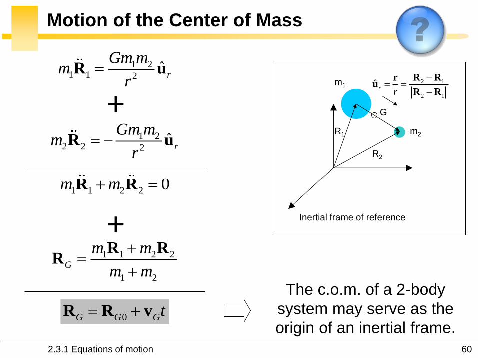
Motion of the Center of Mass
G
m2
m1
Inertial frame of reference
R1
R2
2 1
2 1
ˆr
r
R Rru
R R
1 22 2 2
ˆr
Gm mm
r R u
1 21 1 2
ˆr
Gm mm
rR u
+
1 1 2 2 0m m R R
1 1 2 2
1 2
G
m m
m m
R RR
+
0G G Gt R R v
The c.o.m. of a 2-body
system may serve as the
origin of an inertial frame.
2.3.1 Equations of motion

61
Equations of Relative Motion
G
m2
m1
Inertial frame of reference
R1
R2
2 1
2 1
ˆr
r
R Rru
R R
2
1 21 2 2 2
ˆr
Gm mm m
r R u
2
1 21 2 1 2
ˆr
Gm mm m
r
R u
+
1 2
2 1 2ˆ
r
G m m
r
R R u
3r
r r
μ is the gravitational
parameter
The motion of m2 as seen
from m1 is the same as the
motion of m1 as seen from m2.
2.3.1 Equations of motion

62
Equations of Relative Motion
3r
r r
This is a nonlinear dynamical system.
How to solve it ?
Find constants of the motion !
How many ?
2.3.2 Closed-form solution

63
Constant Angular Momentum
3r
r r
30
r
r r r r
0 constant=d
dt
hr r h
r
h r rd
dt
hr r r r r r
Specific angular
momentum
/d dt
2.3.2 Closed-form solution

64
The Motion Lies in a Fixed Plane
r
r
r
r
ˆh
h
h
ˆh
h
h
constant= r r h
The fixed plane is the
orbit plane and is normal
to the angular momentum
vector.
2.3.2 Closed-form solution

65
Azimuth Component of the Velocity
ˆˆ ˆ ˆ( )r r rr v v rv h r r u u u h
2h rv r
r r
rv
v
The angular momentum depends only on the
azimuth component of the relative velocity
2.3.2 Closed-form solution

66
First Integral of Motion
3r
r r 3 3r r
r h r h r r r
3 2. .
r d
r r r dt r
r r rr h r r r r r r
. . a b c b a c c a b2
d r r
dt r r
r r r
e lies in the orbit plane
(e.h)=0: the line defined by e
is the apse line.
Its norm, e, is the eccentricity.
h
constant=r
r
r h e
2.3.2 Closed-form solution

67
Οrbit Equation
r
r h re
. ..
r
r r h r rr e
. . a b c a b c
2. . ..
hr
r r h r r h h hr e
.r
Closed form of the nonlinear
equations of motion
2 1
1 cos
hr
e
2.3.2 Closed-form solution

68
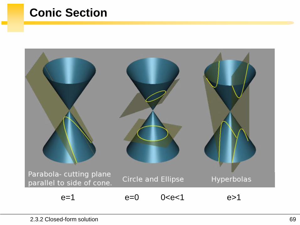
Conic Section in Polar Coordinates
2 1
1 cos 1 cos
h pr
e e
Independent variable: true
anomaly (=0 at the periapsis)
Constant: eccentricity
Constant: angular
momentum
Constant: gravitational
parameter
Semi-latus rectum
2.3.2 Closed-form solution
69
Conic Section
e=0 e=1 0<e<1 e>1
2.3.2 Closed-form solution

70
In Summary
+ We can calculate r for all values of the true anomaly.
The orbit equation is a mathematical statement of Kepler’s first law. +
Do we have 6 independent constants ?
The solution of the “simple” problem of two bodies cannot be
expressed in a closed form, explicit function of time. -
We only know the relative motion (however, e.g., the motion of our
sun relative to other parts of our galaxy is of little importance for
missions within our solar system). -
The two vector constants h and e provide
only 5 independent constants: h.e=0
2.3.2 Closed-form solution
71
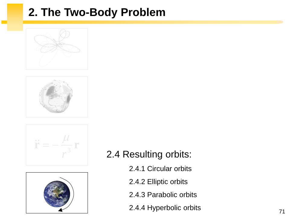
2. The Two-Body Problem
2.4 Resulting orbits:
2.4.1 Circular orbits
2.4.2 Elliptic orbits
2.4.3 Parabolic orbits
2.4.4 Hyperbolic orbits
3r
r r

72
Three Objectives
1. Period
2. Velocity
3. Energy

73
Digression: Energy of the Orbit
2
2
mv mT V
r
2
constant2
v
r
Specific energy
The gravitational force
is conservative

74
Energy of the Orbit at Periapsis
2 2 2
22 2 2
p
p
p p p p
v v h
r r r r
2 2
0
1
1 cos (1 )p
h hr
e e
2
2
2
11
2e
h
[End of digression]

75
Possible Motions in the 2-Body System
ellipse
circle
parabola hyperbola
76
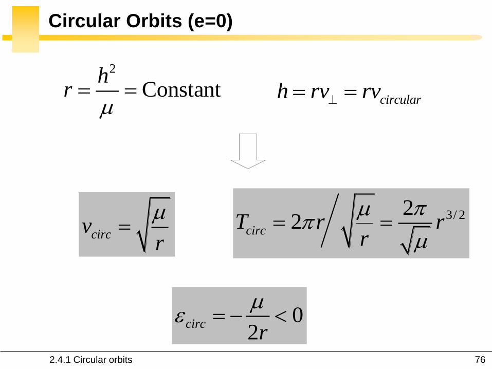
Circular Orbits (e=0)
2
Constanth
r
circularh rv rv
circvr
3/ 222circT r r
r
02
circr
2.4.1 Circular orbits

77
Orbital Speed
0 200 400 600 800 10007.3
7.4
7.5
7.6
7.7
7.8
7.9
8
Altitude (km)
Orb
ita
l sp
ee
d (
km
/s)
ISS
HST
SPOT-5
( )satG m M G M
2.4.1 Circular orbits

78
0 200 400 600 800 100080
85
90
95
100
105
110
Altitude (km)
Orb
ita
l p
eri
od
(m
in)
Orbital Period
ISS
HST
SPOT-5
2.4.1 Circular orbits

79
Hubble Space Telescope
2.4.1 Circular orbits

80
Hubble Space Telescope
2.4.1 Circular orbits

81
Two Particular Cases
1. 7.9 km/s is the first cosmic velocity; i.e., the minimum
velocity (theoretical velocity, r = 6378 km) to orbit the
Earth.
2. 35786 km is the altitude of the geostationary orbit.
* A sidereal day, 23h56m4s, is the time it takes the Earth to complete one rotation relative to inertial space. A
synodic day, 24h, is the time it takes the sun to apparently rotate once around the earth. They would be
identical if the earth stood still in space.
It is
the orbit at which the satellite angular velocity is equal to
that of the Earth, ω=ωE=7.292 10-5 rad/s, in inertial
space (*). 2/3
2
circ
GEO
Tr

82
Elliptic Orbits (0<e<1)
θ=0, minimum separation, periapse
θ=π, greatest separation, apoapse
θ=π/2, semi-latus rectum p
2 1
1 cos
hr
e
2
(1 )p
hr
e
2
(1 )a
hr
e
The relative position vector
remains bounded.
a p
a p
r re
r r
2.4.2 Elliptic orbits

83
Geometry of the Elliptic Orbit
rp ra
a
b
p
θ
apse line
2.4.2 Elliptic orbits

84
Angular Momentum and Energy
2 1
1 cos
hr
e
Orbit equation
2(1 )
1 cos
a er
e
Polar equation of an ellipse
(a, semimajor axis)
2(1 )h a e
02
ellipa
2
2
2
11
2e
h
Independent of
eccentricity !
2.4.2 Elliptic orbits

85
Vis-Viva Equation
2
2 2
v
r a
2 1ellipv
r a
2.4.2 Elliptic orbits

86
Kepler’s Second Law
1 1 1
2 2 2dA dt dt hdt r r h
21constant
2 2
dA h dr
dt dt
The line from the sun to a
planet sweeps out equal
areas inside the ellipse in
equal lengths of time.
( )tr
( )t dtr
dtr
1
2Area AB AC
reminder
2.4.2 Elliptic orbits
87
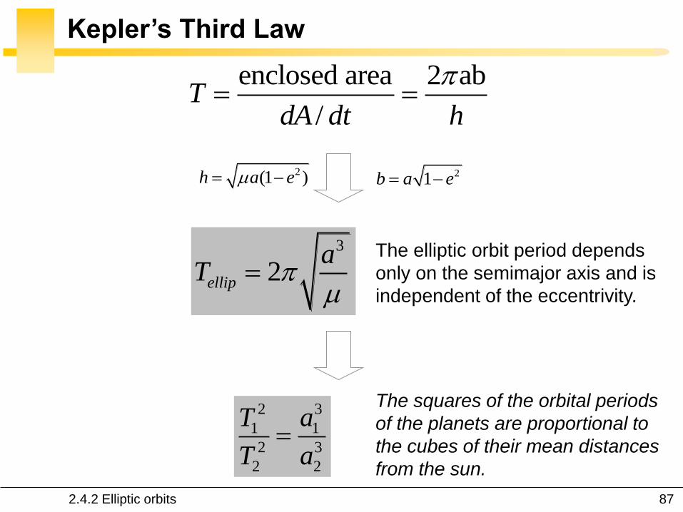
Kepler’s Third Law
enclosed area 2 ab
/T
dA dt h
2(1 )h a e 21b a e
3
2ellip
aT
The elliptic orbit period depends
only on the semimajor axis and is
independent of the eccentrivity.
The squares of the orbital periods
of the planets are proportional to
the cubes of their mean distances
from the sun.
2 3
1 1
2 3
2 2
T a
T a
2.4.2 Elliptic orbits

88
Satellite in Elliptic Orbit
354 6378 6732kmpr 1447 6378 7825kmar
0.075, 7278.5km2
a p a p
a p
r r r re a
r r
3
2 6179.79s 103mina
T
2 1v
r a
7.98km/spv
6.86km/sav
2.4.2 Elliptic orbits

89
Satellite in Elliptic Orbit
2.4.2 Elliptic orbits
90
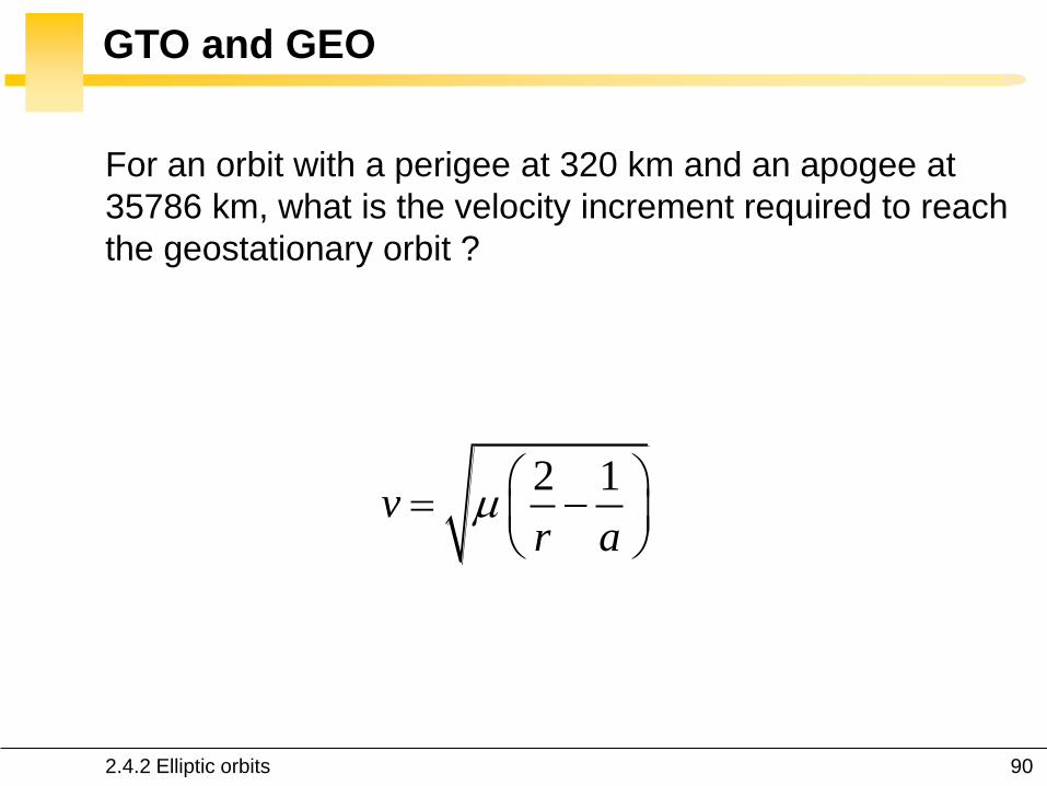
GTO and GEO
For an orbit with a perigee at 320 km and an apogee at
35786 km, what is the velocity increment required to reach
the geostationary orbit ?
2 1v
r a
2.4.2 Elliptic orbits

91
GTO and GEO
For an orbit with a perigee at 320 km and an apogee at
35786 km, what is the velocity increment required to reach
the geostationary orbit ?
24430km
2
a pr ra
10.13km/spv
1.61km/sav
GTO GEO
398000
35786 6378
3.07km/s
circv
Answer: 1.46 km/s
(apogee motor)
2.4.2 Elliptic orbits

92
GTO and GEO
100
101
102
103
104
10-4
10-3
10-2
10-1
100
v (m/s)
m
/m
Isp=300s
(1000,0.288) (1460,0.391)

93
Parabolic Orbits (e=1)
2 1
1 cos
hr
, r
2
2
v
r
2parabv
r
The satellite will coast to
infinity, arriving there with
zero velocity relative to the
central body.
2
2
2
11 0
2parab e
h
The satellite has just enough
energy to escape from the
attracting body.
2.4.3 Parabolic orbits

94
Escape Velocity, Vesc
11.2 km/s is the second cosmic velocity; i.e., the minimum
velocity (theoretical velocity, r = 6378km) to orbit the Earth.
circvr
2parabv
r
11.2km/s 2 7.9km/s
2.4.3 Parabolic orbits

95
Hyperbolic Orbits (e>1)
2 1
1 cos
hr
e
2
(1 )p
hr
e
2
0(1 )
a
hr
e
2 a pa r r
rp 2a
ra
2
2
1
1
ha
e
0
2hyper
a
2
2
2
11
2e
h
2.4.4 Hyperbolic orbits

96
C3 Velocity
2
2 2
v
a r
v
a
2 2
2 2
v v
r
2 2 2 2
3esc escv v v C v
C3 is a measure of the energy for an
interplanetary mission:
16.6 km2/s2 (Cassini-Huygens)
8.9 km2/s2 (Solar Orbiter, phase A)
Hyperbolic
excess speed
2.4.4 Hyperbolic orbits

97
Soyuz ST v2-1b (Kourou Launch)
2.4.4 Hyperbolic orbits

98
Delta II, Delta III and Atlas IIIA
2.4.4 Hyperbolic orbits

99
Proton
2.4.4 Hyperbolic orbits

100
Falcon 9
2.4.4 Hyperbolic orbits

101
The Two-Body Problem
2.1 JUSTIFICATION OF THE 2-BODY MODEL
2.2 GRAVITATIONAL FIELD
2.2.1 Newton’s law of universal gravitation
2.2.2 The Earth
2.2.3 Gravity models and geoid
2.3 RELATIVE MOTION
2.3.1 Equations of motion
2.3.2 Closed-form solution
2.4 RESULTING ORBITS
2.4.1 Circular orbits
2.4.2 Elliptic orbits
2.4.3 Parabolic orbits
2.4.4. Hyperbolic orbits

Newton’s laws
1 2
2ˆ
g r
m
m mG
r
F a
F u3r
r r
Relative motion Energy conserv.
2 1
1 cos
hr
e
2
2
v
r
Kepler’s 1st law
Angular mom.
h r r
Azim. velocity
/v h r
Kepler’s 2nd law
/ / 2dA dt h
The orbit
equation
Kepler’s 3rd law
1.5 0.52 /T a

103
Concluding Remarks
Closed-form solution from which we deduced Kepler’s laws.
Analytic formulas for orbital energy, velocity and period.
Two-body propagator available in STK. Often used in early
studies to perform trending analysis.
But …
We have lost track of the time variable !

104
Did you Know ?
Compactness of the solar system: measured by the ratio of
the distance a of a planet from the Sun to the radius R of
the Sun.
Compactness of the hydrogen atom: measured by the ratio
of the distance a of an electron from the nucleus to the
radius R of the nucleus.
200a
R
5 4a
eR

Gaëtan Kerschen
Space Structures &
Systems Lab (S3L)
2. The Two-Body Problem
Astrodynamics (AERO0024)