LIOUVILLE'S EQUATION AND THE n-BODY PROBLEM

1

LIOUVILLE'S EQUATION AND THE n-BODY PROBLEM

by R. GI Lungeburtel

Goddard Spuce Flight Center Greenbelt, M d .

NATIONAL AERONAUTICS AND SPACE ADMINISTRATION WASHINGTON, D. C. APRIL 1965

1

TECH LIBRARY KAFB, NM

00b79b3

NASA TR R-217


By R. G. Langebartel

Goddard Space Flight Center Greenbelt, Md.

NATIONAL AERONAUTICS AND SPACE ADMINISTRATION

For sale by the Office of Technical Services, Department of Commerce,

Washington, D.C. 20230 -- Price 43.00

LIOUVILLE’S EQUATION AND THE n-BODY PROBLEM

by R. G . Langebartel

Goddard Space Flight Center

SUMMARY

The motion of a system of particles is examined on the basis of the fundamental equation in statistical mechanics. The Dirac delta function is used to describe systems which are discrete in position space, velocity space, o r both as degenerate cases of continuous systems. The approximation procedure, necessitated by the nonlinearity of the problems, is based on the use of expansions in successive derivatives of the delta function. This approach leads to sum-difference-differential equations of a novel form for the quantities of interest, equations subject to a variety of techniques for solution. The method is applied to the dispensing and dispersion of the “West Ford Needles” belt, and to the problem of permanence of symmetry of the configuration of a collection of Echo-type satellites.

iii

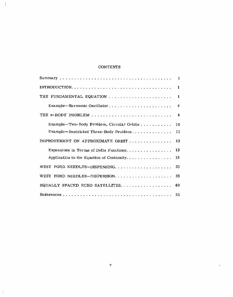
CONTENTS

Summary . . . . . . . . . . . . . . . . . . . . . . . . . . . . . . . . . . . . . . . i

INTRODUCTION . . . . . . . . . . . . . . . . . . . . . . . . . . . . . . . . . . . 1

THE FUNDAMENTAL EQUATION . . . . . . . . . . . . . . . . . . . . . . 1

Example-Harmonic Oscillator . . . . . . . . . . . . . . . . . . . . . . 4

THE n-BODY PROBLEM . . . . . . . . . . . . . . . . . . . . . . . . . . . . 4

Example-Two-Body Problem. Circular Orbits . . . . . . . . . . . 10

Example-Restricted Three-Body Problem . . . . . . . . . . . . . . 11

IMPROVEMENT ON APPROXIMATE ORBIT . . . . . . . . . . . . . . . 12

Expansions in Terms of Delta Functions . . . . . . . . . . . . . . . . 12 Application to the Equation of Continuity . . . . . . . . . . . . . . . . 16

WEST FORD NEEDLES-DISPENSING . . . . . . . . . . . . . . . . . . . . 25

WEST FORD NEEDLES-DISPERSION . . . . . . . . . . . . . . . . . . . . 35

EQUALLY SPACED ECHO SATELLITES . . . . . . . . . . . . . . . . . . 40

References . . . . . . . . . . . . . . . . . . . . . . . . . . . . . . . . . . . . . . 55

V


bY R. G. Langebartel

Goddard Space Flight Center

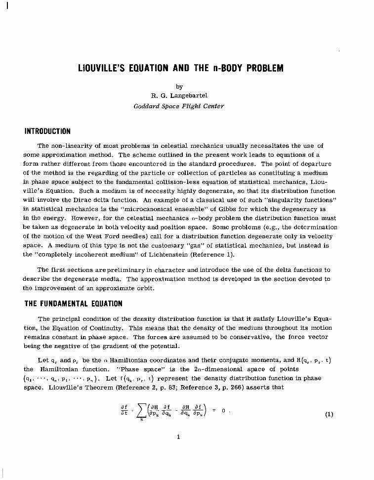
INTRODUCTION

The non-linearity of most problems in celestial mechanics usually necessitates the use of some approximation method. The scheme outlined in the present work leads to equations of a form rather different from those encountered in the standard procedures. The point of departure of the method is the regarding of the particle or collection of particles as constituting a medium in phase space subject to the fundamental collision-less equation of statistical mechanics, Liou- ville's Equation. Such a medium is of necessity highly degenerate, so that its distribution function will involve the Dirac delta function. An example of a classical use of such "singularity functions" in statistical mechanics is the T'microcanonical ensemble" of Gibbs for which the degeneracy is in the energy. However, for the celestial mechanics n-body problem the distribution function must be taken as degenerate in both velocity and position space. Some problems (e.g., the determination of the motion of the West Ford needles) call for a distribution function degenerate only in velocity space. A medium of this type is not the customary "gas" of statistical mechanics, but instead is the "completely incoherent medium" of Lichtenstein (Reference 1).

The first sections are preliminary in character and introduce the use of the delta functions to describe the degenerate media. The approximation method is developed in the section devoted to the improvement of an approximate orbit.

THE FUNDAMENTAL EQUATION

The principal condition of the density distribution function is that it satisfy Liouville's Equa- tion, the Equation of Continuity. This means that the density of the medium throughout its motion remains constant in phase space. The forces are assumed to be conservative, the force vector being the negative of the gradient of the potential.

Let q, and p, be the n Hamiltonian coordinates and their conjugate momenta, and H (qr , p , , t )

the Hamiltonian function. "Phase space" is the 2n-dimensional space of points (ql, ... , q n I p l , - , p, ) . Let f (qk, p r , t) represent the density distribution function in phase space. Liouville's Theorem (Reference 2, p. 83; Reference 3, p. 266) asserts that

1

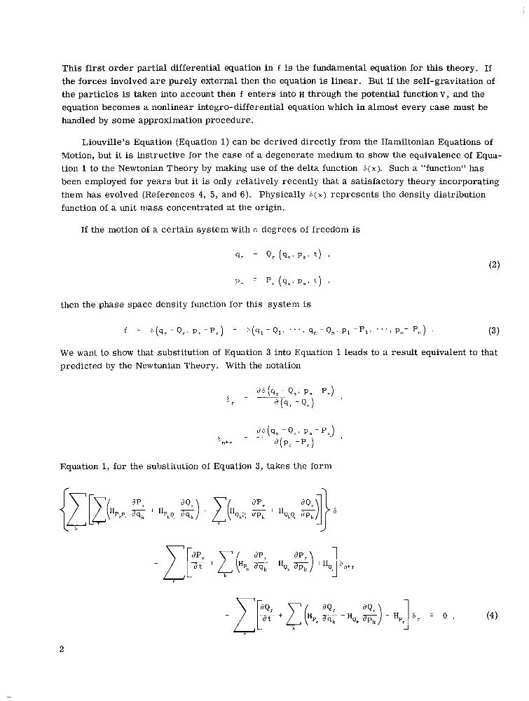
This first order partial differential equation in f is the fundamental equation for this theory. If the forces involved are purely external then the equation is linear. But if the self-gravitation of the particles is taken into account then f enters into H through the potential function v , and the equation becomes a nonlinear integro-differential equation which in almost every case must be handled by some approximation procedure.

Liouville's Equation (Equation 1) can be derived directly from the Hamiltonian Equations of Motion, but it is instructive for the case of a degenerate medium to show the equivalence of Equa- tion l to the Newtonian Theory by making use of the delta function S(x). Such a "function" has been employed for years but it is only relatively recently that a satisfactory theory incorporating them has evolved (References 4, 5, and 6). Physically &(x) represents the density distribution function of a unit mass concentrated at the origin.

If the motion of a certain system with n degrees of freedom is

9, = Q, ( q s 9 p S , t ) , (2 )

P, = pr (q., P * - t ) 3

then the phase space density function for this system is

f = b ( q r - Q r , p , - P , ) E b ( q l - Q l , . . . 7 qn - Q n x P I - P I , . * - , pn- P n ) . (3 1

We want to show that substitution of Equation 3 into Equation 1 leads to a result equivalent to that predicted by the Newtonian Theory. With the notation

Equation 1, for the substitution of Equation 3, takes the form

2

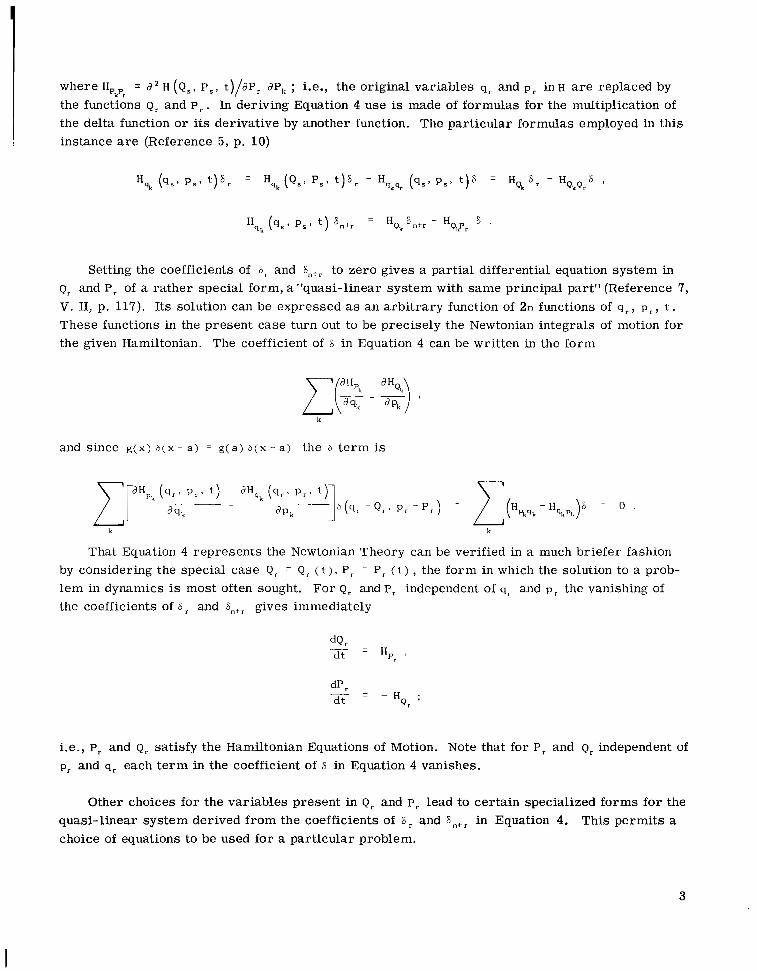
where H,, d Z H (Qs, P, , t ) / d P , d P , ; i.e., the original variables qr and p, in H are replaced by the functions Q, and P, . In deriving Equation 4 use is made of formulas for the multiplication of the delta function or its derivative by another function. The particular formulas employed in this instance are (Reference 5, p. 10)

k r

Setting the coefficients of S r and S n t r to zero gives a partial differential equation system in Q, and Pr of a rather special form, a "quasi-linear system with same principal part" (Reference 7, V. 11, p. 117). Its solution can be expressed as an arbitrary function of 2n functions of q r , p , , t . These functions in the present case turn out to be precisely the Newtonian integrals of motion for the given Hamiltonian. The coefficient of b in Equation 4 can be written in the form

and since g ( x ) b ( x - a ) = g( a ) b ( x - a) the b term is

That Equation 4 represents the Newtonian Theory can be verified in a much briefer fashion by considering the special case Q, Q, ( t ) , P r = Pr ( t ) , the form in which the solution to a problem in dynamics is most often sought. For Q, and p, independent of q r and p , the vanishing of the coefficients of S r and S n t r gives immediately

i.e., P, and Q, satisfy the Hamiltonian Equations of Motion. Note that for P r and Q, independent of p, and q, each term in the coefficient of 6 in Equation 4 vanishes.

Other choices for the variables present in Q, and P, lead to certain specialized forms for the quasi-linear system derived from the coefficients of 6 r and 6,+, in Equation 4. This permits a choice of equations to be used for a particular problem.

3

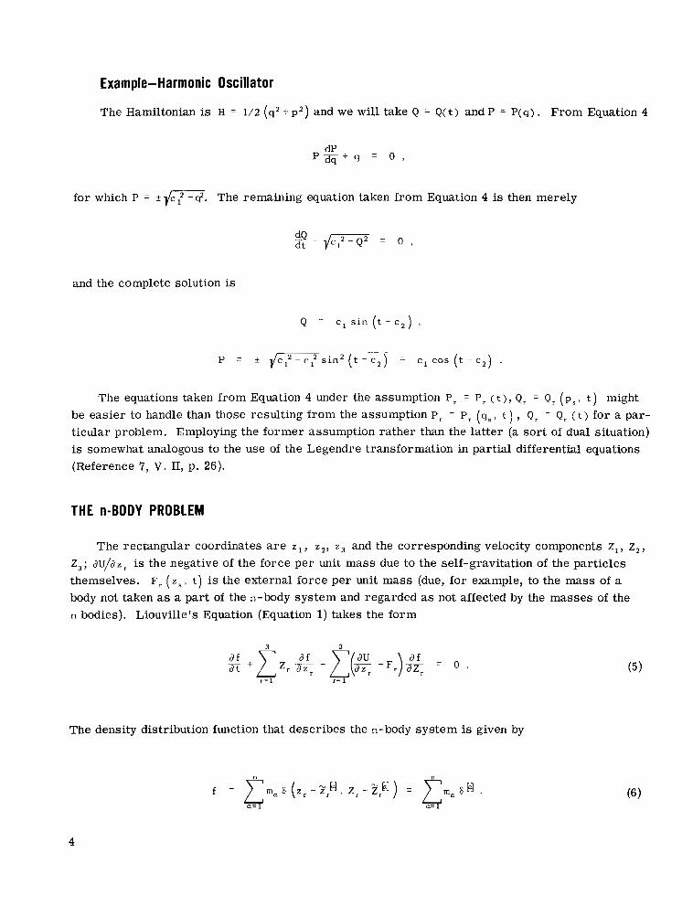
Example-Harmonic Oscillator

The Hamiltonian is H = 1/2 (qz + p 2 ) and we will take Q = Q( t ) and P = P(q) . From Equation 4

P * + q = 0 I

dP

for which P = ? ic3. The remaining equation taken from Equation 4 is then merely

and the complete solution is

Q = c1 s i n ( t -c,) ,

The equations taken from Equation 4 under the assumption Pr = Pr ( t ) , Q, = Q, ( p , , t ) might be easier to handle than those resulting from the assumption P, = P, (q., t ) , Q, = Q, ( t ) for a particular problem. Employing the former assumption rather than the latter (a sor t of dual situation) is somewhat analogous to the use of the Legendre transformation in partial differential equations (Reference 7, V. 11, p. 26).

THE n-BODY PROBLEM

The rectangular coordinates are z l , z,, z3 and the corresponding velocity components z,, z,, Z,; a u / a ~ , is the negative of the force per unit mass due to the self-gravitation of the particles themselves. F, ( z S , t ) is the external force per unit mass (due, for example, to the mass of a body not taken as a part of the n-body system and regarded as not affected by the masses of the n bodies). Liouville’s Equation (Equation 1) takes the form

The density distribution function that describes the n-body system is given by

4

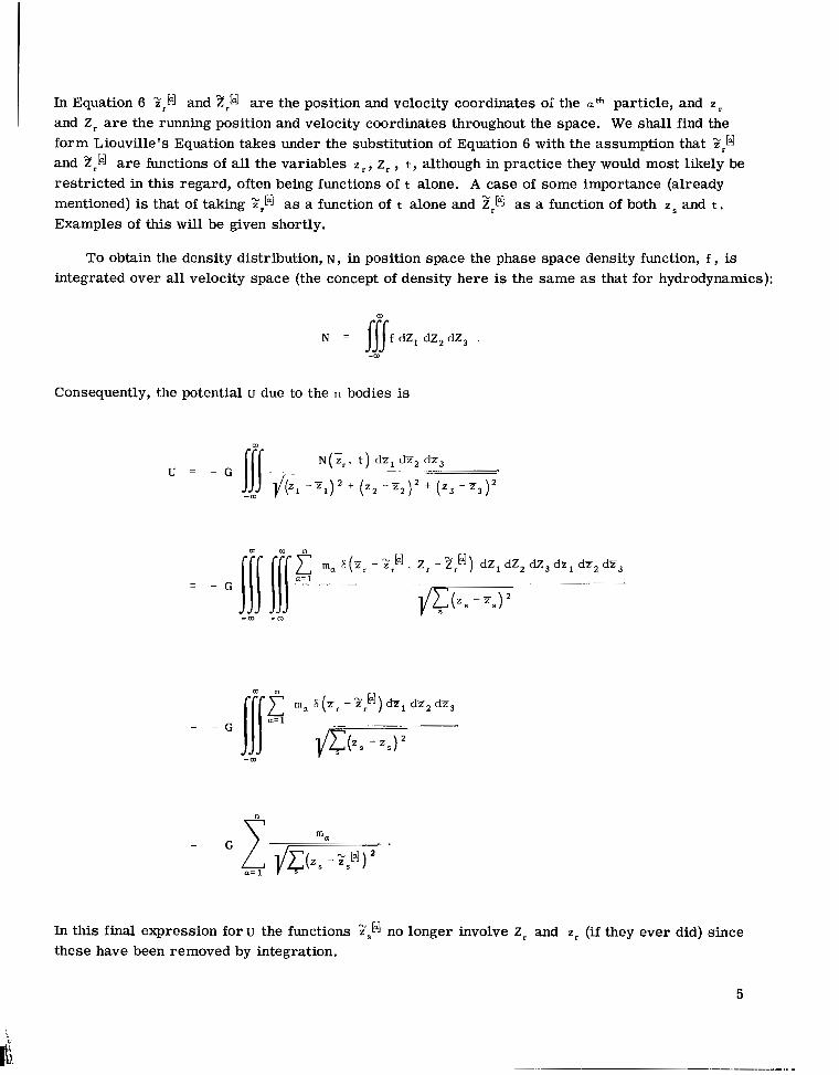
In Equation 6 ;r[d and zr[d are the position and velocity coordinates oi the uth particle, and zr and Z, are the running position and velocity coordinates throughout the space. We shall find the form Liouville's Equation takes under the substitution of Equation 6 with the assumption that ;r[d

and zrM are functions of all the variables z,, z, , t , although in practice they would most likely be restricted in this regard, often being functions of t alone. A case of some importance (already mentioned) is that of taking ?,[a3 as a function of t alone and zrM as a function of both z S and t . Examples of this will be given shortly.

To obtain the density distribution, N, in position space the phase space density function, f , is integrated over all velocity space (the concept of density here is the same as that for hydrodynamics):

N = JJJf dZ, dZ, dZ, . -m

Consequently, the potential u due to the n bodies is

= - I//- - ..

N ( X , , t ) dz, dz, dz, " i(zl - F l y t (z, -z,y t (z, - z 3 y

~~

-m

In this f i n a l expression for u the functions zsH no longer involve Zr and Z, (if they ever did) since these have been removed by integration.

5

i

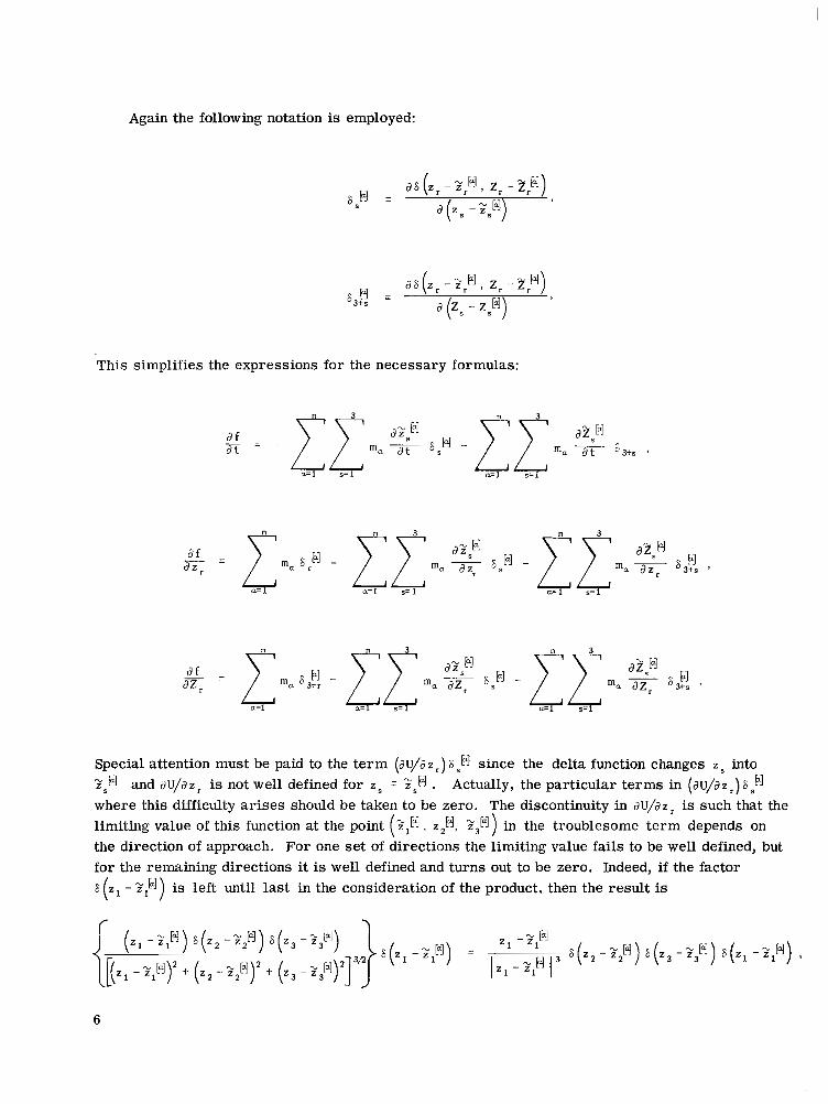
Again the following notation is employed:

This simplifies the expressions for the necessary formulas:

Special attention must be paid to the term (dU/dz,) 8,pl since the delta function changes z 5 into 2sH and dU/dz is not well defined for zS = ;sH . Actually, the particular terms in (du/bz =) 6 where this difficulty ar ises should be taken to be zero. The discontinuity in dU/dz, is such that the limiting value of this function at the point (;,["I z2[al, Z3H) in the troublesome term depends on the direction of approach. For one set of directions the limiting value fails to be well defined, but for the remaining directions it is well defined and turns out to be zero. Indeed, if the factor 6 (z l - Zlb]) is left until last in the consideration of the product. then the result is

6

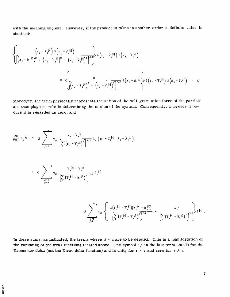
with the meaning unclear. However, if the product is taken in another order a definite value is obtained:

il (. - 2p) 6 (z - 21[d) 6 ( z* -z2[d) s ( z 3 - 1 3 q

[(zl - r 1 q z + ( z 2 f (z3 -zp)2]

Moreover, the term physically represents the action of the self-gravitation force of the particle and thus plays no role in determining the motion of the system. Consequently, wherever it oc- curs it is regarded as zero, and

In these sums, as indicated, the terms where p = u are to be deleted. This is a manifestation of the vanishing of the weak functions treated above. The symbol 6 yS in the last term stands for the Kronecker delta (not the Dirac delta function) and is unity for r = s and zero for r # s.

7

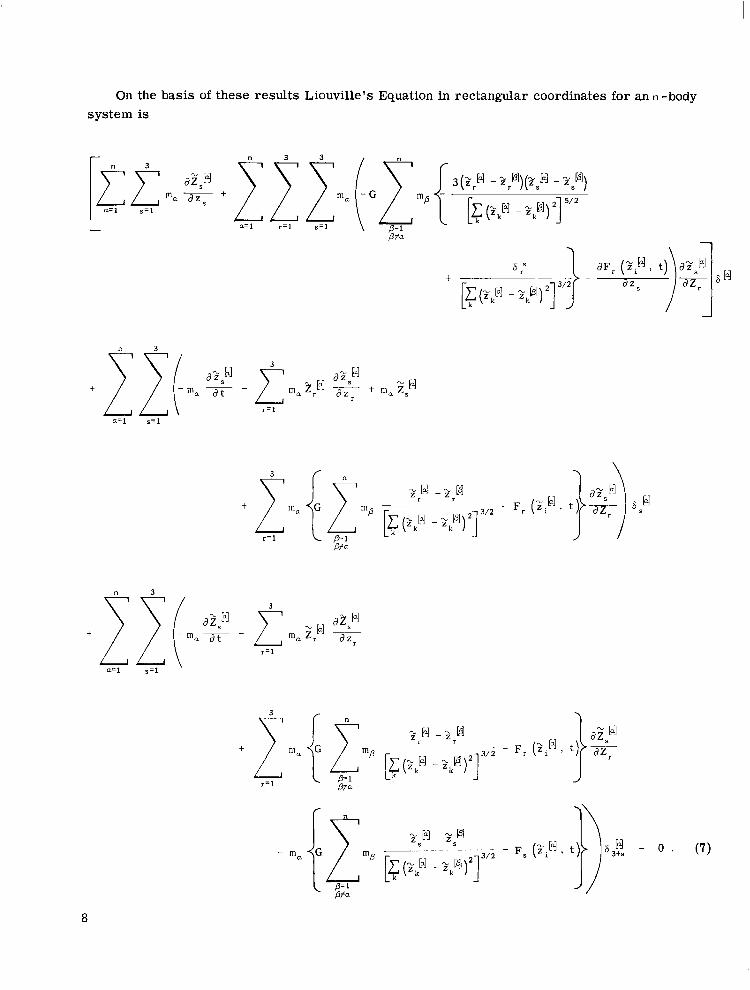
On the basis of these results Liouville's Equation in rectangular coordinates for an n -body system is

'I

8

I

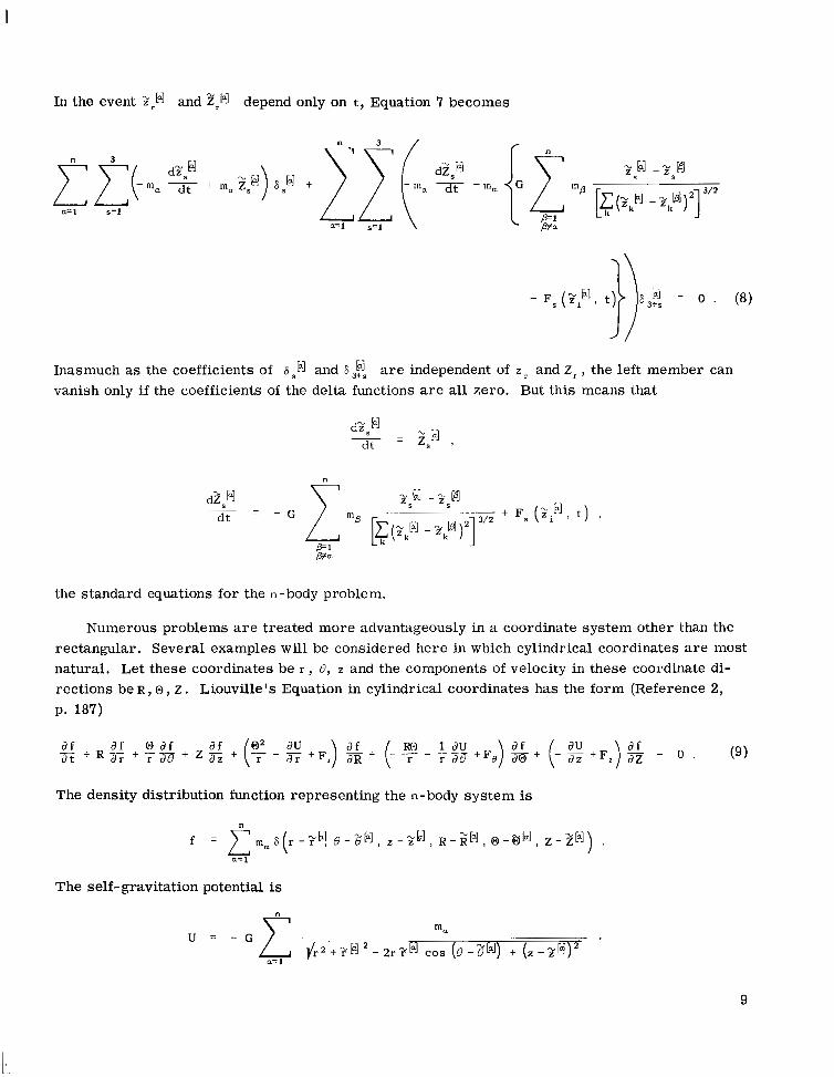
In the event yrH and zrH depend only on t, Equation 7 becomes

a=l s = I

ma (. [E p k P 1 - y,[61)2] 3'2 k

Inasmuch as the coefficients of S s b ] and 8 2 ; a r e independent of z r and Z r , the left member can vanish only i f the coefficients of the delta functions a r e all zero. But this means that

the standard equations for the n-body problem.

Numerous problems are treated more advantageously in a coordinate system other than the rectangular. Several examples will be considered here in which cylindrical coordinates are most natural. Let these coordinates be r , 8 , z and the components of velocity in these coordinate directions be R , 0, z . Liouville's Equation in cylindrical coordinates has the form (Reference 2, p. 187)

The density distribution function representing the n-body system is

a= 1

The self-gravitation potential is

9

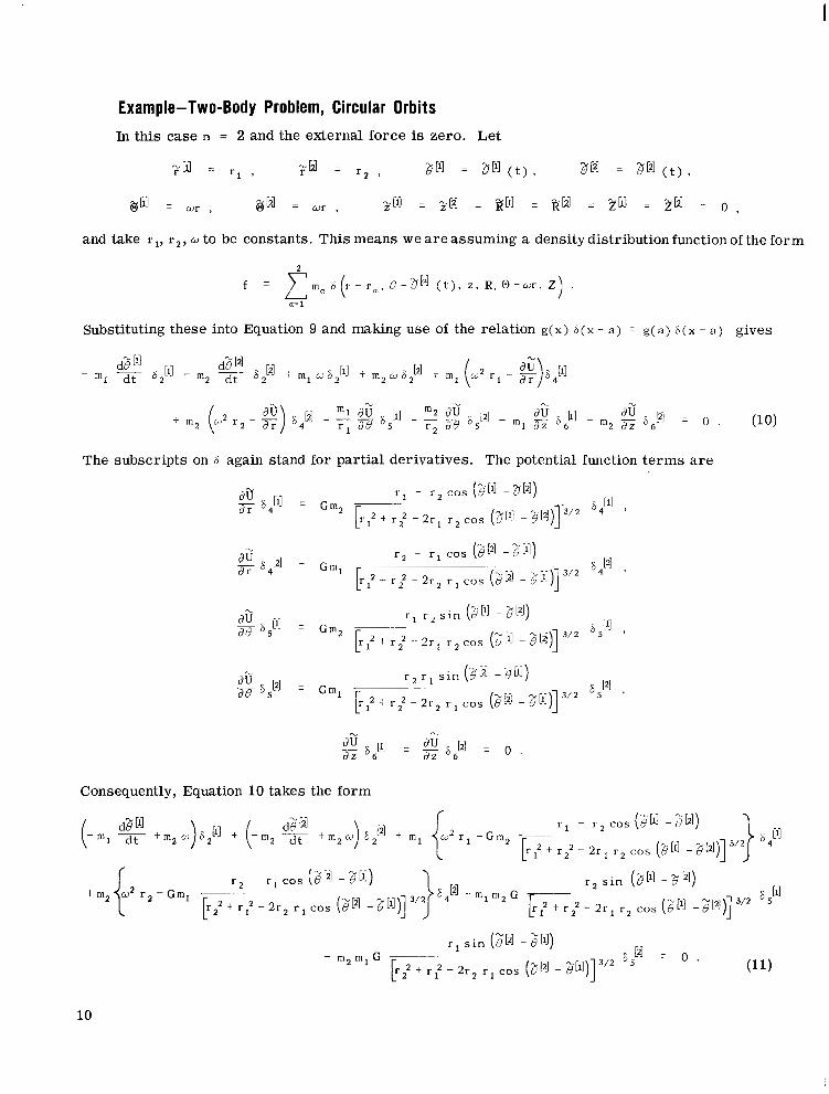
and take r l y r 2 ) w to be constants. This means we areassuming a densitydistributionfunction of the form

a= 1

Substituting these into Equation 9 and making use of the relation g( X ) &(X - a) = g( a ) S ( X - a ) gives

The subscripts on 6 again stand for partial derivatives. The potential function terms are

Consequently, Equation 10 takes the form

10

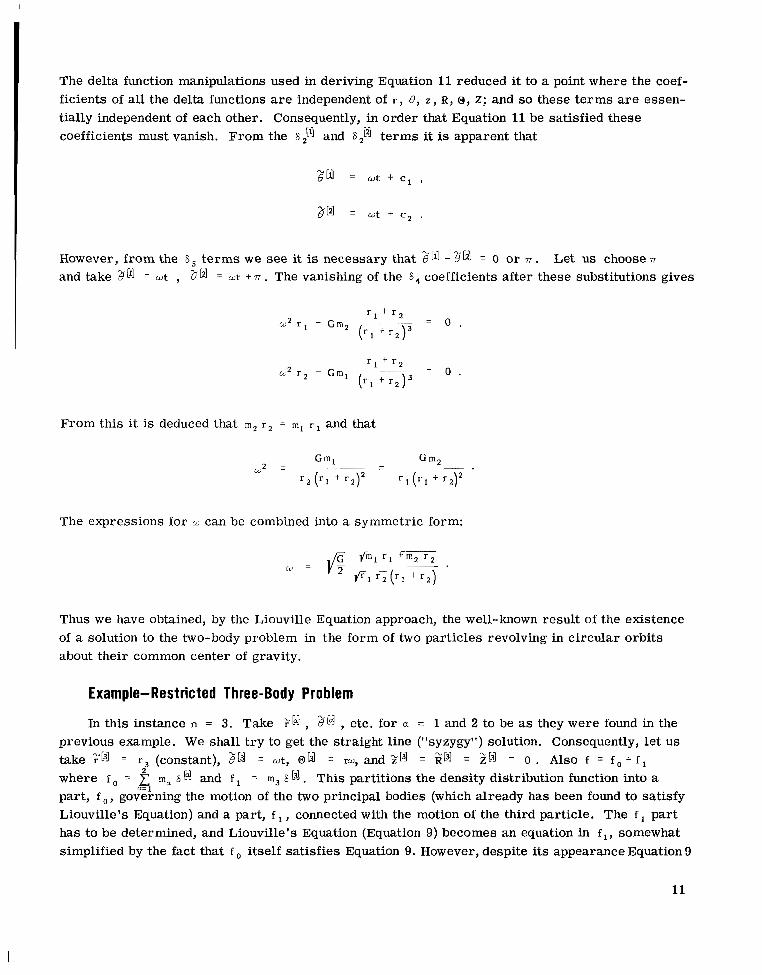
The delta function manipulations used in deriving Equation 11 reduced it to a point where the coefficients of all the delta functions are independent of r , 8, Z , R , 0, z; and so these terms are essen- t ially independent of each other. Consequently, in order that Equation 11 be satisfied these coefficients must vanish. From the 6 $1 and 6 terms it is apparent that

However, from the 6, terms we see it is necessary that %[l] - z[2J = 0 or T . Let us choose T

and take = w t , = ut + T . The vanishing of the 6, coefficients after these substitutions gives

From this it is deduced that m 2 r 2 = m l r and that

The expressions for 0: can be combined into a symmetric form:

Thus we have obtained, by the Liouville Equation approach, the well-known result of the existence of a solution to the two-body problem in the form of two particles revolving in circular orbits about their common center of gravity.

Example-Restricted Three-Body Problem

In this instance n = 3. Take "i] , 8[4 , etc. for G = 1 and 2 to be as they were found in the previous example. We shall t ry to get the straight line ("syzygy") solution. Consequently, let us take :L3] = r 3 (constant), [d = ut, 0 b] = IW, and 219 = %["I = 2 = 0 . Also f = f + f

where f = e ma 8 @ and f = m3 6 L3]. This partitions the density distribution function into a part, f o, goGegning the motion of the two principal bodies (which already has been found to satisfy Liouville's Equation) and a part, f , connected with the motion of the third particle. The f part has to be determined, and Liouville's Equation (Equation 9) becomes an equation in f l , somewhat simplified by the fact that f itself satisfies Equation 9. However, despite its appearance Equation 9

m

11

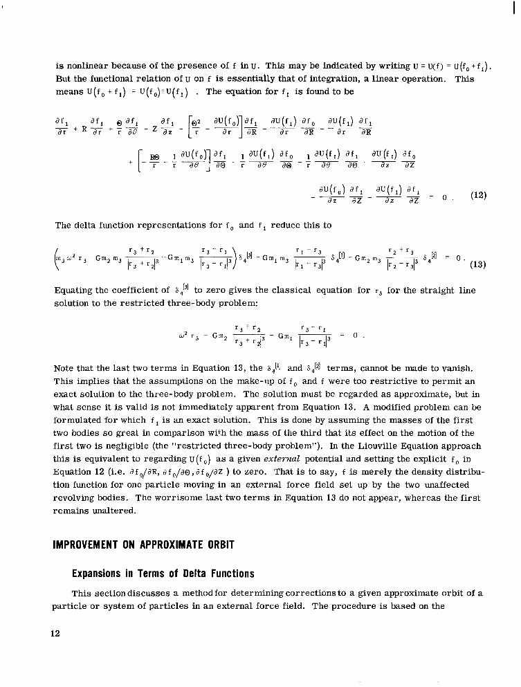
is nonlinear because of the presence of f in u. This may be indicated by writing u = u ( f ) = u ( f , + f ,) . But the functional relation of u on f is essentially that of integration, a linear operation. This means U ( f , + f , ) = U ( f , ) + U ( f , ) . The equation for f , is found to be

The delta function representations for f , and f , reduce this to

d f , d U ( f , ) d f , d Z d z d Z = . ”” (12)

Equating the coefficient of to zero gives the classical equation for r3 for the straight line solution to the restricted three-body problem:

Note that the last two terms in Equation 13, the S4[’] and S,[,] terms, cannot be made to vanish. This implies that the assumptions on the make-up of f , and f were too restrictive to permit an exact solution to the three-body problem. The solution must be regarded as approximate, but in what sense it is valid is not immediately apparent from Equation 13. A modified problem can be formulated for which f , is an exact solution. This is done by assuming the masses of the first two bodies so great in comparison with the mass of the third that its effect on the motion of the first two is negligible (the “restricted three-body problem”). In the Liouville Equation approach this is equivalent to regarding u (f ,) as a given external potential and setting the explicit f , in Equation 12 (i.e. J f ,/dR, d f , / d o , d f ,/dZ ) to zero. That is to say, f is merely the density distribution function for one particle moving in an external force field set up by the two unaffected revolving bodies. The worrisome last two terms in Equation 13 do not appear, whereas the first remains unaltered.

IMPROVEMENT ON APPROXIMATE ORBIT

Expansions in Terms of Delta Functions

This section discusses a method for determining corrections to a given approximate orbit of a particle or system of particles in an external force field. The procedure is based on the

12

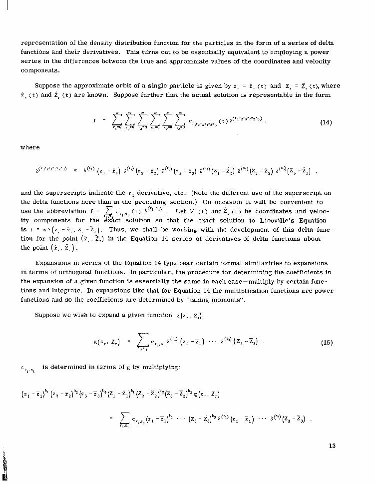
representation of the density distribution function for the particles in the form of a ser ies of delta functions and their derivatives. This turns out to be essentially equivalent to employing a power ser ies in the differences between the true and approximate values of the coordinates and velocity components.

Suppose the approximate orbit of a single particle is given by Z , = z , ( t ) and z, = 2, (t), where Z r ( t ) and tr ( t ) a r e known. Suppose further that the actual solution is representable in the form

where

and the superscripts indicate the r derivative, etc. (Note the different use of the superscript on the delta functions here than in the preceding section.) On occasion it will be convenient to use the abbreviation f = c ~ ~ , ~ ~ ( t ) 8 ( r i * s i ) . Let 1, ( t ) and ?r ( t ) be coordinates and veloc- i ty components for the &&ct solution so that the exact solution to Liouville's Equation is f = m 6 ( z r - Z r , Z r - Z r ) . Thus, we shall be working with the development of this delta function for the point (2r , Z , ) in the Equation 14 ser ies of derivatives of delta functions about the point ( Z r , ir) .

b

,L

Expansions in ser ies of the Equation 14 type bear certain formal similarities to expansions in terms of orthogonal functions. In particular, the procedure for determining the coefficients in the expansion of a given function is essentially the same in each case-multiply by certain functions and integrate. In expansions like that for Equation 14 the multiplication functions a r e power functions and so the coefficients are determined by "taking moments".

Suppose we wish to expand a given function g ( z r , zr):

c r . , s . I , is determined in terms of g by multiplying:

(21 -Qhl (z* - % ) h Z ( 2 3 - Z J h 3 ( Z 1 -zl)kl(z* - Z 2 p ( Z 3 - z 3 ) k 3 g ( z r , - -

z.)

13

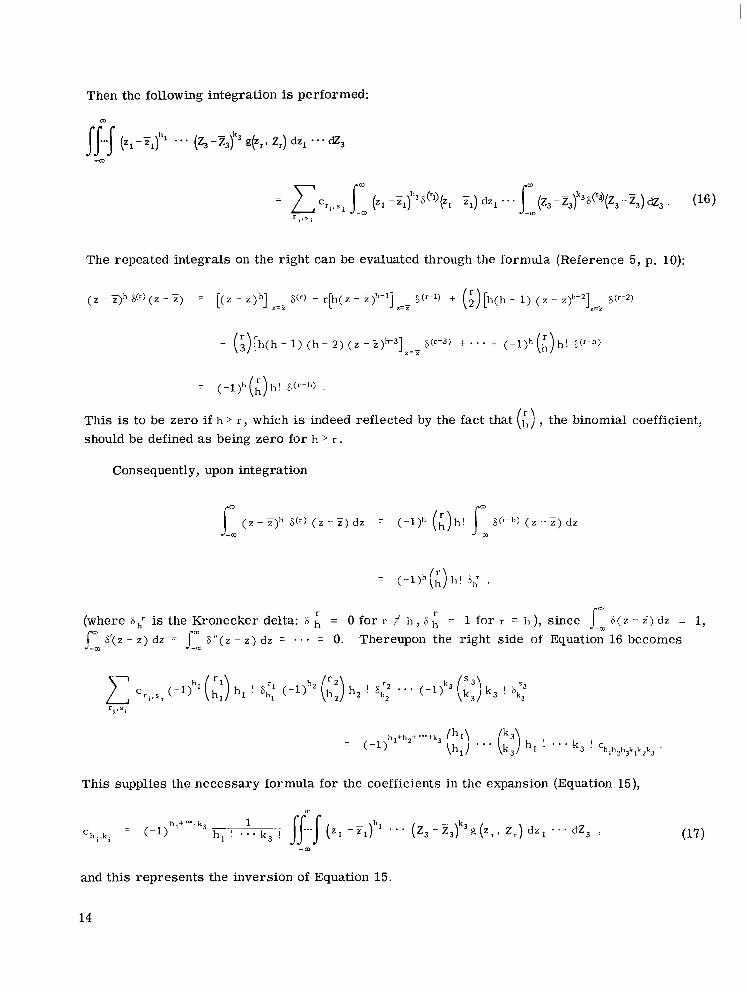
Then the following integration is performed:

m

The repeated integrals on the right can be evaluated through the formula (Reference 5, p. 10):

This is to be zero i f h > r , which is indeed reflected by the fact that (;I) , the binomial coefficient, should be defined as being zero for h > r .

Consequently, upon integration

= (-l)h(i) h! 6; ,

(where S t is the Kronecker delta: 6 ;I = 0 for r # h , 6 ;I = 1 for r = h ), since Jl S( z - Z) dz = 1, J-:s'(z-z)dz = J-:8 ' ' (z -z)dz = ... - - 0. Thereupon the right side of Equation 16 becomes

= (-1) h1th2t"'tk3 (L:) . . . (ti:) h , ! . . . k 3 1 ' hlh2h3klk2k3

This supplies the necessary formula for the coefficients in the expansion (Equation 15),

and this represents the inversion of Equation 15.

14

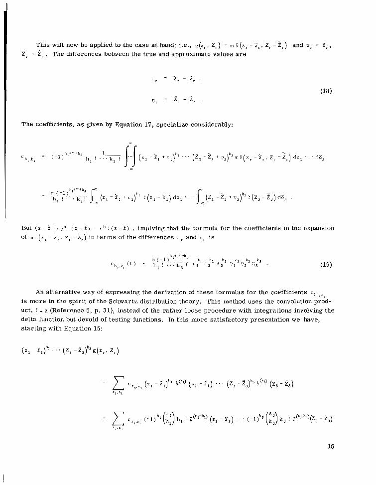
I This will now be applied to the case at hand; i.e., g ( z , , Z r ) = rn 6 ( z r - g r , Zr - Z r ) and zr = i r , -

- Z r = ir . The differences between the true and approximate values a r e

The coefficients, as given by Equation 17, specialize considerably:

But ( Z - 2 + ) h - ( z - 2 ) t .'( z - 2 ) , implying that the formula for the coefficients in the expansion of 111 '1 ( Z - Z r l z r - ? r ) in terms of the differences 6 and T~ is

An alternative way of expressing the derivation of these formulas for the coefficients is more in the spirit of the Schwartz distribution theory. This method uses the convolution product, f * g (Reference 5, p. 31), instead of the rather loose procedure with integrations involving the delta function but devoid of testing functions. In this more satisfactory presentation w e have, starting with Equation 15:

15

I

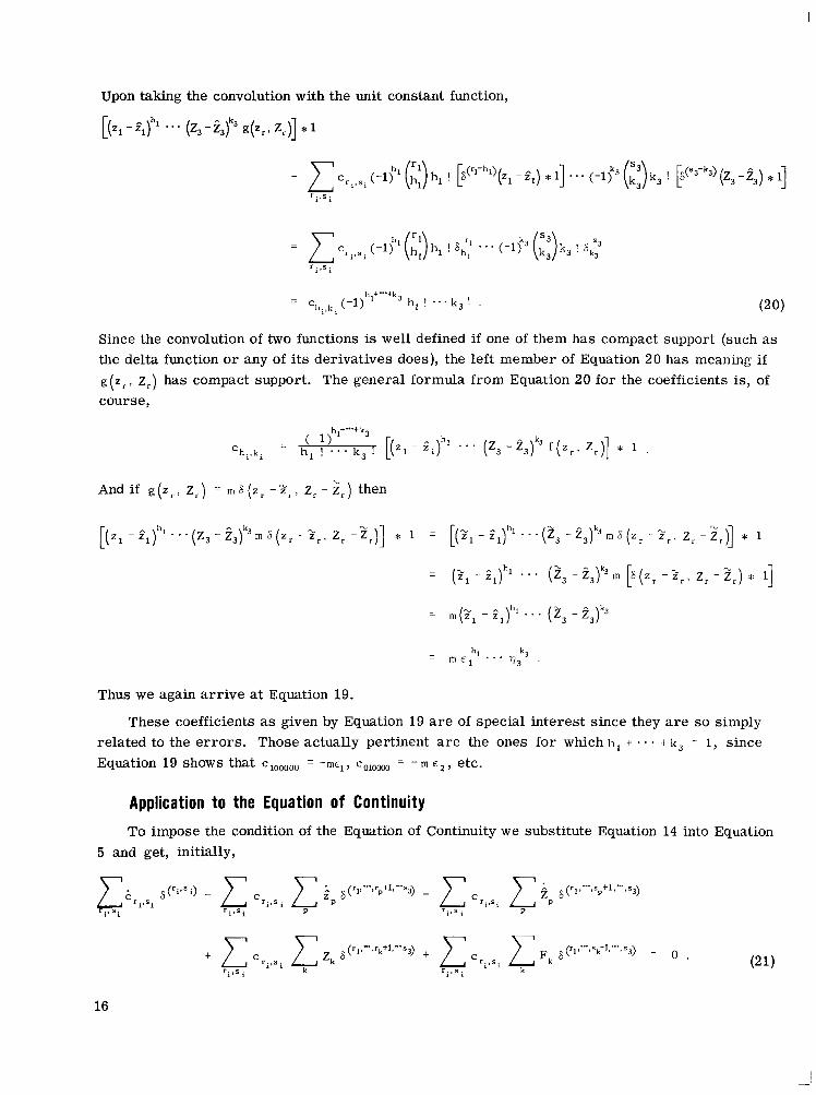
Upon taking the convolution with the unit constant function,

[(z, -5,p * * . ( Z 3 - i 3 F g(Z,, z,)] * 1

Since the convolution of two functions is well defined if one of them has compact support (such as the delta function or any of its derivatives does), the left member of Equation 20 has meaning if g ( z , , zr) has compact support. The general formula from Equation 20 for the coefficients is, of course,

Andif g ( z r , z , ) = m 8 ( z r - l r , z r - z r ) then

Thus we again arrive at Equation 19.

These coefficients as given by Equation 19 a r e of special interest since they a r e so simply related to the errors. Those actually pertinent are the ones for which h , t . . . t k, = 1 , since Equation 19 shows that clooooo = - m E l , coloooo = - m c 2 , etc.

Application to the Equation of Continuity To impose the condition of the Equation of Continuity we substitute Equation 14 into Equation

5 and get, initially,

C * , I s ( r i * s i ) - ip 8(rl,***,rp+1,"~ 3) - c r i , s i c ip S ( r l , %+1*"3) ...

r . , s . ' r . , s .

P * I r.,s.

I I r . , s . L 1

16

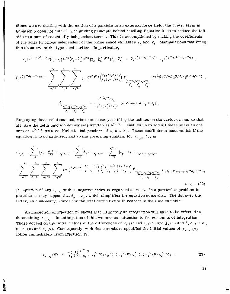
(Since we are dealing with the motion of a particle in an external force field, the dU/dzr term in Equation 5 does not enter.) The guiding principle behind handling Equation 21 is to reduce the left side to a sum of essentially independent terms. This is accomplished by making the coefficients of the delta functions independent of the phase space variables z r and zr. Manipulations that bring this about a r e of the type used earlier. In particular,

Employing these relations and, where necessary, shifting the indices on the various sums so that all have the delta function derivatives written as b ( r i * s i, enables u s to add all these sums as one sum on with coefficients independent of z and Z r . These coefficients must vanish if the equation is to be satisfied, and so the governing equation for c r ( t ) is

1 ' s i

An inspection of Equation 22 shows that ultimately an integration will have to be effected in determining c , , B , . In anticipation of this we turn our attention to the constants of integration. These depend on the initial values of the differences of Zr (t) and f r ( t ) , and ?r ( t ) and 2r ( t ) ; i.e., on E ( 0 ) and T~ (0). Consequently, with these numbers specified the initial values of c r , ( t )

follow immediately from Equation 19:

I ,

I * s i

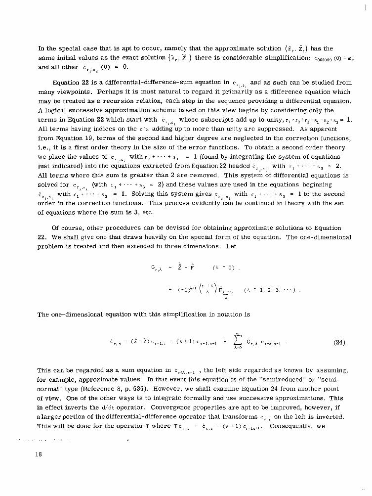
In the special case that is apt to occur, namely that the approximate solution (Z, , ir) has the same initial values as the exact solution (Sr , z,) there is considerable simplification: c~~~~~~ (0 ) = m ,

and all other c , , , ~ , ( 0 ) = 0.

-L

I 3

Equation 22 is a differential-difference-sum equation in c ~ , , ~ , and as such can be studied from many viewpoints. Perhaps it is most natural to regard it primarily as a difference equation which may be treated as a recursion relation, each step in the sequence providing a differential equation. A logical successive approximation scheme based on this view begins by considering only the t e rms in Equation 22 which start with & r , , s , whose subscripts add up to unity, rl + r 2 t r 3 + S 1 i s 2 t s3 = 1. All terms having indices on the c' s adding up to more than unity are suppressed. As apparent from Equation 19, terms of the second and higher degree are neglected in the correction functions; i.e., it is a first order theory in the size of the e r r o r functions. To obtain a second order theory we place the values of c ~ ~ , ~ ~ with r + . . + s 3 = 1 (found by integrating the system of equations just indicated) into the equations extracted fromEquation 22 headed C, , , 5 . with r + . . . + s 3 = 2. All terms where this sum is greater than 2 are removed. This system of differential equations is solved for c ~ , , ~ , (with r l + . . . + s 3 = 2) and these values are used in the equations beginning A r , , s , with r l t ... + s 3 = 1. Solving this system gives c ~ ; , ~ , with r l t . . . + s 3 = 1 to the second order in the correction functions. This process evidently can be continued in theory with the set of equations where the sum is 3, etc.

. I

, I

, I

, I

X I

Of course, other procedures can be devised for obtaining approximate solutions to Equation 22. We shall give one that draws heavily on the special form of the equation. problem is treated and then extended to three dimensions. Let

The one-dimensional equation with this simplification in notation is

The one-dimensional

. . ) .

(24)

This can be regarded as a sum equation in crtX,s-l , the left side regarded as known by assuming, for example, approximate values. In that event this equation is of the "semireduced" or "semi- normal" type (Reference 8, p. 535). However, we shall examine Equation 24 from another point of view. One of the other ways is to integrate formally and use successive approximations. This in effect inverts the d/dt operator. Convergence properties are apt to be improved, however, if a larger portion of thedifferential-difference operator that transforms c r , , on the left is inverted. This will be done for the operator T where T c r , s = & r , s - ( s + 1) c , - ~ , ~ + ~ . Consequently, we

18

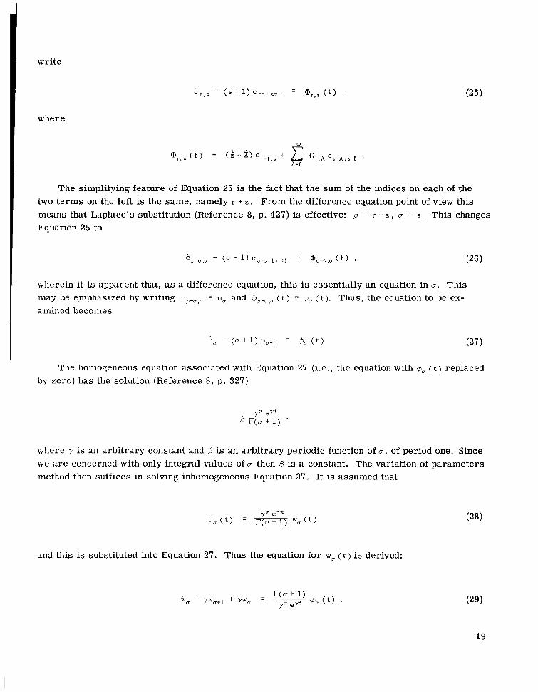
write

where

The simplifying feature of Equation 25 is the fact that the sum of the indices on each of the two terms on the left is the same, namely r t S . From the difference equation point of view this means that Laplace's substitution (Reference 8, p. 427) is effective: p = r + S , u = s . This changes Equation 25 to

wherein it is apparent that, as a difference equation, this is essentially an equation in 0. This may be e.mphasized by writing c ~ - ~ , , = U, and ( t ) = @u ( t ) . Thus, the equation to be examined becomes

The homogeneous equation associated with Equation 27 (i.e., the equation with eU ( t ) replaced by zero) has the solution (Reference 8, p. 327)

where y is an arbitrary constant and 3 is an arbitrary periodic function of D , of period one. Since we are concerned with only integral values of D then p is a constant. The variation of parameters method then suffices in solving inhomogeneous Equation 27. It is assumed that

and this is substituted into Equation 27. Thus the equation for W, ( t ) is derived:

19

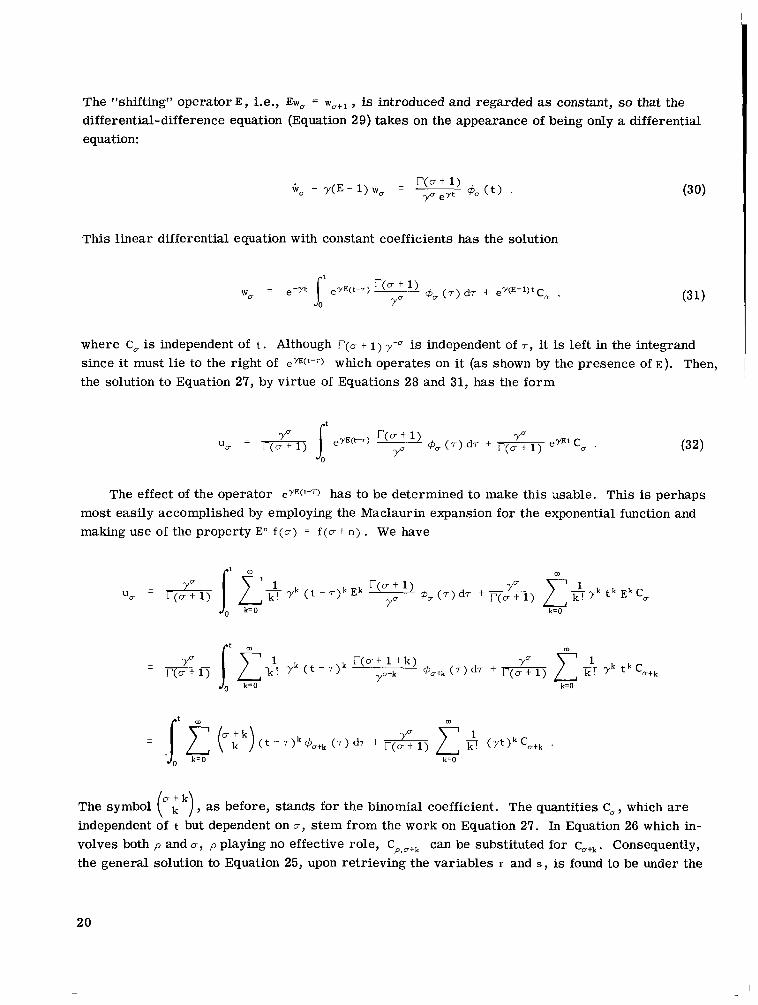
The "shifting" operator E , i.e., Ew, = w,+~ , is introduced and regarded as constant, so that the differential-difference equation (Equation 29) takes on the appearance of being only a differential equation:

6, -

This linear differential equation with constant coefficients has the solution

where C, is independent of t . Although r ( m t 1) y-u is independent of T, it is left in the integrand since it must lie to the right of emt") which operates on it (as shown by the presence of E ) . Then, the solution to Equation 27, by virtue of Equations 28 and 31, has the form

The effect of the operator erE(t-7) has to be determined to make this usable. This is perhaps most easily accomplished by employing the Maclaurin expansion for the exponential function and making use of the property E" f(o) = f ( o f n ) . We have

The symbol ( k ) , as before, stands for the binomial coefficient. The quantities C,, which a r e independent of t but dependent on u , stem from the work on Equation 27. In Equation 26 which involves both p and U , p playing no effective role, Cp,,+k can be substituted for c ,+~. consequently, the general solution to Equation 25, upon retrieving the variables r and S , is found to be under the

u + k

20

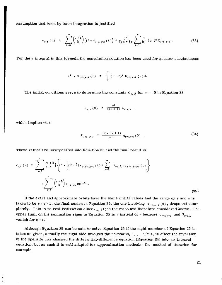
assumption that term by term integration is justified

For the T integral in this formula the convolution notation has been used for greater succinctness:

The initial conditions serve to determine the constants C r . s; for t = 0 in Equation 33

which implies that

r(s f k f 1) 'rts,stk X .,,stk ' r - k , s t k (O) (34 1

These values are incorporated into Equation 33 and the final result is

If the exact and approximate orbits have the same initial values and the range on r and s is taken to be r + s 2 1, the final ser ies in Equation 35, the one involving c ~ - ~ , ~ + ~ (0) , drops out completely. This is no real restriction since coo ( t ) is the mass and therefore considered known. The upper limit on the summation signs in Equation 35 is r instead of m because c ~ - ~ , ~ + ~ and GI_,,* vanish for k > r .

Although Equation 35 can be said to solve Equation 25 if the right member of Equation 25 is taken as given, actually the right side involves the unknowns, c r , s . Thus, in effect the inversion of the operator has changed the differential-difference equation (Equation 24) into an integral equation, but as such it is well adapted for approximation methods, the method of iteration for example.

21

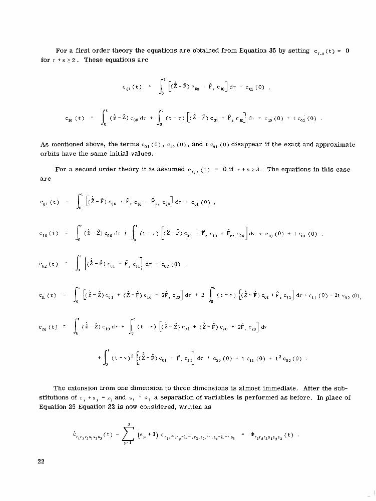
For a first order theory the equations are obtained from Equation 35 by setting ( t ) = 0 for r + s 2 . These equations a r e

As mentioned above, the terms col ( 0 ) , cl0 ( 0 ) , and t col ( 0 ) disappear if the exact and approximate orbits have the same initial values.

For a second order theory it is assumed c r , ( t ) = 0 if r + s 2 3 . The equations in this case a r e

Cl0 ( t ) = [ (i-2) Coo d7 + ( t - 7 ) (2-e) Coo + ez cl0 + 6,, c,,]di + cl0 (0) + t col (0 ) , I [ '

The extension from one dimension to three dimensions is almost immediate. After the substitutions of r t s i = pi and s i = D~ a separation of variables is performed as before. In place of Equation 25 Equation 22 is now considered, written as

22

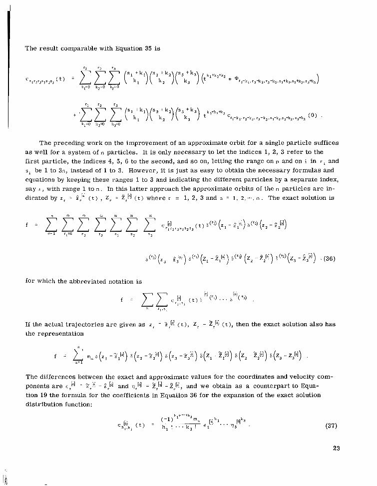
The result comparable with Equation 35 is

The preceding work on the improvement of an approximate orbit for a single particle suffices as well for a system of n particles. It is only necessary to let the indices 1, 2, 3 refer to the first particle, the indices 4, 5, 6 to the second, and so on, letting the range on p and on i in r and s i be 1 to 311, instead of 1 to 3. However, it is just as easy to obtain the necessary formulas and equations by keeping these ranges 1 to 3 and indicating the different particles by a separate index, say L ~ , with range 1 to n. In this latter approach the approximate orbits of the n particles are indicated by z r = ( t ) , Z r = 2,[4 ( t ) where r = 1, 2, 3 and a = 1 , 2,- . , n . The exact solution is

for which the abbreviated notation is

If the actual trajectories are given as z r = Zr[d ( t ), Z r = ;?r[.3 ( t ) , then the exact solution also has the representation

The differences between the exact and approximate values for the coordinates and velocity components a r e e ? = 2rb] - 2,[4 and v,[d = ?r[4 - 2r[4, and we obtain as a counterpart to Equa- tion 19 the formula for the coefficients in Equation 36 for the expansion of the exact solution distribution function:

23

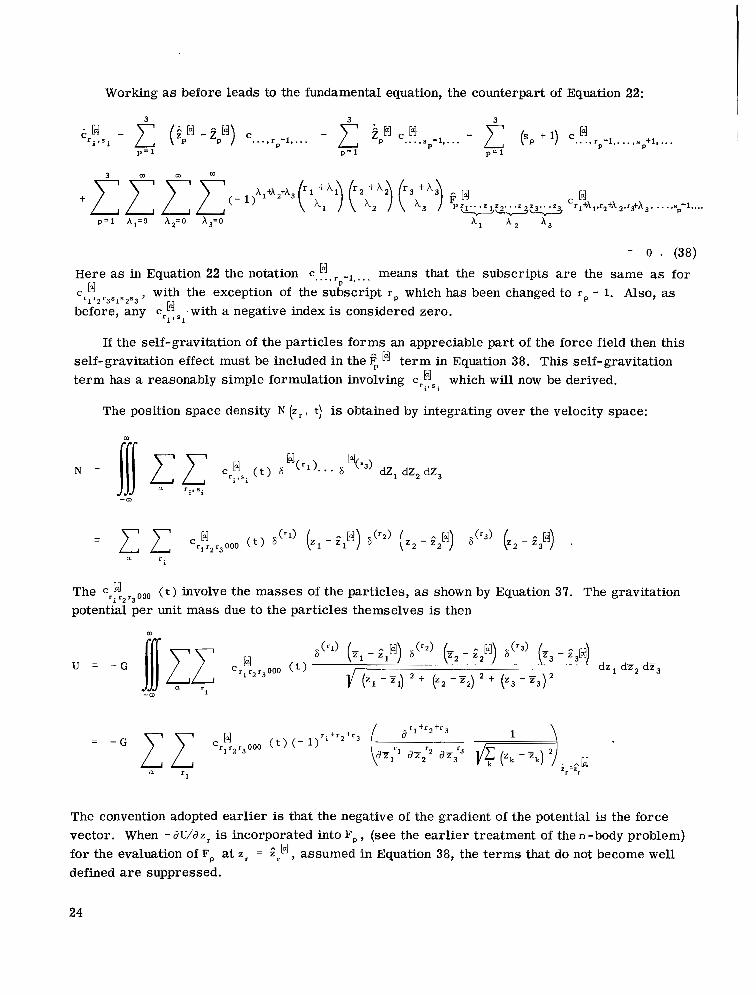
Working as before leads to the fundamental equation, the counterpart of Equation 22:

3 * M - ( i P H - iP"> - 2 ;PI 14 - 2 k p + 1) c.. w ., rp-l.. .. ,sp+l, .. .

' r i . s i ' ..., r -1 ,... p ' ..., s -1 ,... p = 1 p = 1 p = 1

p = l h,=O X,=O h3=0

= 0 . (38)

Here as in Equation 22 the notation c..., -l,. .. means that the subscripts are the same as for

before, any c,F4 .with a negative index is considered zero.

w E4 with the exception of the subscript rp which has been changed to rp - 1. Also, as

P

'1'2'3s1s2s3 ' l P s i

If the self-gravitation of the particles forms an appreciable part of the force field then this self-gravitation effect must be included in the term in Equation 38. This self-gravitation term has a reasonably simple formulation involving crysi which will now be derived.

The position space density N ( z r , t) is obtained by integrating over the velocity space:

a r .

The cr!2r3000 ( t ) involve the masses of the particles, as shown by Equation 37. The gravitation potential per unit mass due to the particles themselves is then

m

The convention adopted earlier is that the negative of the gradient of the potential is the force vector. When - dU/dzr is incorporated into FP , (see the earlier treatment of the n -body problem) for the evaluation of FP at z r = s,', assumed in Equation 38, the terms that do not become well defined are suppressed.

24

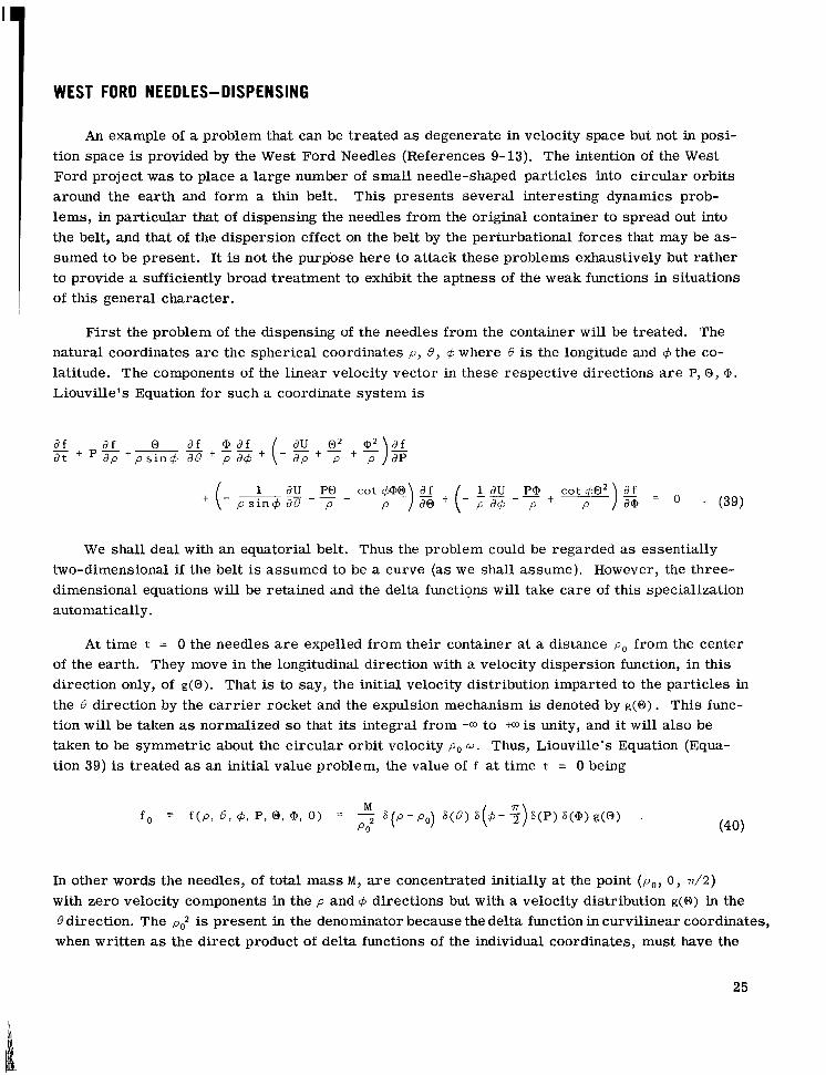
WEST FORD NEEDLES-DISPENSING

An example of a problem that can be treated as degenerate in velocity space but not in position space is provided by the West Ford Needles (References 9-13). The intention of the West Ford project was to place a large number of small needle-shaped particles into circular orbits around the earth and form a thin belt. This presents several interesting dynamics problems, in particular that of dispensing the needles from the original container to spread out into the belt, and that of the dispersion effect on the belt by the perturbational forces that may be assumed to be present. It is not the purpose here to attack these problems exhaustively but rather to provide a sufficiently broad treatment to exhibit the aptness of the weak functions in situations of this general character.

First the problem of the dispensing of the needles from the container will be treated. The natural coordinates are the spherical coordinates p, 0 , + where B is the longitude and + the co- latitude. The components of the linear velocity vector in these respective directions are P, 0, cp. Liouville's Equation for such a coordinate system is

1 dU PO cot @0 1 dU P@ + cot 40' ) 2 = P ' (39)

We shall deal with an equatorial belt. Thus the problem could be regarded as essentially two-dimensional if the belt is assumed to be a curve (as we shall assume). However, the three- dimensional equations will be retained and the delta functions wil l take care of this specialization automatically.

At time t = 0 the needles are expelled from their container at a distance po from the center of the earth. They move in the longitudinal direction with a velocity dispersion function, in this direction only, of g(O) . That is to say, the initial velocity distribution imparted to the particles in the B direction by the carrier rocket and the expulsion mechanism is denoted by g ( 0 ) . This function will be taken as normalized so that its integral from -a to +a is unity, and it will also be taken to be symmetric about the circular orbit velocity p, w . Thus, Liouville's Equation (Equa- tion 39) is treated as an initial value problem, the value of f at time t = 0 being

In other words the needles, of total mass M , are concentrated initially at the point (p,, 0 , 7d2)

with zero velocity components in the p and + directions but with a velocity distribution g ( O ) in the Bdirection. The pt is present in the denominator because the delta function in curvilinear coordinates, when written as the direct product of delta functions of the individual coordinates, must have the

25

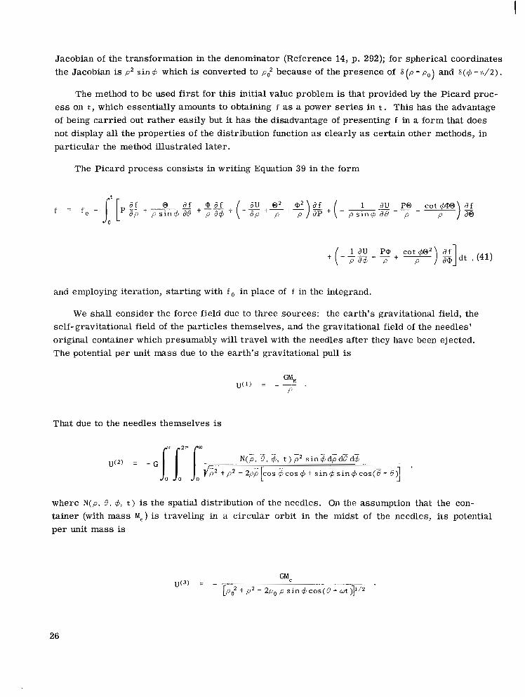
Jacobian of the transformation in the denominator (Reference 14, p. 292); for spherical coordinates the Jacobian is p2 s i n 4 which is converted to p: because of the presence of 6 ( p - p o ) and 8(+ - n / 2 ) .

The method to be used first for this initial value problem is that provided by the Picard proc- e s s on t , which essentially amounts to obtaining f as a power ser ies in t , This has the advantage of being carried out rather easily but it has the disadvantage of presenting f in a form that does not display all the properties of the distribution function as clearly as certain other methods, in particular the method illustrated later.

The Picard process consists in writing Equation 39 in the form

f (-7s 1 dU - 7 P@ cot -) P &3' g ] d t , (41)

and employing iteration, starting with f , i n place of f in the integrand.

We shall consider the force field due to three sources: the earth's gravitational field, the self-gravitational field of the particles themselves, and the gravitational field of the needles' original container which presumably will travel with the needles after they have been ejected. The potential per unit mass due to the earth's gravitational pull is

That due to the needles themselves is

where N ( p , 8 , 4, t ) is the spatial distribution of the needles. On the assumption that the container (with mass Mc) is traveling in a circular orbit in the midst of the needles, its potential per unit mass is

26

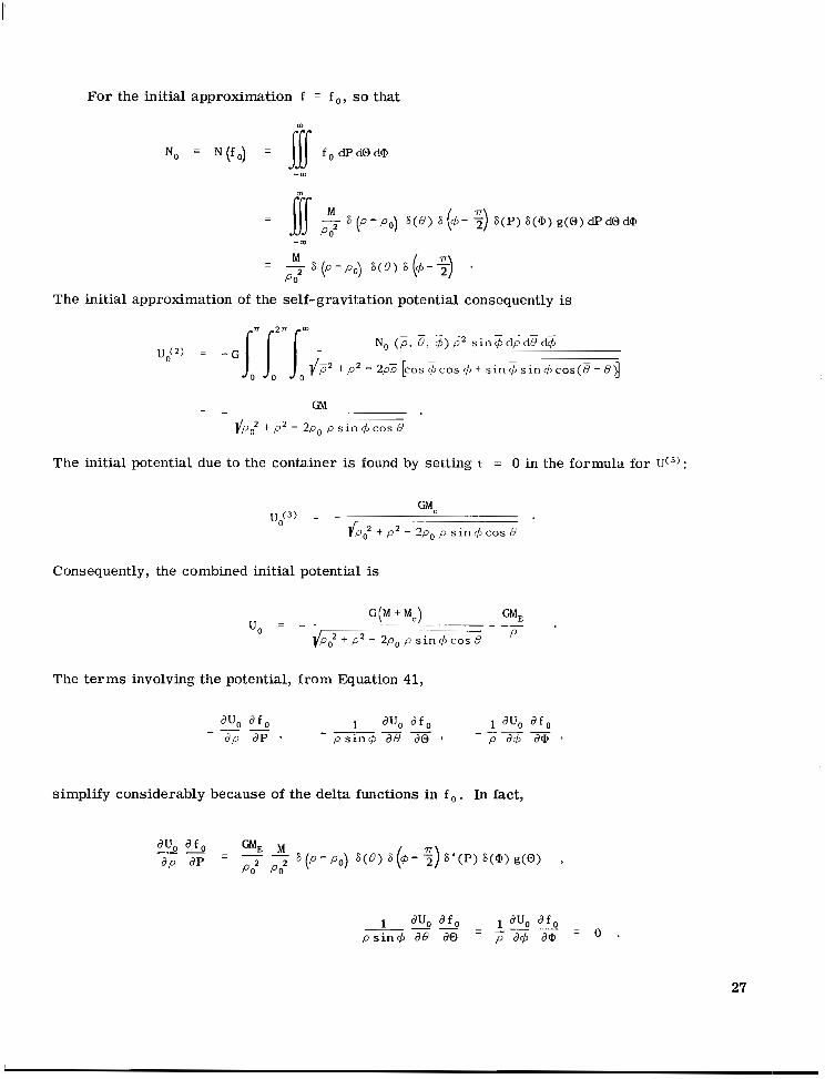
For the initial approximation f = f,, so that

No E N ( f o ) = 11 f ,dPd@d@

The initial approximation of the self-gravitation potential consequently is

The initial potential due to the container is found by setting t = 0 in the formula for u ( ~ ) :

Consequently, the combined initial potential is

The terms involving the potential, from Equation 41,

JU, J f , 1 JUO J f o 1 JUO J f o " "" - J p J P ' p s i n + JQ J @ 9 p J+ J @ '

-" -

simplify considerably because of the delta functions in f , . In fact,

1 JU, J f o - 1 JUO J f o - p sinq5 J0 J@ - p Jq5 J @

- - 0 .

27

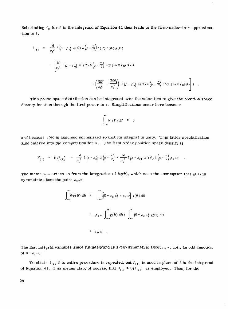
Substituting f for f in the integrand of Equation 4 1 tion to f :

then leads to the first-order-in-t approxima-

This phase space distribution can be integrated over the velocities to give the position space density function through the first power in t . Simplifications occur here because

and because g ( 0 ) is assumed normalized so that its integral is unity. This latter specialization also entered into the computation for No. The first order position space density is

The factor po w arises as from the integration of Og(O) , which uses the assumption that g ( 0 ) is symmetric about the point p o w :

= po w J g ( O ) dO+ J (O - p 0 b) g ( O ) dO -a -m

The last integral vanishes since its integrand is skew-symmetric about po &I; i.e., an odd function of 0 - po w .

To obtain f ( 2 ) this entire procedure is repeated, but f is used in place of f in the integrand of Equation 41. This means also, of course, that U ( l ) U ( f ( , ) ) is employed. Thus, for the

28

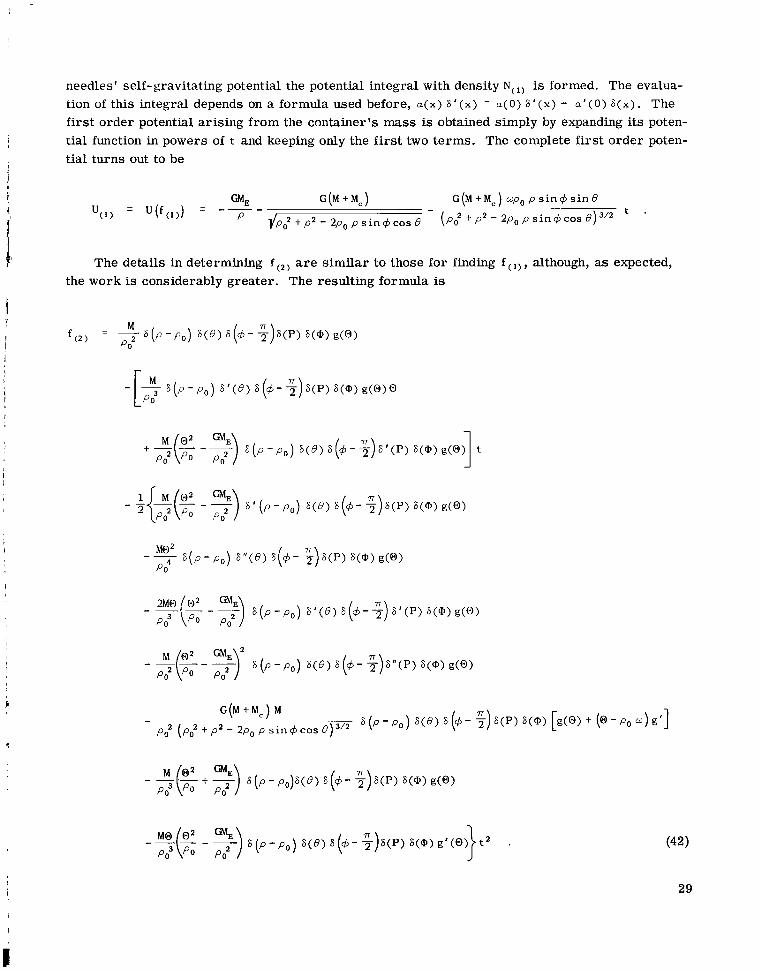
needles' self-gravitating potential the potential integral with density N ( l ) is formed. The evaluation of this integral depends on a formula used before, .(x) S'(X) = a ( 0 ) 8'(x) - a ' ( 0 ) 6 ( x ) . The first order potential arising from the container's mass is obtained simply by expanding its potential function in powers of t and keeping only the first two terms. The complete first order potential turns out to be

The details in determining f (z) are similar to those for finding f ( 1), although, as expected, the work is considerably greater. The resulting formula is

I

4

(42 1

29 I

E

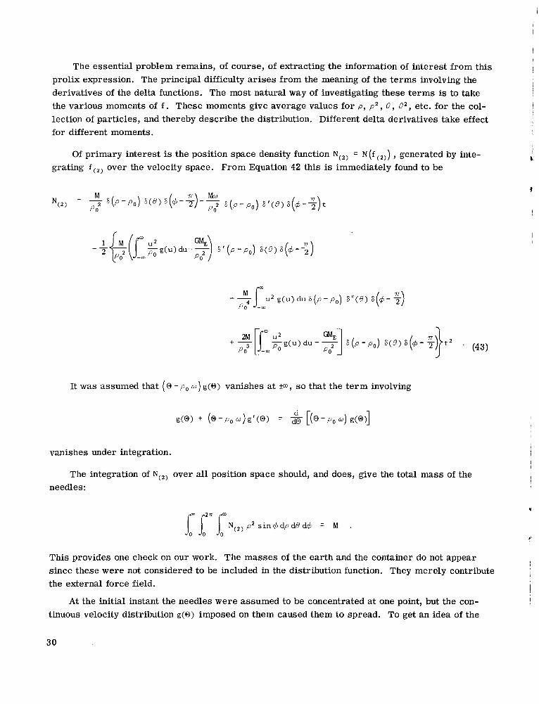
The essential problem remains, of course, of extracting the information of interest from this ! prolix expression. The principal difficulty arises from the meaning of the terms involving the

I derivatives of the delta functions. The most natural way of investigating these terms is to take 1 the various moments of f . These moments give average values for p, pz , 8, 8' , etc. for the col- I lection of particles, and thereby describe the distribution. Different delta derivatives take effect I for different moments.

I I 1

Of primary interest is the position space density function N(') N ( f , generated by inte- I L . grating f (') over the velocity space. From Equation 42 this is immediately found to be

It was assumed that ( 0 - po w ) g ( 0 ) vanishes at +a,, so that the term involving

vanishes under integration.

The integration of N(2) over all position space should, and does, give the total mass of the needles:

This provides one check on our work. The masses of the earth and the container do not appear since these were not considered to be included in the distribution function. They merely contribute the external force field.

At the initial instant the needles were assumed to be concentrated at one point, but the con- 1 tinuous velocity distribution g ( 0 ) imposed on them caused them to spread. To get an idea of the

30

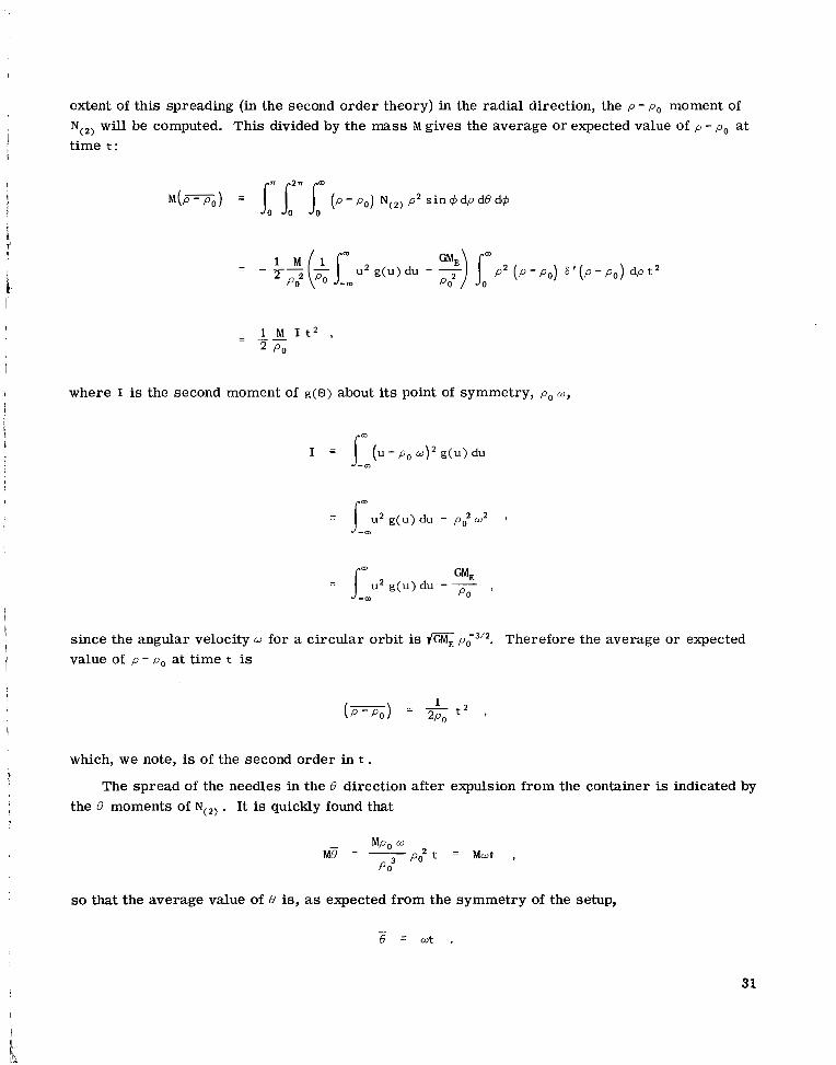
extent of this spreading (in the second order theory) in the radial direction, the p - p0 moment of N c z ) will be computed. This divided by the mass M gives the average or expected value of p - po at time t :

" - 1 M I t Z , - * P O

i

where I is the second moment of g ( 0 ) about its point of symmetry, po W ,

( P - P o ) = - t Z , I

*PO

which, we note, is of the second order in t . The spread of the needles in the B direction after expulsion from the container is indicated by

the B moments of N(z) . It is quickly found that

so that the average value of B is, as expected from the symmetry of the setup,

31

or

= . POZ 2

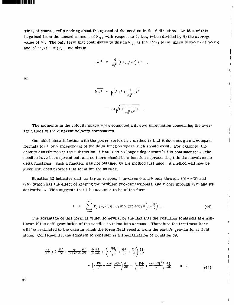
The moments in the velocity space when computed will give information concerning the average values of the different velocity components.

Our chief dissatisfaction with the power series in t method is that it does not give a compact formula for f or N independent of the delta function where such should exist. For example, the density distribution in the B direction at time t is no longer degenerate but is continuous; i.e. the needles have been spread out, and so there should be a function representing this that involves no delta functions. Such a function was not obtained by the method just used. A method will now be given that does provide this form for the answer.

Equation 42 indicates that, as far as it goes, f involves + and @ only through S(+ - d 2 ) and S ( @ ) (which has the effect of keeping the problem two-dimensional), and P only through S(P) and its derivatives. This suggests that f be assumed to be of the form

The advantage of this form is offset somewhat by the fact that the resulting equations are nonlinear if the self-gravitation of the needles is taken into account. Therefore the treatment here will be restricted to the case in which the force field results from the earth's gravitational field alone. Consequently, the equation to consider is a specialization of Equation 39:

32

i

P

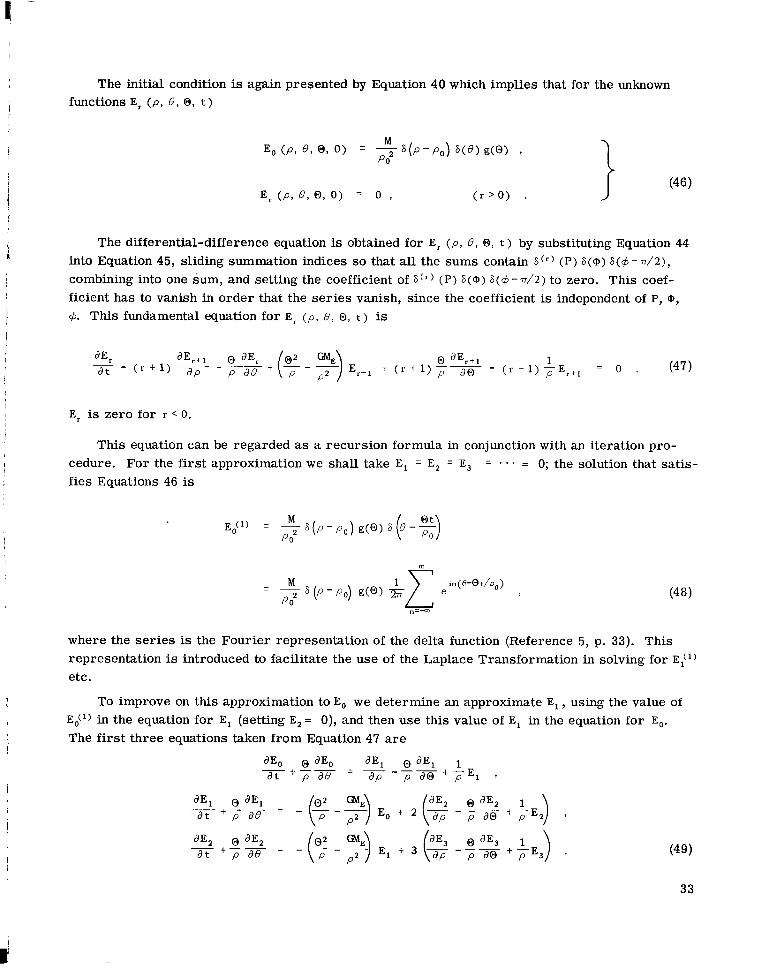
The initial condition is again presented by Equation 40 which implies that for the unknown functions Er ( P , 0 , 0, t)

Er is zero for r < 0.

This equation can be regarded as a recursion formula in conjunction with an iteration procedure. For the first approximation we shall take E, = E, = E, = . . . = 0; the solution that satisfies Equations 46 is

where the series is the Fourier representation of the delta function (Reference 5, p. 33). This representation is introduced to facilitate the use of the Laplace Transformation in solving for E:,) etc.

TO improve on this approximation to E, we determine an approximate E, , using the value of E,,(') in the equation for E, (setting E, = 0), and then use this value of E, in the equation for E,.

The first three equations taken from Equation 47 a r e

(49)

33

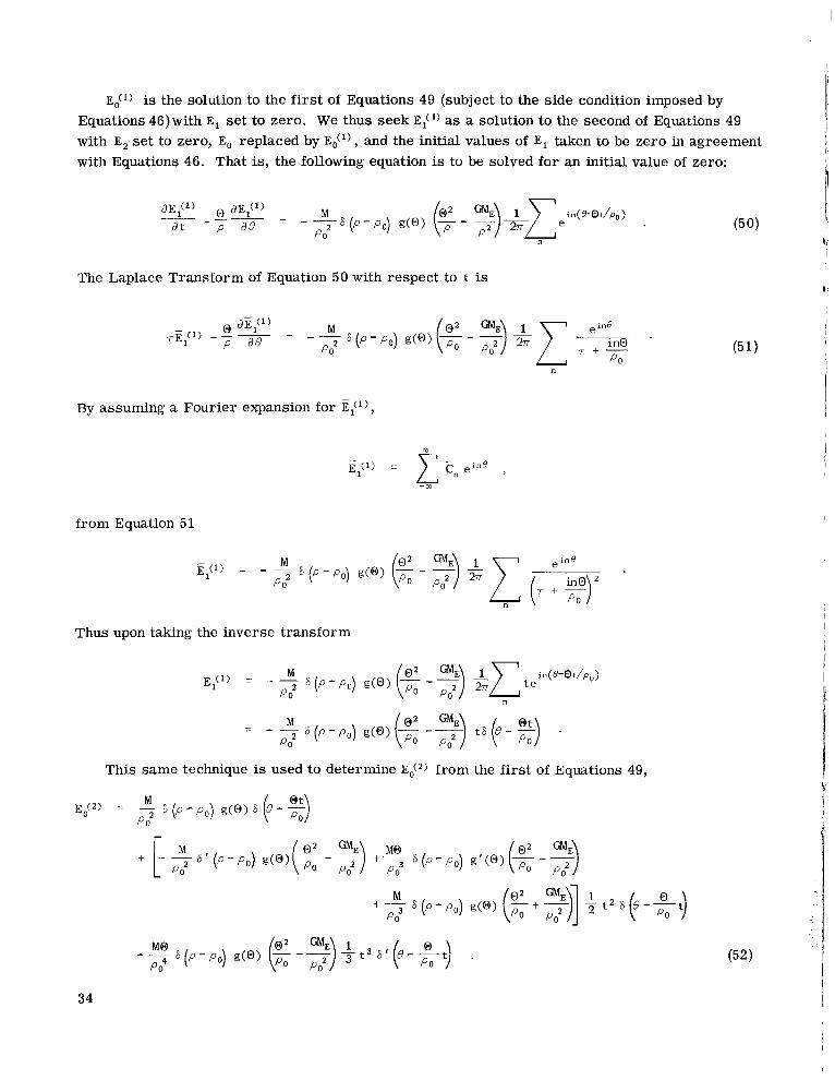
Ed') is the solution to the first of Equations 49 (subject to the side condition imposed by Equations 46) with E, set to zero. We thus seek E,( ') as a solution to the second of Equations 49 with E, set to zero, E, replaced by Ed ' ) , and the initial values of E, taken to be zero in agreement with Equations 46. That is, the following equation is to be solved for an initial value of zero:

The Laplace Transform of Equation 50 with respect to t is

I

By assuming a Fourier expansion for E,(1),

from Equation 51

Thus upon taking the inverse transform

This same technique is used to determine E d Z ) from the first of Equations 49,

34

r

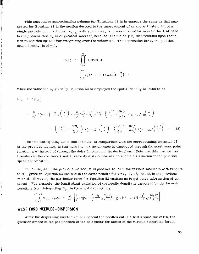
This successive approximation scheme for Equations 49 is in essence the same as that suggested for Equation 22 in the section devoted to the improvement of an approximate orbit of a single particle or n particles. c ~ , , ~ , with r t . . . t s 3 = 1 was of greatest interest for that case. In the present case E, is of greatest interest, because it is the only E r that remains upon reduc- tion to position space after integrating over the velocities. The expression for N, the position space density, is simply

1 1

N ( f ) = (1 fdPdOd@

- m

When the value for E, given by Equation 52 is employed the spatial density is found to be

The interesting thing about this formula, in comparison with the corresponding Equation 43 of the previous method, is that here the ( 7 , t dependence is expressed through the continuous point function g ( u ) instead of through the delta function and its derivatives. Note that this method has transferred the continuous initial velocity distribution in 0 to such a distribution in the position space coordinate :>.

Of course, as in the previous method, it is possible to form the various moments with respect to N ( z ) given in Equation 53 and obtain the same results for p ->;, 8 , ( j2 , etc. as in the previous method. However, the particular form for Equation 53 enables us to get other information of interest. For example, the longitudinal variation of the needle density is displayed by the fornlula resulting from integrating N ( z ) in the p and 6 directions:

WEST FORD NEEDLES-DISPERSION

After the dispensing mechanism has spread the needles out in a belt around the earth, the question a r i s e s of the permanence of the belt under the action of the various disturbing forces.

35

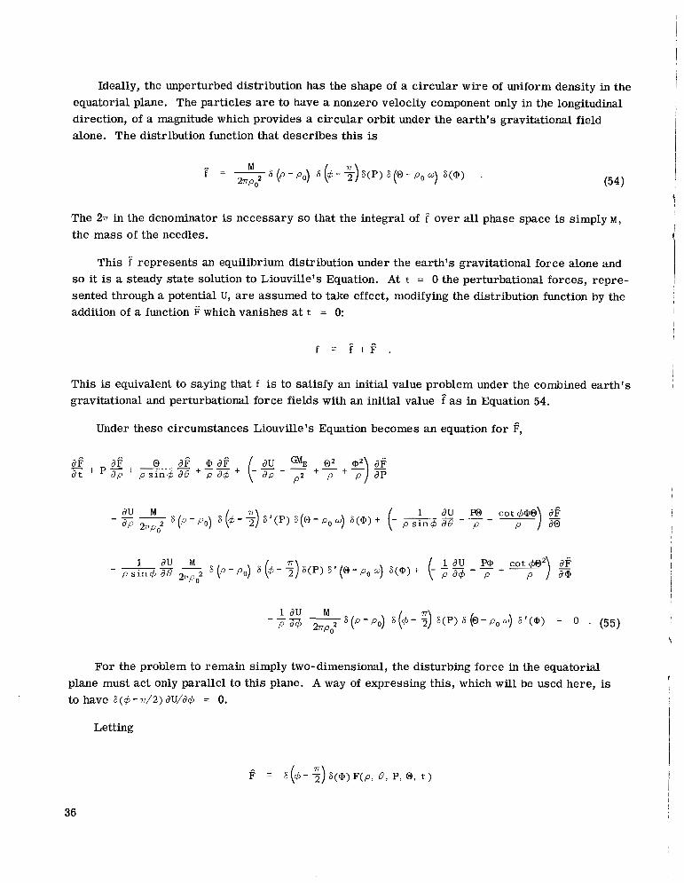
Ideally, the unperturbed distribution has the shape of a circular wire of uniform density in the equatorial plane. The particles are to have a nonzero velocity component only in the longitudinal direction, of a magnitude which provides a circular orbit under the earth's gravitational field alone. The distribution function that describes this is

(54 1

The 271 in the denominator is necessary so that the integral of f over all phase space is simply M, the mass of the needles.

This 2 represents an equilibrium distribution under the earth's gravitational force alone and so it is a steady state solution to Liouville's Equation. At t = 0 the perturbational forces, represented through a potential U, are assumed to take effect, modifying the distribution function by the addition of a function which vanishes at t = 0:

f = F + F .

This is equivalent to saying that f is to satisfy an initial value problem under the combined earth's gravitational and perturbational force fields with an initial value ? as in Equation 54.

Under these circumstances Liouville's Equation becomes an equation for f,

For the problem to remain simply two-dimensional, the disturbing force in the equatorial plane must act only parallel to this plane. A way of expressing this, which will be used here, is to have S(4- d 2 ) aWa4 = 0.

Letting

36

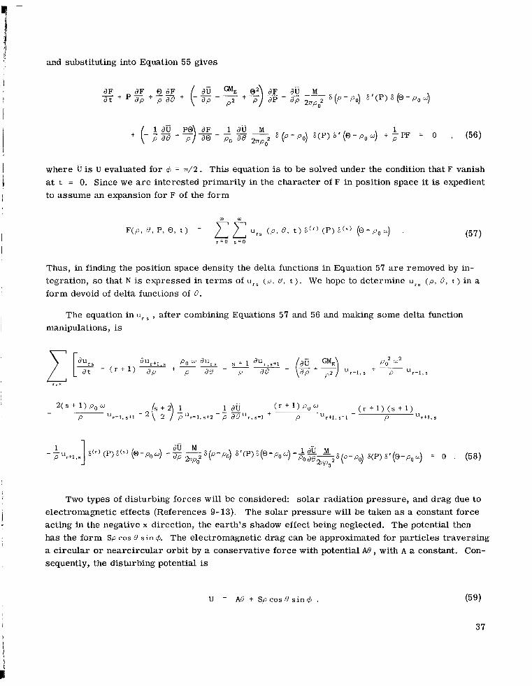
and substituting into Equation 55 gives

where is U evaluated for 4 = ~ / 2 . This equation is to be solved under the condition that F vanish at t = 0. Since we are interested primarily in the character of F in position space it is expedient to assume an expansion for F of the form

Thus, in finding the position space density the delta functions in Equation 57 are removed by integration, so that N is expressed in terms of u r s ( 0 , a, t ) . We hope to determine u r S ( p , 8, t ) in a form devoid of delta functions of 8.

The equation in ur , after combining Equations 57 and 56 and making some delta function manipulations, is

" I p U r + l , s S ( ' ) ( P ) S ( ~ ) ( o - p 0 w ) " -S(p-po) S'(P)S(o-p,w)-" - 1 d 6 M 1 J U M

dp a p t p o a e y S ( O - p o ) S(P)S'(@-p,a) = 0 . (58) 2 T "

Two types of disturbing forces will be considered: solar radiation pressure, and drag due to electromagnetic effects (References 9-13). The solar pressure will be taken as a constant force acting in the negative x direction, the earth's shadow effect being neglected. The potential then has the form Sp cos 8 s i n 4. The electromagnetic drag can be approximated for particles traversing a circular or nearcircular orbit by a conservative force with potential A B , with A a constant. Con- sequently, the disturbing potential is

37

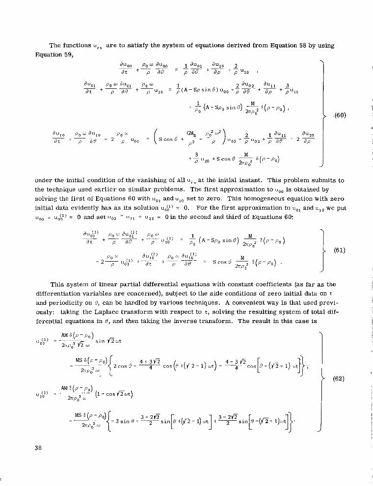
The functions urs are to satisfy the system of equations derived from Equation 58 by using Equation 59,

+ - ( A - s ~ , s ine ) - ~ ( p - p , ) , 1 M PO 2np:

f p u z O 3 + S c o s B 2 M q P - P , )

%Po J under the initial condition of the vanishing of all urs at the initial instant. This problem submits to the technique used earlier on similar problems. The first approximation to uoo is obtained by solving the first of Equations 60 with uo l and u l 0 se t to zero. This homogeneous equation with zero initial data evidently has as its solution u::) = 0. For the first approximation to uO1 and u l 0 we put uo0 = u,,$$) = 0 and set uoz u l l = u z 0 = 0 in the second and third of Equations 60:

This system of linear partial differential equations with constant coefficients (as far as the differentiation variables a r e concerned), subject to the side conditions of zero initial data on t

and periodicity on e, can be handled by various techniques. A convenient way is that used previously: taking the Laplace transform with respect to t, solving the resulting system of total differential equations in 8 , and then taking the inverse transform. The result in this case is

38

I

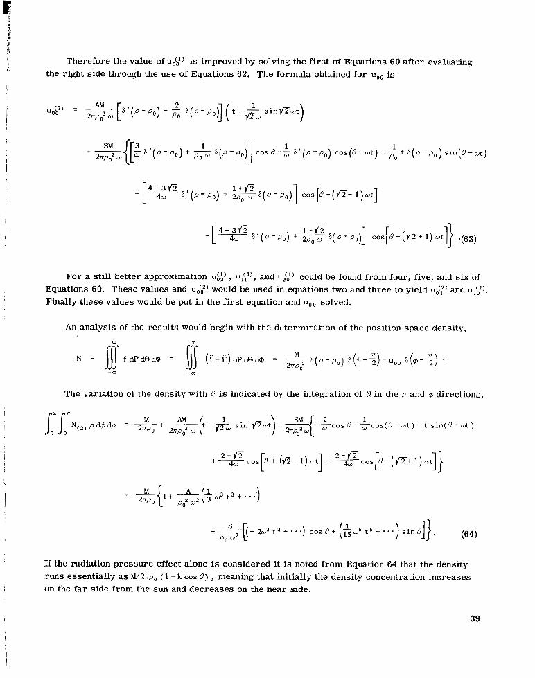
Therefore the value of u i k ) is improved by solving the first of Equations 60 after evaluating the right side through the use of Equations 62. The formula obtained for uoo is

- - 4 + 3 G 1 + f i [ 4w q P - P , ) + - s ( P - P o ) ] c o s p + ( f i - l ) w t ]

For a still better approximation ubi), uiI1), and "2:) could be found from four, five, and six of Equations 60. These values and u&;) would be used in equations two and three to yield ud:) and u::). Finally these values would be put in the first equation and u o o solved.

An analysis of the results would begin with the determination of the position space density,

N = 11 f dPdOdQ = 111 ( P + F ) d P d O d Q = 2.rpoz 6 ( p - p o ) F ( + - $ ) t u O O Z(4-5) . M

- m -m

The variation of the density with e is indicated by the integration of N in the p and 4 directions,

If the radiation pressure effect alone is considered it is noted from Equation 64 that the density runs essentially as M/2npO (1 - k COS S ) , meaning that initially the density concentration increases on the far side from the sun and decreases on the near side.

39

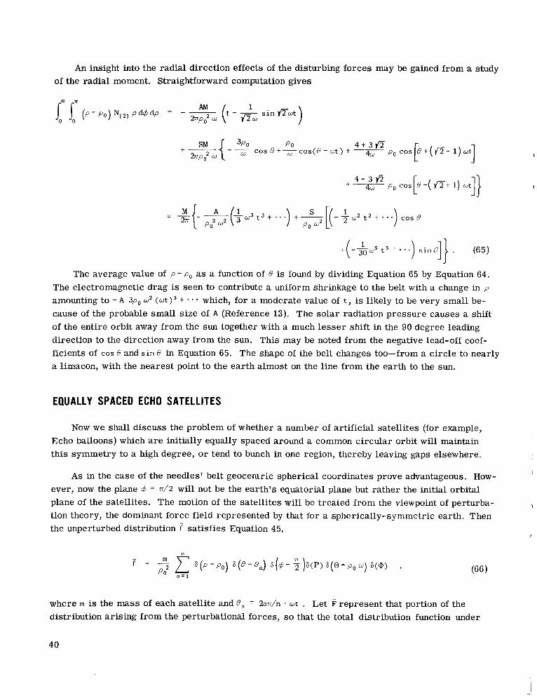
An insight into the radial direction effects of the disturbing forces may be gained from a study of the radial moment. Straightforward computation gives

The average value of P - po as a function of e is found by dividing Equation 65 by Equation 64. The electromagnetic drag is seen to contribute a uniform shrinkage to the belt with a change in p

amounting to - A 3p, u2 (ut )3 t * * . which, for a moderate value of t , is likely to be very small because of the probable small size of A (Reference 13). The solar radiation pressure causes a shift of the entire orbit away from the sun together with a much lesser shift in the 90 degree leading direction to the direction away from the sun. This may be noted from the negative lead-off coefficients of C O S 0 and s i n 0 in Equation 65. The shape of the belt changes too-from a circle to nearly a limacon, with the nearest point to the earth almost on the line from the earth to the sun.

EQUALLY SPACED ECHO SATELLITES

Now we shall discuss the problem of whether a number of artificial satellites (for example, Echo balloons) which are initially equally spaced around a common circular orbit will maintain this symmetry to a high degree, or tend to bunch in one region, thereby leaving gaps elsewhere.

As in the case of the needles' belt geocentric spherical coordinates prove advantageous. How- ever, now the plane 4 = d 2 will not be the earth's equatorial plane but rather the initial orbital plane of the satellites. The motion of the satellites will be treated from the viewpoint of perturba- !

tion theory, the dominant force field represented by that for a spherically-symmetric earth. Then the unperturbed distribution satisfies Equation 45, ,

where m is the mass of each satellite and = 2a~/n t w t . Let represent that portion of the distribution arising from the perturbational forces, so that the total distribution function under

40

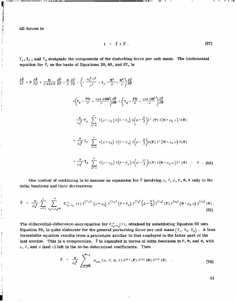
all forces is

T,, To , and Tb designate the components of the disturbing force per unit mass. The fundamental equation for g, on the basis of Equations 39, 66, and 67, is

n

+ 7 T S ( p - p o ) S ( 8 - B a ) S 6' (P) S ( O - p , w ) S ( @ ) m

Po a= 1

One method of continuing is to assume an expansion for f involving P , 8 , 4 , P, 0, @ Only in the delta functions and their derivatives:

m

The differential-difference-sum equation for C.",-..,'t ), obtained by substituting Equation 69 into Equation 68, is quite elaborate for the general perturbing force per unit mass (T,, T,, T+) . A less formidable equation results from a procedure similar to that employed in the latter part of the last section. This is a compromise. e is expanded in te rms of delta functions in P, 0, and @, with p , 8 , and 4 (and t ) left in the to-be-determined coefficients. Then

4 1

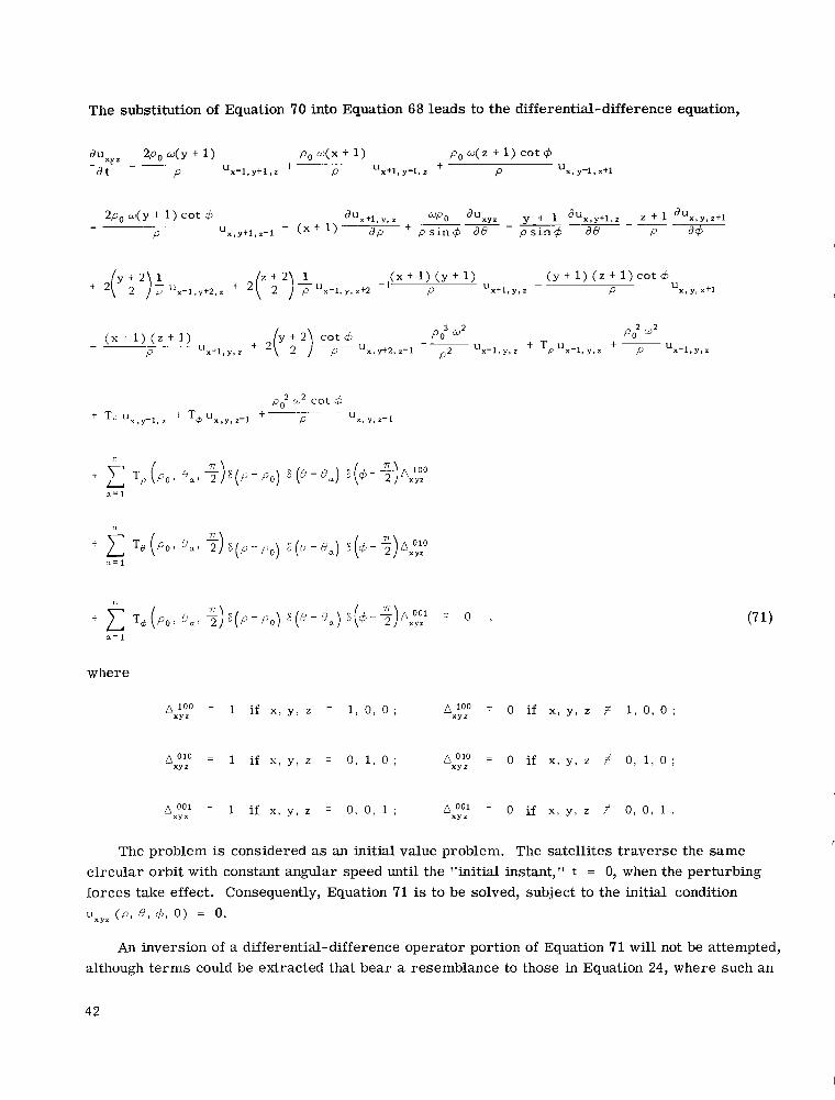
The substitution of Equation 70 into Equation 68 leads to the differential-difference equation,

duxyz 2Po 4 Y f 1) Po 4 x f 1) p o w ( z t l ) c o t + "

d t P U x - l , y + l , z P U X+l, y-1. z P u x , y-1, z+1 t t

+ 2(y 1 2): U x - l , y t z , r + 2 i" 1 2, + U x - L y . z+z - ' (x 1) (Y 1) ( y t 1) ( z t 1) cot $6 P

- U X t l , Y , Z P u x . Y. Z + l

The problem is considered as an initial value problem. The satellites traverse the same circular orbit with constant angular speed until the "initial instant," t = 0, when the perturbing forces take effect. Consequently, Equation 71 is to be solved, subject to the initial condition

UXYZ (Q, 8, d , 0 ) = 0.

An inversion of a differential-difference operator portion of Equation 71 will not be attempted, although terms could be extracted that bear a resemblance to those in Equation 24, where such an

42

1 1 1

1 inversion was accomplished. Nor shall we be satisfied with merely inverting d/d t . Rather, a technique will be used that lies between these extremes. The difference operator aspect will be treated

1

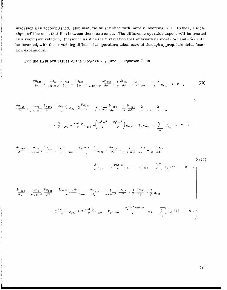
I as a recursion relation. Inasmuch as it is the e variation that interests us most d / d t and d / d e wi l l I be inverted, with the remaining differential operators taken care of through appropriate delta func- I tion expansions.

! For the first few values of the integers X, y, and Z, Equation 71 is

43

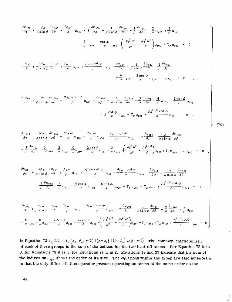
4 -- 3 cot q5 p - ~ p u021 ' Te UOlO = 0 '

2 duo12 4 4 cot q5 6 cot q5 p; w2 cot 4 " -

p dq5 - p u~~~ - ___ p '"012 + ___ p u030 + uOOl + Tq5uO10 ' p UOlO = 0 1

6 6 2 cot q5 2 cot 4 p; a2cotq5 + p u o o 3 - p u z 0 1 -- p '"102 +- p Ul20 UOOl + T, UOOl + T4 UlOO + ~- p UlOO = 0 .

In Equation 73 T 626 = T, ( p o , e,, n / 2 ) 6 ( p - po) 6 (0 - ea) 6 (4 - ~ 1 2 ) . The common characteristic of each of these groups is the sum of the indices for the two lead-off terms. For Equation 72 it is 0, for Equations 73 it is 1, for Equations 74 it is 2. Equations 19 and 37 indicate that the sum of the indices on uxyz shows the order of its size. The equations within any group are also noteworthy in that the only differentiation operator present operating on terms of the same order as the

PO

44

I

1' I, , this operator, recalling that the side conditions a r e that u x Y z = 0 for t = 0 and that uxy, is periodic

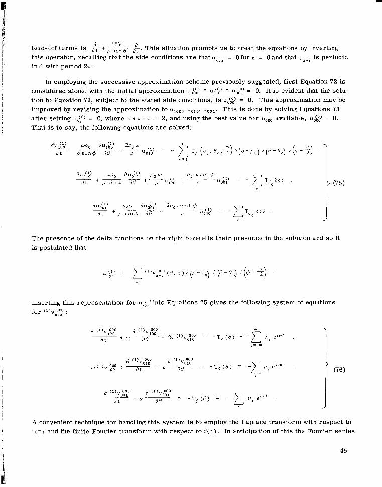
I: In employing the successive approximation scheme previously suggested, first Equation 72 is

lead-off terms is E + a This situation prompts us to treat the equations by inverting

in 8 with period 277.

x. a ii' ;r

i: 1 I

considered alone, with the initial approximation ui&) = u,,(po' = uo6",' = 0. It is evident that the solu- 1 I

tion to Equation 72, subject to the stated side conditions, is ui$ = 0. This approximation may be

after setting = 0, where X t y t z = 2, and using the best value for uooo available, u,,($,) = 0. That is to say, the following equations a r e solved:

4 improved by revising the approximation to u l o 0 , uo l0 , uOo1. This is done by solving Equations 73

J The presence of the delta functions on the right foretells their presence in the solution and so it is postulated that

Inserting this representation for u:;; into Equations 75 gives the following system of equations for ( l ) v 0 0 0 .

x y z .

A convenient technique for handling this system is to employ the Laplace transform with respect to t ( - ) and the finite Fourier transform with respect to e(.'-). In anticipation of this the Fourier series

I a 45

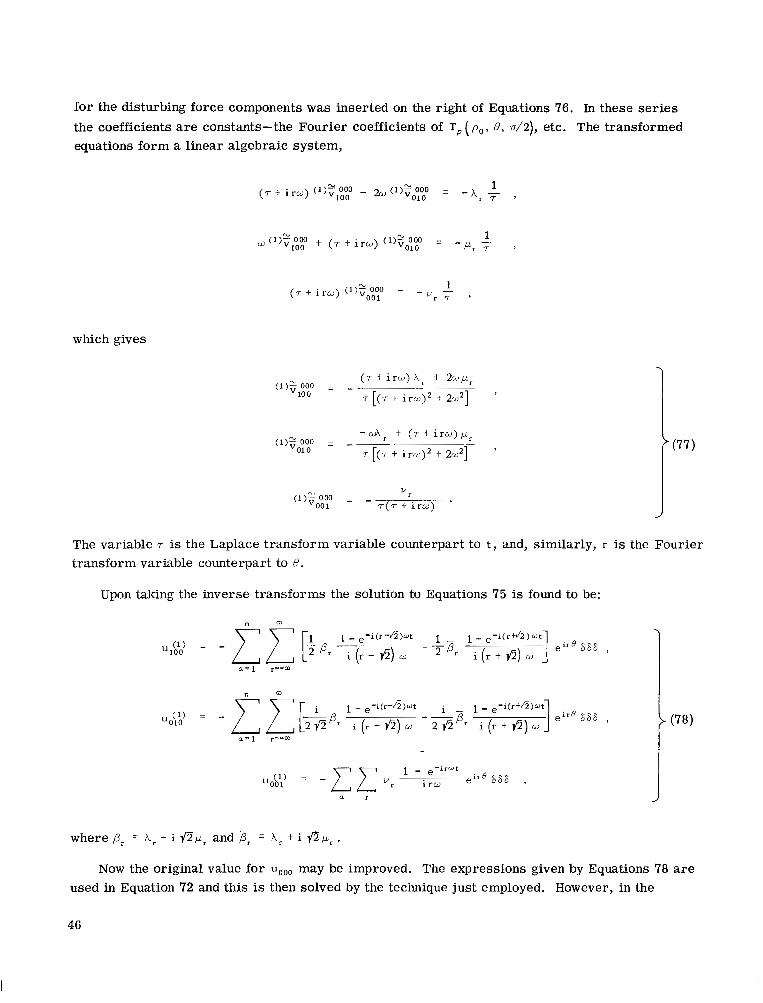
for the disturbing force components was inserted on the right of Equations 76. In these series the coefficients are constants-the Fourier coefficients of T, ( p o , 8 , d 2 ) , etc. The transformed equations form a linear algebraic system,

which gives

(1): 000 = - u r 00 1 7 ( 7 + i r o )

The variable 7 is the Laplace transform variable counterpart to t , and, similarly, r is the Fourier transform variable counterpart to 8.

Upon taking the inverse transforms the solution to Equations 75 is found to be:

a r J Now the original value for uooo may be improved. The expressions given by Equations 78 a r e

used in Equation 72 and this is then solved by the technique just employed. However, in the

46

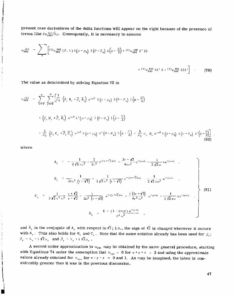
I

present case derivatives of the delta functions will appear on the right because of the presence of terms like du:ob)/ap. Consequently, it is necessary to assume

The value as determined by solving Equation 72 is

where

A second order approximation to uooo may be obtained by the same general procedure, starting with Equations 74 under the assumption that uxyz = 0 for x + Y + z = 3 and using the approximate values already obtained for uxyl for x + Y + z = 0 and 1. As may be imagined, the labor is considerably greater than it was in the previous discussion.

47

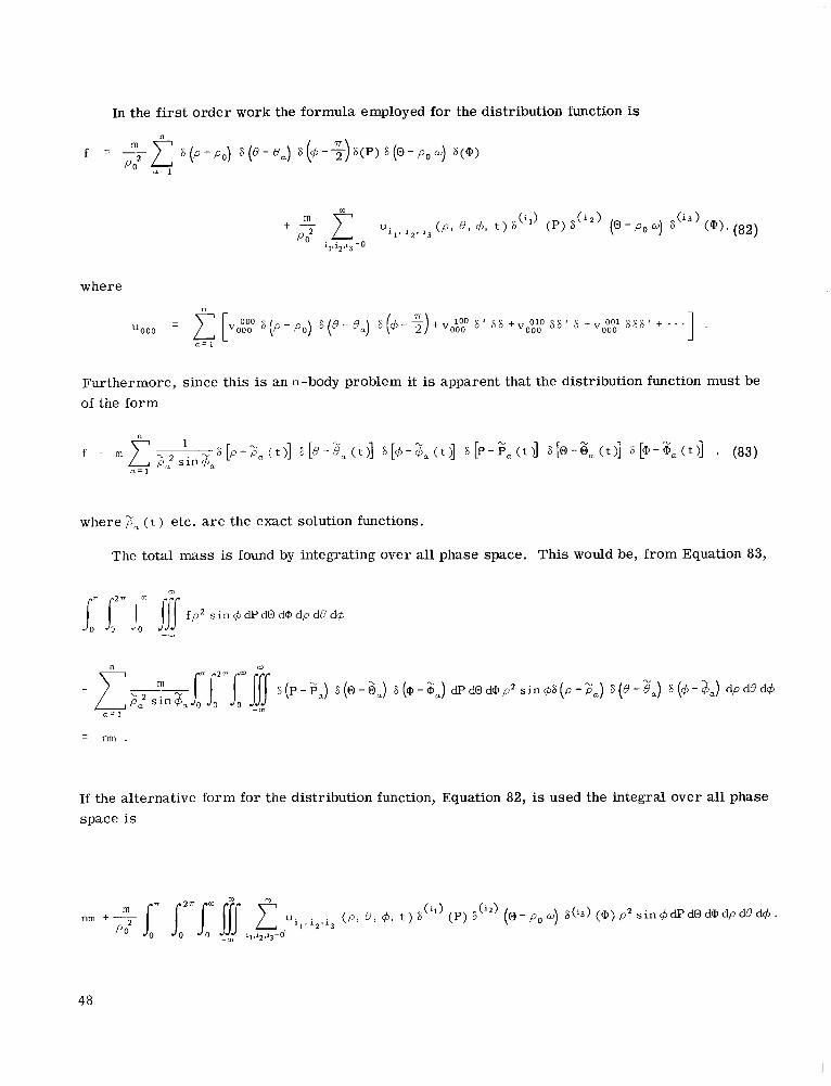
In the first order work the formula employed for the distribution function is

" i i L = o 1' 2' 3

where

Furthermore, since this is an n-body problem it is apparent that the distribution function must be of the form

where i;, ( t ) etc. are the exact solution functions.

The total mass is found by integrating over all phase space. This would be, from Equation 83,

If the alternative form for the distribution function, Equation 82, is used the integral over all phase space is

48

(1

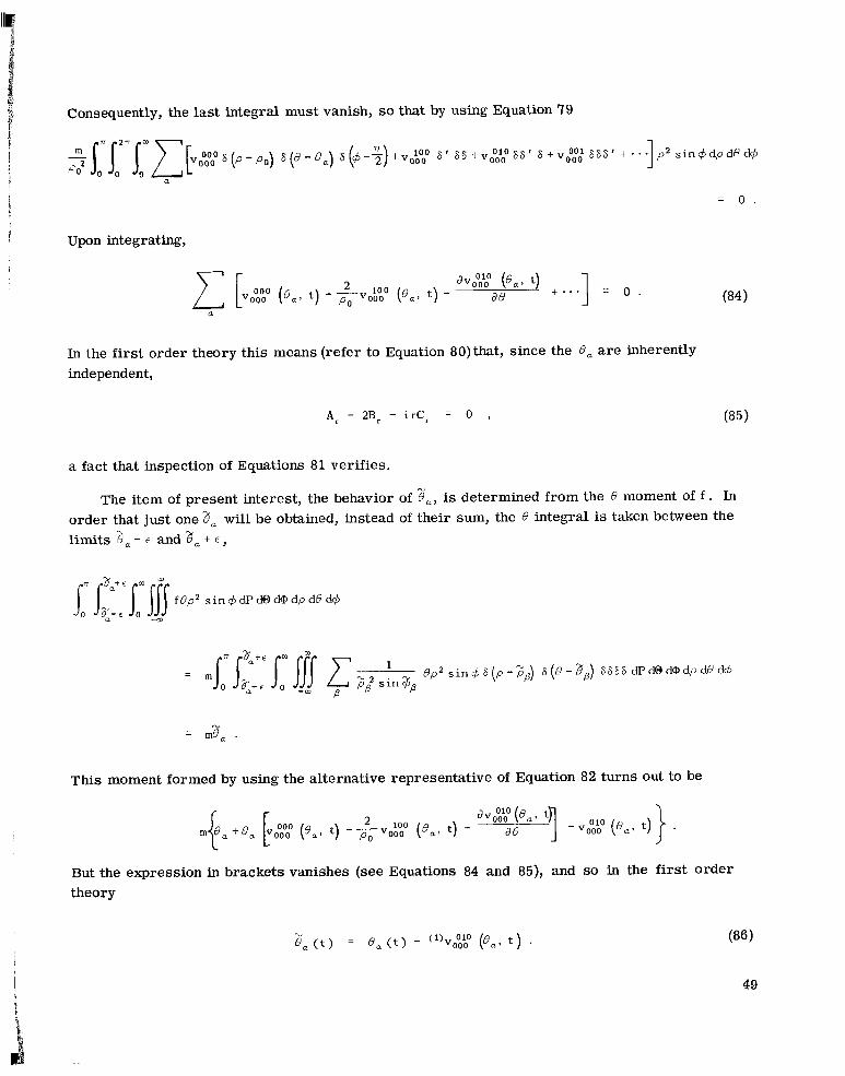
= 0 .

Upon integrating,

In the first order independent,

theory this means (refer to Equation 80) that, since the ea a r e inherently

Ar - 2Br - i r C r = 0 ,

a fact that inspection of Equations 81 verifies.

This moment formed by using the alternative representative of Equation 82 turns out to be

But the expression in brackets vanishes (see Equations 84 and 85), and so in the first order theory

49

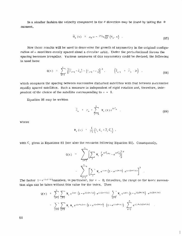
In a similar fashion the velocity component in the B direction may be found by taking the 0 moment,

Now these results will be used to determine the growth of asymmetry in the original configuration of n satellites evenly spaced about a circular orbit. Under the perturbational forces the spacing becomes irregular. Various measures of this asymmetry could be devised; the following is used here:

which compares the spacing between successive disturbed satellites with that between successive equally spaced satellites. Such a measure is independent of rigid rotation and, therefore, independent of the choice of the satellite corresponding to a = 1.

Equation 86 may be written

where

w r ( t ) = (2. cr + E , C') ?

1

with Cr given in Equations 81 (see also the remarks following Equation 81). Consequently,

50

i 4

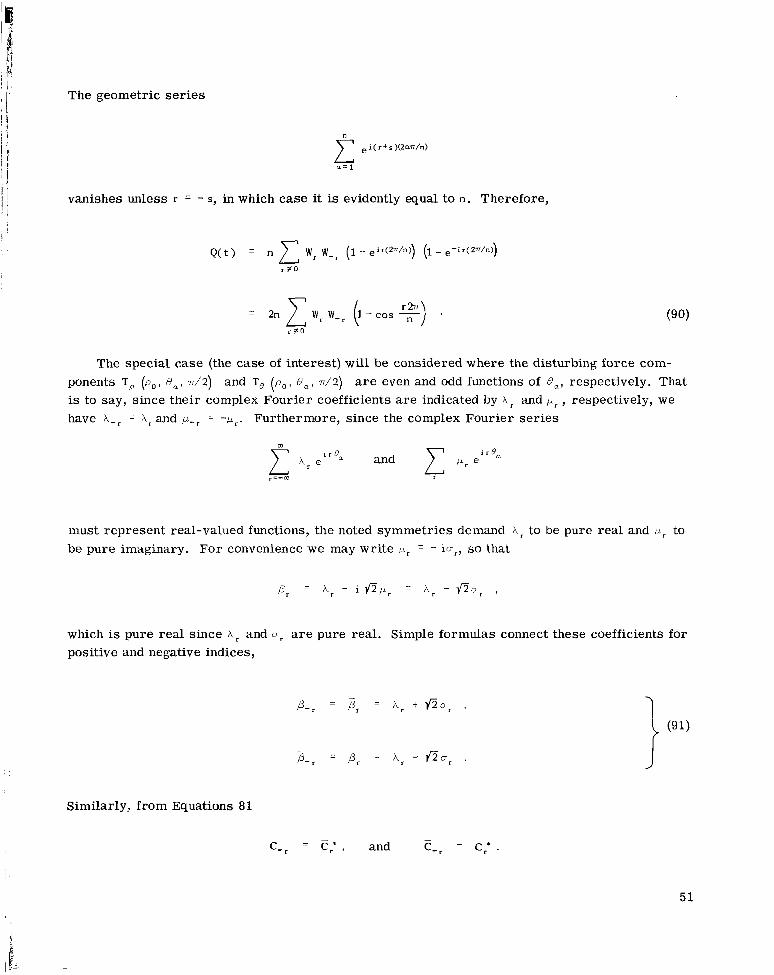
I I!' The geometric series

i / 1 1

The special case (the case of interest) will be considered where the disturbing force components T, (po , e a , d 2 ) and T, (p,, , ea, d 2 ) a r e even and odd functions of B a , respectively. That is to say, since their complex Fourier coefficients are indicated by A r and pr , respectively, we have A_, = A r and p-r -p,. Furthermore, since the complex Fourier series

must represent real-valued functions, the noted symmetries demand h r to be pure real and p, to be pure imaginary. For convenience we may write I", = - i m r , so that

which is pure real since X r and ur are pure real . Simple formulas connect these coefficients for positive and negative indices,

Similarly, from Equations 81

C-r = C,* , and - -

C r = c,' .

51

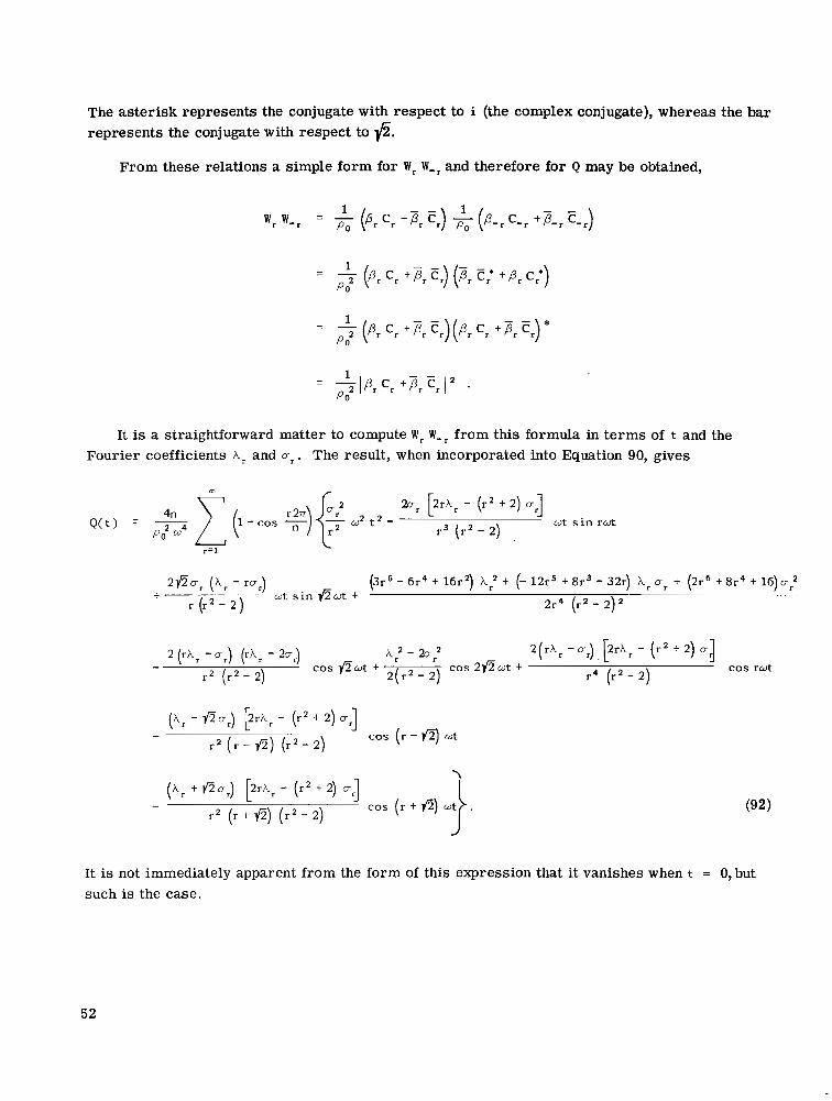
The asterisk represents the conjugate with respect to i (the complex conjugate), whereas the bar represents the conjugate with respect to fi.

From these relations a simple form for Wr W,, and therefore for Q may be obtained,

It is a straightforward matter to compute W r W - r from this formula in terms of t and the Fourier coefficients X r and my. The result, when incorporated into Equation 90, gives

2 f i 5 (h. - r q , (3r6 - 6r4 t 16r') h: t (- 12r5 + 8 r 3 - 32r) X r or + (2r6 t 8r4 t 1 6 ) ~ : t" w t s i n f i w t +

r (r' - 2 ) - . ~

2r4 (r' - 2)'

2 (rh, -or) (rh, - 254 A; - 2Cr; 2(rXr -mr).[2rAr - ( r ' t 2 ) ~4 r' (r' - 2)

cos f i w t f cos 2 f i w t + 2 ( r' - 2) r4 [r'- 2)

cos rut

( A r - f i m r ) [2rhr - (r' + 2) .-.I -

r z ( r - e) ( r 2 - 2) cos (r - fi) w t

It is not immediately apparent from the form of this expression that it vanishes when t = 0, but such is the case.

52

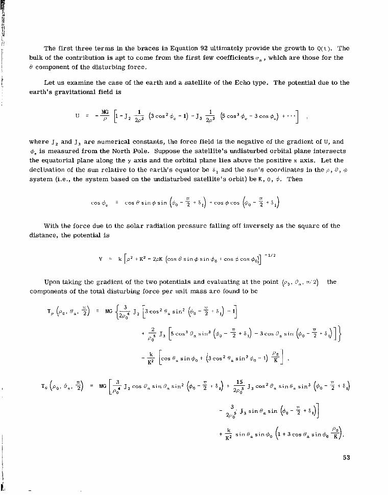
The first three terms in the braces in Equation 92 ultimately provide the growth to Q(t). The bulk of the contribution is apt to come from the first few coefficients vn, which are those for the 8 component of the disturbing force.

Let us examine the case of the earth and a satellite of the Echo type. The potential due to the earth's gravitational field is

where J 2 and J 3 are numerical constants, the force field is the negative of the gradient of U, and +e is measured from the North Pole. Suppose the satellite's undisturbed orbital plane intersects the equatorial plane along the y axis and the orbital plane lies above the positive X axis. Let the declination of the sun relative to the earth's equator be 8, and the sun's coordinates in the p , 8 , 4 system (i.e., the system based on the undisturbed satellite's orbit) be K , 0, 4. Then

With the force due to the solar radiation pressure falling off inversely as the square of the distance, the potential is

V = k [p2 + K Z - 2pK (cos 8 s i n 4 s i n 4o f cos 4 cos do)] - 1 / 2

Upon taking the gradient of the two potentials and evaluating at the point (po , Q a , n / ' 2 ) the components of the total disturbing force per unit mass a r e found to be

+ po5 J 3

- - cos ea s i n 4 0 + (3 cos2 ea - 1) $1 ,

2 [5 cos3 8, s i n 3 (&o - 3 f S1) - 3 c o s 8 , s i n (do - 5 f S3]} 77

" [ P

K*

+ - s i n B , s i n 4 0 k

K2

53

1 + 3 cos Ba s i n do

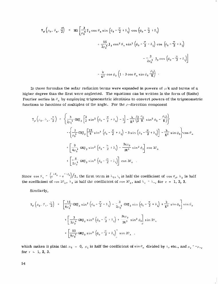
In these formulas the solar radiation terms were expanded in powers of p / K and terms of a higher degree than the first were neglected. The equations can be written in the form of (finite) Fourier series in B a by employing trigonometric identities to convert powers of the trigonometric functions to functions of multiples of the angle. For the p-direction component

+{$mJ3psin3 (+o-T 77 + E l ) - 3 ~ i n ( + ~ - + t S ~ ) ] - k

Similarly,

t r-GMJ, 15 s i n 3 (do - 5 + sl)] s i n , L@,S

which makes it plain that po = 0, p l is half the coefficient of s i n Ba divided by i , etc., and pr = - P - ~

for r = 1, 2, 3.

54

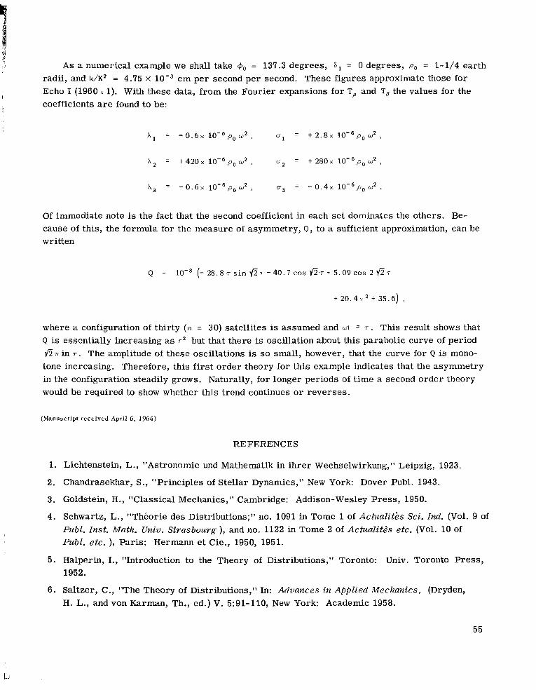
t: As a numerical example we shall take $o = 137.3 degrees, 6, = 0 degrees, po = 1-1/4 earth radii, and k/K' = 4.75 X l o e 3 cm per second per second. These figures approximate those for Echo I (1960 L 1). With these data, from the Fourier expansions for T, and T, the values for the

I I coefficients are found to be:

~

A , = - 0 . 6 ~ 10-6po u' , m1 = + 2 . 8 ~ 1 0 - 6 p o w ' ,

A, = + 4 2 0 x 1 0 - 6 p o u ' , mz = t 280x po w 2 ,

A, = - 0 . 6 ~ 1 0 - 6 p o u ' , o3 = - 0 . 4 x 10-6pow'

+ 2 0 . 4 7 ' + 3 5 . 6 ) ,

where a configuration of thirty (n = 30) satellites is assumed and w t r . This result shows that Q is essentially increasing as r' but that there is oscillation about this parabolic curve of period f i n in r . The amplitude of these oscillations is so small, however, that the curve for Q is mono- tone increasing. Therefore, this first order theory for this example indicates that the asymmetry in the configuration steadily grows. Naturally, for longer periods of time a second order theory would be required to show whether this trend continues o r reverses.

(Manuscript received April 6, 1964)

REFERENCES

1. Lichtenstein, L., "Astronomie und Mathematik in ihrer Wechselwirkung,T' Leipzig, 1923.

2 . Chandrasekhar, S., "Principles of Stellar Dynamics," New York: Dover Publ. 1943.

3. Goldstein, H., "Classical Mechanics," Cambridge: Addison-Wesley Press, 1950.

4 . Schwartz, L., "Theorie des Distributions;'' no. 1091 in Tome 1 of Actualit& Sci. I d . (Vol. 9 of Publ. Inst. Math. Univ. Strasbourg ), and no. 1122 in Tome 2 of Actualitds etc. (Vol. 10 of Publ. etc. ), Paris: Hermann et Cie., 1950, 1951.

5 . HalPerb, I., "Introduction to the Theory of Distributions," Toronto: Univ. Toronto Press, 1952.

6 . Saltzer, C., "The Theory of Distributions,'' In: Advances in Applied Mechanics, (Dryden, H. L., and von Karman, Th., ed.) V. 5:91-110, New York: Academic 1958.

55

7. Courant, R., and Hilbert, D., "Methoden de r Mathematischen Physik," Berlin: J. Springer, 1937.

8. Milne-Thomson, L. M., "The Calculus of Finite Differences," Macmillan: London, 1960.

9. Goldberg, L., "Project West Ford-Properties and Analyses. Introduction," Astronom. J. 66(3):105-106, April 1961.

10. Morrow, W. E., Jr., and MacLellan, D. C., "Properties of Orbiting Dipole Belts," Astronom. J. 66(3):107-113, April 1961.

11. Liller, W., "Report on the Effects of Project West Ford on Optical Astronomy," Astronom. J. 66(3):114-116, April 1961.

12. Lilley, A. E., "Radio Properties of an Orbiting Scattering Medium," Astronom. J. 66(3):116- 118, April 1961.

13. Singer, S. F., "Interaction of West Ford Needles with Earth's Magnetosphere," Nature 192:303- 306, October 28, 1961.

14. Friedman, B., "Principles and Techniques of Applied Mathematics," New York Wiley, 1956.

56 NASA-Langley, 1965 G- 57 5

“The aeronautical and space activities of the United States shall be conducted so as to contribute . . . to the expansion of human knowledge of phenomena in the atmosphere and space. The Administration shall provide for the widest practicable and appropriate dissemination of information concerning its activities and the results thereof.”

“ N A T l O N A L AERONAUTICS AND SPACE ACT OF 1958

NASA SCIENTIFIC AND TECHNICAL PUBLICATIONS

TECHNICAL REPORTS: Scientific and technical information considered important, complete, and a lasting contribution to existing knowledge.

TECHNICAL NOTES: Information less broad in scope but nevertheless of importance as a contribution to existing knowledge.

TECHNICAL MEMORANDUMS: Information receiving limited distribution because of preliminary data, security classification, or other reasons.

CONTRACTOR REPORTS: Technical information generated in con- nection with a NASA contract or grant and released under NASA auspices.

TECHNICAL TRANSLATIONS: Information published in a foreign language considered to merit NASA distribution in English.

TECHNICAL REPRINTS: Information derived from NASA activities and initially published in the form of journal articles.

SPECIAL PUBLICATIONS Information derived from or of value to NASA activities but not necessarily reporting the results .of individual NASA-programmed scientific efforts. Publications include conference proceedings, monographs, data compilations, handbooks, sourcebooks, and special bibliographies.

Details on the availability of these publications may be obtained horn:

SCIENTIFIC AND TECHNICAL INFORMATION DIVISION

NATIONAL AERONAUTICS AND SPACE ADMINISTRATION

Washington, D.C. PO546

LIOUVILLE'S EQUATION AND THE n-BODY PROBLEM

Documents

Transcript of LIOUVILLE'S EQUATION AND THE n-BODY PROBLEM