#15: Final Project: Roller Coaster! CSE167: Computer Graphics Instructor: Ronen Barzel UCSD, Winter...

#15: Final Project: Roller Coaster!

CSE167: Computer GraphicsInstructor: Ronen Barzel

UCSD, Winter 2006

2

QuickTime™ and aTIFF (Uncompressed) decompressor

are needed to see this picture.




are needed to see this picture. QuickTime™ and aTIFF (Uncompressed) decompressor








Roller coasters…

3

Final project

Build a roller coaster, with a car riding on it

More open-ended than previous projects

Be creative! We do have some specific capabilities/features we’ll look for

But we’ll be impressed by “style” too!

4

Final project

More on your own than previous projects No “base code”

though you may use base code from previous assignments

Today I’ll go over the key techniques

5

Roller coaster steps

(see web page for details)1. Make a piecewise-cubic curve 2. Create coordinate frames along a

piecewise-cubic curve will be used to orient along the path include a roll angle at each curve point, to

adjust tilt

3. Create a swept surface the actual track along the of the roller

coaster

4. Design and build the roller coaster track5. Run a car on the track

6

Step 1. Piecewise-Cubic Curve

Specify as a series of points Will be used for the path of the roller coaster

QuickTime™ and aTIFF (LZW) decompressor


7

Step 2. Coordinate Frames on curve

Describes orientation along the path



8

Step 2b. Tweak coordinate frames

Control lean of coordinate frames Specify “roll” angle offset at each control point



9

Step 3a. Sweep a cross section

Define a cross section curve (piecewise-linear is OK)

Sweep it along the path, using the frames



10

3b. Tessellate

Construct triangles using the swept points (sweep more finely than this drawing, so it’ll be smoother)



11

4. Run a car on the track



12

Step 1. Piecewise-Cubic Curve

Specify as a series of points Will be used for the path of the roller coaster



13

Piecewise-Cubic Curve

Requirements: Given an array of N points Be able to evaluate curve for any value of t (in 0…1)

Curve should be C1-continuous

Best approach: define a class, something like

class Curve {Curve(int Npoints, Point3 points[]);Point3 Eval(float t);

}

14

Piecwise-Cubic Curves

Three recommended best choices:

Bézier segments• Advantages: You did a Bézier segment in Project 5• Disadvantages: Some work to get C1 continuity

• Will discuss technique to do this

B-Spline• Advantages: simple, always C1 continuous• Disadvantages: New thing to implement, doesn’t interpolate

Catmull-Rom spline• Advantages: interpolates points• Disadvantages: Less predictable than B-Spline. New thing to implement

15

Piecewise Bézier curve review

We have a Bézier segment function Bez(t,p0,p1,p2,p3) Given four points Evaluates a Bézier segment for t in 0…1 Implemented in Project 5

Now define a piecewise Bézier curve x(u) Given 3N+1 points p0,… p3N

Evaluates entire curve for u in 0…1 Note: In class 8, defined curve for u in 0…N

• Today will define it for u in 0…1

16

Piecewise Bézier curve: segments

• Given 3N +1 points p0 ,p1,K ,p3N

• Define N Bézier segments :

x0 (t) = Bez(t,p0 ,p1,p2 ,p3)

x1(t) = Bez(t,p3,p4 ,p5 ,p6 )

M

xN −1(t) = Bez(t,p3N −3,p3N −2 ,p3N −1,p3N )

x0(t)

x1(t)

x2(t)

x3(t)

p0

p1p2

p3

p4p5

p6

p7 p8

p9

p10 p11

p12

17

Piecewise Bézier curve

x0(t)

x1(t)

x2(t)

x3(t)

x(0.3)

x(0.71)

x(0.25)x(0.0)

x(0.5) x(0.75)

x(1.0)

x(u) =

x0 (Nu), 0 ≤u≤ 1N

x1(Nu−1), 1N ≤u≤ 2

N

M M

xN−1(Nu−(N −1)), N−1N ≤u≤1

⎧

⎨⎪⎪

⎩⎪⎪

x(u) =xi Nu−i( ), where i = Nu⎢⎣ ⎥⎦,u <1;

= Bez(Nu − i,p3i ,p3i+1,p3i+2,p3i+3)

x(1) = p3N

= Bez(1,p3i ,p3i+1,p3i+2,p3i+3)

18

Piecewise Bézier curve

3N+1 points define N Bézier segments x(i/N)=p3i

C0 continuous by construction G1 continuous at p3i when p3i-1, p3i, p3i+1 are collinear

C1 continuous at p3i when p3i-p3i-1 = p3i+1-p3i

p0

p0

p1

p2

P3

P3

p2

p1

p4

p5

p6

p6

p5

p4

C1 continuousC1 discontinuous

19

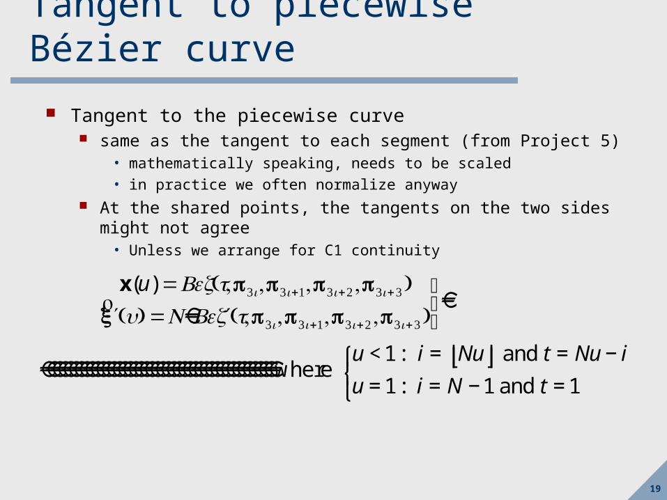
Tangent to piecewise Bézier curve

Tangent to the piecewise curve same as the tangent to each segment (from Project 5)

• mathematically speaking, needs to be scaled• in practice we often normalize anyway

At the shared points, the tangents on the two sides might not agree• Unless we arrange for C1 continuity

x(u) =Bez(t,p3i ,p3i+1,p3i+2 ,p3i+3)′

rx (u) =N Be ′z (t,p3i ,p3i+1,p3i+2 ,p3i+3)

⎫⎬⎭

where u <1: i = Nu⎢⎣ ⎥⎦ and t = Nu− i

u = 1: i = N −1 and t = 1

⎧⎨⎩

20

Piecewise Bézier curves

Inconveniences: Must have 4 or 7 or 10 or 13 or … (1 plus a multiple

of 3) points Not all points are the same Have to fiddle to keep curve C1-continuous

21

Making a C1 Bézier curve

A hack to construct a C1-continuous Bézier curve Actually, this is essentially implementing Catmull-Rom splines

Instead, could just implement Catmull-Rom splines directly• Same amount of work as implementing B-Spline

Given M points: want a piecewise-Bézier curve that interpolates them

Bézier segments interpolate their endpoints Need to construct the intermediate points for the segments



22

Auto-creation of intermediate points

Given M original points Will have M-1 segments Will have N=3*(M-1)+1 final points



23




Need tangent directions at each original point Use direction from previous point to next point

24




Introduce intermediate points Move off each original point in the direction of the tangent

“Handle” length = 1/3 distance between previous and next points

special-case the end segments. • or for closed loop curve, wrap around

25




Resulting curve:

26


Summary of algorithm:Given M originalPointsAllocate newPoints array, N = 3*(M-1)+1 new pointsfor each original point i p = originalPoints[i] v = originalPoints[i+1]-originalPoints[i-1] newPoints[3*i-1] = p-v/6 newPoints[3*i] = p newPoints[3*i-1] = p+v/6

Of course, must be careful about start and end of loop

Can allow the curve to be a closed loop: wrap around the ends

27

Other option… B-spline

Need at least 4 points, i.e. N+3 points B-spline curve uses given N+3 points as is

Always C2 continuous• no intermediate points needed

Approximates rather than interpolates• doesn’t reach the endpoints• not a problem for closed loops: wrap around.

simple algorithm to compute• (may need to extend matrix library to support Vector4)

28

Evaluate Bézier using “Sliding window”

Window moves forward by 3 units when u passes to next Bézier segment

With 3N+1 points, N positions for window, ie. N segments Evaluate matrix in window:

Blending Functions Review



x(u) = p3i p3i+1 p3i+2 p3i+3[ ]

GBez

1 24 4 44 34 4 4 4

−1 3 −3 13 −6 3 0−3 3 0 01 0 0 0

⎡

⎣

⎢⎢⎢⎢

⎤

⎦

⎥⎥⎥⎥

BBez

1 24 4 34 4

t3

t2

t1

⎡

⎣

⎢⎢⎢⎢

⎤

⎦

⎥⎥⎥⎥

T{

where u <1: i = Nu⎢⎣ ⎥⎦ and t = Nu− i

u = 1: i = N −1 and t = 1

⎧⎨⎩

29

B-spline blending functions

Still a sliding “window” Shift “window” by 1, not by 3 With N+3 points, N positions for window, i.e. N segments





x(u) = pi pi+1 pi+2 pi+3[ ]

G1 24 4 4 34 4 4

16

−1 3 −3 13 −6 0 4−3 3 3 11 0 0 0

⎡

⎣

⎢⎢⎢⎢

⎤

⎦

⎥⎥⎥⎥

BB−spline

1 24 44 34 4 4

t3

t2

t1

⎡

⎣

⎢⎢⎢⎢

⎤

⎦

⎥⎥⎥⎥

T{

where u <1: i = Nu⎢⎣ ⎥⎦ and t = Nu − i

u = 1: i = N −1 and t = 1

⎧⎨⎩

30

Tangent to B-spline

Same formulation, but use T’ vector (and scale by N)

x(u) = pi pi+1 pi+2 pi+3[ ]

G1 24 4 4 34 4 4

16

−1 3 −3 13 −6 0 4−3 3 3 11 0 0 0

⎡

⎣

⎢⎢⎢⎢

⎤

⎦

⎥⎥⎥⎥

BB−spline

1 24 44 34 4 4

t3

t2

t1

⎡

⎣

⎢⎢⎢⎢

⎤

⎦

⎥⎥⎥⎥

T{


u = 1: i = N −1 and t = 1

⎧⎨⎩

′rx (u) = pi pi +1 pi +2 pi +3[ ]

G1 24 4 4 34 4 4

1

6

−1 3 −3 1

3 −6 0 4

−3 3 3 1

1 0 0 0

⎡

⎣

⎢⎢⎢⎢

⎤

⎦

⎥⎥⎥⎥

BB−spline

1 24 44 34 4 4

N

3t 2

2t

1

0

⎡

⎣

⎢⎢⎢⎢

⎤

⎦

⎥⎥⎥⎥

′T{


u = 1: i = N −1 and t = 1

⎧⎨⎩

31

Catmull-Rom

Use same formulation as B-spline But a different basis matrix

Interpolates all its control points Except it doesn’t reach the endpoints Add extra points on the ends, or wrap around for closed loop

x(u) = pi pi+1 pi+2 pi+3[ ]

G1 24 4 4 34 4 4

12

−1 2 −1 03 −5 0 2−3 4 1 01 −1 0 0

⎡

⎣

⎢⎢⎢⎢

⎤

⎦

⎥⎥⎥⎥

BCatmull−Rom

1 24 44 34 4 4

t3

t2

t1

⎡

⎣

⎢⎢⎢⎢

⎤

⎦

⎥⎥⎥⎥

T{


u = 1: i = N −1 and t = 1

⎧⎨⎩

′rx (u) = pi pi +1 pi +2 pi +3[ ]

G1 24 4 4 34 4 4

1

2

−1 2 −1 0

3 −5 0 2

−3 4 1 0

1 −1 0 0

⎡

⎣

⎢⎢⎢⎢

⎤

⎦

⎥⎥⎥⎥

BCatmull −Rom1 24 44 34 4 4

N

3t 2

2t

1

0

⎡

⎣

⎢⎢⎢⎢

⎤

⎦

⎥⎥⎥⎥

′T{


u = 1: i = N −1 and t = 1

⎧⎨⎩

32

Step 1, Summary

We can define a curve: Given N points We know how to evaluate the curve for any u in 0..1

We know how to evaluate the tangent for any u in 0..1

Might be implemented via Bézier, B-Spline, Catrom

Bundle in a classclass Curve {

Curve(int Npoints, Point3 points[]);Point3 Eval(float u);

Vector3 Tangent(float u);}

33

Step 2. Coordinate Frames on curve

Describes orientation along the path



34

Finding coordinate frames

To be able to build the track, we need to define coordinate frames along the path. We know the tangent, this gives us one axis, the “forward” direction

We need to come up with vectors for the “right” and “up” directions.

There’s no automatic solution Most straightforward :

Use the same approach as camera lookat Pick an “up” vector.

35

Constructing a frame

Same as constructing an object-to-world transfrom

Given that we can compute position x(t) and tangent ′rx (t)

Given a global "up" vector ru

Assume that we want

"forward" direction to be the y axis, "right" to be the x axis

"up" to be the z axis

To construct the frame matrix F(t), fill the ra,

rb,

rc,d columns

d =x(t) -- origin of the frame is at t along the curverb =

′rx (t)′

rx (t)

-- y axis of frame is tangent, normalized

ra=

rb×

ru

rb×

ru

-- x axis of frame is perpendicular to forward and global up

rc=

ra×

rb -- z axis of frame is perpendicular to forward and right

36

Specifying a roll for the frame

The “lookat” method tries to keep the frame upright

But what if we want to lean, e.g. for a banked corner?

Introduce a roll parameter Gives the angle to roll about the “forward” axis.

Want to be able to vary the roll along the path Specify a roll value per control point

37

Computing the roll on the path

How to compute the roll at any value of t? just use the roll values as (1D) spline points!

Given points: p0 ,p1, K , pN−1

and rolls: r0 , r1, K , rN−1

Compute position, tangent:x(u) =Bez(Nu−i,p3i ,p3i+1,p3i+2 ,p3i+3) or

= GiBTNu−ir′x (u) =Be ′z (Nu−i,p3i ,p3i+1,p3i+2 ,p3i+3) or

= GiBN ′TNu−i Compute roll:

r(u) =Bez(Nu−i,r3i ,r3i+1,r3i+2 ,r3i+3) or

= ri ri+1 ri+2 ri+3[ ]BTNu−i

where:

i = Nu⎢⎣ ⎥⎦

38

Rolling the frame

To compute the final object-to-world matrix for the frame, compose the upright frame with a rotation matrix:

W(t) =F(t) R y(r(t))

39

Curve class with frames

The class can include: class Curve {

Curve(int N, Point3 points[], float roll[]); void SetUp(Vector3 up); Point3 Eval(float t); Vector3 Tangent(float t); Matrix Frame(float t) { return UpFrame(t)*Roll(t); }private: Matrix UpFrame(float t); Matrix Roll(float t);}

40

Step 3a. Sweep a cross section

Define a cross section curve (piecewise-linear is OK)

Sweep it along the path, using the frames



41

3b. Tessellate

Construct triangles using the swept points (sweep more finely than this drawing, so it’ll be smoother)



42

The cross section

Say we have a cross section curve with N points AKA the profile curve For simplicity, assume it’s piecewise linear e.g., N=4

q0

q1 q2

q3

43

Sweep the profile curve

choose M how many rows to have make this a parameter or value you can change easily

too few: not smooth enough too many: too slow

place M copies of the cross section along the path e.g. M=8 (for a full track you might have M=100’s or more)

44

Sweep the profile curve

We can get a coordinate frame for any t along the curve i.e. we have an object-to-world matrix W(t) for t in 0…1

Distribute the profile curve copies uniformly in t For each row, transform the profile curve using the world matrix:

For each row i in 0 to M -1

For each profile point q j for j in 0 to N -1

t =i

M −1pij =W(t)qj

45

Topology

Simple rectangular topology, M*N points:



P[iN + j] =W(i (M −1)) qj

46

Putting a car on the track

Again, we can use the path’s frame matrix W(t) Probably with a local offset M if needed:

• Local-to-world = W(t)M

t goes from 0 to 1 and keeps cycling Wheels rotate as function of t

Will probably slide. Try to tweak so they look reasonable.

More complex to really have wheels roll on the track

47

Designing a roller coaster







48

Designing a roller coaster track

Suggestions… plan it out on (graph) paper first!

top view & “unwound” elevation view

number and label the control points• use a scheme that will let you go back and add more points later!

• control point coordinates can be hard-wired in C++ source

• when typing them in, comment them with your labels







49

Designing a roller coaster The path can be fairly simple.

start with something simple if you have time at the end, go wild!

The track could be… a trench, like a log flume that the car slides in a monorail that the car envelops a pair of rails (two cross sections) for a railroad-style

car whatever else you come up with

The car could be… a cube with simple wheels a penguin A sports car that you download off the web and figure out

how to read whatever else you come up with

Trestles/Supports not needed… but could be cool Ticket booth & Flags & Fence etc. not needed… but could

be cool Have fun! Be creative!

50

Advanced Roller Coaster Topics

(Not required, but handy for some bells & whistles)

Arc-Length Parametrization Better control over speed of car

Parallel transport of frames Make it easier to do loops

51

Arc-length Parametrization

In our current formulation: Position along the curve is based on arbitrary t parameter

We animate by increasing t uniformly:• Speed of the car isn’t constant• Speed of the car isn’t easily controllable• Car spends the same amount of time in each segment:

• in areas where the control points are far apart, the car goes fast

• in areas where the control points are close together, the car goes slow

t=0

t=0.1

t=0.2t=0.3

t=0.4

t=0.5

t=0.6

t=0.7

t=0.8 t=0.9

t=1

52

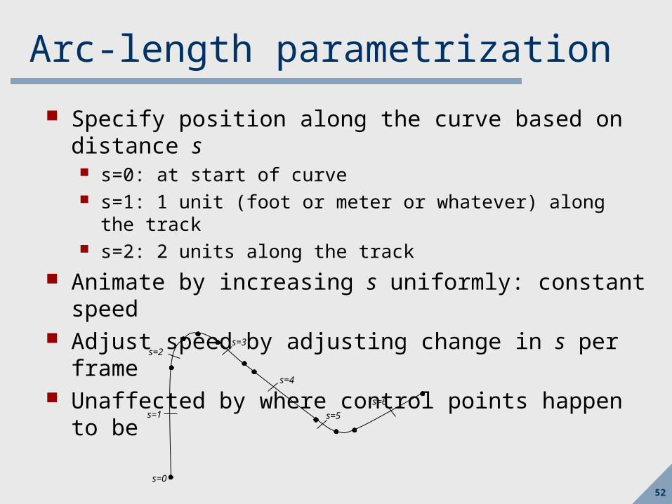
Arc-length parametrization

Specify position along the curve based on distance s s=0: at start of curve s=1: 1 unit (foot or meter or whatever) along the track

s=2: 2 units along the track Animate by increasing s uniformly: constant speed

Adjust speed by adjusting change in s per frame

Unaffected by where control points happen to be

s=0

s=1

s=2s=3

s=4

s=5

s=6

53

Arc-length parametrization

Arc length just means length along the curve

Really, arc length re-parametrization We have a parameter t We want to express t in terms of length s

No simple closed form expression A bit of math in principle Then we’ll do a simple approximation of it

54

Arc length

Define S(t) =length along the curve x(t) from the start until t

ds= dx2 + dy2 + dz2 -- differential distance

S(t) =dsdt

⎛⎝⎜

⎞⎠⎟dt

0

t

∫

=dxdt

⎛⎝⎜

⎞⎠⎟

2

+dydt

⎛⎝⎜

⎞⎠⎟

2

+dzdt

⎛⎝⎜

⎞⎠⎟

2

dt0

t

∫

= ′rx (t)

0

t

∫ dt

55

Reparameterize

We have:

x(t) =our curve parametrized by tS(t) =arc length along x(t) up to t

We want: xarc(s) =our curve re-parametrized by s

xarc(s) =x(t(s)), where t(s) =S−1(s)

We need:

the inverse length function, S−1(s)

56

Arc-length reparameterization

Exact computation of length & inverse is too hard

Simple approximation for arc length: chord length Sample M times, uniformly (sufficiently large, e.g.

M=10N) Accumulate incremental length into array of length

values:

Simple approximation to invert:

Si =Si−1 + x iM( )−x i−1

M( )

Given s, where 0 ≤s≤SM

Find neighboring samples: i such that Si < s< Si+1

Use linear interpolation between the samples:

t =1M

i +s−Si

Si+1 −Si

⎛

⎝⎜⎞

⎠⎟

57

Parallel transport of frames

Using the “lookat” method with a global “up” vector: Trouble if the “forward” direction lines up with the “up” direction• No solution when it lines up• Solution tends to spin wildly when forward is very close to up

• e.g. if track goes straight up or straight down• such as would happen going into or out of a loop

Possible solution: Specify an “up” vector per point

• Replaces of the roll vector• Can compute spline on per-point up vectors

This would work, but is cumbersome for the user

Alternative: Start with a good frame, carry it with you along the path

58

Parallel Transport

User specifies initial “up” vector for t=0 (or s=0) Construct an initial frame using the lookat method

Compute subsequent “up” vectors incrementally Directly for each sample when sampling curve for tesselation; or

In advance when defining the curve:• Compute and store “up” vector at each control point• Use the stored “up” vectors as control points for an “up” vector spline

Given the tangent and an “up” vector at each point Can construct a frame using the lookat method None of our stored “up” vectors will be parallel to the tangent.

59

Parallel Transport

• Given at t = ti :

tangent rv i =

r′x (ti )

r′x (ti )

"up" vector rui

• For next sample t = ti+1:

• Compute rv i+1 =

r′x (ti+1)

r′x (ti+1)

• Compute rotation that takes rv i to

rv i+1 :

axis ra =

rv i ×

rv i+1

rv i ×

rv i+1

angle θ = tan−1

rv i ×

rv i+1

rv i ⋅

rv i+1

⎛

⎝⎜⎞

⎠⎟

• Use that rotation to take rui to

rui+1 :

rui+1 = R(

ra,θ )

rui

• Works if curve doesn't turn 180o between samples

• Can also include (incremental) roll value at each sample:

rui+1 = R(

rv i+1,ri+1) R(

ra,θ )

rui

60

Done

Enjoy your projects! Next class: guest lecture on game design

#15: Final Project: Roller Coaster! CSE167: Computer Graphics Instructor: Ronen Barzel UCSD, Winter...

Documents

Transcript of #15: Final Project: Roller Coaster! CSE167: Computer Graphics Instructor: Ronen Barzel UCSD, Winter...