Cubic Curves

CSE167: Computer Graphics

Instructor: Steve Rotenberg

UCSD, Fall 2006

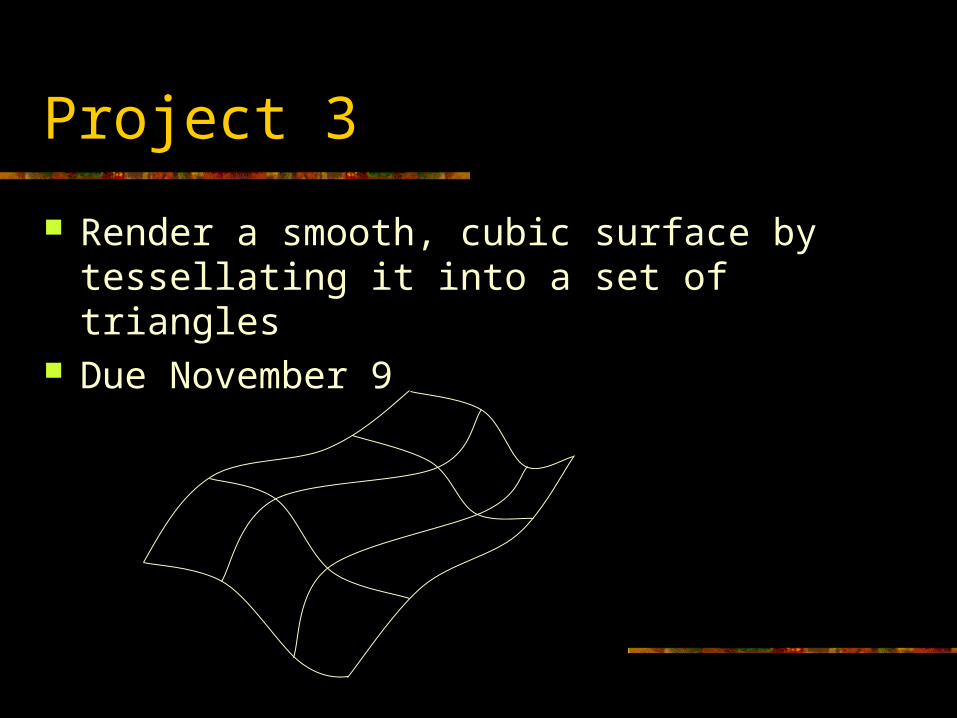
Project 3

Render a smooth, cubic surface by tessellating it into a set of triangles

Due November 9

Polynomial Functions

Linear:

Quadratic:

Cubic:

dctbtattf

cbtattf

battf

23

2

Vector Polynomials (Curves)

Linear:

Quadratic:

Cubic:

We usually define the curve for 0 ≤ t ≤ 1

dcbaf

cbaf

baf

tttt

ttt

tt

23

2

Linear Interpolation

Linear interpolation (Lerp) is a common technique for generating a new value that is somewhere in between two other values

A ‘value’ could be a number, vector, color, or even something more complex like an entire 3D object…

Consider interpolating between two points a and b by some parameter t

baba tttLerp 1,,

a

b

t=1.

. 0<t<1t=0

Bezier Curves

Bezier curves can be thought of as a higher order extension of linear interpolation

p0

p1

p0

p1p2

p0

p1

p2

p3

Linear Quadratic Cubic

Bezier Curve Formulation

There are lots of ways to formulate Bezier curves mathematically. Some of these include: de Castlejau (recursive linear interpolations) Bernstein polynomials (functions that define the

influence of each control point as a function of t) Cubic equations (general cubic equation of t) Matrix form

We will briefly examine each of these

Bezier Curve

p0

p1

p2

p3

Find the point x on the curve as a function of parameter t:

x(t)•

de Casteljau Algorithm

The de Casteljau algorithm describes the curve as a recursive series of linear interpolations

This form is useful for providing an intuitive understanding of the geometry involved, but it is not the most efficient form

de Casteljau Algorithm

p0

p1

p2

p3

We start with our original set of points

In the case of a cubic Bezier curve, we start with four points

de Casteljau Algorithm

p0

q0

p1

p2

p3

q2

q1

322

211

100

,,

,,

,,

ppq

ppq

ppq

tLerp

tLerp

tLerp

de Casteljau Algorithm

q0

q2

q1

r1

r0

211

100

,,

,,

qqr

qqr

tLerp

tLerp

de Casteljau Algorithm

r1x

r0•

10 ,, rrx tLerp

Bezier Curve

x•

p0

p1

p2

p3

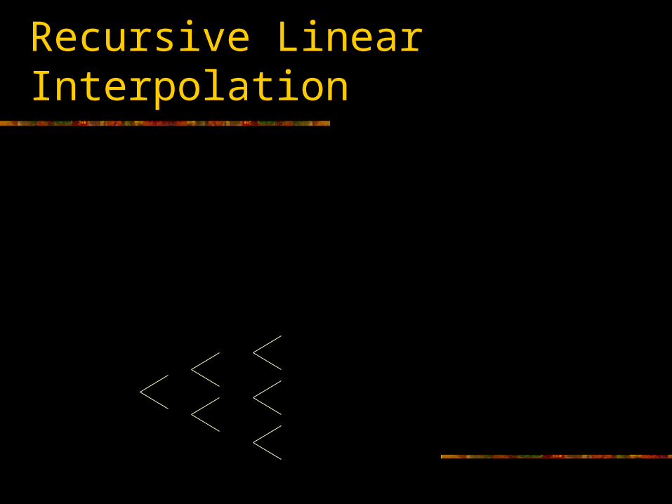
Recursive Linear Interpolation

322

211

100

,,

,,

,,

ppq

ppq

ppq

tLerp

tLerp

tLerp

211

100

,,

,,

qqr

qqr

tLerp

tLerp

10 ,, rrx tLerp

3

2

1

0

p

p

p

p

2

1

0

q

q

q

1

0

r

rx

3

2

1

0

p

p

p

p

Expanding the Lerps

3221

211010

3221211

2110100

32322

21211

10100

111

1111,,

111,,

111,,

1,,

1,,

1,,

pppp

pppprrx

ppppqqr

ppppqqr

ppppq

ppppq

ppppq

ttttttt

ttttttttLerp

tttttttLerp

tttttttLerp

tttLerp

tttLerp

tttLerp

Bernstein Polynomial Form

3

32

23

123

023

33

22

12

03

3221

2110

33

363133

13131

111

1111

pp

ppx

ppppx

pppp

ppppx

ttt

tttttt

tttttt

ttttttt

ttttttt

Cubic Bernstein Polynomials

33

3

2332

2331

2330

3332

321

310

30

33

223

123

023

33

363

133

33

363133

ttB

tttB

ttttB

ttttB

tBtBtBtB

ttt

tttttt

ppppx

pp

ppx

Bernstein Polynomials

B33B0

3

B13 B2

3

Bernstein Polynomials

1

!!

!1

122

12

33

363

133

11

10

222

221

220

333

2332

2331

2330

tB

ini

n

i

ntt

i

ntB

ttB

ttB

ttB

tttB

tttB

ttB

tttB

ttttB

ttttB

ni

iinni

Bernstein Polynomials

n

ii

ni

iinni

tBt

tti

ntB

0

1

px

Bernstein polynomial form of a Bezier curve:

Bernstein Polynomials

We start with the de Casteljau algorithm, expand out the math, and group it into polynomial functions of t multiplied by points in the control mesh

The generalization of this gives us the Bernstein form of the Bezier curve

This gives us further understanding of what is happening in the curve: We can see the influence of each point in the control

mesh as a function of t We see that the basis functions add up to 1, indicating

that the Bezier curve is a convex average of the control points

Cubic Equation Form

133

36333

33

363133

010

2210

33210

33

223

123

023

ppp

pppppppx

pp

ppx

t

tt

ttt

tttttt

Cubic Equation Form

0

10

210

3210

23

010

2210

33210

33

363

33

133

36333

pd

ppc

pppb

ppppa

dcbax

ppp

pppppppx

ttt

t

tt

Cubic Equation Form

If we regroup the equation by terms of exponents of t, we get it in the standard cubic form

This form is very good for fast evaluation, as all of the constant terms (a,b,c,d) can be precomputed

The cubic equation form obscures the input geometry, but there is a one-to-one mapping between the two and so the geometry can always be extracted out of the cubic coefficients

Cubic Matrix Form

0

10

210

3210

23

33

363

33

pd

ppc

pppb

ppppa

dcbax

ttt

3

2

1

0

23

0001

0033

0363

1331

1

p

p

p

p

d

c

b

a

d

c

b

a

x ttt

Cubic Matrix Form

zyx

zyx

zyx

zyx

ppp

ppp

ppp

ppp

ttt

ttt

333

222

111

000

23

3

2

1

0

23

0001

0033

0363

1331

1

0001

0033

0363

1331

1

x

p

p

p

p

x

Matrix Form

Ctx

GBtx

x

BezBez

zyx

zyx

zyx

zyx

ppp

ppp

ppp

ppp

ttt

333

222

111

000

23

0001

0033

0363

1331

1

Matrix Form

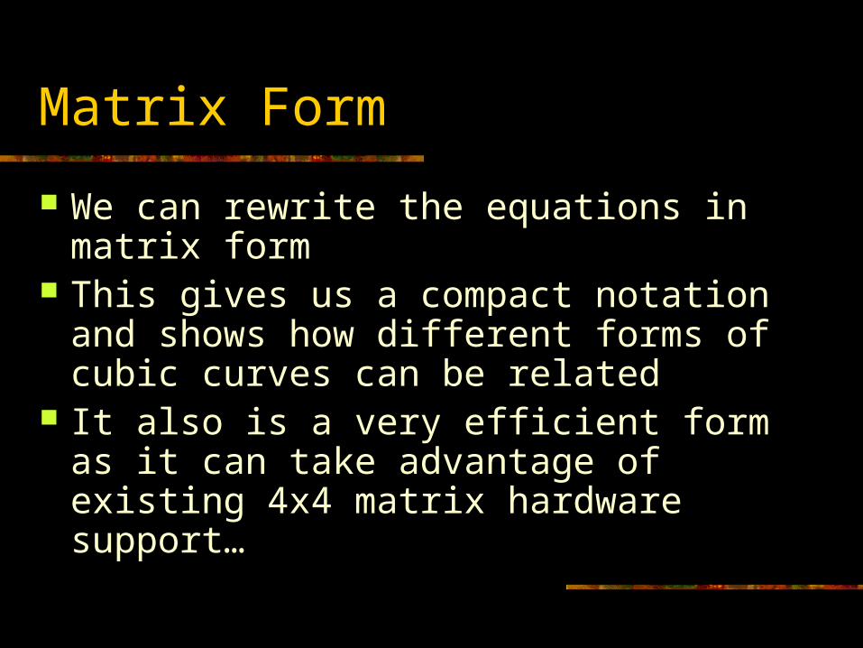
We can rewrite the equations in matrix form

This gives us a compact notation and shows how different forms of cubic curves can be related

It also is a very efficient form as it can take advantage of existing 4x4 matrix hardware support…

Bezier Curves & Cubic Curves

By adjusting the 4 control points of a cubic Bezier curve, we can represent any cubic curve

Likewise, any cubic curve can be represented uniquely by a cubic Bezier curve

There is a one-to-one mapping between the 4 Bezier control points (p0,p1,p2,p3) and the pure cubic coefficients (a,b,c,d)

The Bezier basis matrix BBez (and it’s inverse) perform this mapping

There are other common forms of cubic curves that also retain this property (Hermite, Catmull-Rom, B-Spline)

Derivatives

Finding the derivative (tangent) of a curve is easy:

cbax

dcbax ttdt

dttt 23 223

d

c

b

a

x

d

c

b

a

x 01231 223 ttdt

dttt

Tangents

The derivative of a curve represents the tangent vector to the curve at some point

tdt

dx

tx

Convex Hull Property

If we take all of the control points for a Bezier curve and construct a convex polygon around them, we have the convex hull of the curve

An important property of Bezier curves is that every point on the curve itself will be somewhere within the convex hull of the control points

p0

p1

p2

p3

Continuity

A cubic curve defined for t ranging from 0 to 1 will form a single continuous curve and not have any gaps

We say that it has geometric continuity, or C0 continuity We can easily see that the first derivative will be a

continuous quadratic function and the second derivative will be a continuous linear function

The third derivative (and all others) are continuous as well, but in a trivial way (constant), so we generally just say that a cubic curve has second derivative continuity or C2 continuity

In general, the higher the continuity value, the ‘smoother’ the curve will be, although it’s actually a little more complicated than that…

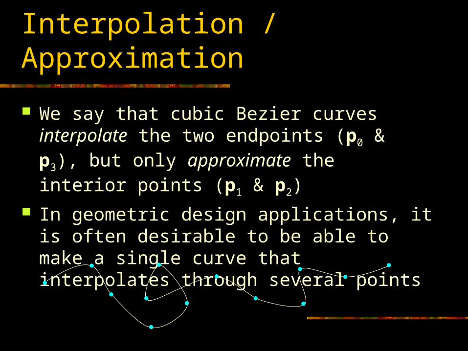
Interpolation / Approximation

We say that cubic Bezier curves interpolate the two endpoints (p0 & p3), but only approximate the interior points (p1 & p2)

In geometric design applications, it is often desirable to be able to make a single curve that interpolates through several points

Piecewise Curves

Rather than use a very high degree curve to interpolate a large number of points, it is more common to break the curve up into several simple curves

For example, a large complex curve could be broken into cubic curves, and would therefore be a piecewise cubic curve

For the entire curve to look smooth and continuous, it is necessary to maintain C1 continuity across segments, meaning that the position and tangents must match at the endpoints

For smoother looking curves, it is best to maintain the C2 continuity as well

Connecting Bezier Curves

A simple way to make larger curves is to connect up Bezier curves Consider two Bezier curves defined by p0…p3 and v0…v3

If p3=v0, then they will have C0 continuity If (p3-p2)=(v1-v0), then they will have C1 continuity C2 continuity is more difficult…

p0

p0

p1

p2

P3

P3

p2

p1

v0

v1

v2

v3

v3

v2

v1

v0

C0 continuity C1 continuity