1. Mean Boundary Layer CharacteristicsThe study of the boundary layer is on the small scale of meteorological motions.When we study turbulence, or scales roughly smaller than 3km, we are within themicroscale, hence Micrometeorology and Boundary Layer meteorology are virtu-ally synonyms.

1a. Why do we study the boundary layer?

• We live in the boundary layer.

• Main sources of pollution are within the BL

• Forecasts of dew, frost, Tmin and Tmax - which are so important for agri-culture.

• Evaporation from the oceans is very important as latent heat drives 80% ofatmospheric motions.

• Wind turbines and buildings are driven and affected by turbulence.

• I use boundary layer theory in my work because I am interested in evapo-transpiration - where it origiantes and where it later falls as precipitation.Transpiration from plants and evaporation moves through turbulent trans-port within the BL and is either advected horizontally or into the free atmo-sphere.

The boundary layer is different from the rest of the atmosphere because of theinfluence of the earth on the air. The surface modifies the lowest 100 to 3000mTHIS is the boundary layer. The emphasis of this class will be in the midlatitudeboundary layer because of the abundant measurements.

1b. Definition of the Boundary Layer

”Part of the troposphere that is directly influenced by the presence of the earth’ssurface, and responds to the surface forcings with a timescale of about an hour orless”. Even though the entire troposphere responds, the response outside the BLis slow. For example, the diurnal variation of temperature near the ground is muchmore evident than at high altitudes. TURBULENCE is one of the most important

1

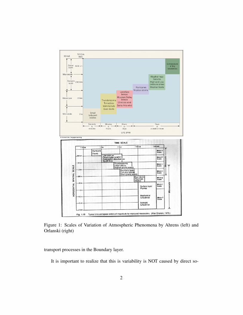
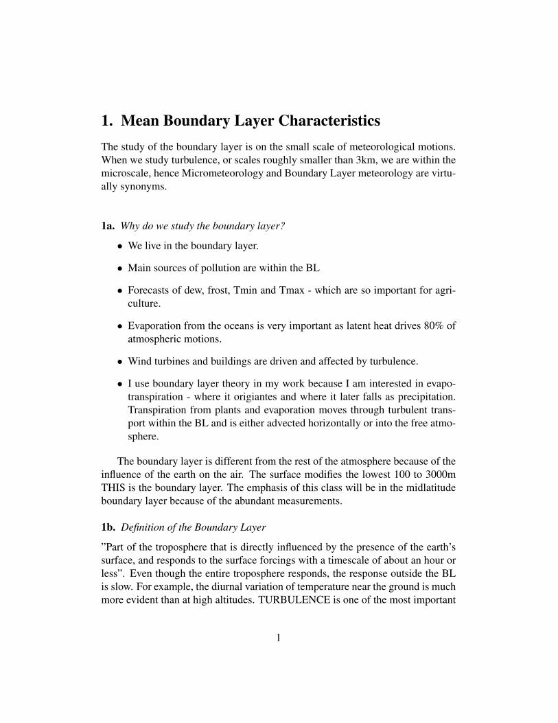
Figure 1: Scales of Variation of Atmospheric Phenomena by Ahrens (left) andOrlanski (right)

transport processes in the Boundary layer.

It is important to realize that this is variability is NOT caused by direct so-

2

Figure 2: Temperature Variations for a location in the Central United States. May1988

lar forcing. The earth emits longwave radiation and heats the atmospehre. Theground absorbs close to 90% of incoming radiation, so it is nearly a black body.

Question: What are the forcings that the earth exerts on the atmosphere?Answer: Frictional Drag, Evaporation, Transpiration, Heat transfer, Pollutantemission, Terrain induced flow modification.

1c. How do we study the Boundary Layer?

You cannot deterministically describe each eddy, because they are very small andvary rapidly in time. To study turbulence scientist use three avenues:

3

1. Stochastic methods: average statistical effects fo the eddies.

2. Similarity theory: common behavior of observed phenomena when scaled.

3. Phenomenological classifications: large eddies such as thermals are par-tially deterministically described.

Field experiments, numerical and laboratory simulations have all been used tounderstand turbulence.

1d. Clouds in the Boundary Layer

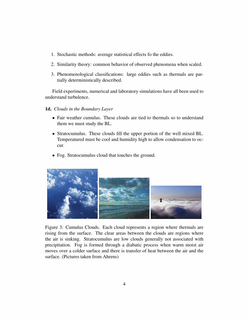
• Fair weather cumulus. These clouds are tied to thermals so to understandthem we must study the BL.

• Stratocumulus. These clouds fill the upper portion of the well mixed BL.Temperatured must be cool and humidity high to allow condensation to oc-cur.

• Fog. Stratocumulus cloud that touches the ground.

Figure 3: Cumulus Clouds. Each cloud represents a region where thermals arerising from the surface. The clear areas between the clouds are regions wherethe air is sinking. Stratocumulus are low clouds generally not associated withprecipitation. Fog is formed through a diabatic process when warm moist airmoves over a colder surface and there is transfer of heat between the air and thesurface. (Pictures taken from Ahrens)

4

1e. Wind and Flow

Within the boundary layer we can have mean wind, turbulence and waves.

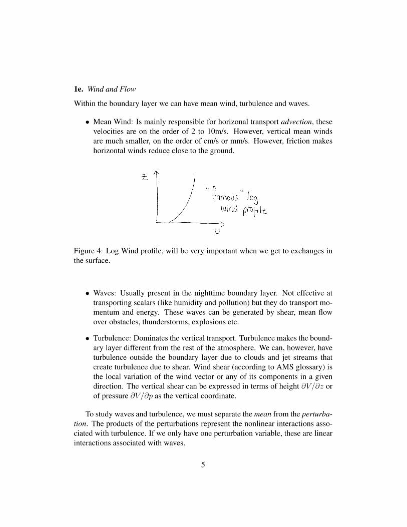
• Mean Wind: Is mainly responsible for horizonal transport advection, thesevelocities are on the order of 2 to 10m/s. However, vertical mean windsare much smaller, on the order of cm/s or mm/s. However, friction makeshorizontal winds reduce close to the ground.

Figure 4: Log Wind profile, will be very important when we get to exchanges inthe surface.

• Waves: Usually present in the nighttime boundary layer. Not effective attransporting scalars (like humidity and pollution) but they do transport mo-mentum and energy. These waves can be generated by shear, mean flowover obstacles, thunderstorms, explosions etc.

• Turbulence: Dominates the vertical transport. Turbulence makes the bound-ary layer different from the rest of the atmosphere. We can, however, haveturbulence outside the boundary layer due to clouds and jet streams thatcreate turbulence due to shear. Wind shear (according to AMS glossary) isthe local variation of the wind vector or any of its components in a givendirection. The vertical shear can be expressed in terms of height ∂V/∂z orof pressure ∂V/∂p as the vertical coordinate.

To study waves and turbulence, we must separate the mean from the perturba-tion. The products of the perturbations represent the nonlinear interactions asso-ciated with turbulence. If we only have one perturbation variable, these are linearinteractions associated with waves.

5

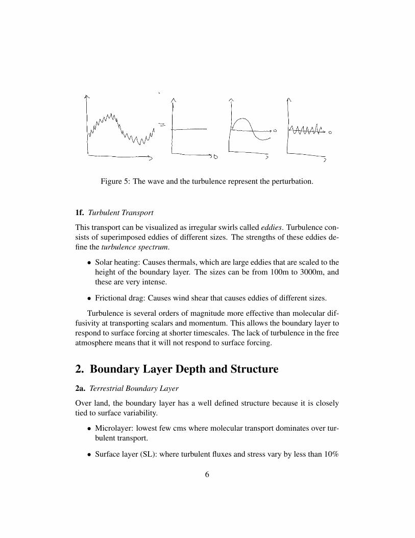
Figure 5: The wave and the turbulence represent the perturbation.

1f. Turbulent Transport

This transport can be visualized as irregular swirls called eddies. Turbulence con-sists of superimposed eddies of different sizes. The strengths of these eddies de-fine the turbulence spectrum.

• Solar heating: Causes thermals, which are large eddies that are scaled to theheight of the boundary layer. The sizes can be from 100m to 3000m, andthese are very intense.

• Frictional drag: Causes wind shear that causes eddies of different sizes.

Turbulence is several orders of magnitude more effective than molecular dif-fusivity at transporting scalars and momentum. This allows the boundary layer torespond to surface forcing at shorter timescales. The lack of turbulence in the freeatmosphere means that it will not respond to surface forcing.

2. Boundary Layer Depth and Structure2a. Terrestrial Boundary Layer

Over land, the boundary layer has a well defined structure because it is closelytied to surface variability.

• Microlayer: lowest few cms where molecular transport dominates over tur-bulent transport.

• Surface layer (SL): where turbulent fluxes and stress vary by less than 10%

6

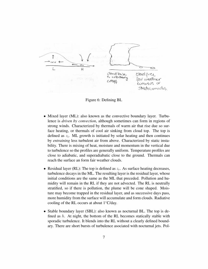
Figure 6: Defining BL

• Mixed layer (ML): also known as the convective boundary layer. Turbu-lence is driven by convection, although sometimes can form in regions ofstrong winds. Characterized by thermals of warm air that rise due so sur-face heating, or thermals of cool air sinking from cloud top. The top isdefined as zi. ML growth is initiated by solar heating and then continuesby entraining less turbulent air from above. Characterized by static insta-bility. There is mixing of heat, moisture and momentum in the vertical dueto turbulence so the profiles are generally uniform. Temperature profiles areclose to adiabatic, and superadiabatic close to the ground. Thermals canreach the surface an form fair weather clouds.

• Residual layer (RL): The top is defined as zr. As surface heating decreases,turbulence decays in the ML. The resulting layer is the residual layer, whoseinitial conditions are the same as the ML that preceded. Pollution and hu-midity will remain in the RL if they are not advected. The RL is neutrallystratified, so if there is pollution, the plume will be cone shaped. Mois-ture may become trapped in the residual layer, and as successive days pass,more humidity from the surface will accumulate and form clouds. Radiativecooling of the RL occurs at about 1◦C/day.

• Stable boundary layer (SBL): also known as nocturnal BL. The top is de-fined as h. At night, the bottom of the RL becomes statically stable withsporadic turbulence. It blends into the RL without a clearly defined bound-ary. There are short bursts of turbulence asociated with nocturnal jets. Pol-

7

Figure 7: Mixed Layer Profiles

lutants disperse little in the vertical, they ”fan out” in the horizontal. Youcan also have a SBL during the day if the surface is colder than the overlyingair. Waves are common in the SBL.

• Cloud layer (CL) and subcloud layer (SCL): when clouds are present. Thetop is defined as zb close to the LCL.

2b. Virtual Potential Temperature Evolution.

Notice that while both the ML and RL are adiabatic, the ML is statically unstableand the RL is statically neutral. To know the static stability we must look at thelayer immediately below and immediately above.

2c. Static Stability

Static stability is a measure of the capability for buoyant convection. It doesn’tdepend on wind. When less dense air underlies denser air, there is static instabilityand the atmosphere will begin to allow convection and thermals will form.

8

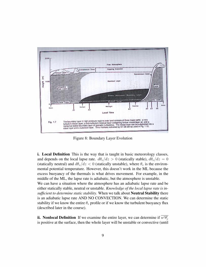
Figure 8: Boundary Layer Evolution

i. Local Definition This is the way that is taught in basic meteorology classes,and depends on the local lapse rate. dθv/dz > 0 (statically stable), dθv/dz = 0(statically neutral) and dθv/dz < 0 (statically unstable), where θv is the environ-mental potential temperature. However, this doesn’t work in the ML because theexcess buoyancy of the thermals is what drives movement. For example, in themiddle of the ML, the lapse rate is adiabatic, but the atmosphere is unstable.We can have a situation where the atmosphere has an adiabatic lapse rate and beeither statically stable, neutral or unstable. Knowledge of the local lapse rate is in-sufficient to determine static stability. When we talk about Neutral Stability thereis an adiabatic lapse rate AND NO CONVECTION. We can determine the staticstability if we know the entire θv profile or if we know the turbulent buoyancy flux(described later in the course).

ii. Nonlocal Definition If we examine the entire layer, we can determine if w′θ′vis positive at the surface, then the whole layer will be unstable or convective (until

9

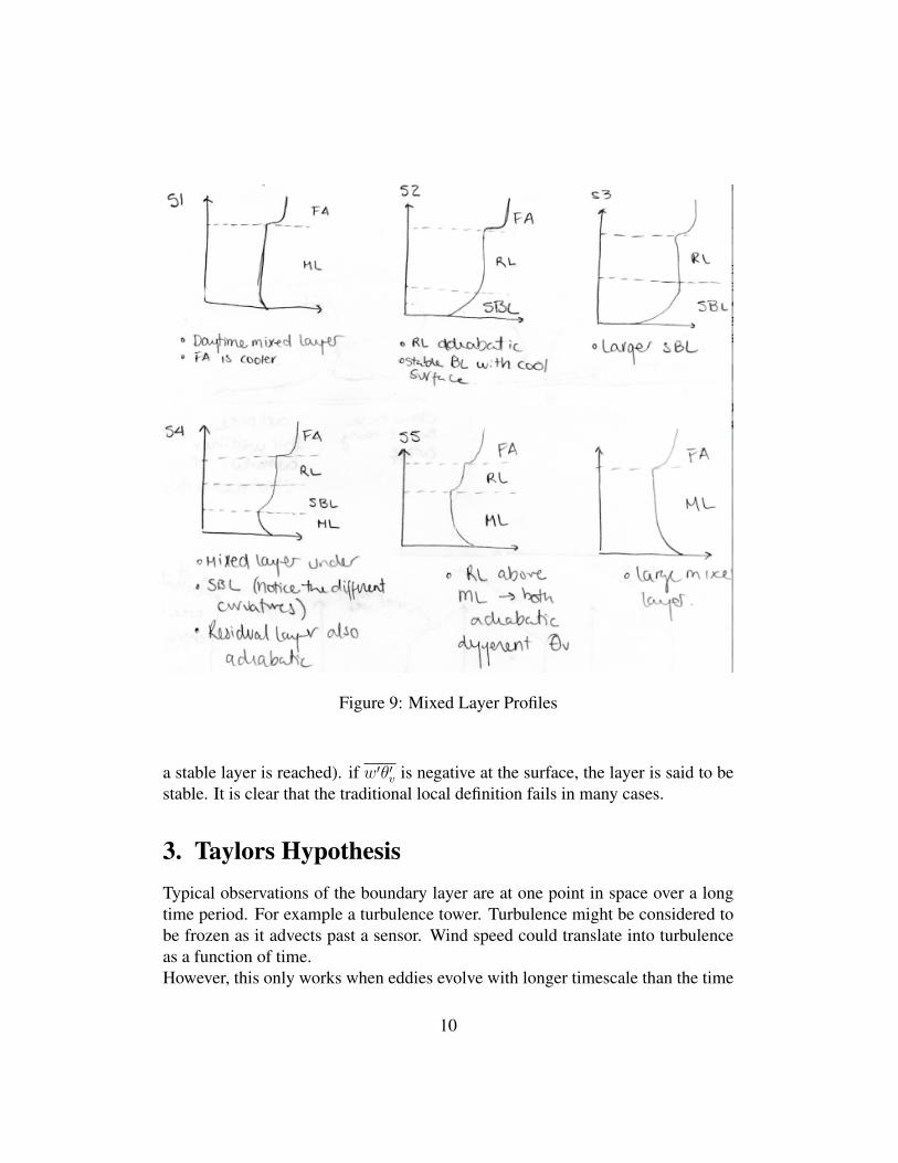
Figure 9: Mixed Layer Profiles

a stable layer is reached). if w′θ′v is negative at the surface, the layer is said to bestable. It is clear that the traditional local definition fails in many cases.

3. Taylors HypothesisTypical observations of the boundary layer are at one point in space over a longtime period. For example a turbulence tower. Turbulence might be considered tobe frozen as it advects past a sensor. Wind speed could translate into turbulenceas a function of time.However, this only works when eddies evolve with longer timescale than the time

10

it takes the eddy to be advected past the sensor.

Let U and V represent the zonal (eastward) and meridional (northward) windcomponents. M represents the total wind magnitudeM2 = U2+V 2. If an eddy ofdiameter λ is advected by the mean wind, then the time P for it to pass a stationarysensor is:

P =λ

M(1)

λ = MP (2)

Also, if we use the wavenumber k = 2π/λ, and the frequency f = 2π/P ,then Equation 2 becomes:

f = Mk (3)

iii. Exercise Figure 12 shows wind measured in the early afternoon.

• What is the mean wind between noon and 12:30? What is the mean windbetween 2pm and 2:30pm?

• Is the intensity of turbulence constant or does it vary? How can you tell?

• Looking closely at the graph, there are peaks that ocur every minute, whileothers have periodicity of about 10 minutes. What are the range of sizes ofeddies in the first and the second half of the period?

11

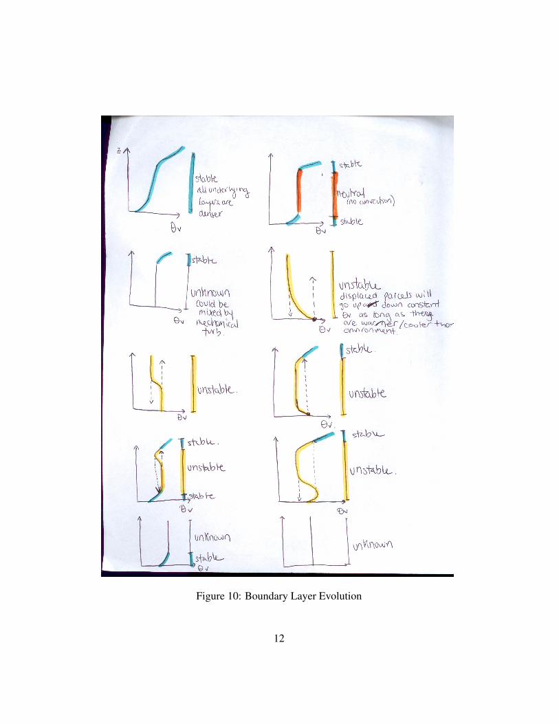
Figure 10: Boundary Layer Evolution

12

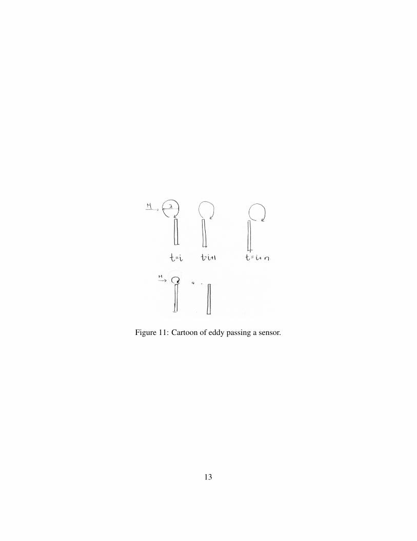
Figure 11: Cartoon of eddy passing a sensor.

13

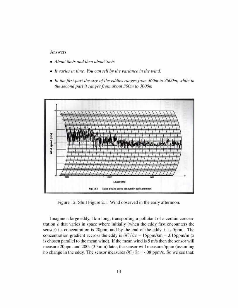
Answers

• About 6m/s and then about 5m/s

• It varies in time. You can tell by the variance in the wind.

• In the first part the size of the eddies ranges from 360m to 3600m, while inthe second part it ranges from about 300m to 3000m

Figure 12: Stull Figure 2.1. Wind observed in the early afternoon.

Imagine a large eddy, 1km long, transporting a pollutant of a certain concen-tration ρ that varies in space where initially (when the eddy first encounters thesensor) its concentration is 20ppm and by the end of the eddy, it is 5ppm. Theconcentration gradient accross the eddy is ∂C/∂x = 15ppm/km = .015ppm/m (xis chosen parallel to the mean wind). If the mean wind is 5 m/s then the sensor willmeasure 20ppm and 200s (3.3min) later, the sensor will measure 5ppm (assumingno change in the eddy. The sensor measures ∂C/∂t = -.08 ppm/s. So we see that:

14

Figure 13: Example Taylor’s Hypothesis

∂C

∂t= −M∂C

∂x(4)

Equation 4 represents Taylor’s Hypothesis for concentration in onedimension.

In this particular case, ∂C∂t

= -5m/s * .015 ppm/m = .08 ppm/s.In the more general case, Taylor’s Hypothesis states that turbulence is frozen

when the total derivative dξ/dt = 0. Where ξ is any variable that can vary in timeand any direction. REMEMBER, the total derivative is defined by:

dξ

dt=∂ξ

∂t+∂ξ

∂x

∂x

∂t+∂ξ

∂y

∂y

∂t+∂ξ

∂z

∂z

∂t(5)

dξ

dt=∂ξ

∂t+∂ξ

∂xU +

∂ξ

∂yV +

∂ξ

∂zW (6)

since the total derivative is zero for Taylor’s Hypothesis,

∂ξ

∂t= −U ∂ξ

∂x− V

∂ξ

∂y−W

∂ξ

∂z(7)

15