Erik SwansonCori Saviano

Li ZhaFinal Project

1 Introduction

In analyzing time series data, we are posed with the question of how past events influencesthe current situation. In order to determine this, we usually impose a model on our datathat involves a number of lag terms. The coefficients on these lag terms give us informationabout the effects of past events, and should help us predict future values for whateverdependent variable we are studying. However, in adding additional lag terms, we are gaininginformation, but at the same time sacrificing simplicity.

When the true model is not known (which it rarely is) we run the risk of over-specifyingor under-specifying the model by adding too many or too few lags. The Bayesian informationcriterion and the Akaike information criterion can help in regularization of our model. Thesecriterion attempt to balance the information gained by adding additional lags against theincrease in the complexity of the model that these lags cause.

In order to determine how effective these methods of regularization are, we must know thetrue specification of the model. Since this would be a difficult, if not impossible, task with realeconomic data, the problem lends itself well to Monte Carlo simulation. In this simulationwe will be randomly generating data to create a wide variety of time-series specifications,and then analyzing the efficacy of the AIC and SBIC in predicting the true model underthese varying circumstances.

2 AIC versus SBIC

When we make choices about the order p of an autoregression, we have to balance themarginal benefit of including more lags against the marginal cost of increased uncertaintyof estimation. If we do not include enough lags, we run the risk of omitting potentiallysignificant information contained in more distant lags. On the other hand, with too manylags we estimate more coefficients than needed. This practice might in turn lead to estimationerrors.

One approach to choosing the appropriate p is to perform hypothesis tests on the finallag. For example, we start from estimating an AR(4) model and test whether the coefficienton the fourth lag is significant at the appropriate significance levels, say 5%. If it is notsignificant, we drop it and estimate AR(3) model, and so on. One drawback of this t-statistics approach is that such tests would incorrectly reject the null hypothesis of zerocoefficient 5% of the time. To put in another way, when the true number of lags is four, thet-statisitic approach would estimate p to be six 5% of the time.

1

An alternative approach to get around this problem is to estimate p by using “informa-tion criterion,” such as Akaike information criterion (AIC) and Bayes informationcriterion (BIC), also known as Schwartz information criterion (SIC). These informa-tion criteria are designed explicitly for model selection. Model selection criteria generallyinvolve information criteria function calculations for each of the models. We pick the modelfor which the function is maximized or minimized. Stata calculates the AIC and BIC resultsbased on their standard definitions, which include the constant term from the log likelihoodfunction. Stata uses the following form of log likelihood function (LL) for VAR(p), as shownby Hamilton (1994, 295-296).

LL = (T

2){ln(|Σ̂−1|)−K ln(2π)−K}

where T is the number of observations, K is the number of equations, and Σ̂ is themaximum likelihood estimate of E[utu

′t], where ut is the K × 1 vector of disturbances.

Because

ln(|Σ̂−1|) = −ln(|Σ̂|)

we can rewrite the log likelihood as

LL = −(T

2){ln(|Σ̂|) +K ln(2π) +K}

.

Stata uses the following definitions of AIC and BIC function based on the log likelihoodfunction defined above.

AIC(p) = −2(LL

T) + 2

tpT

BIC(p) = −2(LL

T) +

ln (T )

Ttp

where LL stands for the log likelihood for a VAR(p) (shown above), T is the number ofobservations, and p is the number of lags.

Note that STATA’s suggestion for the ideal lag length is the minimization of the AICand BIC functions.

In most cases, we prefer the model that has fewest parameter to estimate, provided thateach one of the candidate models is correctly specified. This is called the most parsimoniousmodel of the set. The AIC does not always suggests the most parsimonious model, becausethe AIC function is largely based on the log likelihood function. Davidson and McKinnon(2004, 676) indicates that whenever two or more models are nested, the AIC may fail tochoose the most parsimonious one, if that these models are correctly specified. In anothercase, if all the models are nonnested, and only one is well specified, the AIC chooses the well-specified model asymptotically, because this model has the largest value of the log likelihoodfunction.

2

The Bayesian information criterion (BIC) avoids the problem discussed above by replac-ing 2 in the AIC function with the ln(T ) term. As T →∞, the addition of another lag wouldincrease the BIC value by a larger margin. Hence, asymptotically, BIC would pick the moreparsimonious model than AIC might suggest.

Stock and Watson (2007) recommends that we choose the model suggested by AIC ratherthan BIC. They argue that including more parameters is better than omitting significantparameters.

In this project, we seek to examine how well the AIC and BIC predict the lag lengthscorrectly in two cases. First, the lag coefficients are abruptly truncated. Second, the lagcoefficients decline linearly. We used simulation experiments, often referred to as MonteCarlo experiments extensively in our tests. Monte Carlo experiments is the topic in thenext section.

3 Monte Carlo Studies

Monte Carlo studies is the simulation of the behavior of the estimators under controlledconditions that may deviate from the standard assumptions. Monte Carlo experiments allowus to vary some parameters that in actual cases are fixed and test how changes in theseparameters affect the test statistics, for example, the AIC or BIC results.

The first step in Monte Carlo studies is to generate data for simulations, We can use actualvariables from real data sets or generate data from random-number generator (RNG).Note that because most RNGs require a specification of the first term of the sequence, theseed, the data generating process is not purely random. RNGs generate later terms in thesequence based on calculations. Many RNGs generate numbers that appear to be drawingsfrom the uniform U(0, 1) distribution. Another popular choice is to draw from the normaldistribution with mean and standard deviation given, such as N(0, 1).

When we implement the Monte Carlo experiment, we specify the number of repeatedsamples and the test statistics of interest (AIC and BIC) to be calculated in each simulation.We must also take great care to accumulate the estimates of the test statistics in a new dataset.

Once we obtained the simulation results, we need to examine the properties of the es-timates. For example, we calculate the mean and standard deviation, or use quantiles toassess critical values (for example, the predetermined lag length in our study.)

4 Data Generation Process

As stated above, the first step of a Monte Carlo simulation is the data generation process.In generating our data, we must consider what selection of the possible models we want toanalyze. We choose to analyze the following changes.

• Abrubtly declining versus gradually declining lag coefficients

3

• The number of lags

• Autocorrelation of the X values

• Number of observations

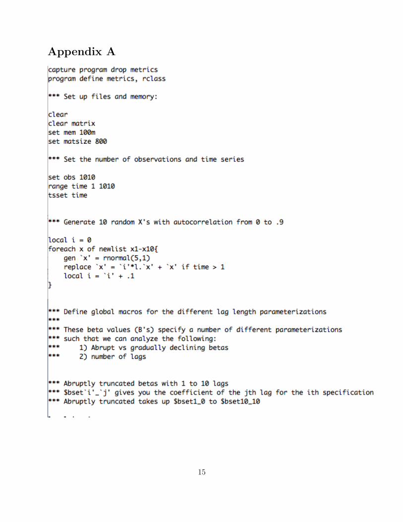
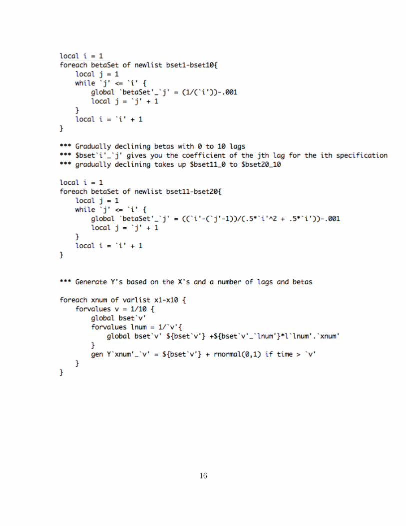
Here we will describe our method for generating the data. The data is generated throughthe use of a Stata .do file, which can be found in Appendix A. The end result of our datagenerating process is a number of models which share the form:

Yt = β00 + β0Xt + β1Xt−1 + β2Xt−2 + . . .+ βpXt−p + ut

This is an time series regression, but it is not auto regressive. The X values in this modelwill be generated independently of the Y values. As can be seen in the equation above,our Y values are dependent on the distribution of the error term, the distribution of the Xvalues, and the number and magnitude of the lag coefficients.

The first step in the data generating process is to generate a number of Xt values thatwe will later apply our lag coefficients to. Since one of the changes we want to analyze is theautocorrelation of X values, they are a first order autoregressive with the following form:

Xt = αZt−1 + Zt

Where Zt is a normally distributed random variable with mean 5 and standard deviation5. In our models we specify 10 different values for α, ranging from 0 to 0.9. We will eventuallypair each of these sets of X values with each of our specifications for the lag coefficients.First however, we must create our specification for the variation in number and magnitudeof lag coefficients.

Our models are created with numbers of lags including each of 1 to 10 lag coefficients.for both abruptly truncated and gradually declining coefficients. The method behind ourgeneration of these coefficients is that we want the effects of X to be as close to stationarityas possible. This will ensure that we are creating the most significant coefficients that wecan, with the effect that we are not giving unreasonably small coefficients for AIC and SBICto pick up.

To that end, if we are to have constant coefficients on the number of lags, the coefficientmust be less than one over the number of lags for the process to be stationary. In our process,we use the following formula to calculate the coefficients for our constant lag value, where pis the number of lags and β is the coefficient on all of these lags:

β =1

p− .001

If we are to have decreasing lags, an interesting specification for the lag coefficientswould be one in which the coefficients are linearly decreasing. The following equation givesus linearly decreasing coefficients for each n of p lags, and is stationary in its first difference.That is, it has a single unit root.

4

βn =p− (n− 1)

12p2 + 1

2p

However, we can achieve stationarity without differences if we subtract a small amountfrom each coefficient. So, in our data generation process we use the following equation togenerate our lag coefficients:

βn =p− (n− 1)

12p2 + 1

2p− .001

Then, with these lag coefficients, and our X values, we construct our models for Yt. Forsimplicity, we assume that the values of β00 and β0, as seen in the equation for Yt above, areequal to zero. This leaves us with

Yt = β1Xt−1 + β2Xt−2 + . . .+ βpXt−p + ut

.Where ut is a random normal distribution with mean zero and standard deviation one.

Since we have ten Xt series, ten lag specifications with abruptly truncated coefficients, andten lag specifications with gradually decreasing coefficients, a single run of our simulationgenerates 200 Yt series.

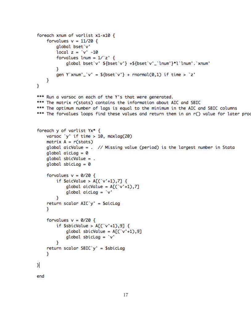
The next step in a Monte Carlo simulation is the definition of the test to be performed,and the number of times it is performed. For each of our 200 Yt series we have Stataperform an AIC and SBIC test, and store the number of predicted lags associated with eachparameterization of Yt. This gives us 400 final data points for a single run of the simulation.We then use Stata’s simulate command to run this simulation 100 times for both Yt witht = 100, and t = 1000. The following section will present our results and analysis of thechanges defined at the start of this section.

5 Data and Analysis

We begin our analysis with the simulation with 100 observations for each Yt. This is arelatively small sample size, but not unreasonably small for some time series analyses. Inthis smaller sample size, we might predict that, since AIC tends to be less parsimonious thanSBIC, that AIC would predict a larger number of lags on average.

5

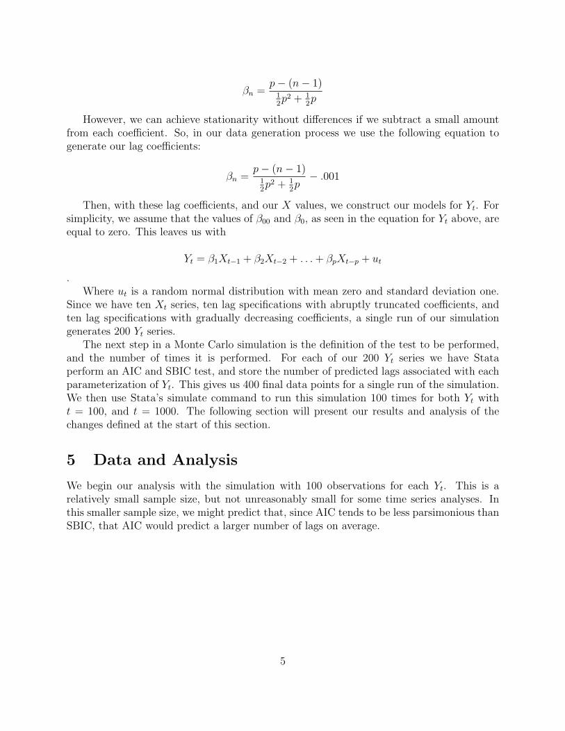
The graphs above plot the average predicted number of lags for the 100 runs of the

6

simulation (across all X’s) against the actual lags in the abruptly truncated model. Sincethese graphs are on the same scale, it is easy to see that the AIC predicts larger lag lengthsthan the SBIC. Still, both under-specify related to the true model after 6 and 2 lags for AICand SBIC respectively.

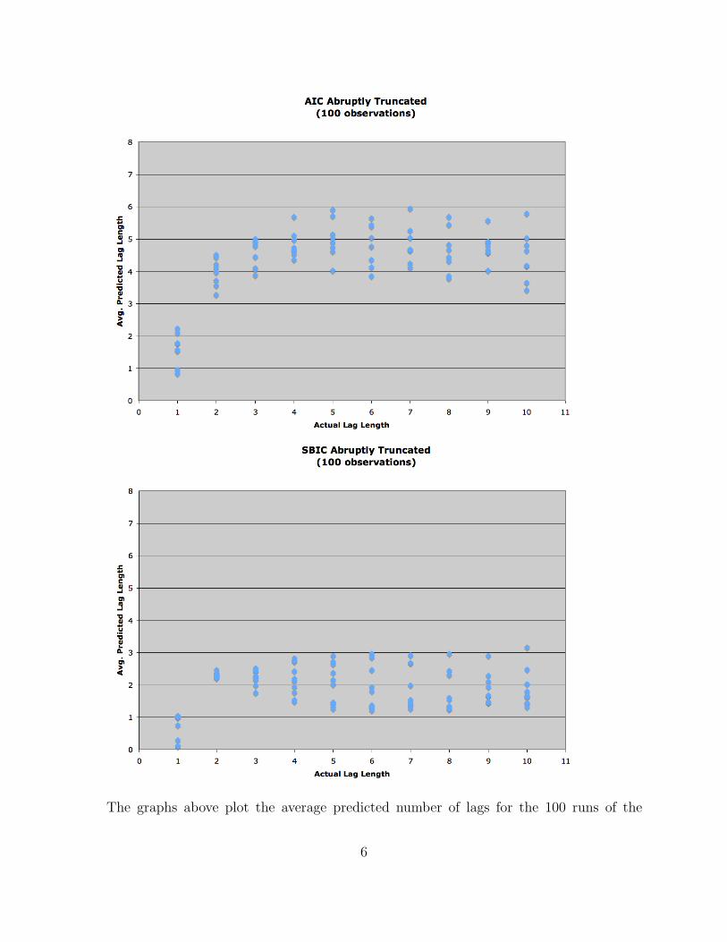
This under-specification is even more pronounced when we have gradually decreasing lagcoefficients. As can be seen in the graphs below, the AIC under-specifies the model after 4true lags.

7

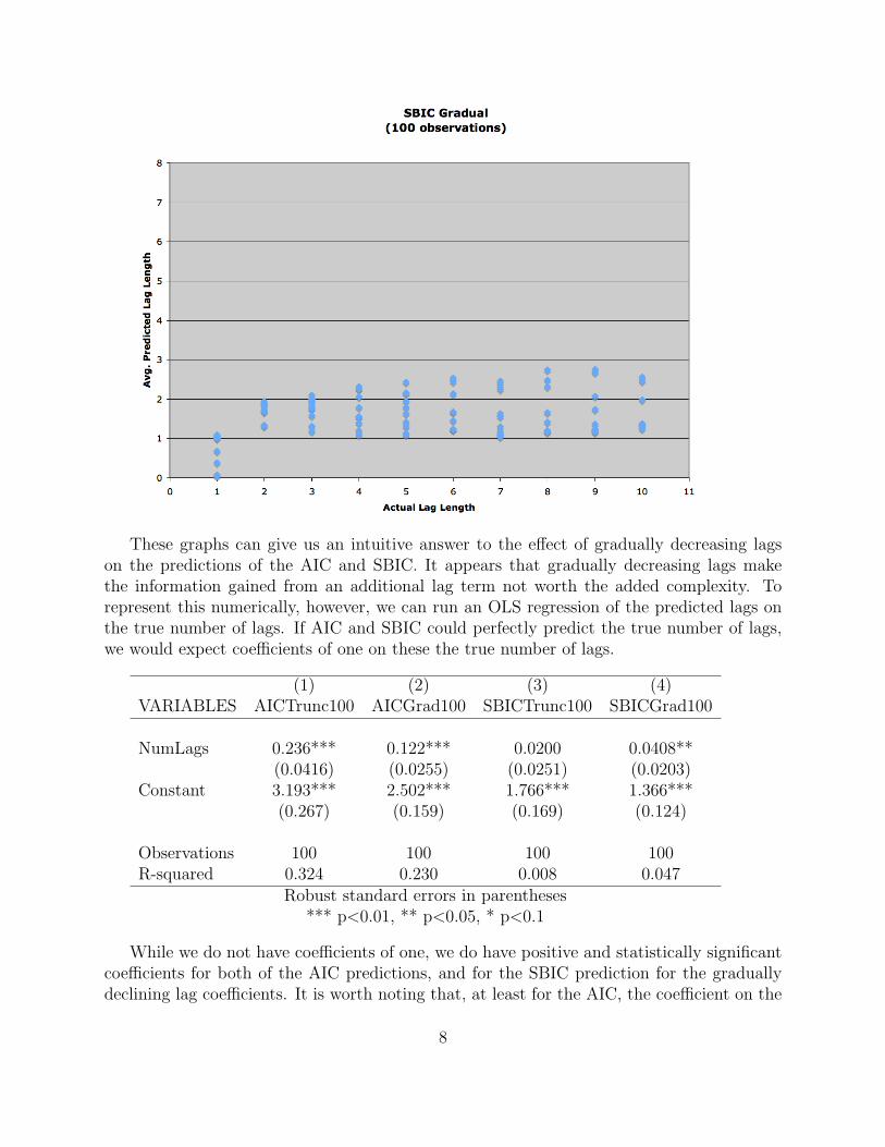
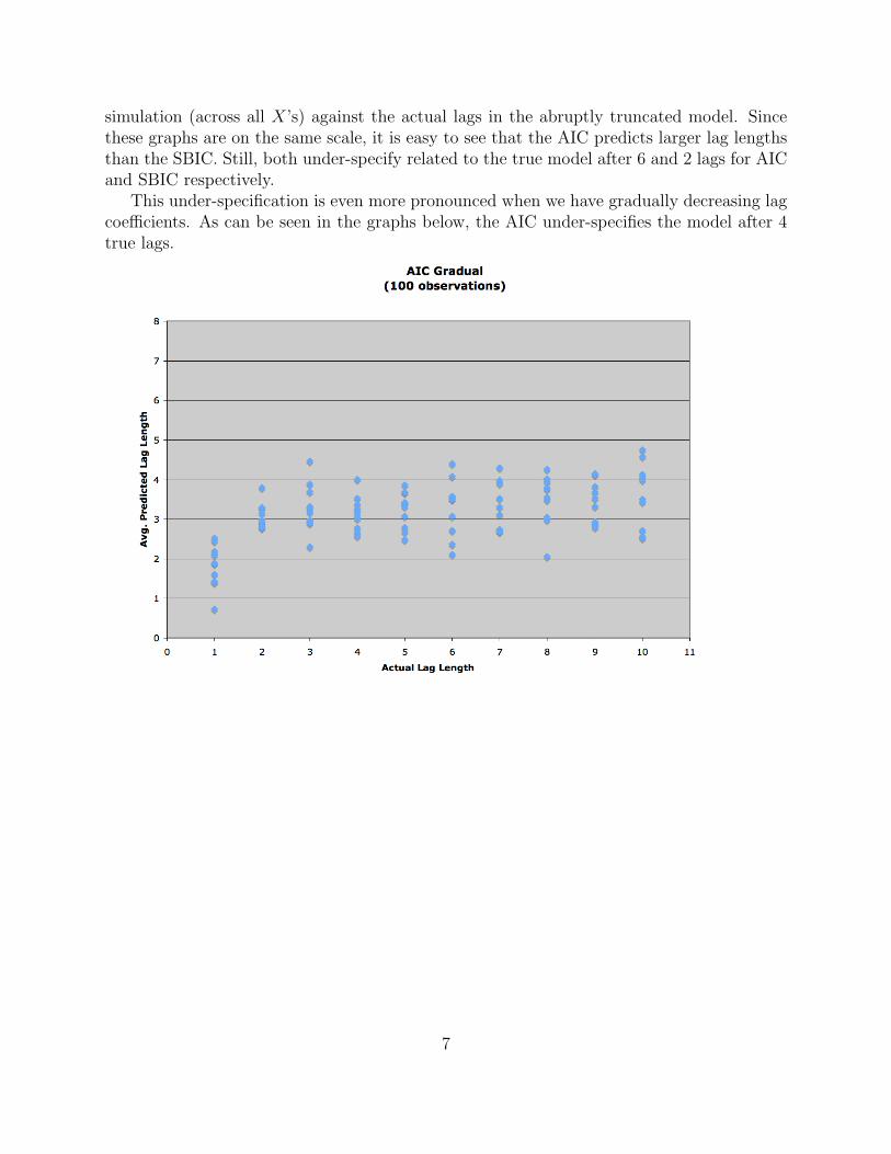
These graphs can give us an intuitive answer to the effect of gradually decreasing lagson the predictions of the AIC and SBIC. It appears that gradually decreasing lags makethe information gained from an additional lag term not worth the added complexity. Torepresent this numerically, however, we can run an OLS regression of the predicted lags onthe true number of lags. If AIC and SBIC could perfectly predict the true number of lags,we would expect coefficients of one on these the true number of lags.

(1) (2) (3) (4)VARIABLES AICTrunc100 AICGrad100 SBICTrunc100 SBICGrad100

NumLags 0.236*** 0.122*** 0.0200 0.0408**(0.0416) (0.0255) (0.0251) (0.0203)

Constant 3.193*** 2.502*** 1.766*** 1.366***(0.267) (0.159) (0.169) (0.124)

Observations 100 100 100 100R-squared 0.324 0.230 0.008 0.047

Robust standard errors in parentheses*** p<0.01, ** p<0.05, * p<0.1

While we do not have coefficients of one, we do have positive and statistically significantcoefficients for both of the AIC predictions, and for the SBIC prediction for the graduallydeclining lag coefficients. It is worth noting that, at least for the AIC, the coefficient on the

8

number of lags for the truncated lag coefficients is larger than for gradually declining lags.It is also worth noting that all of these coefficients would likely be closer to one if less lagswere included in the independent variable.

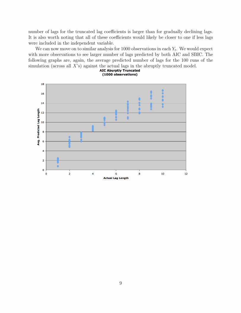
We can now move on to similar analysis for 1000 observations in each Yt. We would expectwith more observations to see larger number of lags predicted by both AIC and SBIC. Thefollowing graphs are, again, the average predicted number of lags for the 100 runs of thesimulation (across all X’s) against the actual lags in the abruptly truncated model.

9

As can be seen in the first graph, the AIC over-specifies the model for all values of thetrue lags, but has a fairly linear trend. The SBIC model, however, exhibits some strangebehavior, as it’s predicted number of lags seems to curve downward after five true lags. Thisis almost certainly a product of our specification for generating the lag coefficients as thenumber of lags increases. In our method for generating these coefficients, as more lags wereadded, the magnitude of all of the coefficients decreased fairly significantly. Before this,however, we see a fairly consistent, if slightly over-specified trend.

Next we can look at the predictions when we have 1000 observations and graduallydeclining lag coefficients.

10

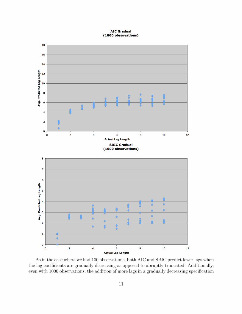
As in the case where we had 100 observations, both AIC and SBIC predict fewer lags whenthe lag coefficients are gradually decreasing as opposed to abruptly truncated. Additionally,even with 1000 observations, the addition of more lags in a gradually decreasing specification

11

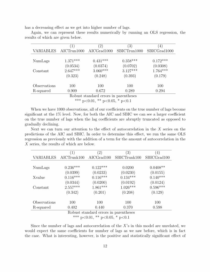
has a decreasing effect as we get into higher number of lags.Again, we can represent these results numerically by running an OLS regression, the

results of which are given below.

(1) (2) (3) (4)VARIABLES AICTrun1000 AICGrad1000 SBICTrun1000 SBICGrad1000

NumLags 1.371*** 0.431*** 0.358*** 0.172***(0.0534) (0.0374) (0.0702) (0.0308)

Constant 2.647*** 3.060*** 3.127*** 1.764***(0.323) (0.248) (0.393) (0.179)

Observations 100 100 100 100R-squared 0.909 0.672 0.289 0.294

Robust standard errors in parentheses*** p<0.01, ** p<0.05, * p<0.1

When we have 1000 observations, all of our coefficients on the true number of lags becomesignificant at the 1% level. Now, for both the AIC and SBIC we can see a larger coefficienton the true number of lags when the lag coefficients are abruptly truncated as opposed togradually declining.

Next we can turn our attention to the effect of autocorrelation in the X series on thepredictions of the AIC and SBIC. In order to determine this effect, we run the same OLSregression as previously with the addition of a term for the amount of autocorrelation in theX series, the results of which are below.

(1) (2) (3) (4)VARIABLES AICTrunk100 AICGrad100 SBICTrunk100 SBICGrad100

NumLags 0.236*** 0.122*** 0.0200 0.0408**(0.0399) (0.0233) (0.0230) (0.0155)

Xvalue 0.116*** 0.116*** 0.134*** 0.140***(0.0344) (0.0200) (0.0192) (0.0124)

Constant 2.557*** 1.861*** 1.026*** 0.596***(0.342) (0.201) (0.208) (0.129)

Observations 100 100 100 100R-squared 0.402 0.440 0.370 0.598

Robust standard errors in parentheses*** p<0.01, ** p<0.05, * p<0.1

Since the number of lags and autocorrelation of the X’s in this model are unrelated, wewould expect the same coefficients for number of lags as we saw before, which is in factthe case. What is interesting, however, is the positive and statistically significant effect of

12

autocorrelation in the X’s on the predicted number of lags. The following table is the sameregression, but with the data from the set of with 1000 observations per Yt.

(1) (2) (3) (4)VARIABLES AICTrunk1000 AICGrad1000 SBICTrunk1000 SBICGrad1000

NumLags 1.371*** 0.431*** 0.358*** 0.172***(0.0509) (0.0363) (0.0675) (0.0257)

Xvalue 0.152*** 0.112*** 0.146** 0.175***(0.0445) (0.0313) (0.0574) (0.0217)

Constant 1.812*** 2.442*** 2.322*** 0.801***(0.409) (0.301) (0.460) (0.207)

Observations 100 100 100 100R-squared 0.921 0.717 0.337 0.598

Robust standard errors in parentheses*** p<0.01, ** p<0.05, * p<0.1

Again, we see the same coefficients on the true number of lags in the model, as wellas positive and statistically significant coefficients for the autocorrelation of the X series.Interestingly the coefficients on this autocorrelation is not incredibly different from thosein the model with only 100 observations. This suggests that for every 10% increase inautocorrelation of the X series, we can expect an increase of around .14 predicted lags. So,a small amount of autocorrelation does not have a large effect on the predictions of the AICand SBIC, a large amount of autocorrelation could have a noticeable effect.

6 Conclusions

In this Monte Carlo simulation we have studied a number of different models and the ability ofthe AIC and SBIC to predict the true number of lags in these models. The variation that hadthe most significant effect was the number of observations in our Yt series. More observationsled to significantly more accurate predictions of the true number of lags. However, thisoccurred mostly with large numbers of lags, that would be undesirable in a model with only100 observations.

A more interesting effect is the difference between abruptly truncated lag coefficients andgradually declining lag coefficients. It was clear that the AIC and SBIC were less accuratein predicting gradually declining lag coefficients, both in terms of magnitude and statisticalsignificance. While this could be due to the model used to generate these lag coefficients, itmakes sense that since, as these lags include less and less information, the AIC and SBICwould tend to not include them.

An additional finding of this simulation was that autocorrelation in the dependent vari-ables in a lagged time series model can effect the ability to predict the correct number of lags.While this effect was small, it was statistically significant across AIC and SBIC, abruptly

13

truncated and gradually declining lag coefficients, and number of observations. Additionally,it could have a noticeable effect with large degrees of autocorrelation.

14

Appendix A

15

16

17