water

Article

Machine Learning Methods for ImprovedUnderstanding of a Pumping Test inHeterogeneous Aquifers

Yong Fan 1,*, Litang Hu 2,3,4,* , Hongliang Wang 5,6 and Xin Liu 2,3,4

1 China ENFI Engineering Corporation, Beijing 100038, China2 College of Water Sciences, Beijing Normal University, Beijing 100875, China; 201921470017@mail.bnu.edu.cn3 Beijing Key Laboratory of Urban Hydrological Cycle and Sponge City Technology, Beijing 100875, China4 Engineering Research Center of Groundwater Pollution Control and Remediation of Ministry of Education,

Beijing 100875, China5 North China Engineering Investigation Institute Co., Ltd., Shijiazhuang 050021, China;

18731167680@163.com6 Technological Innovation Center for Mine Groundwater Safety of Hebei Province,

Shijiazhuang 050021, China* Correspondence: fany@enfi.com.cn (Y.F.); litanghu@bnu.edu.cn (L.H.)

Received: 24 March 2020; Accepted: 7 May 2020; Published: 9 May 2020�����������������

Abstract: Pumping tests are very important means for investigating aquifer properties; however,interpreting the data using common analytical solutions become invalid in complex aquifer systems.The paper aims to explore the potential of machine learning methods in retrieving the pumping testsinformation in a field site in the Democratic Republic of Congo. A newly planned mining site with apumping test of three pumping wells and 28 observation wells over one month was chosen to analyzethe significance of machine learning methods in the pumping test analysis. Widely used machinelearning methods, including correlation, cluster, time-series analysis, artificial neural network (ANN),support vector machine (SVR), random forest (RF) method, and linear regression, are all used in thisstudy. Correlation and cluster analyses among wells provide visual pictures of possible hydraulicconnections. The pathway with the best permeability ranges from the depth of 250 m to 350 m.Time-series analysis perfectly captured changes of drawdowns within the three pumping wells.The RF method is found to have the higher accuracy and the lower sensitivity to model parametersthan ANN and SVR methods. The coupling of the linear regressive model and analytical solutions isapplied to estimate hydraulic conductivities. The results found that ML methods can significantly andeffectively improve our understanding of pumping tests by revealing inherent information hidden inthose tests.

Keywords: pumping tests; machine learning; time-series analysis; cluster analysis; randomforest method

1. Introduction

Groundwater is one of the most valuable natural resources, and accounts for over 66% of freshwaterresources in the world [1]. Pumping tests play an important role in aquifer property estimationsand groundwater resource evaluations. Different analytical solutions [2], such as Theis solutions forconfined aquifers and Hantush-Jacob solutions for leaky aquifers, have been developed to providemethods to interpret pumping test data. However, these solutions may become invalid in complexhydrogeological conditions, due to the limitation of their strict assumptions. It is highly necessary to

Water 2020, 12, 1342; doi:10.3390/w12051342 www.mdpi.com/journal/water

Water 2020, 12, 1342 2 of 14

seek an alternative method to retrieve the hidden information about the relationship between the wellsbehind pumping tests.

In the context of the complexity of a groundwater system in heterogeneous aquifers, machinelearning methods have been progressively and successfully applied in groundwater studies [3],including groundwater level forecasting [4–7], parameter estimation [8–11] or optimization [12,13]for groundwater models, downscaling of coarse Gravity Recovery and Climate Experiment (GRACE)data [14], development of surrogate models [15], risk assessment of groundwater contamination [16],chemical reactions [17], and well placement evaluation [18]. The employed machine learning (ML)methods mainly include artificial neural networks (ANNs), genetic programming, neuro-fuzzy theory,autoregressive models, support vector machine (SVM) and random forest (RF) methods, and boostedregression tree method. ML methods depend on the selected variables, and thus groundwater modelersmay overlook the significance of non-physical-based ML methods. However, physical-based modelsfor pumping tests are challenging, due to the uncertainties of hydrogeology parameters, high time costs,and complex boundary conditions. After numerical model calibration, the outputs from the modelserve as the inputs for ML methods to develop surrogate models, which become computationallyinexpensive alternatives for numerical models. Meanwhile, with limited hydrogeological information,existing parameter estimations are not enough to support the accurate simulation of numericalmodels. ML methods provide quick analysis of hidden correlations, and thus are necessary tools forhydrogeological studies.

The Kolwezi megabreccia in the Democratic Republic of Congo (DRC) contains Cu–Co depositshosted in folded and brittle-fractured structures of the Mines Subgroup [19]. A newly plannedunderground mine in the Kolwezi Copper Deposit was chosen as the study area. The syncline stratain the mine are overturned with complex geologic and hydrogeological conditions. To analyze thehydrogeological conditions of the mining area and accurately estimate the properties of the minegeology, a large pumping test, including three pumping wells and 28 observation wells, over theperiod of one month was carried out by North China Engineering Investigation Institute Co., Ltd.The contour maps are not sufficient to demonstrate the change pattern of drawdowns in the pumpingtests. Meanwhile, there have been very limited studies on pumping tests using ML methods untilnow. Therefore, the objectives of this paper are to fully explore the changes of groundwater levelsinduced by a pumping test using statistical analysis and ML methods. The focused contents include(1) correlation analysis of drawdown changes over the entire period of pumping and recovery for28 observation wells, (2) forecasting of groundwater level in pumping wells using time-series methods;(3) model development for estimating groundwater level changes induced by pumping using multipleML methods. The innovative point of this study lies in exploring the potential of ML methods in thestudies of pumping tests.

2. Materials and Methods

2.1. Study Area

The study area is located at the south of the equator in the Katanga plateau of the DRC (Figure 1a).The study area has a savanna climate. The annual mean temperature is approximately 21.2 °C.The average annual precipitation from 1979 to 2017 was approximately 1144.90 mm, and the averageannual evaporation was approximately 1860.00 mm. Precipitation mainly happens from November toMarch of the following year, which accounts for more than 85% of the annual precipitation. The dryseason is from May to September, with low monthly precipitation of less than 5 mm. The overallterrain is high in the south and low in the north, with varying elevations from 1250 m to 1550 m.The nearest rivers are the Musonoi River and the Dilala River. The Musonoi River flows towards thenorth. The Dilala River surrounds the east and north sides of the mining area, and finally joins theMusonoi River in the northwest of the mining area. According to an investigation by the North ChinaEngineering Investigation Institute Co., Ltd., the linkage between the Musonoi River and groundwater

Water 2020, 12, 1342 3 of 14

is weak. Due to the lack of continuous monitoring of flow rate of these two rivers, the influences of theriver on groundwater levels will not be evaluated in this study.

Water 2020, 12, x FOR PEER REVIEW 3 of 14

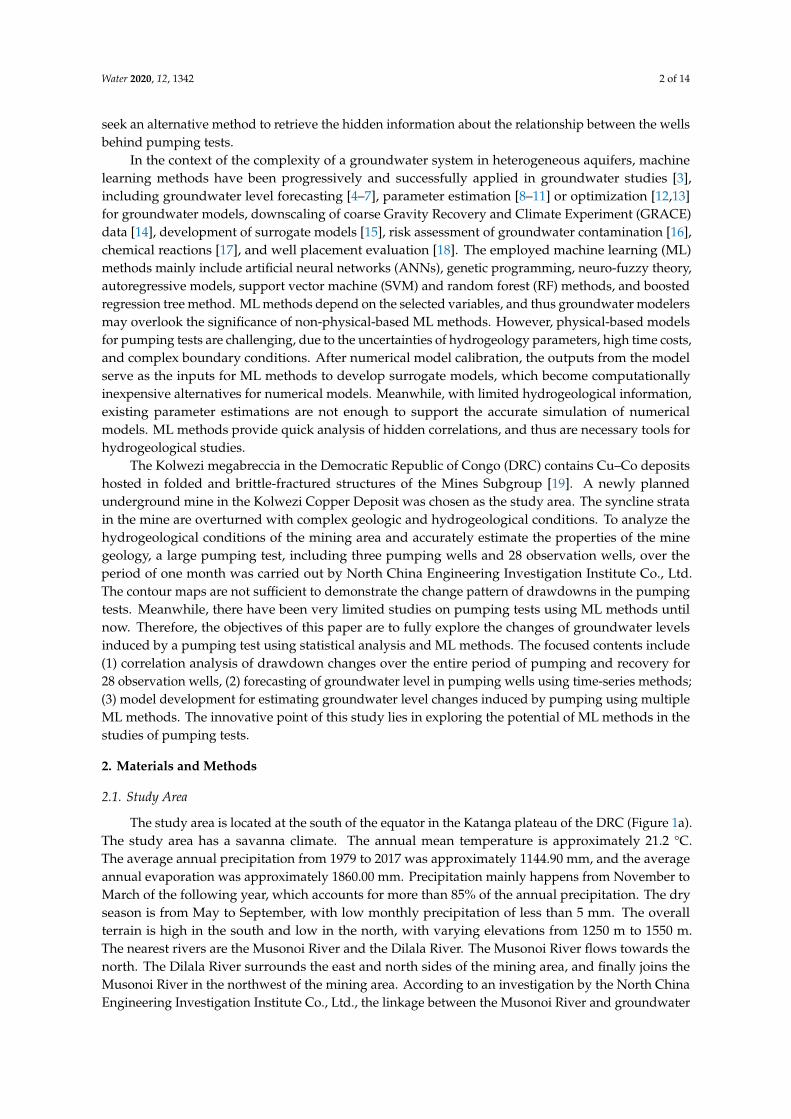
The strata in the study area are of the Late Proterozoic Katanga supergroup, which can be subdivided into the upper Kundelungu group and the lower Roan group (host strata). The strata in this area are mainly the Katanga series and the quaternary. The Katanga series mainly includes the Roan group (R), the Nguba group (Ng), and the Kundelungu group (Ku). A cross-section can be shown in Figure 1b [20]. The series of geology from young to old can be seen in Table 1. According to field investigation and regional studies, the average hydraulic conductivity of the Calcaire á Minerals Noirs (CMN) and the Roches Silicieuses Feuilletees (RSF) formations, where the breccia zones are developed, is approximately 0.65 m/d.

Figure 1. Location of the study area: (a) the geology and location of wells in the plain; (b) the geology along the cross-section line LL.

Table 1. List of regional stratigraphy in the study area.

Series (From Young to Old) Formation Local Name Brief Description

Approximated Thickness (m)

Kundelungu Kundelungu Ku Sediments 3000–5000 Nguba Nguba Ng Sandstone, shale 200–500

Upper Roan (R)

R4 Mwashya shale, siltstone, sandstone,

dolomites 50–100

R3-2 Dipeta Sandy shales about 1000 R3-1 Roches Greseuse Superior (RGS) Grey shales 100~200

Lower Roan

R2-3

Mines Group

Calcaire á Minerals Noirs (CMN) Black calcareous siltstone 130

R2-2 Schistes Dolomitic Superior (SDS) Dolomitic shales, black ore

mineral zone (BOMZ) 50–80

R2-1

Schistes de Base (SDB) Dolomitic shales, black ore

mineral zone (BOMZ) 10–15

Roches Silicieuses Cellulaire (RSC) Siliceous, vuggy dolomite 12–25 Roches Silicieuses Feuilletees (RSF) Bedded dolomitic siltstone 5

Dolomie Stratifiee (DSTRAT) Grey talcose sandstone 3 Roches Argileuses Talceuse (RAT) GRISES Grey talcose sandstone 2–5

R1 Roches Argileuses Talceuse (RAT2) Talcose sandstone 190 Roches Argileuses Talceuse (RAT1) Talcose sandstone 40

2.2. Pumping Tests

Figure 1. Location of the study area: (a) the geology and location of wells in the plain; (b) the geologyalong the cross-section line LL.

The strata in the study area are of the Late Proterozoic Katanga supergroup, which can besubdivided into the upper Kundelungu group and the lower Roan group (host strata). The stratain this area are mainly the Katanga series and the quaternary. The Katanga series mainly includesthe Roan group (R), the Nguba group (Ng), and the Kundelungu group (Ku). A cross-section can beshown in Figure 1b [20]. The series of geology from young to old can be seen in Table 1. According tofield investigation and regional studies, the average hydraulic conductivity of the Calcaire á MineralsNoirs (CMN) and the Roches Silicieuses Feuilletees (RSF) formations, where the breccia zones aredeveloped, is approximately 0.65 m/d.

2.2. Pumping Tests

Pumping tests were carried out from 8:00 a.m. on 22 November 2018 to 8:00 p.m. on 23 December 2018,which is almost 32 days. There were three pumping wells (P01, P02, and P03) and the productions ofeach pumping well were 1232.40, 3532.32, and 2790.64 m3/d, respectively (Figure 1a). The pumpingrates were changed to 0 at 8:00 a.m. on December 18, 2018, which means that groundwater level willgradually recover. During the period of pumping tests, the average precipitation was about 2.70 mmper day (Figure 2). There were 28 observation wells (including three pumping wells) in the mine area.The observed maximum drawdown among the wells was approximately 61 m in well P01, 58 m in wellP03, and 45 m in well P02, respectively. The location, the well depth, and the maximum drawdown ofeach well are listed in Table 2, and all wells are multilayered. The depths of well O12 and O24 are shallow,and changes of groundwater levels are subject to precipitation rather than pumping.

Water 2020, 12, 1342 4 of 14

Table 1. List of regional stratigraphy in the study area.

Series(From Young

to Old)Formation Local Name Brief Description Approximated

Thickness (m)

Kundelungu Kundelungu Ku Sediments 3000–5000

Nguba Nguba Ng Sandstone, shale 200–500

Upper Roan (R)

R4 Mwashya shale, siltstone,sandstone, dolomites 50–100

R3-2 Dipeta Sandy shales about 1000

R3-1Roches GreseuseSuperior (RGS) Grey shales 100–200

Lower Roan

R2-3

Mines Group

Calcaire á MineralsNoirs (CMN)

Black calcareoussiltstone 130

R2-2Schistes Dolomitic

Superior (SDS)

Dolomitic shales,black ore mineral

zone (BOMZ)50–80

R2-1

Schistes deBase (SDB)

Dolomitic shales,black ore mineral

zone (BOMZ)10–15

Roches SilicieusesCellulaire (RSC)

Siliceous,vuggy dolomite 12–25

Roches SilicieusesFeuilletees (RSF)

Bedded dolomiticsiltstone 5

Dolomie Stratifiee(DSTRAT)

Grey talcosesandstone 3

Roches ArgileusesTalceuse (RAT)

GRISES

Grey talcosesandstone 2–5

R1

Roches ArgileusesTalceuse (RAT2) Talcose sandstone 190

Roches ArgileusesTalceuse (RAT1) Talcose sandstone 40

Water 2020, 12, x FOR PEER REVIEW 4 of 14

Pumping tests were carried out from 8:00 a.m. on 22 November 2018 to 8:00 p.m. on 23 December 2018, which is almost 32 days. There were three pumping wells (P01, P02, and P03) and the productions of each pumping well were 1232.40, 3532.32, and 2790.64 m3/d, respectively (Figure 1a). The pumping rates were changed to 0 at 8:00 a.m. on December 18, 2018, which means that groundwater level will gradually recover. During the period of pumping tests, the average precipitation was about 2.70 mm per day (Figure 2). There were 28 observation wells (including three pumping wells) in the mine area. The observed maximum drawdown among the wells was approximately 61 m in well P01, 58 m in well P03, and 45 m in well P02, respectively. The location, the well depth, and the maximum drawdown of each well are listed in Table 2, and all wells are multilayered. The depths of well O12 and O24 are shallow, and changes of groundwater levels are subject to precipitation rather than pumping.

Figure 2. Change of precipitation over the entire pumping test.

Table 2. List of the location, depth, and maximum drawdown of wells.

ID Well Name X Coordinate (m)

Y Coordinate (m)

Well Depth (m)

Maximum Drawdown (m)

1 P01 332,585.13 8,817,317.16 310.20 61.21 2 P02 332,754.99 8,817,435.06 251.51 45.08 3 P03 332,259.70 8,817,203.31 325.00 57.70 4 O01 332,466.69 8,817,664.79 110.39 0.42 5 O02 332,522.15 8,817,498.36 300.20 1.22 6 O03 332,061.84 8,817,135.65 330.19 22.35 7 O04 331,489.21 8,816,936.91 150.56 1.39 8 O05 333,045.08 8,817,509.79 300.05 7.55 9 O06 333,190.69 8,817,610.82 110.03 0.59

10 O07 332,821.69 8,816,666.56 150.95 0.27 11 O08 332,805.85 8,816,292.67 102.25 0.15 12 O09 330,946.09 8,817,636.84 100.25 0.13 13 O10 331,761.74 8,817,414.28 100.42 0.68 14 O11 330,483.97 8,817,678.42 150.00 0.48 15 O12 330,483.97 8,817,678.42 50.00 −0.13 16 O13 332,594.98 8,817,275.07 400.07 18.16 17 O14 332,856.15 8,817,437.12 344.13 37.27 18 O15 332,253.28 8,817,166.53 324.75 27.81 19 O16 332,709.88 8,817,245.02 450.20 3.84 20 O17 332,475.42 8,817,329.49 330.51 18.20 21 O18 332,546.68 8,817,209.31 602.00 2.94 22 O19 332,442.94 8,817,113.78 658.00 1.81 23 O20 332,778.77 8,817,213.32 346.00 4.86 24 O21 332,735.77 8,817,305.28 442.00 4.38 25 O22 332,515.40 8,817,012.31 612.00 2.26 26 O23 331,833.07 8,816,934.75 281.05 3.01

Figure 2. Change of precipitation over the entire pumping test.

Water 2020, 12, 1342 5 of 14

Table 2. List of the location, depth, and maximum drawdown of wells.

ID Well Name X Coordinate(m)

Y Coordinate(m)

Well Depth(m)

Maximum Drawdown(m)

1 P01 332,585.13 8,817,317.16 310.20 61.212 P02 332,754.99 8,817,435.06 251.51 45.083 P03 332,259.70 8,817,203.31 325.00 57.704 O01 332,466.69 8,817,664.79 110.39 0.425 O02 332,522.15 8,817,498.36 300.20 1.226 O03 332,061.84 8,817,135.65 330.19 22.357 O04 331,489.21 8,816,936.91 150.56 1.398 O05 333,045.08 8,817,509.79 300.05 7.559 O06 333,190.69 8,817,610.82 110.03 0.59

10 O07 332,821.69 8,816,666.56 150.95 0.2711 O08 332,805.85 8,816,292.67 102.25 0.1512 O09 330,946.09 8,817,636.84 100.25 0.1313 O10 331,761.74 8,817,414.28 100.42 0.6814 O11 330,483.97 8,817,678.42 150.00 0.4815 O12 330,483.97 8,817,678.42 50.00 −0.1316 O13 332,594.98 8,817,275.07 400.07 18.1617 O14 332,856.15 8,817,437.12 344.13 37.2718 O15 332,253.28 8,817,166.53 324.75 27.8119 O16 332,709.88 8,817,245.02 450.20 3.8420 O17 332,475.42 8,817,329.49 330.51 18.2021 O18 332,546.68 8,817,209.31 602.00 2.9422 O19 332,442.94 8,817,113.78 658.00 1.8123 O20 332,778.77 8,817,213.32 346.00 4.8624 O21 332,735.77 8,817,305.28 442.00 4.3825 O22 332,515.40 8,817,012.31 612.00 2.2626 O23 331,833.07 8,816,934.75 281.05 3.0127 O24 332,026.27 8,816,985.75 50.00 −0.1728 O25 332,026.27 8,816,985.75 150.00 8.95

2.3. Methods

The methods used in this paper include Pearson correlation analysis, k-means clustering, and MLmodels consisting of autoregressive integrated moving average (ARIMA) [21], ANN [22], support vectormachine (SVR) [23], and RF [4] methods. These methods are applied using Python language [24,25].

2.3.1. Pearson Correlation Analysis

The correlation of time-series groundwater level data between pumping wells and observationwells will be analyzed. The Pearson correlation coefficient used here is usually applicable to calculatethe relationships between two time series, X(t) and Y(t) (t = 1, 2, 3, . . . n), and can be expressed as

PR(X, Y) =Cov(X(t), Y(t))√

Var[X(t)]Var[Y(t)](1)

where PR is the Pearson correlation coefficient; Cov is covariance, Var is variance, n is number ofobservation data, and t is time period.

2.3.2. Cluster Analysis

After the Pearson correlation coefficient between two wells are obtained, k-means clusteringalgorithms are adopted to further study the relationship of drawdowns in wells, which partitions thedata space into Voronoi cell representations. This transformation divides the data observations intok-clusters. in which each of the observations belongs to the cluster with the nearest mean. Being in thesame cluster means the wells have similar hydraulic properties.

Water 2020, 12, 1342 6 of 14

2.3.3. Time-Series Analysis Method of Drawdowns within Pumping Wells

For the pumping tests, groundwater level changes within the three pumping wells were directresponses to the groundwater pumping, and groundwater levels at other observation wells wereinduced by groundwater pumping. Because the pumping rates of three pumping wells are constant,drawdowns within three pumping wells are selected as the independent variable. The autoregressiveintegrated moving average (ARIMA) method was adopted here to forecast the changes of groundwaterlevels within the three pumping wells; thus, the results can be used to predict the changes of drawdownsin other observation wells. The ARIMA model consists of an autoregressive (AR) model, movingaverage (MA) model, and differencing method to make the time series stationary. The (p,d,q) order of themodel is the number of AR parameters, differences, and MA parameters in the model, respectively. First,the differential order is determined by the try-and-error method, and an augmented Dickey–Fuller testis performed to check whether the differential time series is stationary. Then the order of autoregressionand moving average will be given from the changes in the time-series data. Then the established ARIMAmodel will be trained and used to predict the changes of groundwater levels. Finally, differentialreduction of the predicted results will be performed to get final simulated results.

2.3.4. Forecasting Method for Groundwater Levels among Observation Wells

When groundwater levels within pumping wells are predicted, other observation well data canbe estimated by the relationships between water levels of the observation wells, water levels of thethree pumping wells, and changes of precipitation in this region. The relationships will be establishedby three widely used ML methods: ANN, SVR, and RF. The model evaluation criteria was carried outby the root mean square error (RMSE) between the observed and simulated time-series data, as

RMSE =

√√1n

n∑t=1

(X(t) −Y(t))2 (2)

where X(t) is the reference-measured dataset; Y(t) is the modeled dataset from ANN, SVR, and RFmethods; and n is the total number of observations.

2.3.5. Linear Graphic Method in the Theis Model

The linear graphic method in the Theis model is used to estimate the value of hydraulic conductivity.When the pumping duration is large enough, the drawdowns can be expressed using Equation (3).When the plot of the drawdowns and the logarithm time is drawn, the slope will be easily obtained bylinear regressive method, and then hydraulic conductivity can be estimated when the pumping rateand the thickness of the aquifer are known:

s =Q

4πKMW(

Kr2

4Syt) ≈ 0.183

QKM

lg2.25KSyr2 + 0.183

QKM

lgt (3)

where s is the drawdown, Q is the pumping rate, K is hydraulic conductivity, Sy is storativity, r is theradial distance from the observation well to the pumping well, and t is pumping duration.

3. Results

3.1. Distribution of Maximum Drawdown

Although the multilayered observation wells are not at the same depths as the boreholes,the contour map of maximum drawdowns for all wells is firstly projected in the same plain.From Figure 3, the distribution of maximum drawdown is highly uniform. The long axis of themaximum drawdown is approximately 45◦ northeast, and the length of the influence is approximately

Water 2020, 12, 1342 7 of 14

1.50 km. The short axis of maximum drawdown is approximately 45◦ northwest, and the length of theinfluence is approximately 1.0 km.

Water 2020, 12, x FOR PEER REVIEW 6 of 14

( )2

1

1 ( ) ( )n

tRMSE X t Y t

n =

= −

(2)

where ( )X t is the reference-measured dataset; ( )Y t is the modeled dataset from ANN, SVR, and RF methods; and n is the total number of observations.

2.3.5. Linear Graphic Method in the Theis Model

The linear graphic method in the Theis model is used to estimate the value of hydraulic conductivity. When the pumping duration is large enough, the drawdowns can be expressed using Equation (3). When the plot of the drawdowns and the logarithm time is drawn, the slope will be easily obtained by linear regressive method, and then hydraulic conductivity can be estimated when the pumping rate and the thickness of the aquifer are known:

tKM

Q

rS

K

KM

Q

tS

KrW

KM

Qs

yy

lg183.025.2

lg183.0)4

(4 2

2

+≈=π

(3)

where s is the drawdown, Q is the pumping rate, K is hydraulic conductivity, Sy is storativity, r is the radial distance from the observation well to the pumping well, and t is pumping duration.

3. Results

3.1. Distribution of Maximum Drawdown

Although the multilayered observation wells are not at the same depths as the boreholes, the contour map of maximum drawdowns for all wells is firstly projected in the same plain. From Figure 3, the distribution of maximum drawdown is highly uniform. The long axis of the maximum drawdown is approximately 45° northeast, and the length of the influence is approximately 1.50 km. The short axis of maximum drawdown is approximately 45º northwest, and the length of the influence is approximately 1.0 km.

Figure 3. Contour map of maximum drawdown in the Musonoi mine area.

3.2. Relationship of Water Levels between Observation and Pumping Wells

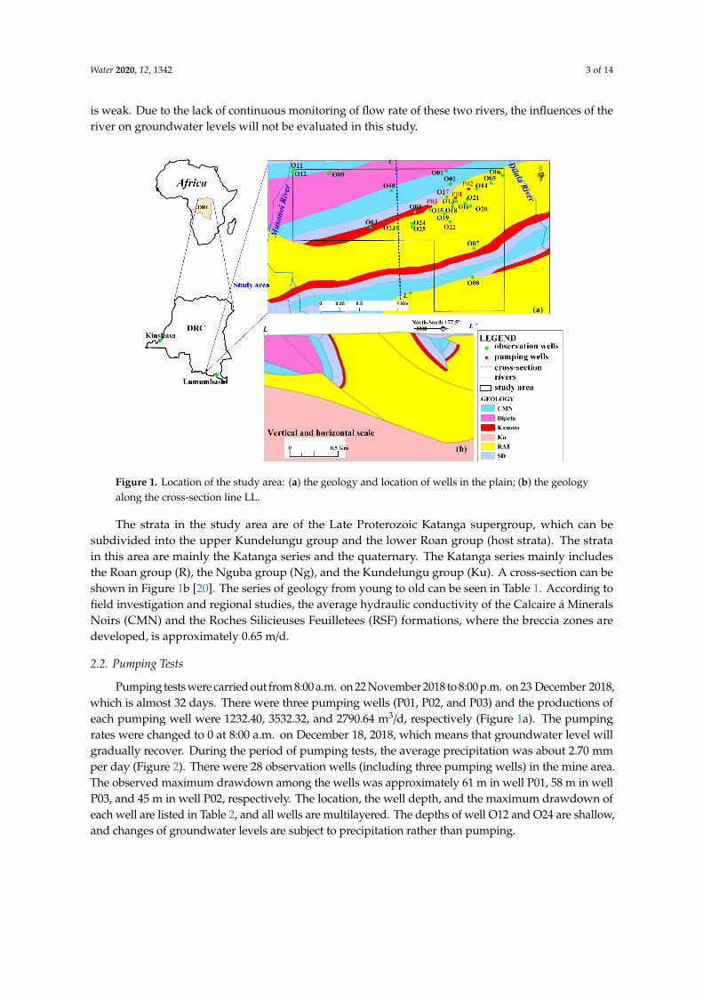
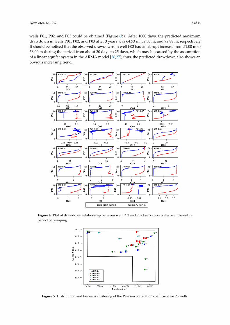
Pumping well P03 is located almost at the center of the study area, with considerable pumping rates, and was thus chosen as a representative pumping well to demonstrate relationships with other wells. The relationship over the pumping period (blue line) and the restoring period (red line) between well P03 and other wells are shown in Figure 4. K-means clustering of the Pearson correlation coefficient (PR) for 28 observation wells (Figure 5) is drawn to clarify the relationship. Four clusters (clusters #1, #2, #3, and #4) are divided based on the value of the Pearson correlation

Figure 3. Contour map of maximum drawdown in the Musonoi mine area.

3.2. Relationship of Water Levels between Observation and Pumping Wells

Pumping well P03 is located almost at the center of the study area, with considerable pumpingrates, and was thus chosen as a representative pumping well to demonstrate relationships with otherwells. The relationship over the pumping period (blue line) and the restoring period (red line) betweenwell P03 and other wells are shown in Figure 4. K-means clustering of the Pearson correlation coefficient(PR) for 28 observation wells (Figure 5) is drawn to clarify the relationship. Four clusters (clusters #1,#2, #3, and #4) are divided based on the value of the Pearson correlation coefficient. The first cluster(cluster #1) includes observation wells P01, P02, P03, O13, O14, O15, O17, and O01, which have thehigher PR (over 0.75) with pumping well P03. The second cluster (cluster #2) consists of wells O03,O18, O19, O21, O04, O06, O11, O07, and O08, with the correlation ranging from 0.44 to 0.64. The PR inthe third cluster (cluster #3) for observation wells O02, O10, O16, O24, and O09 varied from 0.16 to0.32. Observation wells O23, O25, O22, O20, O05, and O12 are attributed to the fourth cluster (cluster#4), with a PR less than 0.10. Observation wells with higher PR values basically surrounded the threepumping wells. It should be noticed that observation wells with relatively higher PR values (cluster#2) did not always surround three pumping wells. For example, wells O11 and O08 are a little fartheraway from the pumping wells; observation wells for cluster #3 and #4 are progressively farther awayfrom the pumping wells. The high PR value suggests that the hydraulic connections for the wells incluster #1 are perfect.

3.3. Predictions of Drawdowns within Pumping Wells

Drawdowns within pumping wells are direct responses of groundwater pumping. Under thecondition of a constant pumping rate, drawdowns within wells will be progressively increased.The ARIMA method is used to predict the change of the drawdown. For validating the accuracyof the ARIMA model, a hypothetical confined aquifer satisfying the Theis model is first established.Any parameters in the Theis model can be assumed. Pumping rate, the thickness of the aquifer,hydraulic conductivities, storativities, and the radial distance away from the pumping well in theTheis model for an observation well is set as 100.00 m3/d, 20.00 m, 0.50 m/d, 10−6 m−1, and 5.00 m,respectively. The relative error, defined as the ratio of the absolute error between the simulated andanalytical drawdowns to the analytical solutions, was only 0.86% after about 1.37 × 109 years ofpumping for the hypothetical Theis model (Figure 6a), suggesting that the ARIMA method can be usedto accurately predict changes of the drawdown with time. After making the time series stationary andtraining the ARIMA model with a p-value less than 10−3, changes of the drawdown in three pumping

Water 2020, 12, 1342 8 of 14

wells P01, P02, and P03 could be obtained (Figure 6b). After 1000 days, the predicted maximumdrawdown in wells P01, P02, and P03 after 3 years was 64.53 m, 52.50 m, and 92.88 m, respectively.It should be noticed that the observed drawdowns in well P03 had an abrupt increase from 51.00 m to56.00 m during the period from about 20 days to 25 days, which may be caused by the assumptionof a linear aquifer system in the ARMA model [26,27]; thus, the predicted drawdown also shows anobvious increasing trend.

Water 2020, 12, x FOR PEER REVIEW 7 of 14

coefficient. The first cluster (cluster #1) includes observation wells P01, P02, P03, O13, O14, O15, O17, and O01, which have the higher PR (over 0.75) with pumping well P03. The second cluster (cluster #2) consists of wells O03, O18, O19, O21, O04, O06, O11, O07, and O08, with the correlation ranging from 0.44 to 0.64. The PR in the third cluster (cluster #3) for observation wells O02, O10, O16, O24, and O09 varied from 0.16 to 0.32. Observation wells O23, O25, O22, O20, O05, and O12 are attributed to the fourth cluster (cluster #4), with a PR less than 0.10. Observation wells with higher PR values basically surrounded the three pumping wells. It should be noticed that observation wells with relatively higher PR values (cluster #2) did not always surround three pumping wells. For example, wells O11 and O08 are a little farther away from the pumping wells; observation wells for cluster #3 and #4 are progressively farther away from the pumping wells. The high PR value suggests that the hydraulic connections for the wells in cluster #1 are perfect.

Figure 4. Plot of drawdown relationship between well P03 and 28 observation wells over the entire period of pumping. Figure 4. Plot of drawdown relationship between well P03 and 28 observation wells over the entireperiod of pumping.

Water 2020, 12, x FOR PEER REVIEW 8 of 14

Figure 5. Distribution and k-means clustering of the Pearson correlation coefficient for 28 wells.

3.3. Predictions of Drawdowns within Pumping Wells

Drawdowns within pumping wells are direct responses of groundwater pumping. Under the condition of a constant pumping rate, drawdowns within wells will be progressively increased. The ARIMA method is used to predict the change of the drawdown. For validating the accuracy of the ARIMA model, a hypothetical confined aquifer satisfying the Theis model is first established. Any parameters in the Theis model can be assumed. Pumping rate, the thickness of the aquifer, hydraulic conductivities, storativities, and the radial distance away from the pumping well in the Theis model for an observation well is set as 100.00 m3/d, 20.00 m, 0.50 m/d, 10−6 m–1, and 5.00 m, respectively. The relative error, defined as the ratio of the absolute error between the simulated and analytical drawdowns to the analytical solutions, was only 0.86% after about 1.37 × 109 years of pumping for the hypothetical Theis model (Figure 6a), suggesting that the ARIMA method can be used to accurately predict changes of the drawdown with time. After making the time series stationary and training the ARIMA model with a p-value less than 10–3, changes of the drawdown in three pumping wells P01, P02, and P03 could be obtained (Figure 6b). After 1000 days, the predicted maximum drawdown in wells P01, P02, and P03 after 3 years was 64.53 m, 52.50 m, and 92.88 m, respectively. It should be noticed that the observed drawdowns in well P03 had an abrupt increase from 51.00 m to 56.00 m during the period from about 20 days to 25 days, which may be caused by the assumption of a linear aquifer system in the ARMA model [26,27]; thus, the predicted drawdown also shows an obvious increasing trend.

(a)

(b)

Figure 6. Train and forecast of drawdowns within pumping wells, (a) the Theis model; (b) the autoregressive integrated moving average (ARIMA) model.

Figure 5. Distribution and k-means clustering of the Pearson correlation coefficient for 28 wells.

Water 2020, 12, 1342 9 of 14

Water 2020, 12, x FOR PEER REVIEW 8 of 14

Figure 5. Distribution and k-means clustering of the Pearson correlation coefficient for 28 wells.

3.3. Predictions of Drawdowns within Pumping Wells

Drawdowns within pumping wells are direct responses of groundwater pumping. Under the condition of a constant pumping rate, drawdowns within wells will be progressively increased. The ARIMA method is used to predict the change of the drawdown. For validating the accuracy of the ARIMA model, a hypothetical confined aquifer satisfying the Theis model is first established. Any parameters in the Theis model can be assumed. Pumping rate, the thickness of the aquifer, hydraulic conductivities, storativities, and the radial distance away from the pumping well in the Theis model for an observation well is set as 100.00 m3/d, 20.00 m, 0.50 m/d, 10−6 m–1, and 5.00 m, respectively. The relative error, defined as the ratio of the absolute error between the simulated and analytical drawdowns to the analytical solutions, was only 0.86% after about 1.37 × 109 years of pumping for the hypothetical Theis model (Figure 6a), suggesting that the ARIMA method can be used to accurately predict changes of the drawdown with time. After making the time series stationary and training the ARIMA model with a p-value less than 10–3, changes of the drawdown in three pumping wells P01, P02, and P03 could be obtained (Figure 6b). After 1000 days, the predicted maximum drawdown in wells P01, P02, and P03 after 3 years was 64.53 m, 52.50 m, and 92.88 m, respectively. It should be noticed that the observed drawdowns in well P03 had an abrupt increase from 51.00 m to 56.00 m during the period from about 20 days to 25 days, which may be caused by the assumption of a linear aquifer system in the ARMA model [26,27]; thus, the predicted drawdown also shows an obvious increasing trend.

(a)

(b)

Figure 6. Train and forecast of drawdowns within pumping wells, (a) the Theis model; (b) the autoregressive integrated moving average (ARIMA) model.

Figure 6. Train and forecast of drawdowns within pumping wells, (a) the Theis model; (b) theautoregressive integrated moving average (ARIMA) model.

3.4. Predictions of Drawdowns in Observation Wells

The pumping tests here were carried out in the period from the dry season to the wet season. As aresult, changes of the drawdown in observation wells were mainly subject to the combined influencesof precipitation conditions, the pumping rate of three wells, and aquifer properties. Independentvariables include the precipitation and the drawdown in three pumping wells. The dependent variableis the drawdown for each observation well. The ANN, RF, and SVR methods were all applied topredict the drawdowns for 25 observation wells. Both the first and second hidden layer of the ANNmodel were set as 10, the number of trees in the RF method was set at 500, the radial basis function (rbf )was used as the kernel function of the SVR model, and the regularization parameter c was set as 10,000.Changes in simulated drawdowns over time from ANN, RF, and SVR methods are shown in Figure 7.All three methods can simulate the trend of groundwater level changes well. The average RMSEvalue for the 25 observation wells for the ANN, RF, and SVR methods is 0.51 m, 0.13 m, and 0.13 m,respectively, suggesting that the RF and SVR methods show relatively better results than the ANNmethod. Li et al. [28] applied RF, ANN, and SVM to forecast lake water level variations, and also foundthe RF model exhibits the best performance, which is consist with the findings in this study.

Water 2020, 12, x FOR PEER REVIEW 9 of 14

3.4. Predictions of Drawdowns in Observation Wells

The pumping tests here were carried out in the period from the dry season to the wet season. As a result, changes of the drawdown in observation wells were mainly subject to the combined influences of precipitation conditions, the pumping rate of three wells, and aquifer properties. Independent variables include the precipitation and the drawdown in three pumping wells. The dependent variable is the drawdown for each observation well. The ANN, RF, and SVR methods were all applied to predict the drawdowns for 25 observation wells. Both the first and second hidden layer of the ANN model were set as 10, the number of trees in the RF method was set at 500, the radial basis function (rbf) was used as the kernel function of the SVR model, and the regularization parameter c was set as 10,000. Changes in simulated drawdowns over time from ANN, RF, and SVR methods are shown in Figure 7. All three methods can simulate the trend of groundwater level changes well. The average RMSE value for the 25 observation wells for the ANN, RF, and SVR methods is 0.51 m, 0.13 m, and 0.13 m, respectively, suggesting that the RF and SVR methods show relatively better results than the ANN method. Li et al. [28] applied RF, ANN, and SVM to forecast lake water level variations, and also found the RF model exhibits the best performance, which is consist with the findings in this study.

Figure 7. Changes of the simulated drawdowns with time from artificial neural network (ANN), random forest (RF), and support vector machine (SVR) methods for 25 observation wells.

4. Discussion

As discussed earlier, the PR coefficient only demonstrates the relationship of groundwater level changes for two wells. The k-means cluster using three variables (PR coefficient, drawdown, and well depth) is further divided to find the hydraulic connections between these wells. It can be clearly observed from Figure 8a that cluster #1 (wells P01, P02, P03, O02, O03, O05, O14, O15, O17, O20, and O23) is located at a depth ranging from 250 m to 350 m, suggesting the hydraulic connection are perfect at such a depth. The clustering was projected to a two-dimensional (2D) map (Figure 8b), and it was found that the axis of maximum drawdown was along the line AA’ from the southwest to the northeast. Furthermore, the drawdown south of line AA’ is better than that north of the line, which is importantly caused by the fact that the existing syncline, which makes an aquifer with perfect

Figure 7. Changes of the simulated drawdowns with time from artificial neural network (ANN),random forest (RF), and support vector machine (SVR) methods for 25 observation wells.

Water 2020, 12, 1342 10 of 14

4. Discussion

As discussed earlier, the PR coefficient only demonstrates the relationship of groundwater levelchanges for two wells. The k-means cluster using three variables (PR coefficient, drawdown, and welldepth) is further divided to find the hydraulic connections between these wells. It can be clearlyobserved from Figure 8a that cluster #1 (wells P01, P02, P03, O02, O03, O05, O14, O15, O17, O20,and O23) is located at a depth ranging from 250 m to 350 m, suggesting the hydraulic connectionare perfect at such a depth. The clustering was projected to a two-dimensional (2D) map (Figure 8b),and it was found that the axis of maximum drawdown was along the line AA’ from the southwestto the northeast. Furthermore, the drawdown south of line AA’ is better than that north of the line,which is importantly caused by the fact that the existing syncline, which makes an aquifer with perfectpermeability, extends from the northwest to the southeast (Figure 1b), and thus the permeability at thesoutheastern part is better than that in the northwest.

Water 2020, 12, x FOR PEER REVIEW 10 of 14

permeability, extends from the northwest to the southeast (Figure 1b), and thus the permeability at the southeastern part is better than that in the northwest.

(a)

(b)

Figure 8. Schematic figures of the k-means clustering demonstrated in three-dimensional (3D) and two-dimensional (2D) space using the PR coefficient, drawdown, and well depth. (a) 3D space, (b) 2D space.

Established ANN, SVR, and RF models can accurately predict the change of the drawdown for 25 observation wells; however, the parameters in these models may have certain influences on the model results. Well O15 with big drawdowns (cluster #1) and well O19 with small drawdowns (cluster #2) were selected to evaluate the influences of parameters on model results. Table 3 lists the value of parameters, RMSE, and average relative errors in the three models for wells O15 and O19. The relative error here is defined as the average ratio of absolute error between simulated and observed drawdown to the observed drawdown for all observed results.

Table 3. List of root mean square error (RMSE) values and average relative error in ANN, SVR, and RF methods for wells O15 and O19.

Models Parameters RMSE (m) Average Relative

Error (%)

Well O15 Well O19 Well O15

Well O19

ANN Model number of the first and the second hidden layers

(2, 2) 5.1972 0.3516 90.64 220.01 (5, 5) 0.8717 0.1834 9.66 195.83

(10, 10) 0.5844 0.1998 16.30 84.34 (100, 100) 0.5085 0.1237 10.56 89.60

SVR Model kernel function (the radial

basis function (rbf) and linear) and parameter c

rbf, c = 10 1.1462 0.0941 76.40 96.87 rbf, c = 100 0.0926 0.0941 1.90 96.87

rbf, c = 1000 0.0926 0.0941 1.90 96.87 linear, c = 1000 2.6271 5.4130 58.95 2443.24

RF Model number of trees (n)

n = 5 0.2429 0.0551 14.13 22.01 n = 50 0.2071 0.0468 11.57 13.38 n = 500 0.1842 0.0416 11.17 14.84

n = 5000 0.1853 0.0394 10.91 15.17

Figure 9 reveals the influences of model parameters on model bias, which is the difference between the simulated and the observed drawdown. For the ANN model, with the increase of the hidden layers, the model bias will be gradually reduced, and when the number of the first and second hidden layers is over 5, RMSE is less than 0.88 m and 0.20 m for wells O15 and O19, respectively, but the average relative errors for well O15 and O19 are about 15% and 85%, respectively. For the SVR model, results using the rbf kernel function give better predictions than those using the linear kernel function, and the higher value of parameter c will improve the accuracy of the models. However,

Figure 8. Schematic figures of the k-means clustering demonstrated in three-dimensional (3D) andtwo-dimensional (2D) space using the PR coefficient, drawdown, and well depth. (a) 3D space,(b) 2D space.

Established ANN, SVR, and RF models can accurately predict the change of the drawdown for25 observation wells; however, the parameters in these models may have certain influences on themodel results. Well O15 with big drawdowns (cluster #1) and well O19 with small drawdowns (cluster#2) were selected to evaluate the influences of parameters on model results. Table 3 lists the value ofparameters, RMSE, and average relative errors in the three models for wells O15 and O19. The relativeerror here is defined as the average ratio of absolute error between simulated and observed drawdownto the observed drawdown for all observed results.

Figure 9 reveals the influences of model parameters on model bias, which is the difference betweenthe simulated and the observed drawdown. For the ANN model, with the increase of the hidden layers,the model bias will be gradually reduced, and when the number of the first and second hidden layersis over 5, RMSE is less than 0.88 m and 0.20 m for wells O15 and O19, respectively, but the averagerelative errors for well O15 and O19 are about 15% and 85%, respectively. For the SVR model, resultsusing the rbf kernel function give better predictions than those using the linear kernel function, and thehigher value of parameter c will improve the accuracy of the models. However, when the value of c isgreater than 100, the models with the rbf kernel function results are not improved significantly forwells O15 and O19, with RMSEs over 0.53 m (average relative error about 1.90%) and 1.08 m (averagerelative error about 96.87%), respectively. Meanwhile, the change of the drawdown for well O19 wasless sensitive to the parameter c than that for well O15. The sensitivities to parameters in the RF modelfor both well O15 and well O19 were less than those from the ANN and SVR models: RMSE valueswere about 0.18–0.25 m, with a relative error about 11.00–14.00% for well O15, and 0.039–0.055 m,with average relative error about 13.38–22.01% for well O19. Considering RMSE and average relative

Water 2020, 12, 1342 11 of 14

error, the RF model gives the most accurate results and has fewer sensitivities to parameters; thus,is the most appropriate model in this study.

Table 3. List of root mean square error (RMSE) values and average relative error in ANN, SVR, and RFmethods for wells O15 and O19.

Models ParametersRMSE (m) Average Relative Error (%)

Well O15 Well O19 Well O15 Well O19

ANN Modelnumber of the first

and the secondhidden layers

(2, 2) 5.1972 0.3516 90.64 220.01

(5, 5) 0.8717 0.1834 9.66 195.83

(10, 10) 0.5844 0.1998 16.30 84.34

(100, 100) 0.5085 0.1237 10.56 89.60

SVR Model

kernel function(the radial basis

function (rbf ) andlinear) andparameter c

rbf, c = 10 1.1462 0.0941 76.40 96.87

rbf, c = 100 0.0926 0.0941 1.90 96.87

rbf, c = 1000 0.0926 0.0941 1.90 96.87

linear, c = 1000 2.6271 5.4130 58.95 2443.24

RF Model number of trees (n)

n = 5 0.2429 0.0551 14.13 22.01

n = 50 0.2071 0.0468 11.57 13.38

n = 500 0.1842 0.0416 11.17 14.84

n = 5000 0.1853 0.0394 10.91 15.17

Water 2020, 12, x FOR PEER REVIEW 11 of 14

when the value of c is greater than 100, the models with the rbf kernel function results are not improved significantly for wells O15 and O19, with RMSEs over 0.53 m (average relative error about 1.90%) and 1.08 m (average relative error about 96.87%), respectively. Meanwhile, the change of the drawdown for well O19 was less sensitive to the parameter c than that for well O15. The sensitivities to parameters in the RF model for both well O15 and well O19 were less than those from the ANN and SVR models: RMSE values were about 0.18–0.25 m, with a relative error about 11.00–14.00% for well O15, and 0.039–0.055 m, with average relative error about 13.38–22.01% for well O19. Considering RMSE and average relative error, the RF model gives the most accurate results and has fewer sensitivities to parameters; thus, is the most appropriate model in this study.

Figure 9. Influence of parameters in ANN, SVR, and RF models on the simulated drawdowns for wells O15 and O19: (a, b, c) represent the results from ANN, SVR, and RF methods for well O15, respectively; (d, e, f) represent the results from ANN, SVR, and RF methods for well O19, respectively.

One of the important objectives of pumping tests is to estimate aquifer properties. ML methods lack the mechanics of groundwater flow, and cannot directly estimate hydraulic conductivity like analytical solutions. From the Theis model, the relationship between the drawdown and the logarithm time since the start of pumping become linear when time is long enough and the model satisfies the assumption of a Theis model. Therefore, wells O15, O03, O23, O19, O16, O20, and O11, which had relatively higher PR coefficients with the pumping rates, were chosen to establish the linear regressive model (Figure 10). The slope of the linear regressive model has a negative relationship with the value of the hydraulic conductivity, and thus can be used to estimate the hydraulic conductivity like the Theis model. Well O03 had the highest slope (almost 10), and estimated average hydraulic conductivity from well P03 to O03 was about 0.15 m/d, given that the pumping rate was about 2800 m3/d and the average aquifer thickness was about 330 m. It was noticed

Figure 9. Influence of parameters in ANN, SVR, and RF models on the simulated drawdowns for wellsO15 and O19: (a–c) represent the results from ANN, SVR, and RF methods for well O15, respectively;(d–f) represent the results from ANN, SVR, and RF methods for well O19, respectively.

Water 2020, 12, 1342 12 of 14

One of the important objectives of pumping tests is to estimate aquifer properties. ML methodslack the mechanics of groundwater flow, and cannot directly estimate hydraulic conductivity likeanalytical solutions. From the Theis model, the relationship between the drawdown and the logarithmtime since the start of pumping become linear when time is long enough and the model satisfies theassumption of a Theis model. Therefore, wells O15, O03, O23, O19, O16, O20, and O11, which hadrelatively higher PR coefficients with the pumping rates, were chosen to establish the linear regressivemodel (Figure 10). The slope of the linear regressive model has a negative relationship with the valueof the hydraulic conductivity, and thus can be used to estimate the hydraulic conductivity like the Theismodel. Well O03 had the highest slope (almost 10), and estimated average hydraulic conductivity fromwell P03 to O03 was about 0.15 m/d, given that the pumping rate was about 2800 m3/d and the averageaquifer thickness was about 330 m. It was noticed that well O11 had the lowest slope (about 0.21) andwas the furthest distance away from the pumping wells among these wells; in addition, the estimatedhydraulic conductivity may have reached about 7.00 m/d if the average aquifer thickness was set as350 m. The estimated average hydraulic conductivity for wells O13, O23, O19, O16, and O20 was about1.23 m/d, which is at the same magnitude as in previous studies (0.65 m/d) on this region.

Water 2020, 12, x FOR PEER REVIEW 12 of 14

that well O11 had the lowest slope (about 0.21) and was the furthest distance away from the pumping wells among these wells; in addition, the estimated hydraulic conductivity may have reached about 7.00 m/d if the average aquifer thickness was set as 350 m. The estimated average hydraulic conductivity for wells O13, O23, O19, O16, and O20 was about 1.23 m/d, which is at the same magnitude as in previous studies (0.65 m/d) on this region.

Figure 10. Relationship of drawdowns and time for wells O15, O03, O23, O19, O16, O20, and O11.

5. Conclusions

Pumping tests are very important means for investigating aquifer properties; however, common analytical solutions become invalid for interpreting the data when aquifers are anisotropic and heterogeneous. The paper explored the potential of ML methods for analyzing pumping test information in a field site. The study area is located at a mine area that has a pumping test with three pumping wells and 28 observation wells, over the period of about 32 days. Results found that ML methods can be successfully applied to simulate groundwater level changes induced by pumping and retrieve the relationship of groundwater levels between wells. Improving our understanding of pumping tests using ML methods requires (1) providing the fast and visual pictures of drawdowns between pumping wells and observation wells; (2) forecasting the changes of drawdowns in the observation wells, as well as in the pumping wells; (3) inferring the possible pathways of hydraulic connections in complex geology formations; (4) estimating average hydraulic conductivities. The main conclusions include:

(1) Rather than the mere contour map of the maximum drawdowns, the relationships of the drawdown over the period of pumping tests between wells provide a visual picture using ML methods, and the cluster of Pearson correlation coefficient shows the hydraulic connections between wells;

(2) The ARIMA method can be used to effectively predict the time-series changes of drawdowns in three pumping wells. In the hypothetical Theis model, the relative error of drawdowns is only 0.86% after 1.37 × 109 years. The predicted maximum drawdown in well P01, P02, and P03 after 3 years is 64.53 m, 52.50 m, and 92.88 m, respectively;

(3) Trained ANN, SVR, and RF models can reasonably capture the change of drawdowns in 25 observation wells induced by pumping; however, SVR and RF models provide better estimates, with average RMSE values for drawdowns of 0.13 m;

(4) K-means clustering using the Pearson correlation coefficient, the maximum drawdown, and well depth visually shows a preferable pathway, with the good permeability under depths ranging from 250 m to 350 m;

(5) Model parameters have certain influences on the simulated drawdowns for ANN, SVR, and RF models, but the RF model shows the least sensitivity to the value of the parameters, and has the best performance when compared with observed results;

Figure 10. Relationship of drawdowns and time for wells O15, O03, O23, O19, O16, O20, and O11.

5. Conclusions

Pumping tests are very important means for investigating aquifer properties; however, commonanalytical solutions become invalid for interpreting the data when aquifers are anisotropic andheterogeneous. The paper explored the potential of ML methods for analyzing pumping testinformation in a field site. The study area is located at a mine area that has a pumping test with threepumping wells and 28 observation wells, over the period of about 32 days. Results found that MLmethods can be successfully applied to simulate groundwater level changes induced by pumpingand retrieve the relationship of groundwater levels between wells. Improving our understanding ofpumping tests using ML methods requires (1) providing the fast and visual pictures of drawdownsbetween pumping wells and observation wells; (2) forecasting the changes of drawdowns in theobservation wells, as well as in the pumping wells; (3) inferring the possible pathways of hydraulicconnections in complex geology formations; (4) estimating average hydraulic conductivities. The mainconclusions include:

(1) Rather than the mere contour map of the maximum drawdowns, the relationships of thedrawdown over the period of pumping tests between wells provide a visual picture using MLmethods, and the cluster of Pearson correlation coefficient shows the hydraulic connectionsbetween wells;

(2) The ARIMA method can be used to effectively predict the time-series changes of drawdowns inthree pumping wells. In the hypothetical Theis model, the relative error of drawdowns is only

Water 2020, 12, 1342 13 of 14

0.86% after 1.37 × 109 years. The predicted maximum drawdown in well P01, P02, and P03 after3 years is 64.53 m, 52.50 m, and 92.88 m, respectively;

(3) Trained ANN, SVR, and RF models can reasonably capture the change of drawdowns in 25observation wells induced by pumping; however, SVR and RF models provide better estimates,with average RMSE values for drawdowns of 0.13 m;

(4) K-means clustering using the Pearson correlation coefficient, the maximum drawdown, and welldepth visually shows a preferable pathway, with the good permeability under depths rangingfrom 250 m to 350 m;

(5) Model parameters have certain influences on the simulated drawdowns for ANN, SVR, and RFmodels, but the RF model shows the least sensitivity to the value of the parameters, and has thebest performance when compared with observed results;

(6) With the assumption of the Theis model, the linear regressive method may be used to roughlyestimate the value of hydraulic conductivity, and the results in this paper are consistent with theprevious studies.

The radius of influence (ROI) [29] in pumping tests is not discussed in this paper, but will be infuture work when considering the combined influences of groundwater level and groundwater quality.

Author Contributions: Y.F.: validation, methodology, visualization, and project administration; L.H.:conceptualization, methodology, programming, and writing; H.W.: pumping test investigation and analysis; X.L.:data processing and visualization. All authors have read and agreed to the published version of the manuscript.

Funding: This research is supported by the National Key Research and Development Program of China(Grant Number: 2018YFC0407900), the National Natural Science Foundation Project of China (Grant Number:41877173 and 41831283), the National Water Pollution Control and Treatment Science and Technology Major Project(Grant No. 2018NX07109-003), and the Beijing Advanced Innovation Program for Land Surface Science.

Acknowledgments: The authors thank the Jinchuan Group Limited China and other colleagues in North ChinaEngineering Investigation Institute Co., Ltd., for their great help.

Conflicts of Interest: The authors declare no conflict of interest.

References

1. Nace, R.L. (Ed.) Scientific Framework of World Water Balance; UNESCO Technical Papers in Hydrology;UNESCO: Paris, France, 1971; pp. 7–27.

2. Fetter, C.W. Applied Hydrogeology, 4th ed.; Prentice-Hall, Inc.: Upper Saddle River, NJ, USA, 2001.3. Rajaee, T.; Ebrahimi, H.; Nourani, V. A review of the artificial intelligence methods in groundwater level

modeling. J. Hydrol. 2019, 572, 336–351. [CrossRef]4. Yoon, H.; Jun, S.C.; Hyun, Y.; Bae, G.O.; Lee, K.K. A comparative study of artificial neural networks and

support vector machines for predicting groundwater levels in a coastal aquifer. J. Hydrol. 2011, 396, 128–138.[CrossRef]

5. Emamgholizadeh, S.; Moslemi, K.; Karami, G. Prediction the groundwater level of bastam plain (Iran) byartificial neural network (ANN) and adaptive neuro-fuzzy inference system (ANFIS). Water Resour. Manag.2014, 28, 5433–5446. [CrossRef]

6. Ebrahimi, H.; Rajaee, T. Simulation of groundwater level variations using wavelet combined with neuralnetwork, linear regression and support vector machine. Glob. Planet. Chang. 2017, 148, 181–191. [CrossRef]

7. Lee, S.H.; Lee, K.K.; Yoon, H. Using artificial neural network models for groundwater level forecasting andassessment of the relative impacts of influencing factors. Hydrogeol. J. 2019, 27, 567–579. [CrossRef]

8. Xu, T.F.; Valocchi, A.J.; Choi, J.; Amir, E. Use of machine learning methods to reduce predictive error ofgroundwater models. Groundwater 2014, 52, 448–460. [CrossRef]

9. Xu, T.F.; Valocchi, A.J. Data-driven methods to improve baseflow prediction of a regional groundwatermodel. Comput. Geosci. 2015, 85, 124–136. [CrossRef]

10. Sameen, M.I.; Pradhan, B.; Lee, S. Self-learning random forests model for mapping groundwater yield indata-scarce areas. Nat. Resour. Res. 2019, 28. [CrossRef]

Water 2020, 12, 1342 14 of 14

11. Sun, A.Y.; Scanlon, B.R.; Zhang, Z.Z.; Walling, D.; Bhanja, S.N.; Mukherjee, A.; Zhong, Z. Combiningphysically based modeling and deep learning for fusing GRACE satellite data: Can we learn from mismatch?Water Resour. Res. 2019, 55, 1179–1195. [CrossRef]

12. Safavi, H.R.; Esmikhani, M. Conjunctive use of surface water and groundwater: Application of supportvector machines (SVMs) and genetic algorithms. Water Resour. Manag. 2013, 27, 2623–2644. [CrossRef]

13. Gaur, S.; Dave, A.; Gupta, A.; Ohri, A.; Graillot, D.; Dwivedi, S.B. Application of artificial neural networksfor identifying optimal groundwater pumping and piping network layout. Water Resour. Manag. 2018, 32,5067–5079. [CrossRef]

14. Seyoum, W.M.; Kwon, D.J.; Milewski, A.M. Downscaling GRACE TWSA data into high-resolutiongroundwater level anomaly using machine learning-based models in a glacial aquifer system. Remote Sens.2019, 11, 824. [CrossRef]

15. Lal, A.; Datta, B. Development and implementation of support vector machine regression surrogate modelsfor predicting groundwater pumping-induced saltwater intrusion into coastal aquifers. Water Resour. Manag.2018, 32, 2405–2419. [CrossRef]

16. Sajehi-Hosseini, F.; Malekian, A.; Choubin, B.; Rahmati, O.; Cipullo, S.; Coulon, F.; Pradhan, B. A novelmachine learning-based approach for the risk assessment of nitrate groundwater contamination. Sci. TotalEnviron. 2018, 644, 954–962. [CrossRef]

17. Granda, J.M.; Donina, L.; Dragone, V.; Long, D.L.; Cronin, L. Controlling an organic synthesis robot withmachine learning to search for new reactivity. Letter 2018, 559, 377–381. [CrossRef]

18. Nwachukwu, A.; Jeong, H.; Pyrcz, M.; Lake, L.W. Fast evaluation of well placements in heterogeneousreservoir models using machine learning. J. Pet. Sci. Eng. 2018, 163, 463–475. [CrossRef]

19. Mendelsohn, F. The Geology of the North Rhodesian Copperbelt; Macdonald: London, UK, 1961; pp. 351–405.20. François, A. L’extremité Occidentale Del’arc Cuprifère Shabien Etude Geologique; Bureau D’études Géologiques;

Aulhenlie Investment Consulting (China) Lo. Ltd. Translation in 2006; Gécamines-Exploitation: Likasi,Zaïre, 1973. (In Chinese)

21. Takafuji, E.H.M.; Rocha, M.M.; Manzione, R.L. Groundwater level prediction/forecasting and assessment ofuncertainty using SGS and ARIMA models: A case study in the Bauru Aquifer System (Brazil). Nat. Resour. Res.2019, 28. [CrossRef]

22. Zhang, M.L.; Hu, L.T.; Yao, L.L.; Yin, W.J. Surrogate models for sub-region groundwater management in theBeijing plain, China. Water 2017, 9, 766. [CrossRef]

23. Tyralis, H.; Papacharalampous, G.; Langousis, A. A brief review of Random Forests for water scientists andpractitioners and their recent history in water resources. Water 2019, 11, 910. [CrossRef]

24. Pedregosa, F.; Varoquaux, G.; Gramfort, A.; Michel, V.; Thirion, B.; Grisel, O.; Blondel, M.; Prettenhofer, P.;Weiss, R.; Dubourg, V.; et al. Scikit-learn: Machine learning in Python. J. Mach. Learn. Res. 2011, 12,2825–2830. [CrossRef]

25. Haroon, D. Python Machine Learning Case Studies: Five Case Studies for the Data Scientist; Apress: New York,NY, USA, 2017; Volume 1.

26. Yihdego, Y.; Danis, C.; Paffard, A. Why is the groundwater level rising? A case study using HARTT tosimulate groundwater level dynamics. J. Water Environ. Res. 2017, 89, 2142–2152. [CrossRef] [PubMed]

27. Yihdego, Y.; Webb, J.A. Modeling of bore hydrograph to determine the impact of climate and land use changein a temperate subhumid region of south-eastern Australia. Hydrogeol. J. 2011, 19, 877–887. [CrossRef]

28. Li, B.; Yang, G.S.; Wan, R.R.; Dai, X.; Zhang, Y.H. Comparison of random forests and other statistical methodsfor the prediction of lake water level: A case study of the Poyang Lake in China. Hydrol. Res. 2016, 47, 69–83.[CrossRef]

29. Yihdego, Y. Engineering and enviro-management value of radius of influence estimate from mining excavation.J. Appl. Water Eng. Res. 2018, 6, 329–337. [CrossRef]

© 2020 by the authors. Licensee MDPI, Basel, Switzerland. This article is an open accessarticle distributed under the terms and conditions of the Creative Commons Attribution(CC BY) license (http://creativecommons.org/licenses/by/4.0/).