Download - ValuationStructureinFirst-Priceand Least-RevenueAuctions ...ices.gmu.edu/wp-content/uploads/2011/04/Valuation... · auction receives the revenue generated by the contract (e.g. tolls

Valuation Structure in First-Price and

Least-Revenue Auctions: An Experimental

Investigation∗

Diego Aycinena

Universidad Francisco Marroquın

Rimvydas Baltaduonis

Gettysburg College

Lucas Rentschler

Universidad Francisco Marroquın

February 11, 2011

Abstract

In many auctions for infrastructure concession contracts, the valuationstructure involves private and common value elements. Existing experi-mental evidence (e.g. Goeree and Offerman (2002), Chui et al. (2010))demonstrates that first-price auctions with this valuation structure tendto be inefficient, and inexperienced subjects tend to bid naively and fallprey to the winner’s curse. In this paper, we compare first-price auc-tions with an alternative auction mechanism: the least-revenue auction.In addition, we directly compare both auction formats with two valuationstructures: 1) pure common value and 2) common-value with a privatecost. We find that, relative to first-price auctions, the winner’s curseis significantly less prevalent in least-revenue auctions, regardless of val-uations structure. Further, when there are private and common valuecomponents, least-revenue auctions are significantly more efficient thanfirst-price auction.

∗Financial support from Gettysburg College and by the Facultad de Ciencias Economicasat Universidad Francisco Marroquın is gratefully acknowledged. Thanks also to Pedro Monzonfor outstanding research assistance. We have benefited from comments and suggestions fromparticipants in seminars at Chapman University, Universidad Francisco Marroquın, the Al-hambra Experimental Workshop and the 2010 North-American ESA conference in TusconArizona.

1

Preliminary: Please do not cite

1 Introduction

For reasons of tractability, theorists typically make strong assumptions about

the valuation structure of auctions. In particular, each bidder typically privately

observes a signal, and his valuation of the available object is assumed to be a

function of his, and possibly other, signals. This basic framework is used to

model auctions with a variety of valuation structures. In all of these models,

the symmetric equilibrium bid function maps a bidder’s one dimensional signal

into bids.

However, in many auctions a bidder’s valuation may have both private

and common value components. That is, a bidder’s valuation may be multi-

dimensional. Auctions for infrastructure concession contracts can be modeled

as having both private and common value components. The winner of such an

auction receives the revenue generated by the contract (e.g. tolls from highway

concessions, energy transmission tolls over a high-power grid, etc.) which has a

common value (Bain and Polakovic (2005), Flyvbjerg et al. (2005)). However,

the winning bidder also incurs the cost of supplying the contract (e.g. building

the highway, constructing the infrastructure for power lines, etc.). If bidders

have different costs of providing the infrastructure, then these costs represent

an independent private value component of the valuation structure.

In auctions with common value components, it is well known that bidders

are prone to the winner’s curse Kagel and Levin (2002). That is, bidders bid

such that they guarantee themselves negative payoffs in expectation. In the

context of infrastructure concession contracts, the winner’s curse might be used

as a justification or as a reason to renegotiate the contract. Guasch (2004)

reports that over 50% of concession contracts for transportation infrastructure

are renegotiated1. Athias and Nunez (2008) find evidence that is consistent with

1For Latin America, the fraction of renegotiated contracts for transportation infrastructure

2


bidders displaying more strategically opportunistic behavior in auctions for toll-

road concessions in weaker institutional settings, pressumably due to an higher

probability of contract renegotiation. The intuition is that when auctioneers

face commitment and contract enforcement problems, winning bidders find it

easier to say (truthfully or not) that they have fallen prey to the winner’s curse

and renegotiate better terms. In this sense, removing the common value risk

to bidders might reduce the justification to renegotiate due to to low realized

values of concession contracts.

In this paper we experimentally consider auctions with a common value

and private costs, and compare them to auctions with a common value and a

common cost which is common knowledge. We compare these two valuation

structures in a standard first-price sealed bid auction, and in an alternative

auction format: the Least Revenue Auction (LRA).

In a LRA, bidders simultaneously make sealed-bid offers which consist of the

minimum revenue (from the common value of the good) the bidder is willing to

accept upon winning the auction. Thus, the winner implicitly pays the difference

between the realized common-value of the good and the offer. This mechanism

renders private information bidders may hold regarding the common value of

the good strategically irrelevant. Thus, in a purely common-value auction equi-

librium bids are not a function of the private estimates of the common value

the bidders observe prior to placing their bids. The game is, in effect, a game of

complete information. Similarly, in auctions with private and common values,

the equilibrium bid function of the LRA maps bidders’ private costs into bids,

ignoring privately observed estimates of the common value. The LRA mech-

anism, in effect, transforms an auction with private and common values (two

dimensional signals) into an auction with a (one dimensional) purely private

might have exceeded 2/3 by the end of 2005.

3


signal.

It is important to note that in a LRA uncertainty regarding the common

value of the good is borne by the auctioneer rather than by the bidders. A LRA

represents a contract in which the price the winning bidder pays is contingent

on the realized value of the good; the auctioneer guarantees the winning bidder

that they will earn their bid2. This transfer of risk may be desirable, indeed

even the motivation for using LRAs. This transfer of risk has been studied

and proposed before by Engel et al. (1997, 2001). They first proposed the

Least Present Value of Revenue auction (LPVR), in which bidders submit the

smallest present value of revenue they would require for a contract in which they

build, operate and then transfera highwayto the government at the conclusion

of the contract. In a LPVR auction, the duration of contract is contingent on

the stream of revenue that is generated by tolls on the highway. In particular,

the contract lasts until the winning bidder obtains the present value (at a pre-

determined discount rate) of the toll revenue that he bid. This flexible-term

contract then shifts the risk resulting from uncertain traffic patterns to the

government, relative to a standard fixed-term contract. Chile has implemented

LPVR auctions on more than one occassionVassallo (2006), and Engel et al.

(1996) estimates that the value of switching to LPVR auctions is about 33% of

the value of the infrastructure investment.

Our work differs from that of Engel et al. (2001) in at least two important

ways. First, their focus is on optimal risk-sharing contracts, and not on bidding

behavior or auction performance. Second, we allow for the possibility of private

costs, and we analyze the common value of the good as the realization of a

random variable in a single period rather than as a stream of revenue (with a

high or low realized value in each period) over time. However, the underlying

2As long as the winning bid does not exceed the common value of the good.

4


intuition is the same . As such, this paper can be seen as a complement that

offers an experimental test of the premise underlying the motivation of LPVR

auctions.

Perhaps our most dramatic result is a stark decrease in the prevalence of the

winner’s curse in LRAs relative to first-price auctions. Indeed, inexperienced

bidders in LRAs very rarely fall victim to the winner’s curse. Since these bidders

do not face any uncertainty regarding their payoff conditional on winning the

auction, this is perhaps not surprising.

We also find that, when the value of the good has both private and common

value components, there is a significant increase in efficiency in LRAs relative to

that in first-price auctions. This is significant because efficiency is low in first-

price auctions with this valuation structure. Thus, we demonstrate that in this

environment, increases in efficiency and reduction of the winner’s curse can be

obtained by changing the structure of the contract and the auction mechanisms

to award contracts.

Contrary to theory, the LRA generates less revenue than expected. This is

largely due to the fact that bidders in first-price auctions tend to overbid relative

to Nash predictions, while such overbidding is rare in a LRA. Correspondingly,

bidders are better off in a LRA than in a first-price auction.

The literature regarding auctions with private and common values is small,

but growing quickly (e.g.Boone et al. (2009); Chui et al. (2010)). The

theoretical analysis of such auctions begins with Goeree and Offerman (2003).

The theoretical predictions utilized in our experimental design for first-price

auctions with common and private values rely on this analysis. Goeree and

Offerman (2002) present experimental evidence that first price auctions with

private and common values tend to be inefficient. The intuition behind this

inefficiency is that subjects have to combine the information of two signals

5


(private value and signal regarding the common value). If subjects were to

ignore the common value signal, the auction would be fully efficient.3 Goeree

and Offerman (2002) also show that increasing competition (i.e. the number of

bidders) exogenously or reducing the uncertainty (i.e. the variance) of the

common value increases efficiency. Our results regarding LRAs are consistent

with this finding. Namely, we eliminate the uncertainty regarding the common

value of the good, and see a significant increase in efficiency.

Auctions with purely common value have been studied extensively in the

experimental literature. It is typically observed that inexperienced bidders are

prone to fall victim to the winner’s curse. This observation is robust across

numerous auction mechanisms, and these results cannot be explained by risk

aversion, limited liability of losses or a non-monetary utility of winning.4 As

such, the sharp reduction in the prevalence of the winner’s curse we find in

LRAs is notable.

The remainder of the paper is organized as follows. Section 2 provides the

theoretical background. Section 3 describes our experimental design. Section 4

provides our results. Section 5 contains the conclusion. Appendix A contains

derivations of theoretical predictions.

2 Theoretical Predictions

A set of risk neutral players N ≡ 1, ..., n compete for a good with a common but

uncertain value, V , by simultaneously placing bids. Prior to placing her bid,

bidder i ∈ Nprivately observes a signal vi regarding the value of the good. Each

3This is precisely what the LRA does. Ignoring the common-value signal presents a coordi-nation problem for auction participants in a standard auction with private and common-values.The LRA avoids this coordination problem by rendering common value signals strategicallyirrelevant.

4See Kagel and Levin (2002) for in introduction to this literature.

6


of these signals is an independently drawn realization of the random variable v,

which is distributed according to F and has support [vL, vH ] The value of the

good is the average of the signals. That is, V =∑

i∈N

vi

n. Also, bidder i faces a

cost ci that must be paid if she wins the auction and obtains the good; bidders

know the value of their cost prior to placing bids, but may not know that value

of cj where j 6= i. Bidder i ∈ N chooses a bid, bi ∈ R+in an effort to obtain the

good. Bidders are not budget constrained; the strategy space of each player is

R+. The vector of bids is b ≡ b1, ..., bn. Further, b−i ≡ b/bi and N−i ≡ N/i.

2.1 First-Price Auctions with Private and Common Val-

ues

In a first-price auction with private and common values (FPPC) costs are private

information. In particular, each ci,where i ∈ N,is an independent draw of the

random variable d which is distributed according to G with support [cL, cH ].

Thus, the value of the good has both private and common value components.

To ensure that all bidders will participate in the auction, it is assumed that

cH < vL. The net value of the good to bidder i is thus V − ci. Note that each

bidder privately observes two separate pieces of information regarding this net

value, and that these pieces of information are independent. This information

structure is analyzed in Goeree and Offerman (2003), and they demonstrate that

the one dimensional summary statistic si =vi

n− ci can be used to map both

pieces of information into equilibrium bids in a first-price auction. We denote

the random variable from which these summary statistics are (independently)

drawn as s, and the corresponding distribution function as FS . The symmetric

equilibrium bid function is

ρ (si) =n− 1

nE (v|s ≤ si) + E (y1|y1 ≤ si) ,

7


where y1is the highest surplus of the other n − 1 bidders. That is, y1 =

maxj∈N−i

vjn− cj .

The expected profit of bidder i who observes si is ΠFPPCi (si) =

´ si

sLFs (x)

n−1dx.

Integrating over ΠFPPCi (si) yields the ex ante expected profit of bidder i:

E(

ΠFPPCi (si)

)

= 1

n(E (Y1)− E (Y2)), where Y1 is the first order statistic of

the n draws of s, and Y2is the corresponding second order statistic.

To find the expected revenue in a FPPC auction we first note that the

winner’s net value of the good is W = E (V ) − E (E (c|s = Y1)). Subtracting

the ex ante expected payoffs of the bidders yields the expected revenue of the

auction RFPPC = W − (E (Y1)− E (Y2))5.

2.1.1 Winner’s Curse

It has been widely observed that inexperienced bidders in common value auc-

tions fall victim to the winner’s curse.That is, bidders are prone to bidding

such that they guarantee themselves negative expected profit. The propensity

of bidders to fall victim to the winner’s curse in this environment, where there

are common and private components of the net value, was observed by Goeree

and Offerman (2002) and is of interest in this study. We say that a bidder has

fallen victim to the winner’s curse if they have bid above the break-even bidding

threshold, thus guaranteeing that they have negative expected profit. Note that

this definition implies that a bidder can fall victim without actually winning the

auction. This break-even bidding threshold is defined as

TFPPC (si) = si +

(

n− 1

n

)

E (v | s ≤ si) .

5For proof of these assertions, see Goeree and Offerman (2003).

8


2.2 First-Price Auctions with Common Values

In a first-price auction with common values (FPC) , ci = E(c) ≡ c , and

this is common knowledge. Since the cost that the winning bidder will have

to pay is common knowledge and the same for each potential winner, these

auctions are purely common value. Such auctions have been widely studied

in the literature. However, the presence of the (common) cost differentiates

our work from the bulk of the literature. The symmetric equilibrium of this

auction can be obtained by suitably specializing the results of Milgrom and

Weber (1982).6 The symmetric equilibrium bid function is

β (vi) =n− 1

nE (v|v ≤ vi) +

1

nE (z1|z1 ≤ vi)− c,

where z1is the highest signal of the other n−1 bidders. That is, z1 = maxj∈N−ivj .

The expected profit of bidder i who privately observes vi, is ΠFPCi (vi) =

´ vi

vLF (x)

n−1dx.

Taking the expectation of ΠFPCi (vi) yields the ex ante expected profit of

bidder i, which is E(

ΠFPCi

)

= 1

n(E (Z1)− E (Z2)), where Z1 is the first order

statistic of the n draws of v, and Z2is the corresponding second order statistic.

Subtracting the ex ante expected payoffs of the bidders yields the expected

revenue of the auction RFPC = E (V )− (E (Z1)− E (Z2)).


In a first-price common-value auction a bidder falls victim to the winner’s curse

if she bids above the expected value of the good, conditional on winning the

auction. When the symmetric equilibrium bidding function is monotonically

increasing, as it is here, this is equivalent to bidding above the expected value

6The derivations of the symmetric equilibrium bid function, equilibrium bidder profits,equilibrium revenue, and the winner’s curse threshold are found in Appendix A.

9


of the good conditional on having the largest signal. Notice that bidding equal to

this conditional expected value is a break-even bidding strategy. The functional

form of this threshold is

TFPC (vi) =vin

+n− 1

nE (v|v ≤ vi) .

2.3 Least-Revenue Auctions with Private and Common

Values

In a least-revenue auction with private and common values (LRPC), bidders

simultaneously submit bids, the lowest of which wins the auction. Bids consist

of the minimum amount of revenue from the common-value of the good a bidder

is willing to accept, given that she wins the auction. The winner obtains the

minimum of the realization of V and their bid. If the winning bid is less than

the realized common-value, the winning bidder implicitly pays the difference

between the common-value and their bid. Recall that we assume cH < vL. This

implies that the common value will always be sufficient to cover a bidders cost.

When there is common and private values, the valuation structure is exactly

the same as in FPPC auctions. However, the price the winning bidder pays

is contingent on the realized value of V . Provided her bid does not exceed V ,

the uncertainty regarding the common-value of the good does not affect the

winning bidder’s payoff. As a result, the private information that each bidder

holds regarding V is strategically irrelevant. Since bidders each face a cost

should they win the auction, which is an independent drawn from a common

distribution, the problem that each bidder faces is strategically equivalent to

a first-price independent private value procurement auction. The equilibrium

bid function then maps ciinto R+. For bidder i who privately observes cithis

equilibrium bid functions is

10


ζ (ci) = E (zn−1|zn−1 ≥ ci)

where zn−1is the smallest of n− 1 draws of c.

The expected profit of bidder i who observes ciis ΠLRPCi (ci) =

´ cH

ci(1−G (t))

n−1dt.

Integrating over ΠLRPCi (ci) yields the ex ante expected profit of bidder i,

ΠLRPCi =E

(

ΠLRPCi (ci)

)

. The expected revenue in LRPC auctions is RLRC =

E (V )− nΠLRPCi .


In the least-revenue auction, the realization of V is not relevant to the payoff of

the bidder and the common-value signal does not enter into the equilibrium bid

function. As such, the standard interpretation of the winner’s curse -bidding in

a common-value auction that guarantees negative expected profits by failing to

take into account the information provided by having the highest signal- does

not apply under this auction format. However, for comparison purposes, we

continue to call bidding such that expected profits conditional on winning are

negative the winners curse.

In LRPC auction, any bid which is above the privately observed cost will

guarantee the bidder positive profit upon winning the auction. Similarly, any

bid that drops below the cost will guarantee negative profits. Thus, the break-

even bidding threshold for a bidder in a LRPC auction is

TLRPC (ci) = ci.

11


2.4 Least-Revenue Auctions with Common Values

In a least-revenue auction with common values and a common cost (LRC), the

game is, in effect, one of complete information. The unique equilibrium of this

game is to bid c. To see this, note that if any bidder were to bid below c, they

would earn negative profits upon winning. For any bid bi > c, bidderj ∈ N−i

would have an incentive to bid bj ∈ (c, bi) and earn a positive profit. Notice that

the equilibrium profit of bidder i is zero, and does not depend on vi. Further,

the equilibrium revenue in this game is E (V )− c.


Clearly, if a bidder were to bid less than c, then his expected payoff would be

negative. Thus, the break even bidding threshold in LRC auction is equal to

the Nash equilibrium.

3 Experimental Design

Within a group of twelve, participants are randomly and anonymously matched

into groups of three. In each round every group participates in an auction.

Each bidder submits a bid. The bidder who submits the winning bid obtains

the good (ties are broken randomly). The other bidders receive payoffs of zero.

Participants are randomly and anonymously re-matched after each round. This

process is repeated for thirty rounds.7

In each auction the value of the good to each bidder is the sum of the common

value and the cost the bidder faces if she were to win the auction. The common

value of the good has an uncertain value. Each bidder i ∈ {1, 2, 3}privately

observes a signal, vi, regarding this common value. Each of these signals is an

7One of the first ten periods is randomly selected to be paid. Each of the remaining 20periods are paid. In the analysis that follows, data from the initial ten periods is not utilized.

12


independent draw from the uniform distribution with support [100, 200] . The

common value, V , is the average of the private signals. That is V = 1

n

∑3

i=1vi.

The realized value of the good is not observed by bidders before placing their

bids, although bidders know the cost they must pay if they win the auction

before placing their bids. The distribution from which the signals are drawn is

common knowledge.

We employ a 2x2 between-subject design which varies the auction format

and the structure of the cost bidders face if they win the auction. (This design

is illustrated in Table 1.)

1. First-price auctions with common and private values (FPPC): In addition

to the private signal each bidder observes regarding the common value of

the good, each bidder privately observes the cost they must pay if they

were to win the auction. Each of these costs are independent draws from

a uniform distribution with support [0, 50]. These costs represent the

private value portion of the valuation structure. The auction format in

this treatment is a standard first-price sealed-bid auction.

2. First-price auctions with common values (FPC): In this treatment each

bidder faces the same cost if they were to win the auction. This cost

is equal to the expected value of the distribution of costs in the FPPC

treatment (c = 25). The auction format in this treatment is a standard

first-price sealed-bid auction.

3. Least-revenue auctions with common and private values (LRPC): In ad-

dition to the private signal each bidder observes regarding the common

value of the good, each bidder privately observes the cost they must pay if

they were to win the auction. Each of these costs are independent draws

from a uniform distribution with support [0, 50]. These costs represent

13


the private value portion of the valuation structure. The auction format

in this treatment is a least-revenue auction.

4. Least-revenue auctions with common values (LRC): In this treatment each

bidder faces the same cost if they were to win the auction. This cost is

equal to the expected value of the distribution of costs in the FP-PC

treatment (c = 25). The auction format in this treatment is a least-

revenue auction.

In each of these four treatments, the valuation structure of the auction is com-

mon knowledge. That is, if a bidder observes a signal, this fact, as well as the

distribution from which the signal is drawn, is common knowledge. At the con-

clusion of each auction each bidder observes V, all bids, their earnings from the

auction, and the price paid by the winner.

All sessions were run at the Centro Vernon Smith de Economıa Experimental

at the Universidad Francisco Marroquın, and our participants were primarily

matriculated undergraduates of the institution. The sessions were computerized

using z-Tree (Fischbacher (2007)). Participants were separated by dividers such

that they could not interact outside of the computerized interface. They were

provided with instructions, and were shown a video which read these instruc-

tions aloud. Each participant then individually answered a set of questions to

ensure understanding of the experimental procedure. We also elicit risk atti-

tudes using a measure that closely mirrors Holt and Laury (2002)8. We varied

the order in which subjects participated in the risk attitudes elicitation proce-

dure and the series of auctions.. Each session lasted approximately one and a

half hours. In half the sessions, each participant began with a starting balance

of 62.5 Quetzales (about $7.75) to cover any losses; in the other half participants

8Our risk-attitude elicitation task differs in that in our task, instead of choosing betweentwo lotteries as in Holt and Laury (2002), subjects choose between a certain amount and alottery

14


began with a starting balance of 125 Quetzales. At the end of all thirty rounds,

each participant was paid their balance, as well as a show-up fee of 20 Quetzales.

If the balance of a participant became negative, she was permitted to continue,

but was only paid the show-up fee of 20 Quetzales. Within the data sessions we

use, there are only 2 participants who went bankrupt (approximately 1% of par-

ticipants)9. The bids, signals and values were all denominated in Experimental

Pesos (EP), which were exchanged for cash at a rate of 4EP = 1Q ≈ US$0.125.

4 Results

4.1 Efficiency Levels

When the valuation structure is pure common value, any allocation of the good

is efficient. As such, efficiency is not a concern in this valuation structure.

When there are private costs, however, allocating the good to the bidder with

the lowest cost is the efficient allocation.

Interestingly, when there are private and common value components in the

first-price auction (FP-PC), the equilibrium allocation need not be efficient (Go-

eree and Offerman (2003)). This is because the equilibrium bid function is

monotonically increasing in the summary statistic si =vi

n− ci. A bidder may

have a high cost relative to the other bidders in the auction, but if he also has

a relatively high common-value signal (such that si =vin− ci is larger than the

those of the other bidders), he will win the auction, resulting in an inefficient

allocation.

However, in LR-PC auctions, the equilibrium bid function is monotonically

decreasing in ci. This implies that, in equilibrium, the bidder with the lowest

cost will win with certainty. As such, the predicted efficiency level is 100%. This

9We drop from the data 4 sessions where multiple subjects went bankrupt. We only usedata from 16 sessions where no more than one subject went bankrupt.

15


points to an important property of the LR-PC auction. Namely, by rendering

the common value component strategically irrelevant, inefficiency concerns that

arise in valuation structures with private and common values are, in theory,

eliminated. That is, LR-PC auctions are predicted to be more efficient than

FP-PC auctions.

Following Goeree and Offerman (2002), we define efficiency as

normalized efficiency =cmax − cwinner

cmax − cmin

,

where cwinner is the private cost of the winning bidder and cmax(cmin) is the

maximal (minimal) private cost in the group.

Table 2 contains the average efficiency level of FP-PC and LR-PC auctions

over all twenty periods. Note that efficiency levels are considerably higher using

the Least Revenue auction format. In fact, efficiency is significantly higher

in LR-PC than in FP-PC (robust rank order test, U = −4.484, p = 0.029).

Figure 1 illustrates this difference by comparing observed efficiency levels to

two benchmarks: the efficiency level predicted by equilibrium bidding behavior,

and the efficiency levels resulting from a random allocation of the good. Notice

that in first-price auctions, the predicted efficiency level is much larger than that

of the random allocation, while still being less than 100% efficient. Observed

efficiency falls between efficiency predicted by theory and that of a random

allocation.Observed efficiency is much higher in the LR-PC auctions, but are

not perfectly efficient, as predicted by theory. Figure 2 sorts the data into the

first and last 10 periods. The proportion of efficient allocations increases slightly

in the last ten periods of least-revenue auctions, while decreasing slightly in first-

price auctions. The difference in efficiency between least-revenue auctions and

first-price auctions can be largely attributed to the fact that the uncertainty

16


regarding the common value of the good has been shifted to the auctioneer in

least-revenue auctions.

4.2 Revenue

The effect of valuation structure and auction format on revenue is of particular

interest. Table 2 also contains summary statistics regarding observed revenue

in all four treatments, aggregated over all twenty periods. Notice that FP-PC

auctions generate the highest revenue, on average. Further, note that LR-C

auctions generate less revenue than the remaining treatments on average.

Figure 3 provides histograms of revenue for all four treatments, and Figure

4 compares observed revenue to predicted revenue. Note that for first-price

auctions and LR-PC auctions, observed revenue is, on average, higher than

the theoretical predictions. Further, note that in LR-C auctions, theory is,

on average a good predictor of observed revenue. Figure 5 further illustrates

this point by displaying observed revenue in the last ten periods of all four

treatments, normalized by the predicted revenue.

We find that valuation structure does not significantly affect revenue in either

first-price auctions (robust rank order test, U = −0.776, n.s.) or least-revenue

auctions (robust rank order test, U = −1.033, n.s.). This result contradicts the

theoretical prediction that revenue is lower when there are private and common

values as opposed to a pure common value structure. In particular, the addi-

tional private information held by bidders, in the form of private costs, does not

translate into lower revenue.

Theory predicts that least-revenue auctions will generate more revenue that

first-price auctions in both valuations structures analyzed here. This is due

to the fact that least-revenue auctions render the privately observed common

value signal observed by bidders strategically irrelevant. As a result, bidders

17


earn smaller information rents in least-revenue auctions than they do in first-

price auctions. However, we find that, contrary to theory, revenue is lower in

least-revenue auctions than in first-price auctions, regardless of valuation struc-

ture. When there are private and common value components, this difference is

marginally significant (robust rank order test, U = −1.568, p = 0.1). On the

other hand, in pure common value auctions this difference is highly significant

(robust rank order test, , p < 0.001, n.d.).10 This result is due to the fact that

bidders in first-price auctions tend to overbid significantly. As a result, the rev-

enue generated by first-price auctions is higher than predicted by theory. This

is in contrast to least-revenue auctions, in which bidders are much less likely to

bid such that revenue increases relative to theory.

4.3 Bidder Profits

Bidder profits are, of course, closely related to revenue. As such, our results

regarding bidder profits closely resemble our revenue results. Table 2 contains

summary statistics of bidder payoffs in all four treatments. Figure 6 compares

observed bidder profits to predicted bidder profits in all four treatments. Notice

that in all treatments except LR-C, bidders are, on average, worse off than pre-

dicted by theory. In the case of LR-C auctions, theory is an excellent predictor.

Also note that in first-price auctions bidders are, on average, earning negative

profits. This is in stark contrast to bidder profits observed in least-revenue

auctions, in which bidders, on average earn weakly greater than zero. Figure

7 shows observed bidder profits in ten period blocks. Notice that on average

bidders are better off in the second ten periods than in the first ten for all treat-

ments except LR-C. Indeed, in the second ten periods we observe more negative

10When the lowest observation from one treatment is higher than the highest observationof the other treatment, the test statistic of the robust rank order test is undefined. We denotethis highly significant case as n.d..

18


profits in LR-C auctions than we do in the first ten periods. Figure 8 displays

histograms of bidder payoffs, conditional on winning, for all four treatments.

Of note is the fact that negative payoffs are much more common in first-price

auctions.

Theory predicts that bidders will be better of when there are private and

common values than they would be in pure common value environments because

the privately observed costs earn positive information rents. Contrary to this

prediction, we find that valuation structure does not significantly affect payoffs

in first-price auctions (robust rank order test, U = −0.776, n.s.) or in least-

revenue auctions (robust rank order test, U = −1.033, n.s.).

We also find that bidders are better off in least-revenue auctions. When

there are private and common values, this result is marginally significant (ro-

bust rank order test, U = −1.568, p = 0.1). However, this result is highly sig-

nificant when in the pure common values environment (robust rank order test,

n.d., p < 0.001). The intuition underlying this result mirrors the analogous

finding for revenue. Namely, in first-price auctions bidders tend to substantially

overbid, often resulting in negative payoffs. In first-price auctions bidders must

estimate the common value of the good, conditional on winning. By eliminat-

ing the uncertainty regarding bidder profit conditional on winning, least-revenue

auctions eliminates the need for bidders to estimate this conditional expected

value. A bidder in a least-revenue auction need bid above his cost to ensure

positive profits.

4.4 Winner’s Curse

In auctions with common value components, the winner’s curse is prevalent,

particularly among inexperienced bidders such as those who participated in

the experimental sessions for this paper. Goeree and Offerman (2002)provide

19


evidence for prevalence of winner’s curse in first-price auctions with private and

common values.

We observe that bidders in first-price auctions often fall victim to the winners

curse, at levels comparable to those observed in the existing literature. How-

ever, we find strong evidence that the winner’s curse is significantly lower in

least-revenue auctions than it is in first-price auctions. This is true when there

are private and common value components (robust rank order test, U = 11.314,

p < 0.001), and in the pure common-value environment (robust rank order test,

U = 11.314, p < 0.001). Figure 9 illustrates this result by showing the pro-

portion of bids above the break-even bidding threshold for all four treatments.

Figure 10 breaks this into ten period blocks. Notice that the winner’s curse is

almost entirely eliminated in LR-C auctions. The relative dearth of the winner’s

curse in least-revenue auctions is largely attributable to the fact that the un-

certain common value of the good does not translate into uncertainty regarding

bidder payoffs. Indeed, conditional on winning the auction, there is no uncer-

tainty regarding bidder payoffs in least-revenue auctions. The risk regarding

this uncertain value has been completely shifted to the auctioneer.

We also find that the valuation structure does not significantly affect the

prevalence of the winner’s curse in first-price auctions (robust rank order test,

U = 1.016, n.s.) or in least-revenue auctions (robust rank order test, U =

−1.206, n.s.). This is not surprising because, holding the auction format con-

stant, moving from the pure common-value environment to the private and

common-value environment does not change the level of uncertainty the bidder

faces regarding the net value of the good.

20


4.5 Bids Relative to Nash Predictions

We now turn to comparing observed bidding behavior directly with Nash pre-

dictions. Table 2 contains summary statistics regarding the observed bids, as

well as Nash bids. Of note is the fact that, on average, bidders overbid rel-

ative to the Nash equilibrium in every treatment except LR-C. Note that in

first-price auctions, overbidding implies bidding above certain reference bid (i.e.

above Nash bidding). For comparability purposes, we reffer here to overbidding

in least-revenue auctions as bidding below the nash equilibrium. This way, in

both cases overbidding implies paying a higher explicit or implicit price. In

first-price auctions this overbidding often corresponds to winning the auction

and obtaining negative profits in the process.

Figure 11 illustrates how observed bids compare to the Nash predictions in

FP-C auctions. Notice that bids tend to be well in excess of the equilibrium

prediction. Indeed, bids well above the break-even bidding threshold are very

common. Figure 12 provides the analogous graph for LR-C auctions. In stark

contrast to what is observed in FP-C auctions, bidding such that expected prof-

its are negative in expectation are almost non-existent. Figures 13 and 14 yield

a similar comparison when there are private and common value components.

4.6 Estimated Bid Functions

We now turn to the estimation of bid functions for the four treatments.We

employ a random effects (at the individual level) specification which controls

for the the statistic upon which equilibrium bids are based (note that this is

not constant across treatments), nonlinear components of the equilibrium bid

functions (when applicable), gender, experience (ln (t+ 1)), the interaction of

gender and experience, the order of the Holt and Laury risk elicitation pro-

cedure, whether or not bidders started with an endowment of EP500, session

21


dummies, and subject dummies.11

Table 3 contains the estimated bid functions for FP-C auctions. Several

things are worth noting. First, the common value signal is, unsurprisingly,

highly significant and positive. Second, participants learn to reduce their over-

bidding in this treatment over time, as evidenced by the significant and negative

coefficient for ln (t+ 1). Interestingly, neither gender, nor the interaction of gen-

der and ln (t+ 1) are significant. This is in contrast to the result of Casari et al.

(2007), which finds that women tend to initially overbid more than men, but

also learn faster than men.

Table 4 contains the estimated bid functions for the FP-PC auctions. Note

that here, the interaction between gender and ln (t+ 1) is significant and neg-

ative, but that gender itself is not significant.

Table 5 contains the estimated bid functions for LR-C auctions. As expected,

the common-value signal is not significant. Also, the coefficient for ln (t+ 1)is

highly significant, and positive. That is, bidders are moving away from equi-

librium on average, as they gain experience. This may be an attempt by some

bidders to send signals in order to implicitly collude with other bidders on a

higher price. Since bidders were randomly and anonymously re-matched every

period, it would have been extremely difficult for this type of coordination to

happen. At the same time, it would have been a very low-cost strategy, given the

low profits observed in this auction. Alternatively, it might have been a case

of throw-away bidding, in which bidders simply express their frustration over

competing for extremely low profits. Additionally, note that the interaction be-

tween gender and ln (t+ 1) is highly significant and negative. This implies that

11A subject is defined as the sequence of draws of viand, if applicable, ci that a participantcould face. That is, in each session we utilized the same set of (once random) draws asthe other sessions. Thus, exactly one participant in each session observed each sequence ofrandom draws. The dummy variable for a subject is equal to one for the set of participantswho observed that sequence, and zero for the other participants.

22


over time, the bids of male participants are increasing. Once again, however,

gender alone is not significant.

Table 6 contains the estimated bid functions for LR-PC auctions. Notice

that, as predicted, the private cost observed by bidders is highly significant.

Interestingly, this is the only treatment for which ln (t+ 1)is not significant in

the most inclusive specification. Also, gender is significant in this specification;

women tend to bid less than men in this environment.

5 Conclusion

In this paper we experimentally examine first-price and least-revenue auctions

under two environments: with private and common values, and with pure com-

mon values. In a least-revenue auction a bidder’s bid consists of the fixed

amount of revenue from the common value of the good the bidder is willing to

accept upon winning the auction. The lowest of these bids wins the auction.

The winning bidder then incurs her cost.

Note that the uncertainty regarding the common value of the good is borne

by the auctioneer in least-revenue auctions. While the concept of such a risk

sharing arrangement for infrastructure concession contracts has been theoreti-

cally studied in the past (see Engel et al. (1997, 2001)), this paper is the first

to examine theoretically and experimentally bidding behavior and auction per-

formance for this mechanism.

This paper is also, to the best of our knowledge, the first direct comparison of

bidding behavior in first-price auctions with these valuation structures. We find

that the valuation structure does not have a significant effect on the prevalence

of the winner’s curse, the revenue generated, or bidder payoffs. This result is

suprising, given that theory predicts that the additional private information

23


held by bidders when there are private and common value components of the

valuation structure will lower revenue, and make bidders better off. This is

important, because it shows the general observations from pure common value

auctions are robust and carry over to this valuation structure.

Perhaps the most interesting result is that, when there are private and com-

mon values, there are large increases in efficiency to be obtained by moving from

a first-price auction to a least-revenue auction. The intuition underlying this

result is clear: when there are private and common values, a bidder puts some

weight on his common-value signal in deciding his bid. As a result, the win-

ning bidder need not have the lowest private cost, and thus the allocation may

be inefficient. In a least-revenue auction, however, the common-value signal is

strategically irrelevant, and thus does not introduce inefficiency as in first-price

auctions. This is, in effect, a border case of the finding in Goeree and Offer-

man (2002) that a reduction in the uncertainty regarding the common-value

component of the good reduces inefficiency.

The other noteworthy result is that, regardless of the valuation structure,

the winner’s curse is significantly less prevalent in least-revenue auctions than in

first-price auctions. Again the intuition is due to the reduction of uncertainty

in least-revenue auctions. In particular, in least-revenue auctions bidders do

not need to estimate the expected common value of the good conditional on

winning the auction in order to determine their expected profit . This is an

important practical advantage, as it reduces the cognitive demandsof the auc-

tion,the winner’s curse falls as a result, and allows bidders to focus on what

they have comparative advantage (i.e. building highways at a low cost).

Our results offer tentative support for shifting the risk in infrastructure

concession contract auctions to the auctioneer (the government). Given the

observed high levels of bankruptcies and renegotiation by winners of such con-

24


tracts, our results suggest that, at the least, the implementation of least-revenue

auctions might eliminate one justification of contract holders to opportunisti-

cally renegotiate under the premise that the value of the contact is less than

expected. Despite the aforementioned advantages that LRA offer, a caveat is in

place as to the general applicability of this format: note that the LRA does not

provide any incentive for the winner to invest in the maintenance and enhanc-

ment of the value of the good. This problem is mitigated if the ex-post value

of the good is independent of the ex-post performance of the winning bidder.

Or if the value of the good depends on ex-post performance that can be easily

monitored and as such a contract can be put in place with rewards and penalties

contingent on ex-post performance. This seems to be the case for infrastructure

concession contracts.

25


Appendix A

Derivation of the Equilibrium in FP-C Auctions

Consider bidder i who privately observes vi. The other bidders j 6= i are bidding

according to the differentiable and monotonically increasing bid function β (vj).

Bidder i bids as though his signal were z. His expected profit is then

Π (vi, z) = F (z)n−1

(

vin

+n− 1

nE (v|v ≤ z)− β (z)− c

)

.

The first order condition associated with this problem is

(n− 1)F (z)n−2

f (z)

(

vin

+n− 1

nE (v|v ≤ z)− β (z)− c

)

+F (z)n−1

(

n− 1

n

∂E (v|v ≤ z)

∂z− β′ (z)

)

= 0.

In equilibrium, it must be the case that z = vi. Utilizing this, we are left

with an ordinary differential equation:

(n− 1)F (vi)n−2

f (vi)

(

vin

+n− 1

nE (v|v ≤ vi)− β (vi)− c

)

+F (vi)n−1

(

n− 1

n

∂E (v|v ≤ vi)

∂vi− β′ (vi)

)

= 0.

The initial condition is β (vL) = vL − c. Notice that the above differential

equation can be written as

d

dvi

(

F (vi)n−1

(

β (vi)−n− 1

nE (v|v ≤ vi)

))

= (n− 1)F (vi)n−2

f (vi)(vin

− c)

.

26


Integrating both sides leaves us with

(

F (vi)n−1

(

β (vi)−n− 1

nE (v|v ≤ vi)

))

=

ˆ vi

vL

(n− 1)F (t)n−2

f (t)

(

t

n− c

)

dt.

Simplifying this yields the equilibrium bid function

β (vi) =n− 1

nE (v|v ≤ vi) +

1

nE (z1|z1 ≤ vi)− c,

where z1is the highest signal of the other n−1 bidders. That is, z1 = maxj∈N−ivj .

Derivation of the Equilibrium in LR-PC Auctions

Consider bidder i who privately observes c. The other bidders j 6= i are bidding

according to the differentiable and monotonically decreasing bid function ζ (cj).

Bidder i bids as though his signal were z. His expected profit is then

Π (ci, z) = (1−G (z))n−1

(ζ (z)− ci) .

The first order condition associated with this problem is

− (n− 1) (1−G (z))n−2

g (z) (ζ (z)− ci) + (1−G (z))n−1

(ζ ′ (z)) = 0.

In equilibrium, it must be the case that z = ci. Utilizing this, we are left with

an ordinary differential equation.

− (n− 1) (1−G (ci))n−2

g (ci) (ζ (ci)− ci) + (1−G (ci))n−1

(ζ ′ (ci)) = 0.

27


The initial condition is ζ (cH) = cH . Notice that the above differential equation

can be written as

d

dvi

(

(1−G (ci))n−1

(ζ (ci)))

= − (n− 1) (1−G (ci))n−2

g (ci) ci.

Integrating both sides leaves us with

(1−G (ci))n−1

(ζ (ci)) =

ˆ cH

ci

(n− 1) (1−G (t))n−2

tg (t) dt.

Simplifying this yields the equilibrium bid function

ζ (ci) = E (zn−1|zn−1 ≥ ci)

where zn−1is the smallest of n− 1 draws of d.

References

Athias, L., Nunez, A., 2008. Winner’s curse in toll road concessions. Economics

Letters 101 (3), 172–174.

Bain, R., Polakovic, L., 2005. Traffic forecasting risk study update 2005: through

ramp-up and beyond. Tech. rep.

Boone, J., Chen, R., Goeree, J., Polydoro, A., 2009. Risky procurement with

an insider bidder. Experimental Economics 12 (4), 417–436.

Casari, M., Ham, J., Kagel, J., 2007. Selection bias, demographic effects, and

ability effects in common value auction experiments. The American Economic

Review 97 (4), 1278–1304.

28


Chui, M., Porter, D., Rassenti, S., Smith, V., 2010. The effect of bidding infor-

mation in ascending auctions.

Engel, E., Fischer, R., Galetovic, A., 1996. A New Method to Auction Highway

Franchises.

Engel, E., Fischer, R., Galetovic, A., 1997. Highway franchising: pitfalls and

opportunities. The American Economic Review 87 (2), 68–72.

Engel, E., Fischer, R., Galetovic, A., 2001. Least-present-value-of-revenue auc-

tions and highway franchising. Journal of Political Economy 109 (5), 993–

1020.

Fischbacher, U., 2007. z-Tree: Zurich toolbox for ready-made economic experi-

ments. Experimental Economics 10 (2), 171–178.

Flyvbjerg, B., Holm, M., Buhl, S., 2005. How (In)accurate Are Demand Fore-

casts in Public Works Projects? Journal of the American Planning Associa-

tion 71 (2), 131–146.

Goeree, J., Offerman, T., 2002. Efficiency in auctions with private and common

values: An experimental study. American Economic Review 92 (3), 625–643.

Goeree, J., Offerman, T., 2003. Competitive Bidding in Auctions with Private

and Common Values. The Economic Journal 113 (489), 598–613.

Guasch, J., 2004. Granting and renegotiating infrastructure concessions: doing

it right. World Bank Publications.

Holt, C., Laury, S., 2002. Risk aversion and incentive effects. American Eco-

nomic Review 92 (5), 1644–1655.

Kagel, J., Levin, D., 2002. Common value auctions and the winner’s curse.

Princeton Univ Press.

29


Milgrom, P., Weber, R., 1982. A theory of auctions and competitive bidding.

Econometrica 50 (5), 1089–1122.

Vassallo, J., 2006. Traffic risk mitigation in highway concession projects: the ex-

perience of Chile. Journal of Transport Economics and Policy (JTEP) 40 (3),

359–381.

30

Table 1: Summary of Experimental Design

2x2between subject design

First-price auctions Least-revenue auctions

Common and private value 4 sessions 4 sessions

Common value 4 sessions 4 sessions

Table 2: Summary Statistics (periods 1 - 20)

Variables mean std. dev. mean std. dev. mean std. dev. mean std. dev.

Observed Bid 110.9 26.9 111.7 31.9 36.8 29.1 29.1 15.2

Nash Bid 102.7 15.6 105.9 19.1 25.0 0.0 32.9 10.0

Winner's Curse Threshold 116.6 18.7 115.9 24.2 25.0 0.0 24.3 15.0

% of Winner's Curse Bids 41.5% 0.49 43.8% 0.50 1.0% 0.10 6.3% 0.24

% of Winner's Curse winning Bids 69.1% 0.46 65.0% 0.48 1.6% 0.12 16.6% 0.37

Profits for winning bidders -11.2 18.3 -9.5 24.7 0.3 1.7 1.8 11.4

(Normalized) Efficiency . . 65.2% 0.41 . . 87.9% 0.27

Revenue 132.0 16.0 137.7 22.7 124.7 15.5 132.7 17.1

FP-C FP-PC LR-C LR-PC

Notes -- Table presents means and standard devaitions (in italics) of main variables by treatment for all periods.

Table 3:

Estimated Bid Functions for First Price Common Value Auctions with Random Effects at the individual level

Dependent Variable: Estimated Bid (1) (2) (3) (4) (5) (6)

CV signal 0.5946*** 0.5945*** 0.5946*** 0.5945*** 0.5944*** 0.5952***

[0.0000] [0.0000] [0.0000] [0.0000] [0.0000] [0.0000]

Ln Period + 1 -4.1354*** -4.1353*** -4.2741*** -3.5271** -3.5271** -3.5291**

[0.0000] [0.0000] [0.0001] [0.0071] [0.0071] [0.0071]

Session

Dummy for Female 2.488 5.4982 4.2832 3.5358

[0.4168] [0.3044] [0.4225] [0.5373]

Female * Ln (Period + 1) 0.3026 -1.3267 -1.3267 -1.3265

[0.7847] [0.4929] [0.4929] [0.4931]

500 initial endowment dummy -5.8466+

[0.0656]

Order of H&L elicitation 3.0978

[0.3224]

Subject

Constant 34.5473*** 33.4158*** 34.5479*** 32.0426*** 35.2832*** 21.4861*

[0.0000] [0.0000] [0.0000] [0.0000] [0.0000] [0.0136]

Number of Observations (N) 960 960 960 960 960 960

p-values in parenthesis

+ p<0.10, * p<0.05, ** p<0.01, *** p<0.001

Table 4:

Estimated Bid Functions for First Price Private and Common Value Auctions

with Random Effects at the individual level


PC surplus (region 1) * Treatment 2 1.4146*** 1.4144*** 1.4164*** 1.4187*** 1.4187*** 1.4180***

[0.0000] [0.0000] [0.0000] [0.0000] [0.0000] [0.0000]


[0.0005] [0.0005] [0.0005] [0.0005] [0.0005] [0.0005]


[0.0000] [0.0000] [0.0000] [0.0000] [0.0000] [0.0000]

Non-linear portion (region 2 - PC) Treatment 2 0.1185 0.1186 0.119 0.119 0.119 0.1206

[0.1082] [0.1080] [0.1061] [0.1061] [0.1059] [0.1021]

Non-linear portion (region 3 - PC) Treatment 2 -0.1138+ -0.1137+ -0.1140+ -0.1151+ -0.1151+ -0.1149+

[0.0983] [0.0986] [0.0972] [0.0942] [0.0941] [0.0956]

Ln Period + 1 -1.4049 -1.4049 -2.3015* -2.8212* -2.8212* -2.8206*

[0.1505] [0.1505] [0.0384] [0.0181] [0.0181] [0.0184]

Session

Dummy for Female 0.8635 -8.7901 -9.131 -11.1409

[0.8799] [0.2348] [0.2284] [0.1703]

Female * Ln (Period + 1) 2.6927+ 4.2526* 4.2527* 4.2544*

[0.0921] [0.0398] [0.0398] [0.0401]

500 initial endowment dummy 4.1206

[0.4767]


[0.7153]

Subject

Constant 86.8847*** 86.5972*** 86.8494*** 89.7554*** 90.4567*** 78.7723***

[0.0000] [0.0000] [0.0000] [0.0000] [0.0000] [0.0000]



+ p<0.10, * p<0.05, ** p<0.01, *** p<0.001

Table 5:

Estimated Bid Functions for Least Revenue Common Value Auctions with Random Effects at the individual level


CV signal 0.0084 0.0084 0.0098 0.0099 0.01 0.0095

[0.6569] [0.6555] [0.6029] [0.5960] [0.5957] [0.6133]

Ln Period + 1 3.7504*** 3.7503*** 6.6637*** 7.1104*** 7.1104*** 7.1110***

[0.0000] [0.0000] [0.0000] [0.0000] [0.0000] [0.0000]

Session

Dummy for Female -7.6571 5.911 3.0041 7.1407

[0.1627] [0.3690] [0.6610] [0.2528]

Female * Ln (Period + 1) -5.1850*** -5.9799*** -5.9799*** -5.9791***

[0.0001] [0.0002] [0.0002] [0.0002]

500 initial endowment dummy -0.1891

[0.9686]


[0.8297]

Subject

Constant 24.3959*** 28.6978*** 24.1990*** 20.8469*** 27.6647*** 16.4037

[0.0000] [0.0000] [0.0000] [0.0002] [0.0003] [0.1799]



+ p<0.10, * p<0.05, ** p<0.01, *** p<0.001

Table 6:

Estimated Bid Functions for Least Revenue Private and Common Value

Auctions

with Random Effects at the individual level


Cost 0.8643*** 0.8626*** 0.8631*** 0.8626*** 0.8617*** 0.8674***

[0.0000] [0.0000] [0.0000] [0.0000] [0.0000] [0.0000]

Ln Period + 1 0.3691 0.3691 0.834 0.2962 0.2962 0.2963

[0.5049] [0.5056] [0.1701] [0.6678] [0.6680] [0.6670]

Session

Dummy for Female -4.9382* -5.4051 -4.9621 -8.1240*

[0.0129] [0.1011] [0.1231] [0.0178]

Female * Ln (Period + 1) -1.3126+ 0.2058 0.2058 0.2057

[0.0604] [0.8592] [0.8592] [0.8590]

500 initial endowment dummy -4.5780*

[0.0272]


[0.9221]

Subject

Constant 7.4845*** 9.2743*** 7.5139*** 9.4399*** 11.1919*** 8.7891+

[0.0000] [0.0000] [0.0000] [0.0000] [0.0000] [0.0755]



+ p<0.10, * p<0.05, ** p<0.01, *** p<0.001

Figure 1: Observed and predicted efficiency relative to a random allocation

0.2

.4.6

.81

FPA LRA

Efficiency (normalized)

Nash Bidding Observed Random Allocation

Figure 2: Observed efficiency in the first and last 10 periods

Nash Bidding Average for FPA = .866

Nash Bidding Average for LRA = 1

Average Efficiency from

Random Allocation = .504

0.1

.2.3

.4.5

.6.7

.8.9

1Proportion

FPA LRA

1-10 11-20 1-10 11-20

Normalized Efficiency

Figure 3:

0.01

.02

.03

0.01

.02

.03

50 100 150 200 50 100 150 200

FP-C FP-PC

LR-C LR-PC

Density

Auctioneer RevenueGraphs by treatment

Figure 4:

50 100 150 200

LR-PC

LR-C

FP-PC

FP-C

Auctioneer Revenue

Observed Nash

Figure 5:

020

40

60

Frequency

.5 1 1.5 2Observed Revenue as a proportion of Nash Bidding Revenue

Normalized Revenue - FP-C (last 10 periods)

020

40

60

Frequency

.5 1 1.5 2Observed Revenue as a proportion of Nash Bidding Revenue

Normalized Revenue - FP-PC (last 10 periods)0

50

100

150

Frequency

.4 .6 .8 1 1.2Observed Revenue as a proportion of Nash Bidding Revenue

Normalized Revenue - LR-C (last 10 periods)

020

40

60

80

100

Frequency

.4 .6 .8 1 1.2 1.4Observed Revenue as a proportion of Nash Bidding Revenue

Normalized Revenue - LR-PC (last 10 periods)

Figure 6:

-100 -50 0 50

LR-PC

LR-C

FP-PC

FP-C

Bidder's Profits (conditional on winning)

Observed Nash Bidding Profits

Figure 7:

-100 -50 0 50Profits

LR-PC

LR-C

FP-PC

FP-C

11-20

1-10

11-20

1-10

11-20

1-10

11-20

1-10

Bidder's Profits (conditional on winning)

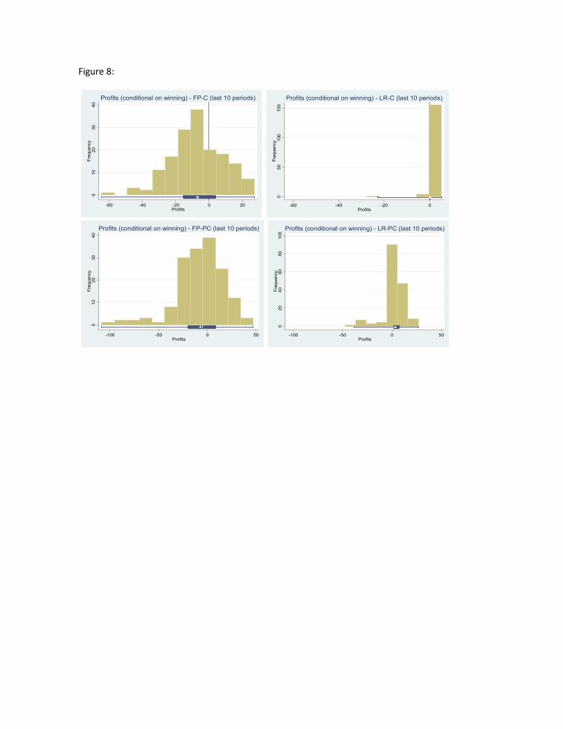
Figure 8:

010

20

30

40

Frequency

-60 -40 -20 0 20Profits

Profits (conditional on winning) - FP-C (last 10 periods)

050

100

150

Frequency

-60 -40 -20 0Profits

Profits (conditional on winning) - LR-C (last 10 periods)0

10

20

30

40

Frequency

-100 -50 0 50Profits

Profits (conditional on winning) - FP-PC (last 10 periods)

020

40

60

80

100

Frequency

-100 -50 0 50Profits

Profits (conditional on winning) - LR-PC (last 10 periods)

Figure 9:

0.1

.2.3

.4.5

Proportion


Proportion of Bids above Expected Break-Even Threshold

Winner's Curse

Figure 10:

0.2

.4.6

Proportion


1-10 11-20 1-10 11-20 1-10 11-20 1-10 11-20

Proportion of Bids above Expected Break-Even Threshold

Winner's Curse

Figure 11:

050

100

150

200

100 120 140 160 180 200Type (CV Signal)

periods 1-10 periods 11-20 Nash

E(profit)<0 Profit<0 |s Profit<0

Bidding in FP-C

Figure 12:

050

100

150

200

100 120 140 160 180 200CV Signal

periods 1-10 periods 11-20

Nash Profit<0

Bidding in LR-C

Figure 13:

050

100

150

200

-20 0 20 40 60Type (surplus)

periods 1-10 periods 11-20 Nash

E(profit)<0 Profit<0 |s

Bidding in FP-PC

Figure 14:

050

100

150

200

Bids

01020304050Type (Private Cost)

periods 1-10 periods 11-20

Nash Profit<0

Bidding in LR-PC