Socioeconomic Status and Learning from Financial

Information∗

Camelia M. Kuhnen† Andrei C. Miu‡

November 2015

Abstract

The majority of lower socioeconomic status (SES) households do not have anystock investments, which is detrimental to wealth accumulation. Here, we examineone potential driver of this puzzling fact, namely, that SES may influence the processby which people learn from information in financial markets. We find that low SESindividuals, relative to medium or high SES ones, form more pessimistic beliefs aboutthe distribution of stock investment outcomes and are less likely to invest in stocks. Thepessimism bias in assessing risky assets induced by low SES is robust to several waysof measuring one’s socioeconomic standing. These results, documented in controlledexperimental settings in Romania and the U.S., as well as in a large non-laboratorysample of adults across all 50 states in the U.S., suggest that SES shapes in predictableways people’s beliefs about financial assets, which in turn may induce large differencesacross households in their propensity to participate in financial markets.

∗We thank Stephan Siegel, Ken Singleton, seminar participants at the University of North Carolina, DukeUniversity, New York University, Yale University, and participants at the 2014 meeting of the Society forNeuroeconomics and 2015 American Economics Association meeting for helpful comments and discussion.Andreea Beciu, Claire Murray, Luke Murray and Ryan Trocinsky provided excellent research assistance. Allremaining errors are ours.

†University of North Carolina, Kenan-Flagler Business School, Finance Area, 300 Kenan Center Drive,MC #4407, Chapel Hill, NC 27599, USA. E-mail: camelia kuhnen@kenan-flagler.unc.edu. (Correspondingauthor)

‡Babes-Bolyai University, Department of Psychology, Republicii St. #37, Cluj-Napoca 400015, Romania.E-mail: andreimiu@psychology.ro.

I. Introduction

A puzzling pattern in household finance is that more than 50% of people in the U.S. and

Europe do not invest in the stock market (Campbell (2006), Calvet et al. (2007)). The

avoidance of equity investments is particularly prevalent among those less well-off. Among

households in the bottom quintile of the income distribution in the U.S., 89% have no stock

holdings, while among those in the upper quintile, more than 82% have such holdings.1 From

a policy perspective, it is important to understand the drivers of these substantial differences

in the investment choices of households across the socioeconomic spectrum.

Here we investigate a potential driver of these differences, which so far has received little

attention in the literature, namely, that the beliefs held by people regarding the distribution

of returns in equity markets may be shaped by these individuals’ socioeconomic status.

Specifically, we ask whether people’s socioeconomic status change the way they learn from

financial information and make investment decisions.

Recent evidence suggests that encountering economic adversity has a significant influence

on how people make economic choices, in particular by changing the way they learn from

new information and form beliefs about future outcomes. Chronic poverty and bad economic

shocks have been shown to be detrimental to cognitive performance (Hackman and Farah

(2009), Mani et al. (2013)). Early-life adversity in particular has long-lasting effects on

brain development and function, for example by changing the brain’s response to stress or

by diminishing memory function (Evans and Schamberg (2009)). Poverty causes stress and

negative affective states (Haushofer and Fehr (2014)), which may lead to suboptimal choices

such as underinvestment in education, undersaving, or overborrowing (Banerjee and Duflo

(2007), Shah et al. (2012)).

Aside from impeding decision-making in general, economic adversity is likely to also in-

duce a pessimism bias in how people view the distribution of future outcomes they can attain.

1Survey of Consumer Finances Chartbook, p. 507-510, issued by the Federal Reserve Board in September2014, available at http://www.federalreserve.gov/econresdata/scf/files/BulletinCharts.pdf.

1

Specifically, neuroscience research has found that individuals who have experienced adversity

exhibit a stronger brain response to negative outcomes, relative to positive outcomes. That

is, those coming from more adverse environments display increased threat vigilence as well

as a weaker response to rewarding outcomes (e.g., Nusslock and Miller (2015) and Hanson

et al. (2015)).

Therefore, the natural hypothesis that stems from these insights from neuroscience is

that individuals coming from environments with more economic adversity, who are thus

characterized by a lower socieoconomic status (SES), have more pessimistic beliefs about

the outcomes of financial investment opportunities, and that these pessimistic beliefs arise

from the fact that these lower SES individuals, unlike the rest of the population, will react

less to good news relative to bad news about such investments. In other words, our cur-

rent understanding about the effects of adversity on brain function suggests that economic

adversity induces an asymmetry in how people learn from financial or economic news, such

that those coming from lower SES environments will have a more pessimistic assessment of

available economic or financial opportunities.

There is some indirect evidence from recent work in finance and economics that aligns

with this prediction. Specifically, individuals who live through bad economic times subse-

quently avoid risky investments (Malmendier and Nagel (2011)), and those who experience

sequences of negative financial outcomes form overly pessimistic beliefs about the future re-

turns of risky assets (Kuhnen (2015)). Survey data indicates that people with less education

have more pessimistic expectations about macroeconomic growth (Souleles (2004)).

In this paper, we use a controlled experimental setting to examine whether indeed people’s

socioeconomic background changes the way they learn from new financial information and

make investment decisions. As hypothesized based on insights from neuroscience research, we

find that low SES participants, relative to medium or high SES ones, form more pessimistic

beliefs about the distribution of outcomes of risky financial assets (stocks) and are less likely

to invest in these assets. The pessimism bias regarding stocks that is induced by coming from

2

a low SES environment is particularly strong in situations when, objectively, these assets

are likely to have high payoffs, and when participants are actively investing, rather than

passively learning, and financial losses are possible. Given our experimental design, we can

isolate the role of SES on beliefs and investing decisions from confounding factors such as

SES-based differences in opportunities to invest or in financial knowledge. We replicate these

experimental findings in samples from two countries – Romania and the U.S. – and then test

the external validity of our experimental results by collecting SES, beliefs and investment

decisions data from a large non-laboratory sample of adults from all 50 states in the U.S.

Across all these three populations, encompassing more than 1400 people, we consistently

find that low SES individuals are more pessimistic about the distribution of stock returns

and are less likely to invest in stocks.

As the first step in our study, we sough to investigate in a controlled experimental setting

whether learning from new information depends on people’s socioeconomic background. To

do so, we invited participants from a top public university in Romania to a financial decision

making study, for which we used the same experimental design as in Kuhnen (2015). We ran

the experiment at that university because there we can observe a large amount of variation in

the socioeconomic status of the participant population, and, at the same time, a high degree

of homogeneity in terms of scholastic achievement. Two institutional details lead to these

features of our experimental setting: first, the students at this university are admitted based

on their performance on a stringent, national-level exam; second, the Romanian government

provides scholarships to all students who need financial assistance for covering the cost of

attending this university, and 67% of those enrolled receive such aid.

We then checked whether the results from the original laboratory sample replicate in

a different experimental pool of subjects, and conducted the experiment at a top public

university in the U.S., where we verified that the findings from the original setting replicate

out of sample, across the two countries.

Lastly, we sought to test the external validity of our laboratory results and collected data

3

regarding beliefs about stock market returns, and investment decisions from a large sample

of U.S. adults across all 50 states. As expected based on the results of the laboratory exper-

iments, we found that adults from low SES backgrounds – namely those with lower income,

lower education, faced with significant recent negative financial shocks, or living in coun-

ties with lower incomes, lower education or more unemployment – have a more pessimistic

assessment of future stock market returns and invest a lower share of their income in stocks.

The controlled experiment done by our laboratory subjects required participants to com-

plete two financial decision making tasks. In the Active task subjects made sixty decisions,

split into ten separate blocks of six trials each, to invest in one of two securities: a stock with

risky payoffs coming from one of two distributions (good and bad), one which was better

than the other in the sense of first-order stochastic dominance, and a bond with a known

payoff. In each trial, participants observed the dividend paid by the stock, after making their

asset choice, and then were asked to provide an estimate of the probability that the stock

was paying from the good distribution. Therefore, the stock dividend history seen by each

participant does not depend on whether or not they chose the stock. In other words, the

asset choice did not change the learning problem faced by participants. In the Passive task

subjects were only asked to provide the probability estimate that the stock was paying from

the good distribution, after observing its payoff in each of sixty trials, which were also split

into ten separate learning blocks of six trials each. In either task, two types of conditions -

gain or loss - were possible. In the gain condition, the two securities provided positive pay-

offs only. In the loss condition, the two securities provided negative payoffs only. Subjects

were paid based on their investment payoffs and the accuracy of the probability estimates

provided.

Importantly, the learning problem faced by subjects was exactly the same, irrespective

of their socioeconomic status. Hence, people’s estimate regarding the probability that the

stock was paying from the good dividend distribution, namely that distribution where the

high outcome for that condition was more likely to occur than the low outcome, should not

4

depend on whether a participant has encountered more or less economic adversity in life.

However, we find that low SES participants form subjective estimates for the likelihood

that the stock is paying from the good distribution that are 2.86% lower than those of mid or

high SES participants, in situations where objectively the stock is likely to be the good one.

If subjects are actively investing and they are in loss condition trials, this wedge in beliefs

becomes 4.70%. These results are robust to multiple approaches through which the low, mid

and high SES groups are constructed, and replicate out of the original Romanian sample,

in a group of U.S. participants. This pessimism bias induced by low SES is not driven by

differences in risk preferences or finance-relevant knowledge, but rather, by differences in

updating from new information. In particular, we find that when high stock dividends are

revealed, low SES participants update their beliefs less, by 3% to 5%, relative to mid or high

SES participants. That is, lower SES participants are less likely to pay attention to good

news about the available financial assets. We also show that while participants on average

improve over time their ability to correctly estimate the probability that the stock is paying

from the good distribution, the rate of improvement is slower for the low SES group relative

to the others. Finally, we document that, relative to mid and high SES people, low SES

individuals not only have a more pessimistic assessment of the stock outcome distribution,

but they also are less likely to invest in the stock. We find that in cases when the stock is

the optimal investment choice given the dividends observed so far, low SES participants are

5% less likely to choose the stock compared to their mid and high SES peers.

We checked whether our laboratory results have external validity by employing an outside

company (Qualtrics) to recruit on our behalf a sample of approximately 1200 adults ages

18 to 65 across the U.S. and who were representative of the general population in terms

of their income distribution. These adults resided in 591 different counties, across all 50

U.S. states. In line with the findings of our controlled experiments, in this non-laboratory

sample we find that individuals from lower SES backgrounds are more pessimistic about the

stock market and invest a lower share of their income in stocks. For example, we find that

5

people whose household income is in the lowest tercile in the sample (i.e, under $35,000)

on average estimate the probability that the U.S. stock market will have a positive return

over the following year to be 47.70%, whereas the same subjective estimate is 58.69% for

people whose household income is in the highest tercile (i.e., $75,000 or higher). At the

same time, we find that the share of income invested in stocks is on average 7.94% for

people in the lowest income tertile and 21.59% for people in the top income tertile. College

educated participants assess on average the probability that the U.S. stock market would

have a positive return over the following year to be 55.46%, whereas the estimate provided

by people without a college degree is 48.73%. Moreover, college educated participants invest

on average 19.07% of their income in stocks, whereas people without a college degree invest

on average only 9.24% of their income in stocks. Also, individuals who, as of early 2015, have

not encountered financial difficulties since 2007 assess the probability that U.S. stock market

will have a positive return over the next year to be 53.05%, whereas the estimate of those

who have encountered financial difficulties since 2007 is 49.65%. Those participants without

financial difficulties invest on average 16.79% of their income in stocks, whereas those who

have encountered financial trouble invest only 9.07% of their income in stocks. When instead

of participants’ self-reported own income, education or indicators of negative financial shocks

we use objective U.S. Census county-level data regarding median household income, college

education rates or unemployment rates, we continue to find the expected results: namely,

people residing in counties with worse economic conditions are more pessimistic about the

returns of the U.S. stock market, and invest a lower share of their income in stocks.

The results in this paper could help shed light on the empirical pattern documented by

Campbell (2006) and Calvet et al. (2007), namely, that U.S. and European households with

lower education, income or wealth are less likely to participate in the stock market. A poten-

tial driver of this pattern could be that lower SES households have more pessimistic beliefs

about the possible outcomes of risky investments, as observed in our study. Thus, overly

pessimistic beliefs about risky asset returns may help explain why lower SES households are

6

less likely to invest in equities.

Our findings contribute to the recent experimental finance literature on learning in mar-

kets and to the household finance literature on stock market participation. Payzan-LeNestour

and Bossaerts (forthcoming) show that people can learn about financial assets according to

Bayes’ rule, if changes in the outcome distributions of risky assets are made salient. If that is

not the case, learning performance deteriorates significantly. Beshears et al. (2013) find that

investors are unable to learn well from processes that mean-revert slowly. Investors’ learning

process depends, incorrectly, on their prior investment choices (Kuhnen et al. (2015)) and

prior choices suboptimally influence future trading decisions (Frydman and Camerer (2015)).

Beshears et al. (2015) find that low income individuals reduce their investment rates upon

learning about the contributions to retirement accounts of their work peers, and suggest that

discouragement from social comparisons may drive this effect.

We describe the experimental design in Section II. In Section III we present the main

result, as well as robustness checks, tests of alternative explanations, and external validity

tests. We discuss implications of the pessimism bias induced by encountering economic

adversity for and suggest avenues for future research building on this finding in Section IV.

II. Experimental design

For the controlled laboratory experiment we recruited 203 participants in the study (53

males, 150 females, mean age 21.3 years, 2 years standard deviation) via on-campus flyers

at the Babes-Bolyai University, which is a top higher-education institution in Romania.

Participants gave written informed consent, as required by human subjects protection rules.

All payments to participants for their performance in the experiment were provided in RON ,

which is the local currency. (1 RON is approximately equal to 0.3 USD.)

Following the same experimental protocol as in Kuhnen (2015), each participant com-

pleted two financial decision making tasks, referred to as the Active task and the Passive

7

task, during which information about two securities, a stock and a bond, was presented.

Whether a participant was presented with the Active task first, or the Passive task first,

was determined at random. Each task included two types of conditions: gain or loss. In

the gain condition, the two securities provided positive payoffs only. The stock payoffs were

+10 RON or +2 RON , while the bond payoff was +6 RON . In the loss condition, the two

securities provided negative payoffs only. The stock payoffs were -10 RON or -2 RON , while

the bond payoff was -6 RON . The task included gain and loss blocks, in both the active

and passive version, as learning may differ across these settings (Kuhnen (2015)).

In either the gain or the loss condition, the stock paid dividends from either a good

distribution or from a bad distribution. The good distribution is that where the high outcome

occurs with 70% probability in each trial, while the low outcome occurs with 30% probability.

The bad distribution is that where these probabilities are reversed: the high outcome occurs

with 30% probability, and the low outcome occurs with 70% probability in each trial.

Each participant went through 60 trials in the Active task, and 60 trials in the Passive

task. Trials are split into ”learning blocks” of six: for these six trials, the learning problem

is the same. That is, the computer either pays dividends from the good stock distribution

in each of these six trials, or it pays from the bad distribution in each of the six trials.

At the beginning of each learning block, the computer randomly selects (with 50%-50%

probabilities) whether the dividend distribution to be used in the following six trials will be

the good or the bad one.

There are ten learning blocks in the Active task, and ten learning blocks in the Passive

task. In either task, there are five blocks in the gain condition, and five blocks in the loss

condition. The order of the blocks is randomized. An example of a sequence of loss or gain

learning blocks the a subject may face during either the Active task or the Passive task, as

well as a summary of the experimental design, are shown in Table I.

In the Active task participants made 60 decisions (six per each of the ten learning blocks)

to invest in one of the two securities, the stock or the bond, then observed the stock payoff

8

(irrespective of their choice) and provided an estimate of the probability that the stock was

paying from the good distribution. Figure 1 shows the time line of a typical trial in the Active

task, in either the gain and or the loss conditions (top and bottom panel, respectively).

In the Passive task participants were only asked to provide the probability estimate that

the stock was paying from the good distribution, after observing its payoff in each of 60 trials

(split into ten learning blocks of six trials each, as in the Active task). Figure 2 shows the

time line of a typical trial in the Passive task, in either the gain or the loss conditions.

In the Active task participants were paid based on their investment payoffs and the

accuracy of the probability estimates provided. Specifically, they received one tenth of

accumulated dividends, plus ten cents for each probability estimate within 5% of the objective

Bayesian value. In the Passive task, participants were paid based solely on the accuracy of

the probability estimates provided, by receiving ten cents for each estimate within 5% of the

correct value. Information regarding the accuracy of each subject’s probability estimates and

the corresponding payment was only provided at the end of each of the two tasks. This was

done to avoid feedback effects that could have changed the participants’ strategy or answers

during the progression of each of the two tasks.

This information was presented to participants at the beginning of the experiment, and is

summarized in the participant instructions sheet included in the Appendix. The experiment

lasted 1.5 hours and the average payment per person was 28.69 RON .

The value of the objective Bayesian posterior that the stock is paying from the good

distribution can be easily calculated. Specifically, after observing t high outcomes in n trials

so far, the Bayesian posterior that the stock is the good one is: 11+ 1−p

p∗( q

1−q)n−2t

, where p = 50%

is the prior that the stock is the good one (before any dividends are observed in that learning

block) and q = 70% is the probability that a good stock pays the high (rather than the low)

dividend in each trial. The Appendix provides the value of the objective Bayesian posterior

for all {n, t} pairs possible in the experiment. This Bayesian posterior is our benchmark for

measuring how close the subjects’ expressed probability estimates are from the objectively

9

correct beliefs.

For each participant we also obtained measures of their financial literacy and risk aversion.

We obtained these two measures by asking subjects two questions regarding a portfolio

allocation problem, after they completed the Active and Passive investment tasks. These

questions are described in the Appendix. Briefly, the first question asked how much of a

10,000 RON portfolio the participant would allocate to the stock market and how much to

a savings account. This answer provides a proxy for their risk preference, measured outside

of the financial learning experiment. The second question asked the person to calculate

the expected value of the portfolio they selected, and through multiple-choice answers could

detect whether people lacked an understanding of probabilities, of the difference between net

and gross returns, or of the difference between stocks and savings accounts. This yielded a

financial knowledge score of 0 to 3, depending on whether the participant’s answer showed

an understanding of none, one, two or all three of these concepts.

Participants also completed an 11-item numeracy questionnaire as in Peters et al. (2006),

which measured their ability to do simple algebraic calculations and use information about

probabilities.

Our main measure of socioeconomic status for this sample of young adults is obtained

as in Ensminger et al. (2000) by aggregating information we obtain from each participant

regarding their parents’ income and education, their family size, and closeness of family ties.

We split the overall group of 203 participants into a low SES subsample (67 individuals),

and a mid or high SES subsample (136 individuals), based on whether their aggregate SES

score is in the low third or the upper two thirds of the SES scores distribution. As a second

way to measure of SES, we split the sample depending on whether the parental income is

below or above 1000 RON/month (approximately $300), which is the minimum full-time

wage in Romania. As a third way to measure of SES, we split the sample based on whether

the participants’ subjective assessment of whether they rank in society on a scale from 1 to

10 is below 5. Finally, as a fourth way to measure of SES, we split the sample in based on

10

whether neither of the participants’ parents have a college degree.

III. Results

A. Main result

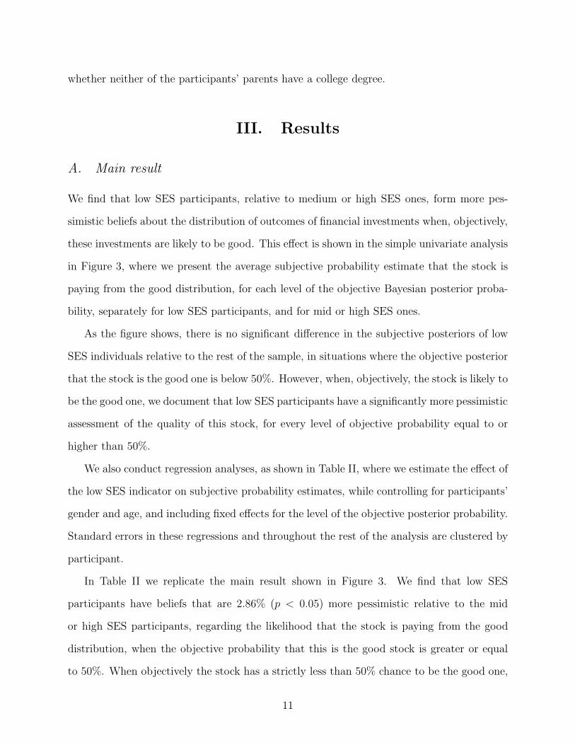
We find that low SES participants, relative to medium or high SES ones, form more pes-

simistic beliefs about the distribution of outcomes of financial investments when, objectively,

these investments are likely to be good. This effect is shown in the simple univariate analysis

in Figure 3, where we present the average subjective probability estimate that the stock is

paying from the good distribution, for each level of the objective Bayesian posterior proba-

bility, separately for low SES participants, and for mid or high SES ones.

As the figure shows, there is no significant difference in the subjective posteriors of low

SES individuals relative to the rest of the sample, in situations where the objective posterior

that the stock is the good one is below 50%. However, when, objectively, the stock is likely to

be the good one, we document that low SES participants have a significantly more pessimistic

assessment of the quality of this stock, for every level of objective probability equal to or

higher than 50%.

We also conduct regression analyses, as shown in Table II, where we estimate the effect of

the low SES indicator on subjective probability estimates, while controlling for participants’

gender and age, and including fixed effects for the level of the objective posterior probability.

Standard errors in these regressions and throughout the rest of the analysis are clustered by

participant.

In Table II we replicate the main result shown in Figure 3. We find that low SES

participants have beliefs that are 2.86% (p < 0.05) more pessimistic relative to the mid

or high SES participants, regarding the likelihood that the stock is paying from the good

distribution, when the objective probability that this is the good stock is greater or equal

to 50%. When objectively the stock has a strictly less than 50% chance to be the good one,

11

there is no SES difference in subjective probabilities. We can reject (p < 0.05) the hypothesis

that the effect of low SES on the subjective estimate of the probability that the stock is the

good one is the same for situations when objectively this probability is strictly below 50%

(first column in Table II) as when it is equal to or higher than 50% (second column in Table

II).2

Moreover, the regressions in the leftmost four columns in Table II show that the pessimism

bias regarding risky investments that is induced by coming from a low SES environment is

particularly strong if participants are actively investing, rather than passively learning, and if

financial losses are possible. In these types of trials (i.e., in the Active task, in loss condition

blocks), the beliefs expressed by low SES participants are on average 4.70% (p < 0.05) more

pessimistic than those of mid or high SES participants. Unsurprisingly, in light of the prior

literature on gender effects on investing (e.g., Barber and Odean (2001)), we also find that

men have more optimistic assessments of the quality of the stock, relative to women, in most

of the sample splits done in the analysis in Table II.

To check whether these findings are robust to our measure of low SES, in Table III we

conduct the same type of regression analyses as in Table II using the other three ways to

measure SES discussed in Section II. For ease of comparison, we present the coefficient

estimates for our main low SES measure (obtained in Table II) in Panel A of Table III.

We then assign participants to low socioeconomic status based on parental income (Panel

B), subjective socioeconomic status evaluation (Panel C), or parental education (Panel D).

The low SES measures in Panels A, B and C have similar effects: lower SES participants,

categorized this way using either of these three approaches, have more pessimistic beliefs

regarding the quality of the stock. However, if SES is assessed solely based on whether or

2In unreported models similar to the regression in the second column in Table II, we show that low SEShas a significant and negative effect on the subjective probability that the stock is paying from the gooddistribution separately in situations when the objective probability is strictly below 50%, as well as when itis exactly equal to 50%. The estimated effects of low SES on the subjective probability in these two subsetsof trials are -2.65% (p < 0.1) and -3.6% (p < 0.05), respectively. Hence we group these two subsets of trialstogether (i.e., these are the trials when the objective probability that the stock is the good one is equal orgreater than 50%) in the main analysis.

12

not neither parent of a participant got a college education, we no longer observe a significant

pessimism bias in the low SES participants (i.e., those whose parents do not have college

degrees). This suggests a possibility that needs investigation in further work, namely, that

pessimism in assessing financial investments may be triggered by aspects of SES related to

low income or financial difficulties, and not necessarily by a lack of formal higher education

of one’s parents.

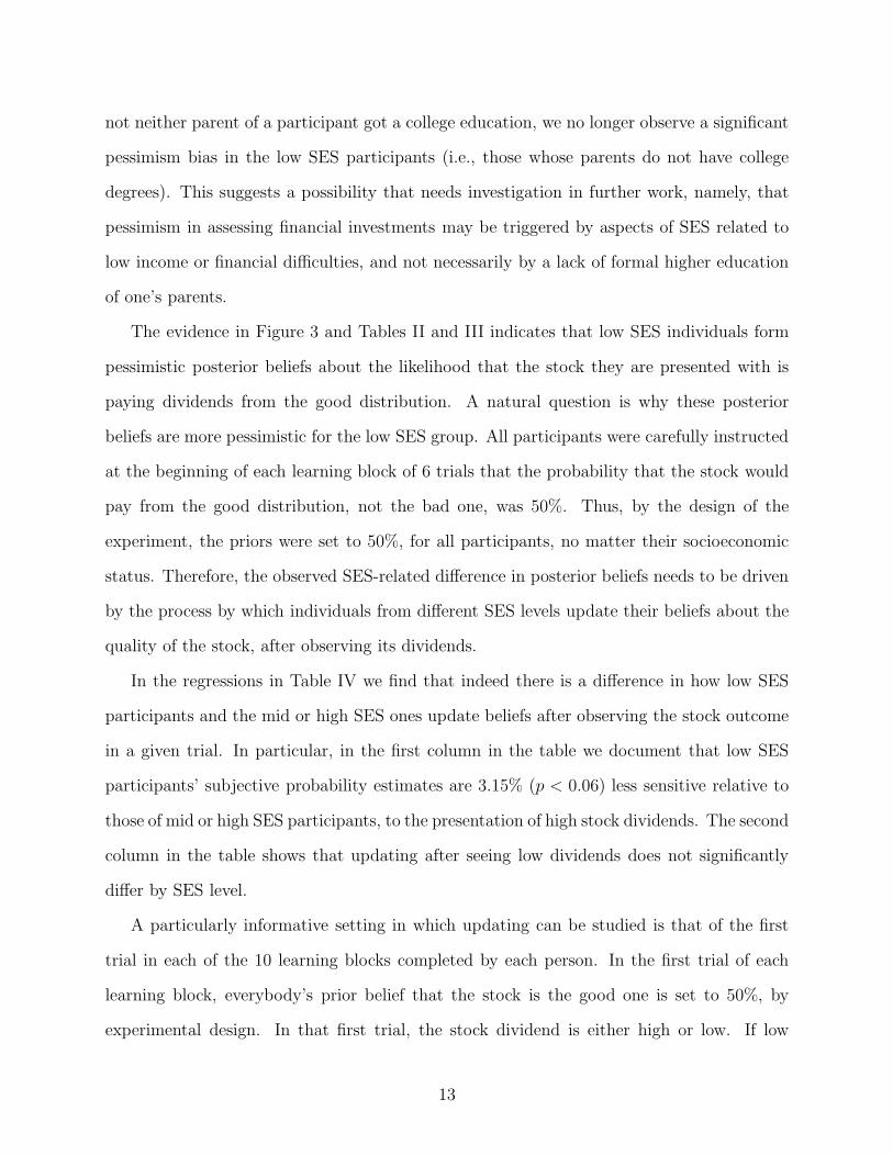
The evidence in Figure 3 and Tables II and III indicates that low SES individuals form

pessimistic posterior beliefs about the likelihood that the stock they are presented with is

paying dividends from the good distribution. A natural question is why these posterior

beliefs are more pessimistic for the low SES group. All participants were carefully instructed

at the beginning of each learning block of 6 trials that the probability that the stock would

pay from the good distribution, not the bad one, was 50%. Thus, by the design of the

experiment, the priors were set to 50%, for all participants, no matter their socioeconomic

status. Therefore, the observed SES-related difference in posterior beliefs needs to be driven

by the process by which individuals from different SES levels update their beliefs about the

quality of the stock, after observing its dividends.

In the regressions in Table IV we find that indeed there is a difference in how low SES

participants and the mid or high SES ones update beliefs after observing the stock outcome

in a given trial. In particular, in the first column in the table we document that low SES

participants’ subjective probability estimates are 3.15% (p < 0.06) less sensitive relative to

those of mid or high SES participants, to the presentation of high stock dividends. The second

column in the table shows that updating after seeing low dividends does not significantly

differ by SES level.

A particularly informative setting in which updating can be studied is that of the first

trial in each of the 10 learning blocks completed by each person. In the first trial of each

learning block, everybody’s prior belief that the stock is the good one is set to 50%, by

experimental design. In that first trial, the stock dividend is either high or low. If low

13

SES participants update less from high dividends, we should observe that their subjective

probability estimates after that first dividend in the learning block is revealed to be high

will be lower than the estimates produced by mid or high SES participants who observe the

same high dividend. The results in the third column of Table IV present evidence consistent

with this prediction: after seing a high dividend in the first trial of a new learning block, low

SES participants produce subjective probability estimates that are 4.53% (p < 0.08) lower

than those of their mid or high SES counterparts. The last column in the table shows that

when the first dividend in a new learning block is low, there is no significant difference in

the posterior beliefs of participants, depending on their SES level.

Therefore, the evidence in Table IV suggests that asymmetric updating is the likely

mechanism through which low SES participants become pessimistic regarding the quality

of the financial assets available to them: they do not update as much as the higher SES

participants from news that would indicate that these assets are in fact of good quality. That

is, low SES participants may have a skewed view of the financial investments surrounding

them: more of a view akin to “the glass is half-empty” rather than “the glass is half-full”,

consistent with neuroscience evidence that adverse environments predispose the brain to

react relatively more to bad outcomes relative to good outcomes (e.g., Nusslock and Miller

(2015)).

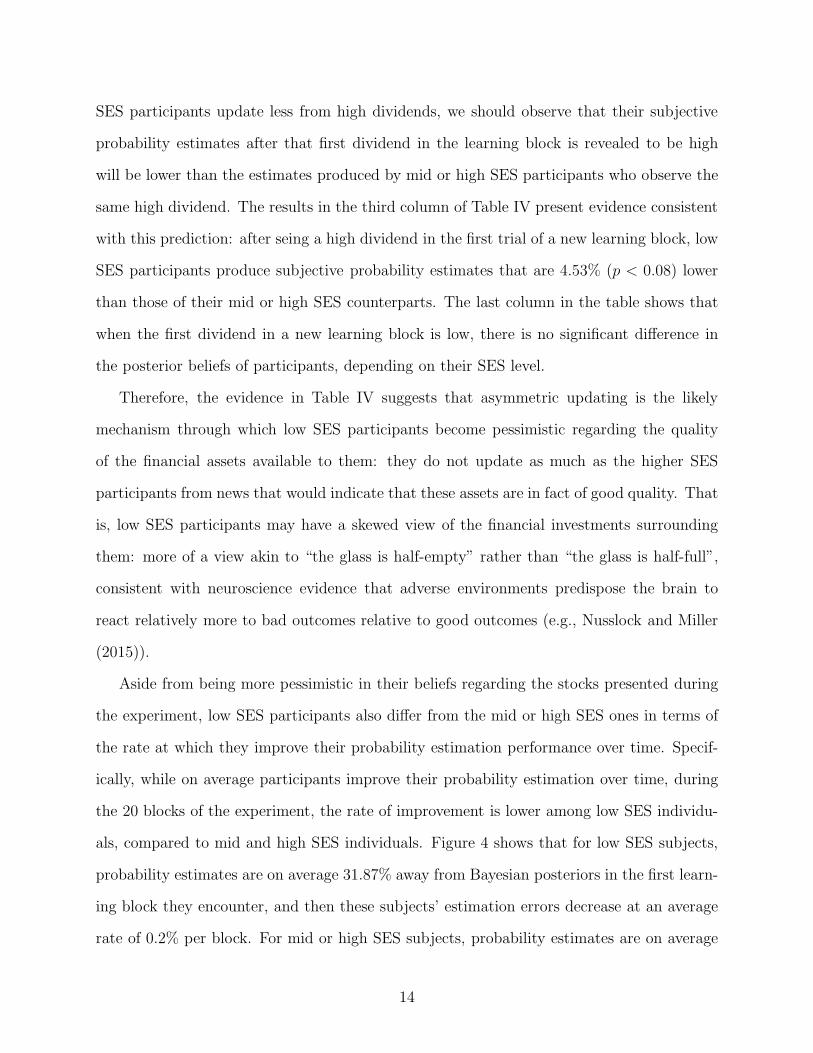
Aside from being more pessimistic in their beliefs regarding the stocks presented during

the experiment, low SES participants also differ from the mid or high SES ones in terms of

the rate at which they improve their probability estimation performance over time. Specif-

ically, while on average participants improve their probability estimation over time, during

the 20 blocks of the experiment, the rate of improvement is lower among low SES individu-

als, compared to mid and high SES individuals. Figure 4 shows that for low SES subjects,

probability estimates are on average 31.87% away from Bayesian posteriors in the first learn-

ing block they encounter, and then these subjects’ estimation errors decrease at an average

rate of 0.2% per block. For mid or high SES subjects, probability estimates are on average

14

31.18% away from Bayesian posteriors in the first learning block they encounter, and then

their estimation errors decrease at an average rate of 0.35% per block. The rate of improve-

ment in probability estimation for low SES participants is significantly lower than that for

mid or high SES participants (p < 0.05).

B. Replication study in a different experimental sample

To examine whether the results obtained in the original sample of participants replicate in

other populations, we recruited 33 participants from the University of North Carolina at

Chapel Hill. These U.S.-based individuals completed the Active version of the experiment

only, as the original Romanian sample results indicated no SES effects in the Passive version.

The Active task was identical to that used in the Romanian sample, except for having the

stock and bond payoffs expressed in U.S. dollars, instead of RON. As done in the original

sample, in the replication sample we assign participants to the low SES category if they have

SES scores which are in the bottom third of the distribution.

We find that in the U.S. sample, people from a low SES background form more pessimistic

estimates of the probability that they are faced with the good stock, relative to those from

middle or high SES backgrounds. This result, which replicates the main finding from the

Romanian sample documented in Table II, is shown in Table V. As in the original sample,

in the replication sample we find that the effect of low SES on subjective beliefs about the

stock is particularly large when objectively, the stock is likely to be the good one, and during

loss condition trials, when participants face negative outcomes.

Thus, across two samples in two different countries, we document that coming from more

economically disadvantaged backgrounds predicts that people will have a more pessimistic

assessment regarding the outcomes of financial investments available to them in our experi-

mental setting.

15

C. Alternative explanations

C.1. Do risk aversion and finance knowledge differ across SES categories?

While the evidence so far suggests that low SES participants form opinions about the quality

of investment opportunities differently from mid or high SES participants, it is possible

that there are other SES-related factors, unrelated to updating, that would lead to these

differences in subjective probability estimates in the low SES versus the mid or high SES

group. For example, it could be that low SES participants are not more pessimistic in

how they update their view about investments, but they have lower levels or finance-related

knowledge that would allow them to do well in this learning task. We find that this is not the

case in our sample. We use four measures of finance-relevant knowledge: the subjects’ scores

on the financial knowledge questions detailed in Section II, their numeracy score calculated

as in Peters et al. (2006), the type of college major they pursued (technical or not), and the

average confidence they reported when expressing their probability estimate every trial.

Table VI presents averages of these four variables related to the subjects understanding

of finance-relevant concepts, separately for the low SES subsample, and the mid or high SES

subsample. We find that neither one of these four dimensions of finance-relevant knowledge

differs significantly across the two subsamples, as shown by the p-values in the last column

in the table.

Another potential explanation for our main effect is that perhaps low SES participants

are more risk averse than the mid or high SES participants, and their subjective probability

estimates reflect their increased risk aversion, and not pessimism in their true beliefs. We

analyze four measures of risk aversion to see whether they are different for the low SES group

relative to the rest of participants.

First, for each person we calculate the frequency with which they chose the stock, rather

than the bond, in the first trial in each learning block. In this trial the choice is solely

driven by risk preferences and not by new information, since no dividend of the stock has

16

yet been observed, and thus participants only know the 50% prior that the stock is the

good one. As shown in the first row of Table VII, the difference in the propensity to chose

the stock in the first trial between the low SES group and the other participants is not

significantly different from 0 at conventional levels. Second, we compare the amount (out

of a hypothetical 10,000 RON endowment) that subjects would invest in the stock market

rather than an investment account, for the low SES group and the mid or high SES group,

and again find no significant difference, as shown in the second row of the table. The third

and fourth measures of risk attitudes shown in the bottom two rows of Table VII are given

by subjects’ scores on two surveys used widely in the psychology literature, the State-Trait

Anxiety Inventory (Spielberger et al. (1983)) and the Behavioral Inhibition Scale (Carver

and White (1994)). We do not find any differences between the low SES and the mid or high

SES groups on these anxiety-related proxies for risk avoidance.

Furthermore, as a robustness check we include the personal characteristics from Tables VI

and VII, such as finance knowledge and risk aversion, as additional explanatory variables in

our main analysis in Table II and continue to find that the effect of low SES on the subjective

probability that the stock is the good one is negative and significant (full estimation results

omitted here for brevity). For example, after adding financial knowledge, numeracy, an

indicator for whether the participant pursues a technical college major, and the state and

trail anxiety measures to the regression in column 2 of Table II, the effect of low SES on the

subjective probability estimate is -3.43% (t-stat = -2.34), similar to the effect found without

these additional explanatory variables (-2.85%, t-stat=1.98).

C.2. Do low SES participants exhibit pessimism or are they in general less able

to update correctly?

If low SES participants were simply less able to update, their probability estimates would

be significantly higher than those of mid and high SES participants in situations when the

objective probability that the stock is the good one is less than 50%. However, as Figure

17

3 shows, this is not the case. That is, when the stock is unlikely to be the good one, the

estimates of both types of participants are equally far from the correct, objective probability

(the 45◦ grey line in the figure). The same conclusion can be drawn when comparing the

first two columns in Tables II, III and V. Specifically, across the original Romanian sample

and the replication sample in the US, using various measures of SES, the evidence points

to relative pessimism on behalf of low SES participants relative to mid and high SES ones

when the stock is likely to be the good one, but not to relative optimism when the stock is

unlikely to be good. Hence, we do not find evidence of a general lack of updating ability

among low SES participants, but rather, we find evidence consistent with belief errors in a

specific direction, namely, that of pessimism about the stock return distribution in situations

when objectively the stock is likely to have good outcomes.

D. Consequences for investment choices

The pessimistic assessment of the quality of the stock payoff distribution observed among

the low SES participants has consequences for these individuals’ investment choices. Specif-

ically, as shown in Figure 5, low SES individuals are significantly less likely to choose the

stock, particularly in trials when the objective probability that the stock is paying from the

good dividend distribution is greater than 50%. In such trials, risk-neutral expected value

maximizing investors would choose to hold the stock rather than the bond.

However, we find that in these situations low SES participants choose the stock, rather

than the bond, in 74% of the trials, whereas the mid and high SES participants choose the

stock in 79% of the trials (the difference is significant at p < 0.05). That is, in cases when

the stock is the optimal investment choice given the dividends observed so far, low SES

participants are less likely to choose the stock compared to their mid and high SES peers,

and thus get a smaller payoff by choosing the bond.3

3In the Romanian laboratory sample we observed that subjects sometimes chose the stock instead of thebond even in situations when the objective probability that the stock was the good one was strictly less than50%, and hence the bond would have been the optimal choice for a risk-neutral agent, as can be inferred

18

E. External validity test: Large sample evidence from the U.S.

The evidence from our laboratory experiment run in Romania and replicated in the U.S.

indicates that lower SES experiment participants are more pessimistic in their assessment

of the available stock investment and less willing to choose the stock over the bond. The

natural next step is to inquire whether these findings are also present among populations

outside of college laboratory samples, in situations when people are considering actual stocks

instead of experimental assets, and whether our findings are robust to other ways in which

a person’s SES is measured.

Since the participants in the experimental task in the laboratory were all college students

(thus young and not yet fully employed or fully educated), for these individuals we measured

their SES based on the demographic characteristics (e.g., income and education) of their

parents. It is thus important to check whether in older samples of individuals, who vary in

SES because of their own (not their parents’) income, education or other circumstances, we

still observe that lower SES people view stocks in a more pessimistic manner and are less

likely to invest in them.

To test the external validity of the findings of our experiment, we contracted with

Qualtrics, a well-known provider of on-line survey services, to recruit on our behalf approx-

imately 1200 individuals across all 50 U.S. states, across ages 18-65, and across all income

levels such as to be representative of the income distribution according to the U.S. Census.

Each of the 1207 individuals who were in the final sample provided by Qualtrics, recruited

during April-May 2015 from 591 different counties across all U.S. states, answered several

demographics questions. These questions, which are detailed in Appendix D, included ask-

ing participants about their age, gender, education, income level, zipcode of residence and

history of financial difficulties since 2007, the beginning of the recent economic turmoil.

The sample characteristics are presented in Table VIII and indicate that the individuals

from Figure 5. This tendency was reduced, yet not completely, in the U.S. laboratory sample, which mayindicate an interesting cultural difference in people’s approach to investment decisions, something which weleave for future research to examine in depth.

19

recruited by Qualtrics are indeed very diverse and representative of the U.S. population.

Household income is below $15,000 for 13.12% of participants and above $100,000 for 18.89%

of participants, with other income levels being also very well represented in the sample. In

terms of education, 41.34% of participants have a college degree. Males represent 51.20% of

the sample. Participants’ ages vary from 18 to 65, with middle-aged people being the most

represented – for example, people with ages between 30-39 years old make up 21.96% of the

sample, and those with ages 40-49 years old make up 22.45% of the sample. About 45.15% of

the sample reported having at least one of seven types of financial difficulties since 2007. The

seven types of financial difficulties we asked participants about are: bankruptcy, foreclosure

of property, loss of employment, the inability to pay debts on time, difficulty getting approved

for loans, for example to buy a car or a house, having accounts in collection, or borrowing

from a payday lender.

After the demographics-related questions, participants were asked two additional ques-

tions, to elicit their beliefs about the possible outcomes of investing in the U.S. stock market,

and their actual investment choices. These two questions were worded as in the Michigan

Survey of Consumers, which has provided an aggregate index of consumer sentiment for

many years, and are as follows: (1) “What do you think is the percent chance that a $1000

investment in a diversified stock mutual fund will increase in value in the year ahead, so that

it is worth more than $1000 one year from now?”; and (2) “Currently, what percentage of

your income do you invest in the stock market? Include investments in directly-owned stocks,

stocks in mutual funds and stocks in retirement accounts, such as 401(K)s or IRAs.”

Question (1) above reveals the subjective probability of the individual that the aggregate

U.S. stock market will have a positive return over the following year, and this quantity is

a good real-life parallel to the subjective probability estimate that the participants in the

laboratory experiment had to provide. That is, both in the sample of experimental subjects

and in the regular adult sample surveyed by Qualtrics, we obtain a measure of people’s

belief that stocks are good investments. Question (2) above measures the individual’s actual

20

investment behavior, in terms of their decision to invest in stocks, and it is the real-life

parallel of the measure we used in the laboratory experiment, which referred to people’s

decision to choose the stock instead of the bond in any given trial.

If our laboratory findings have external validity, then we should observe that in the

sample of 1207 adults surveyed by Qualtrics on our behalf, the lower SES individuals would

have a more pessimistic assessment of the probability that the U.S. stock market would have

a positive return over the subsequent year, and would invest a lower fraction of their income

in stocks. As shown in Figure 6 the data provide strong support for these predictions. In the

figure we present the participants’ answers to questions (1) and (2) above – namely, their

belief about stock investments, and the share of income they invest in stocks – for different

subsamples of individuals based on their SES level. As our measure of participants’ SES, we

use their household income in the top panel of Figure 6, education in the middle panel of

Figure 6, and whether or not since 2007 they encountered any of the seven types of financial

difficulties listed above.

No matter which SES measure we use, we find that adults with lower SES indeed have

more pessimistic beliefs about the U.S. stock market and they invest a lower percentage

of their income in stocks. For example, the data in the top panel of Figure 6 shows that

people whose household income is in the lowest tercile in the sample (i.e., under $35,000)

on average estimate the probability that the U.S. stock market will have a positive return

over the following year to be 47.70%, whereas the same subjective estimate is 58.69% for

people whose household income is in the highest tercile (i.e., $75,000 or higher). These

probability estimates are significantly different at p < 0.01. People in the middle tertile

of income also report significantly lower probability estimates than those in the top tertile

(49.33% vs. 58.69%, p < 0.01). Importantly, not only do those earning less have a more

pessimistic assessment of the U.S. stock market, but they also invest a lower share of their

income in stocks. Specifically, we find that the average share of income invested in stocks is

7.94% for people in the lowest income tertile, 11.89% for people in the middle income tertile,

21

and 21.59% for people in the top income tertile. The differences between the income share

invested in stocks of individuals in the top income tertile and those in the lowest two income

tertiles are significant at p < 0.01.

The same pattern emerges when we measure SES by education, or by the presence of

financial difficulties in the recent recession since 2007. The middle panel of Figure 6 shows

that college educated participants assess on average the probability that the U.S. stock

market would have a positive return over the following year to be 55.46%, whereas the

estimate provided by people without a college degree is 48.73% (the difference is significant

at p < 0.01). Moreover, college educated participants invest on average 19.07% of their

income in stocks, whereas people without a college degree invest on average only 9.24% of

their income in stocks (the difference is significant at p < 0.0). The data in the bottom panel

of Figure 6 shows that individuals who have not encountered financial difficulties since 2007

assess on average the probability that U.S. stock market will have a positive return over

the next year to be 53.05%, whereas the estimate of those who have encountered financial

difficulties since 2007 is 49.65% (the p-value of the difference is 0.08). Those participants

without financial difficulties invest on average 16.79% of their income in stocks, whereas

those who have encountered financial trouble invest only 9.07% of their income in stocks

(the difference is significant at p < 0.01).

This evidence strongly indicates that the survey participants with lower SES are more

pessimistic about the stock market and less inclined to invest in stocks, thus supporting the

findings from our experimental laboratory setting. However, there exists the concern that

perhaps those individuals we surveyed were not truthful about their income, education or

financial troubles and biased their answers in such as way that we ended up observing those

reporting lower SES also reporting more pessimistic beliefs about stocks and a reluctance to

invest in stocks. While we have no reason to believe that misreporting happened, and that

it happened in this very specific manner that would drive all the results in Figure 6, it is

important to investigate if our results disappear once we have objective measures of these

22

individuals’ SES. Luckily, we can do this, as in the survey we asked participants (before they

saw any questions about their income, financial troubles or the stock market) to tell us the

five-digit zipcode in which they reside.4 We then identified the county to which each zipcode

belongs. 5 This allows us to obtain county-level data from the American Community Survey

conducted by U.S. Census regarding each county’s demographics and economic conditions.

The data are from the 2013 release (the latest available at the time this paper is written)

and provide county-level measurements of income, education or unemployment as 5-year

averages over the 2009-2013 window (one-year estimates are also available but only for the

very largest of counties in the US). These objective county-level measures can therefore

provide us with instruments for our survey participants’ income, education and economic

adversity in general, and thus will alleviate the concern that the self-reported SES measures

we get from these individuals are biased or mismeasured in general.

With these objective, county-level SES measurements in hand, in the analysis presented

in Figure 7 we conduct the same type of comparisons as in Figure 6, but instead of the

participants’ self-reported SES measures we use the county-level measures from the U.S.

Census. The results in the two figures are very similar. Even when instrumenting the

participants’ SES with county-level SES indicators, we continue to find that people in worse

economic situations, namely, people living in counties with lower income, lower education

or higher unemployment, have a more pessimistic assessment about the U.S. stock market

return over the following year and invest less of their income in stocks. For example, the

top panel of Figure 7 shows that participants in the bottom tercile in terms of county-level

household income assess the probability that the U.S. stock market will have a positive return

in the next year to be 48.91%, whereas those in the top tercile assess that probability to be

54.24% (the difference is significant at p < 0.05). These groups also invest differently: those

4This information can be verified using the geolocation information provided by Qualtrics based on theIP address of each survey participant.

5To map zipcodes to counties, we used the HUD USPS ZIP Code Crosswalk Files available atwww.huduser.gov. If a zipcode stretches across multiple counties, which happens rarely, we assigned tothat zipcode the county where more than 50% of the zipcode’s residents live.

23

in the bottom tercile, namely, living in counties with the low median household income,

invest 11.02% of their income in stocks, whereas those in the top tercile invest 15.86% of

their income in stocks (the difference is significant at p < 0.01). The middle panel of Figure

7 shows that people living in counties with below-median college education rates express

lower probabilities about the stock market having a positive return, relative to those living in

counties with above-median education (48.98% vs. 54.15%, difference significant at p < 0.01),

and also invest less of their income in stocks (10.74% vs. 16.03%, difference significant at

p < 0.01). The bottom panel of Figure 7 shows that county-level unemployment is also a

predictor of people’s beliefs about the stock market, as we find that among participants in

counties with above-median unemployment, the average subjective probability that the U.S.

stock market will have a positive return over the next year is 49.50%, whereas among those

in counties with below-median unemployment the average subjective probability is 53.54%

(the difference is significant at p < 0.05).

Overall, therefore, we find consistent evidence in support of the hypothesis of the paper,

which is that people from lower SES environments, or those characterized by more economic

adversity, have a more pessimistic assessment of the stock market and are more reluctant

to invest in stocks. This evidence comes from both controlled experimental settings in two

different countries, as well as from a large sample of participants from all of 50 states in the

U.S., which suggests that these results are robust, have external validity, and describe actual

households’ beliefs and investment decisions.

IV. Implications and conclusion

Building on insights from neuroscience which suggest that encountering adversity biases the

brain to respond less to positive outcomes relative to negative ones, we test the hypothesis

that individuals who have faced more economic adversity will have more pessimistic beliefs

regarding the possible returns of financial investments and will be less inclined to invest in

24

risky assets such as stocks.

In line with this hypothesis, we find that individuals with lower socioeconomic status

are more pessimistic compared to their more economically advantaged peers when assessing

the distribution of stock investment outcomes and invest less in stocks. These SES-related

differences in beliefs are robust to several ways of measuring one’s socioeconomic standing

and do not arise from differences in risk preferences or finance-relevant knowledge. Rather,

we document that SES induces an asymmetry in how people learn from new stock outcomes.

Specifically, we find that low SES participants are less likely to update their beliefs about

the quality of the distribution of stock outcomes when good news about stocks is revealed.

We replicate these results in two different controlled experimental settings in Romania and

the U.S. and then also show their external validity in a large sample of adults across all

50 U.S. states. Namely, we find that adults with lower income, lower education, who have

faced significant negative financial shocks during the recent economic downturn, or live in

counties with worse economic conditions, assess a lower probability that the aggregate U.S.

stock market will have a positive return over the following year, and invest a lower share of

their income in stocks.

It would be useful for future work to investigate the importance of this effect of SES on

beliefs about financial assets on the investment decisions of households over a long horizon

and on the evolution of wealth inequality between those facing low and high levels of economic

adversity. Furthermore, it remains to be established which aspects of economic adversity

matter more for the beliefs that households form regarding financial investments, and how

this may vary in different age groups. As Cronqvist and Siegel (2015) show that the influence

of the early-life environment on people’s savings behavior is highest among people in their

twenties, it is thus possible that among older adults, beliefs about financial asset returns

may be driven more by their own, rather than their parents’, socioeconomic status.

The findings in our study are important for understanding the low rates of stock mar-

ket participation observed among low SES households (Campbell (2006) and Calvet et al.

25

(2007)). It is possible that coming from a background characterized by high economic ad-

versity induces people to view financial matters through a pessimistic, “glass is half-empty”,

lens rather than in an unbiased manner. If so, then low SES people underestimate the returns

to investment in risky assets such as the stock market and may choose to avoid investing in

stocks, which may lead to more wealth inequality in the population. Further studies need

to examine these long-run effects of the SES influence on beliefs, and to test interventions

that can help reduce the SES-induced bias in people’s beliefs about the distribution of future

outcomes of risky investments.

26

REFERENCES

Banerjee, A. V. and Duflo, E.: 2007, The economic lives of the poor, Journal of Economic

Perspectives 21, 141–167.

Barber, B. M. and Odean, T.: 2001, Boys will be boys: Gender, overconfidence, and common

stock investment, Quarterly Journal of Economics 116(1), 261–292.

Beshears, J., Choi, J., Fuster, A., Laibson, D. and Madrian, B. C.: 2013, What goes up must

come down? Experimental evidence on intuitive forecasting, American Economic Review:

Papers and Proceedings 103(3), 570–574.

Beshears, J., Choi, J., Laibson, D., Madrian, B. C. and Milkman, K. L.: 2015, The ef-

fect of providing peer information on retirement savings decisions, Journal of Finance

70(3), 1161–1201.

Calvet, L. E., Campbell, J. Y. and Sodini, P.: 2007, Down or out: Assessing the welfare

costs of household investment mistakes, Journal of Political Economy 115(5), 707–747.

Campbell, J. Y.: 2006, Household finance, Journal of Finance 61(4), 1553–1604.

Carver, C. S. and White, T. L.: 1994, Behavioral inhibition, behavioral activation, and

affective responses to impending reward and punishment: The BIS/BAS scales, Journal

of Personality and Social Psychology 67, 319–333.

Cronqvist, H. and Siegel, S.: 2015, The origins of savings behavior, Journal of Political

Economy 123(1), 123–169.

Ensminger, M. E., Forrest, C. B., Riley, A. W., Kang, M., Green, B. F., Starfield, B. and

Ryan, S. A.: 2000, The validity of measures of socioeconomic status of adolescents, Jounal

of Adolescent Research 15(3), 392–418.

Evans, G. W. and Schamberg, M. A.: 2009, Childhood poverty, chronic stress, and adult

working memory, Proceedings of the National Academy of Sciences 106, 6545–6549.

27

Frydman, C. and Camerer, C.: 2015, Neural evidence of regret and its implications for

investor behavior, Working paper .

Hackman, D. A. and Farah, M. J.: 2009, Socioeconomic status and the developing brain,

Trends in Cognitive Sciences 13, 65–73.

Hanson, J. L., Albert, W. D., Iselin, A.-M. R., Carr, J. M., Dodge, K. A. and Hariri, A. R.:

2015, Cumulative stress in childhood is associated with blunted reward-related brain activ-

ity in adulthood, Social Cognitive and Affective Neuroscience doi:10.1093/scan/nsv124.

Haushofer, J. and Fehr, E.: 2014, On the psychology of poverty, Science 344(6186), 862–867.

Kuhnen, C. M.: 2015, Asymmetric learning from financial information, Journal of Finance

70(5), 2029–2062.

Kuhnen, C., Rudorf, S. and Weber, B.: 2015, Stock ownership and learning from financial

information, Working paper .

Malmendier, U. and Nagel, S.: 2011, Depression babies: Do macroeconomic experiences

affect risk-taking?, Quarterly Journal of Economics 126(1), 373–416.

Mani, A., Mullainathan, S., Shafir, E. and Zhao, J.: 2013, Poverty impedes cognitive func-

tion, Science 341, 976–980.

Nusslock, R. and Miller, G. E.: 2015, Early-life adversity and physical and emotional

health across the lifespan: A neuroimmune network hypothesis, Biological Psychiatry

doi:10.1016j.biopsych.2015.05.017.

Payzan-LeNestour, E. and Bossaerts, P.: forthcoming, Learning about unstable, publicly

unobservable payoffs, Review of Financial Studies .

Peters, E., Vastfjall, D., Slovic, P., Mertz, C., Mazzocco, K. and Dickert, S.: 2006, Numeracy

and decision making, Psychological Science 17(5), 407–413.

28

Shah, A. K., Mullainathan, S. and Shafir, E.: 2012, Some consequences of having too little,

Science 338, 682–685.

Souleles, N. S.: 2004, Expectations, heterogeneous forecast errors, and consumption: Micro

evidence from the Michigan Consumer Sentiment Surveys, Journal of Money, Credit, and

Banking 36(1), 39–72.

Spielberger, C. D., Gorsuch, R. L., Lushene, R., Vagg, P. R. and Jacobs, G. A.: 1983, Manual

for the State-Trait Anxiety Inventory, Consulting Psychologists Press, Palo Alto, CA.

29

APPENDIX

A. Participant Instructions (English Translation)

Welcome to our financial decision making study!

In this study you will work on two investment tasks. In one task you will repeatedly invest in

one of two securities: a risky security (i.e., a stock with risky payoffs) and a riskless security (i.e.,

a bond with a known payoff), and will provide estimates as to how good an investment the risky

security is. In the other task you are only asked to provide estimates as to how good an investment

the risky security is, after observing its payoffs.

In either task, there are two types of conditions you can face: the GAIN and the LOSS condi-

tions. In the GAIN condition, the two securities will only provide POSITIVE payoffs. In the LOSS

condition, the two securities will only provide NEGATIVE payoffs.

Details for the Investment Choice and Investment Evaluation Task:

Specific details for the GAIN condition:

In the GAIN condition, on any trial, if you choose to invest in the bond, you get a payoff of

6 RON for sure at the end of the trial. If you choose to invest in the stock, you will receive a

dividend which can be either 10 RON or 2 RON .

The stock can either be good or bad, and this will determine the likelihood of its dividend being

high or low. If the stock is good then the probability of receiving the 10 RON dividend is 70%

and the probability of receiving the 2 RON dividend is 30%. The dividends paid by this stock are

independent from trial to trial, but come from this exact distribution. In other words, once it is de-

termined by the computer that the stock is good, then on each trial the odds of the dividend being

10 RON are 70%, and the odds of it being 2 RON are 30%. If the stock is bad then the probability

of receiving the 10 RON dividend is 30% and the probability of receiving the 2 RON dividend is

70%. The dividends paid by this stock are independent from trial to trial, but come from this exact

distribution. In other words, once it is determined by the computer that the stock is bad, then on

each trial the odds of the dividend being 10 RON are 30%, and the odds of it being 2 RON are 70%.

Specific details for the LOSS condition:

30

In the LOSS condition, on any trial, if you choose to invest in the bond, you get a payoff of

-6 RON for sure at the end of the trial. If you choose to invest in the stock, you will receive a

dividend which can be either -10 RON or -2 RON .

The stock can either be good or bad, and this will determine the likelihood of its dividend being

high or low. If the stock is good then the probability of receiving the -10 RON dividend is 30%

and the probability of receiving the -2 RON dividend is 70%. The dividends paid by this stock

are independent from trial to trial, but come from this exact distribution. In other words, once it

is determined by the computer that the stock is good, then on each trial the odds of the dividend

being -10 RON are 30%, and the odds of it being -2 RON are 70%. If the stock is bad then the

probability of receiving the -10 RON dividend is 70% and the probability of receiving the -2 RON

dividend is 30%. The dividends paid by this stock are independent from trial to trial, but come

from this exact distribution. In other words, once it is determined by the computer that the stock

is bad, then on each trial the odds of the dividend being -10 RON are 70%, and the odds of it

being -2 RON are 30%.

In both GAIN and LOSS conditions:

In each condition, at the beginning of each block of 6 trials, you do not know which type of

stock the computer selected for that block. You may be facing the good stock, or the bad stock,

with equal probability.

On each trial in the block you will decide whether you want to invest in the stock for that trial

and accumulate the dividend paid by the stock, or invest in the riskless security and add the known

payoff to your task earnings.

You will then see the dividend paid by the stock, no matter if you chose the stock or the bond.

After that we will ask you to tell us two things: (1) what you think is the probability that the

stock is the good one (the answer must be a number between 0 and 100 - do not add the % sign,

just type in the value); (2) how much you trust your ability to come up with the correct probability

estimate that the stock is good. In other words, we want to know how confident you are that the

probability you estimated is correct. (The answer is between 1 and 9, with 1 meaning you have

the lowest amount of confidence in your estimate, and 9 meaning you have the highest level of

31

confidence in your ability to come up with the right probability estimate.)

There is always an objective, correct, probability that the stock is good, which depends on the

history of dividends paid by the stock already. For instance, at the beginning of each block of trials,

the probability that the stock is good is exactly 50%, and there is no doubt about this value.

As you observe the dividends paid by the stock you will update your belief whether or not the

stock is good. It may be that after a series of good dividends, you think the probability of the

stock being good is 75%. However, how much you trust your ability to calculate this probability

could vary. Sometimes you may not be too confident in the probability estimate you calculated

and some times you may be highly confident in this estimate. For instance, at the very beginning

of each block, the probability of the stock being good is 50% and you should be highly confident in

this number because you are told that the computer just picked at random the type of stock you

will see in the block, and nothing else has happened since then.

Every time you provide us with a probability estimate that is within 5% of the correct value

(e.g. correct probability is 80% and you say 84% , or 75%) we will add 10 cents to your payment

for taking part in this study.

Throughout the task you will be told how much you have accumulated through dividends paid

by the stock or bond you chose up to that point.

Details for the Investment Evaluation Task:

This task is exactly as the task described above, except for the fact that you will not be making

any investment choices. You will observe the dividends paid by the stock in either the GAIN or the

LOSS conditions, and you will be asked to provide us with your probability estimate that the stock

is good, and your confidence in this estimate. In this task, therefore, your payment only depends

on the accuracy of your probability estimates.

You final pay for completing the investment tasks will be:

27 RON + 1/10 * Investment Payoffs + 1/10 * Number of accurate probability estimates,

where Investment Payoffs = Dividends of securities you chose in the experiment, in both the GAIN

and the LOSS conditions.

32

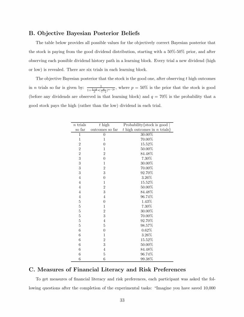
B. Objective Bayesian Posterior Beliefs

The table below provides all possible values for the objectively correct Bayesian posterior that

the stock is paying from the good dividend distribution, starting with a 50%-50% prior, and after

observing each possible dividend history path in a learning block. Every trial a new dividend (high

or low) is revealed. There are six trials in each learning block.

The objective Bayesian posterior that the stock is the good one, after observing t high outcomes

in n trials so far is given by: 11+ 1−p

p∗( q

1−q)n−2t

, where p = 50% is the prior that the stock is good

(before any dividends are observed in that learning block) and q = 70% is the probability that a

good stock pays the high (rather than the low) dividend in each trial.

n trials t high Probability{stock is good |so far outcomes so far t high outcomes in n trials}1 0 30.00%1 1 70.00%2 0 15.52%2 1 50.00%2 2 84.48%3 0 7.30%3 1 30.00%3 2 70.00%3 3 92.70%4 0 3.26%4 1 15.52%4 2 50.00%4 3 84.48%4 4 96.74%5 0 1.43%5 1 7.30%5 2 30.00%5 3 70.00%5 4 92.70%5 5 98.57%6 0 0.62%6 1 3.26%6 2 15.52%6 3 50.00%6 4 84.48%6 5 96.74%6 6 99.38%

C. Measures of Financial Literacy and Risk Preferences

To get measures of financial literacy and risk preferences, each participant was asked the fol-

lowing questions after the completion of the experimental tasks: “Imagine you have saved 10,000

33

RON . You can now invest this money over the next year using two investment options: a stock

index mutual fund which tracks the performance of the stock market, and a savings account. The

annual return per dollar invested in the stock index fund will be either +40% or -20%, with equal

probability. In other words, it is equally likely that for each RON you invest in the stock market,

at the end of the one year investment period, you will have either gained 40 cents, or lost 20 cents.

For the savings account, the known and certain rate of return for a one year investment is 5%. In

other words, for each RON you put in the savings account today, for sure you will gain 5 cents at

the end of the one year investment period. We assume that whatever amount you do not invest

in stocks will be invested in the savings account and will earn the risk free rate of return. Given

this information, how much of the 10,000 RON will you invest in the stock index fund? Choose an

answer that you would be comfortable with if this was a real-life investment decision. The answer

should be a number between 0 and 10,000 RON .”

After each participant wrote their answer to this question, they were asked the following: ”Let’s

say that when you answered the prior question you decided to invest x RON out of the 10,000

RON amount in the stock index fund, and therefore you put (10, 000 − x) RON in the savings

account. Recall that over the next year the rate of return on the stock index fund will be +40%

or -20%, with equal probability. For the savings account, the rate of return is 5% for sure. What

is the amount of money you expect to have at the end of this one year investment period? Please

choose one of the answers below. If you choose the correct answer, you will get a 5 RON bonus

added to your pay for this experiment. [A]. 0.5 (0.4 x - 0.2 x) + 0.05 (10,000 - x); [B]. 1.4 x + 0.8

x + 1.05 (10,000 - x); [C]. 0.4 (10,000 - x) - 0.2 (10,000 - x) + 0.05 x; [D]. 0.5 [ 0.4 (10,000 - x) - 0.2

(10,000 - x)] + 0.05 x; [E]. 0.4 x - 0.2 x + 0.05 (10,000 - x); [F]. 0.5 (1.4 x + 0.8 x) + 1.05 (10,000

- x); [G]. 1.4 (10,000 - x) + 0.8 (10,000 - x) + 1.05 x; [H]. 0.5 [ 1.4 (10,000 - x) + 0.8 (10,000 - x)]

+ 1.05 x.”

The correct answer to this question is [F]. The actual choices (if other than [F]) made by par-

ticipants indicate three different types of errors that can occur when calculating the expected value

of their portfolio holdings: the lack of understanding of statements regarding probabilities (an-

swers [B], [C], [E], [G]); the lack of understanding of the difference between net and gross returns

(answers [A],[C], [D] and [E]); and confusing the stock versus risk-free asset investments (answers

34

[C], [D], [G] and [H]). Therefore, a financial knowledge score varying between zero and three can

be constructed, based on the number of different types of errors contained in the answer provided

by each participant (i.e., zero errors for answer [F], one error for answers [A], [B] and [H], two

errors for answers [D], [E] and [G], and three for answer [C]). Hence a financial knowledge score of

3 indicates a perfect answer, while a score of 0 indicates that the participant’s answer included all

three possible types of errors.

D. Large Sample Survey (Qualtrics) Questions

We contracted with the outside firm Qualtrics, using their Panels service, for them to recruit

on our behalf approximately 1200 individuals ages 18-65 from across the U.S.A. and across income

levels such as to have the income distribution be representative of the population according to the

U.S. Census. These individuals were invited by Qualtrics Panels to take part in our short survey,

during April-May 2015. The survey questions were as follows:

What is your age? 18-22 years old/23-29 years old/30-39 years old/40-49 years old/50-59 years

old/60-65 years old

What is your gender? Male/Female

What is the highest level of education you have completed? some high school/GED/completed

high school/some college/technical and/or associates degree/college degree/some post-graduate

work/post-graduate degree/Other (please specify)

To which racial or ethnic group do you most identify?

African-American (non-Hispanic)/Asian/Pacific Islanders/Caucasian (non-Hispanic)/Latino or His-

panic/ Native American or American Indian/Other (please specify)

In which zipcode do you currently reside? Please enter your 5-digit zipcode:

35

Which of the following best describes your current employment status? Employed for wages/Self-

employed/Unemployed and looking for work/Unemployed and not looking for work/Stay-at-home

caregiver/Student/Military/Retired/Unable to work due to disability/Other (please specify)

Follow up question if unemployed: For how many months have you been unemployed?

If student: What is your family’s annual income? Under $15,000/$15,000-$24,999/$25,000-$34,999/$35,000-

$49,999/ $50,000-$74,999/$75,000-$99,999/$100,000 and over

If not student: What is your household’s annual income? Under $15,000 / $15,000-$24,999 /

$25,000-$34,999 / $35,000-$49,999 / $50,000-$74,999 / $75,000-$99,999/$100,000 and over

If not student: How many individuals are in your household? (including yourself)

If not student: How many of those individuals are children under the age of 18?

Since 2007, have you or your immediate family personally experienced any of the following? (Please

check all that apply): Bankruptcy/Foreclosure of property/Loss of employment/Inability to pay

your debts on time/Difficulty getting approved for loans, for example to buy a car or a house/Having

accounts in collection/Borrowing from a payday lender/None of the above

What do you think is the percent chance that a $1000 investment in a diversified stock mutual fund

will increase in value in the year ahead, so that it is worth more than $1000 one year from now?

Your answer, which is a percentage, should be a number between 0 and 100.

Currently, what percentage of your income do you invest in the stock market? Include investments

in directly-owned stocks, stocks in mutual funds and stocks in retirement accounts, such as 401(K)s

or IRAs. Your answer, which is a percentage, should be a number between 0 and 100.

36

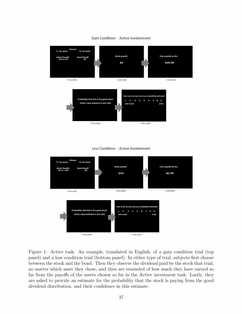
Figure 1: Active task: An example, translated in English, of a gain condition trial (toppanel) and a loss condition trial (bottom panel). In either type of trial, subjects first choosebetween the stock and the bond. Then they observe the dividend paid by the stock that trial,no matter which asset they chose, and then are reminded of how much they have earned sofar from the payoffs of the assets chosen so far in the Active investment task. Lastly, theyare asked to provide an estimate for the probability that the stock is paying from the gooddividend distribution, and their confidence in this estimate.

37

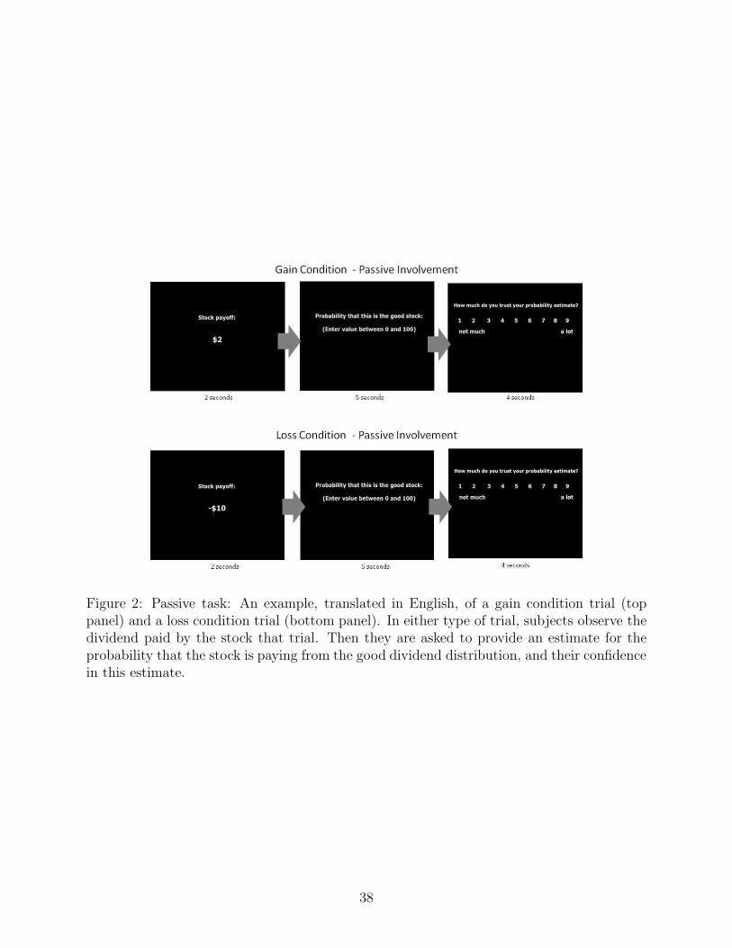
Figure 2: Passive task: An example, translated in English, of a gain condition trial (toppanel) and a loss condition trial (bottom panel). In either type of trial, subjects observe thedividend paid by the stock that trial. Then they are asked to provide an estimate for theprobability that the stock is paying from the good dividend distribution, and their confidencein this estimate.

38

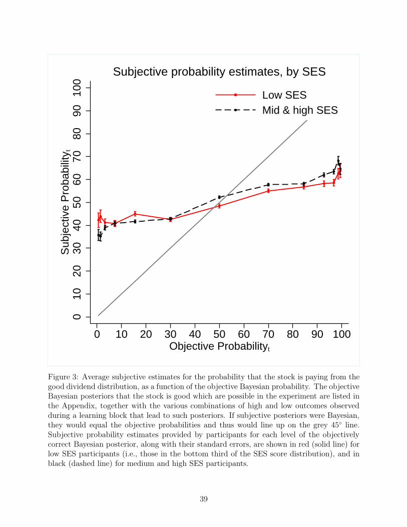
010

2030

4050

6070

8090

100

Sub

ject

ive

Pro

babi

lity t

0 10 20 30 40 50 60 70 80 90 100Objective Probabilityt

Low SESMid & high SES

Subjective probability estimates, by SES

Figure 3: Average subjective estimates for the probability that the stock is paying from thegood dividend distribution, as a function of the objective Bayesian probability. The objectiveBayesian posteriors that the stock is good which are possible in the experiment are listed inthe Appendix, together with the various combinations of high and low outcomes observedduring a learning block that lead to such posteriors. If subjective posteriors were Bayesian,they would equal the objective probabilities and thus would line up on the grey 45◦ line.Subjective probability estimates provided by participants for each level of the objectivelycorrect Bayesian posterior, along with their standard errors, are shown in red (solid line) forlow SES participants (i.e., those in the bottom third of the SES score distribution), and inblack (dashed line) for medium and high SES participants.

39

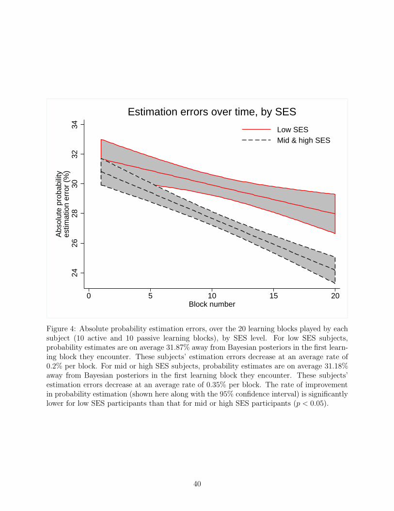
2426

2830

3234

Abs

olut

e pr

obab

ility

estim

atio

n er

ror

(%)

0 5 10 15 20Block number

Low SES Mid & high SES

Estimation errors over time, by SES

Figure 4: Absolute probability estimation errors, over the 20 learning blocks played by eachsubject (10 active and 10 passive learning blocks), by SES level. For low SES subjects,probability estimates are on average 31.87% away from Bayesian posteriors in the first learn-ing block they encounter. These subjects’ estimation errors decrease at an average rate of0.2% per block. For mid or high SES subjects, probability estimates are on average 31.18%away from Bayesian posteriors in the first learning block they encounter. These subjects’estimation errors decrease at an average rate of 0.35% per block. The rate of improvementin probability estimation (shown here along with the 95% confidence interval) is significantlylower for low SES participants than that for mid or high SES participants (p < 0.05).

40

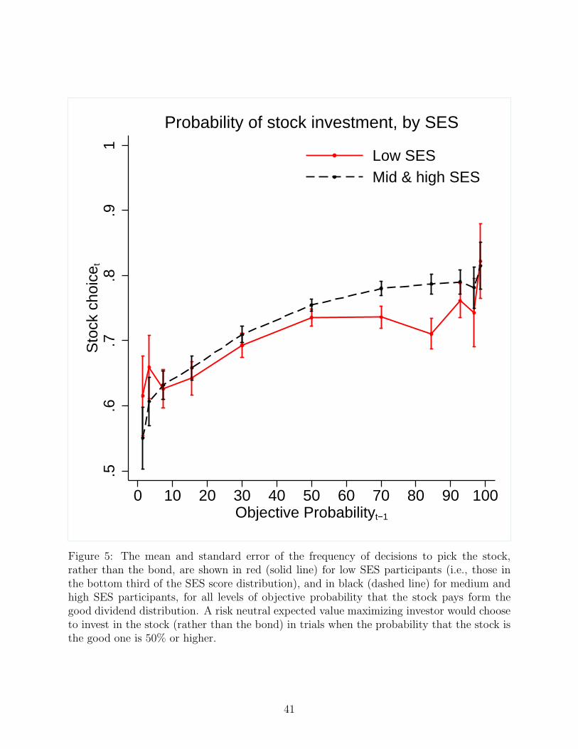
.5.6

.7.8

.91

Sto

ck c

hoic

e t

0 10 20 30 40 50 60 70 80 90 100Objective Probabilityt−1

Low SESMid & high SES

Probability of stock investment, by SES

Figure 5: The mean and standard error of the frequency of decisions to pick the stock,rather than the bond, are shown in red (solid line) for low SES participants (i.e., those inthe bottom third of the SES score distribution), and in black (dashed line) for medium andhigh SES participants, for all levels of objective probability that the stock pays form thegood dividend distribution. A risk neutral expected value maximizing investor would chooseto invest in the stock (rather than the bond) in trials when the probability that the stock isthe good one is 50% or higher.

41

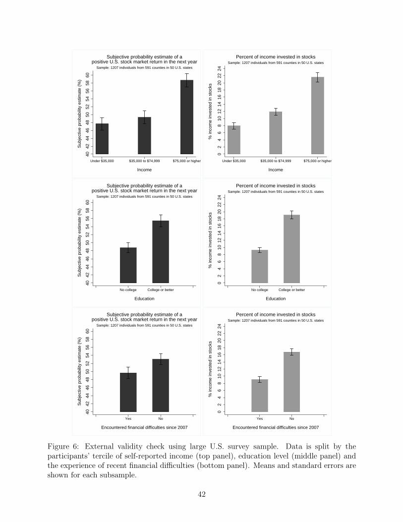
4042

4446

4850

5254

5658

60

Sub

ject

ive

prob

abili

ty e

stim

ate

(%)

Under $35,000 $35,000 to $74,999 $75,000 or higher

Income

Sample: 1207 individuals from 591 counties in 50 U.S. states

Subjective probability estimate of apositive U.S. stock market return in the next year

02

46

810

1214

1618

2022

24

% in

com

e in

vest

ed in

sto

cks

Under $35,000 $35,000 to $74,999 $75,000 or higher

Income

Sample: 1207 individuals from 591 counties in 50 U.S. states

Percent of income invested in stocks

4042

4446

4850

5254

5658

60

Sub

ject

ive

prob

abili

ty e

stim

ate

(%)

No college College or better

Education

Sample: 1207 individuals from 591 counties in 50 U.S. states

Subjective probability estimate of apositive U.S. stock market return in the next year

02

46

810

1214

1618

2022

24

% in

com

e in

vest

ed in

sto

cks

No college College or better

Education

Sample: 1207 individuals from 591 counties in 50 U.S. states

Percent of income invested in stocks

4042

4446

4850

5254

5658

60

Sub

ject

ive

prob

abili

ty e

stim

ate

(%)

Yes No

Encountered financial difficulties since 2007

Sample: 1207 individuals from 591 counties in 50 U.S. states

Subjective probability estimate of apositive U.S. stock market return in the next year

02

46

810

1214

1618

2022

24

% in

com

e in

vest

ed in

sto

cks

Yes No

Encountered financial difficulties since 2007

Sample: 1207 individuals from 591 counties in 50 U.S. states

Percent of income invested in stocks

Figure 6: External validity check using large U.S. survey sample. Data is split by theparticipants’ tercile of self-reported income (top panel), education level (middle panel) andthe experience of recent financial difficulties (bottom panel). Means and standard errors areshown for each subsample.

42

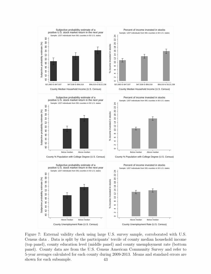
4042

4446

4850

5254

5658

60

Sub

ject

ive

prob

abili

ty e

stim

ate

(%)

$21,883 to $47,537 $47,538 to $56,018 $56,019 to $122,238

County Median Household Income (U.S. Census)

Sample: 1207 individuals from 591 counties in 50 U.S. states

Subjective probability estimate of apositive U.S. stock market return in the next year

02

46

810

1214

1618

2022

24

% in

com

e in

vest

ed in

sto

cks

$21,883 to $47,537 $47,538 to $56,018 $56,019 to $122,238

County Median Household Income (U.S. Census)

Sample: 1207 individuals from 591 counties in 50 U.S. states

Percent of income invested in stocks

4042

4446

4850

5254

5658

60

Sub

ject

ive

prob

abili

ty e

stim

ate

(%)

Below median Above median

County % Population with College Degree (U.S. Census)

Sample: 1207 individuals from 591 counties in 50 U.S. states

Subjective probability estimate of apositive U.S. stock market return in the next year

02

46

810

1214

1618

2022

24

% in

com

e in

vest

ed in

sto

cks

Below median Above median

County % Population with College Degree (U.S. Census)

Sample: 1207 individuals from 591 counties in 50 U.S. states

Percent of income invested in stocks

4042

4446

4850

5254

5658

60

Sub

ject

ive

prob

abili

ty e

stim

ate

(%)

Above median Below median

County Unemployment Rate (U.S. Census)

Sample: 1207 individuals from 591 counties in 50 U.S. states

Subjective probability estimate of apositive U.S. stock market return in the next year

02

46

810

1214

1618

2022

24

% in

com

e in

vest

ed in

sto

cks

Above median Below median

County Unemployment Rate (U.S. Census)

Sample: 1207 individuals from 591 counties in 50 U.S. states

Percent of income invested in stocks

Figure 7: External validity check using large U.S. survey sample, corroborated with U.S.Census data . Data is split by the participants’ tercile of county median household income(top panel), county education level (middle panel) and county unemployment rate (bottompanel). County data are from the U.S. Census American Community Survey and refer to5-year averages calculated for each county during 2009-2013. Means and standard errors areshown for each subsample. 43

Table I: Experimental design. Each participant goes through 60 trials in the Active task,and 60 trials in the Passive task. Whether the participant does the Active task first, orthe Passive task first, is determined at random. Trials are split into ”learning blocks” ofsix: for these six trials, the learning problem is the same. That is, the computer eitherpays dividends from the good stock distribution in each of these six trials, or it pays fromthe bad distribution in each of the six trials. The good distribution is that where the highdividend occurs with 70% probability in each trial, while the low outcome occurs with 30%probability. The bad distribution is that where these probabilities are reversed: the highoutcome occurs with 30% probability, and the low outcome occurs with 70% probability ineach trial. At the beginning of each learning block, the computer randomly selects (with50%-50% probabilities) whether the dividend distribution to be used in the following sixtrials will be the good or the bad one. There are ten learning blocks in the Active task,and ten learning blocks in the Passive task. In either task, there are five blocks in the gaincondition, and five blocks in the loss condition. The order of the blocks is randomized. Anexample of a sequence of loss or gain blocks that a participant may face is shown below.

Active Task See Figure 1 for examples of trials ConditionBlock 1 Trial 1; Trial 2; Trial 3; Trial 4; Trial 5; Trial 6 LossBlock 2 Trial 1; Trial 2; Trial 3; Trial 4; Trial 5; Trial 6 GainBlock 3 Trial 1; Trial 2; Trial 3; Trial 4; Trial 5; Trial 6 Gain

. . .

. . .

. . .Block 9 Trial 1; Trial 2; Trial 3; Trial 4; Trial 5; Trial 6 GainBlock 10 Trial 1; Trial 2; Trial 3; Trial 4; Trial 5; Trial 6 Loss

Passive Task See Figure 2 for examples of trials ConditionBlock 1 Trial 1; Trial 2; Trial 3; Trial 4; Trial 5; Trial 6 GainBlock 2 Trial 1; Trial 2; Trial 3; Trial 4; Trial 5; Trial 6 LossBlock 3 Trial 1; Trial 2; Trial 3; Trial 4; Trial 5; Trial 6 Gain

. . .

. . .

. . .Block 9 Trial 1; Trial 2; Trial 3; Trial 4; Trial 5; Trial 6 LossBlock 10 Trial 1; Trial 2; Trial 3; Trial 4; Trial 5; Trial 6 Loss

44

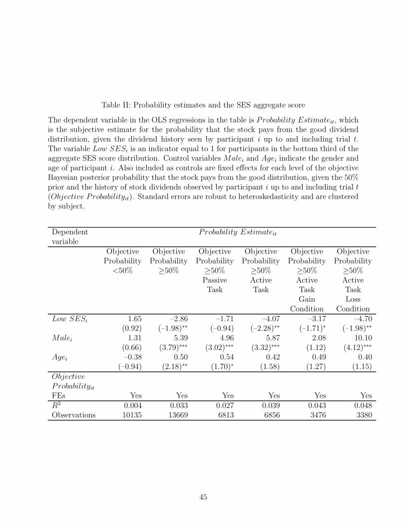
Table II: Probability estimates and the SES aggregate score

The dependent variable in the OLS regressions in the table is Probability Estimateit, whichis the subjective estimate for the probability that the stock pays from the good dividenddistribution, given the dividend history seen by participant i up to and including trial t.The variable Low SESi is an indicator equal to 1 for participants in the bottom third of theaggregate SES score distribution. Control variables Malei and Agei indicate the gender andage of participant i. Also included as controls are fixed effects for each level of the objectiveBayesian posterior probability that the stock pays from the good distribution, given the 50%prior and the history of stock dividends observed by participant i up to and including trial t(Objective Probabilityit). Standard errors are robust to heteroskedasticity and are clusteredby subject.

Dependent Probability Estimateitvariable

Objective Objective Objective Objective Objective ObjectiveProbability Probability Probability Probability Probability Probability

<50% ≥50% ≥50% ≥50% ≥50% ≥50%Passive Active Active ActiveTask Task Task Task

Gain LossCondition Condition

Low SESi 1.65 –2.86 –1.71 –4.07 –3.17 –4.70(0.92) (–1.98)∗∗ (–0.94) (–2.28)∗∗ (–1.71)∗ (–1.98)∗∗

Malei 1.31 5.39 4.96 5.87 2.08 10.10(0.66) (3.79)∗∗∗ (3.02)∗∗∗ (3.32)∗∗∗ (1.12) (4.12)∗∗∗

Agei –0.38 0.50 0.54 0.42 0.49 0.40(–0.94) (2.18)∗∗ (1.70)∗ (1.58) (1.27) (1.15)

Objective

ProbabilityitFEs Yes Yes Yes Yes Yes YesR2 0.004 0.033 0.027 0.039 0.043 0.048Observations 10135 13669 6813 6856 3476 3380

45

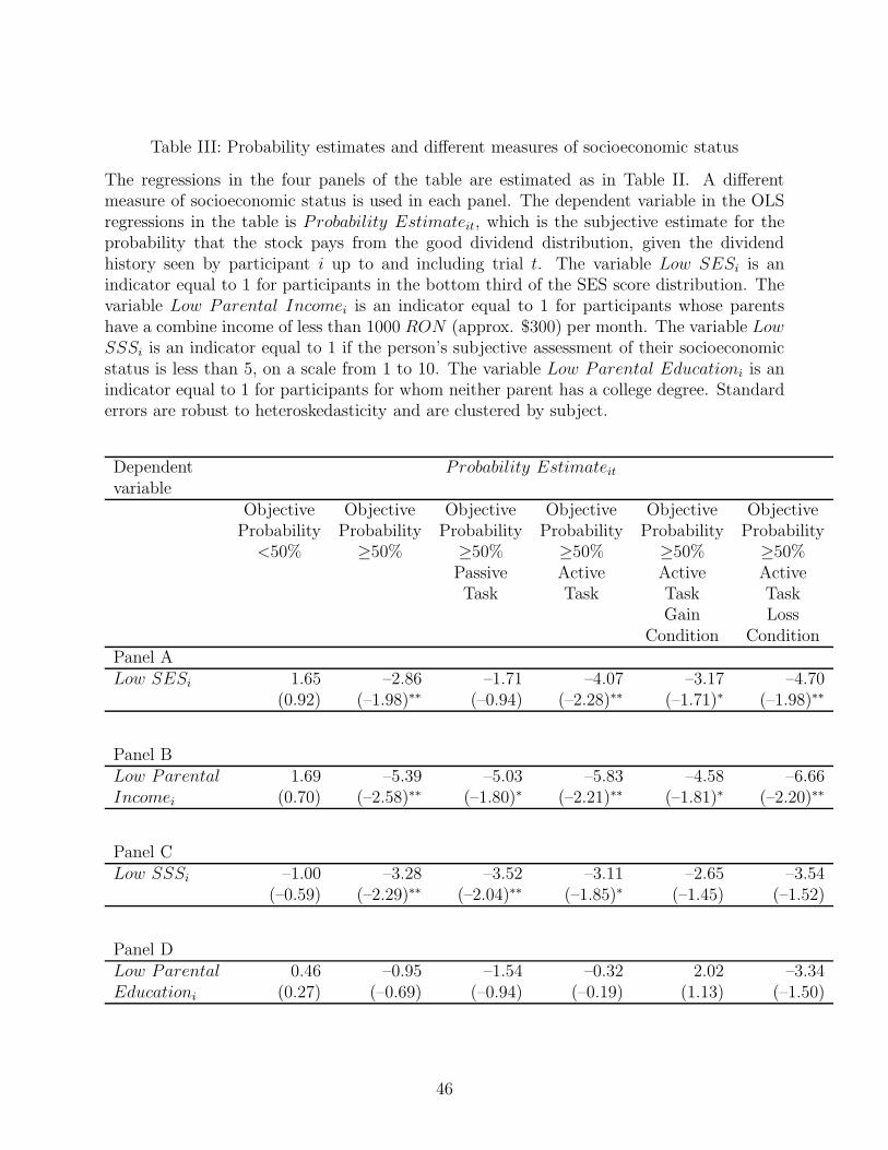
Table III: Probability estimates and different measures of socioeconomic status

The regressions in the four panels of the table are estimated as in Table II. A differentmeasure of socioeconomic status is used in each panel. The dependent variable in the OLSregressions in the table is Probability Estimateit, which is the subjective estimate for theprobability that the stock pays from the good dividend distribution, given the dividendhistory seen by participant i up to and including trial t. The variable Low SESi is anindicator equal to 1 for participants in the bottom third of the SES score distribution. Thevariable Low Parental Incomei is an indicator equal to 1 for participants whose parentshave a combine income of less than 1000 RON (approx. $300) per month. The variable LowSSSi is an indicator equal to 1 if the person’s subjective assessment of their socioeconomicstatus is less than 5, on a scale from 1 to 10. The variable Low Parental Educationi is anindicator equal to 1 for participants for whom neither parent has a college degree. Standarderrors are robust to heteroskedasticity and are clustered by subject.

Dependent Probability Estimateitvariable

Objective Objective Objective Objective Objective ObjectiveProbability Probability Probability Probability Probability Probability

<50% ≥50% ≥50% ≥50% ≥50% ≥50%Passive Active Active ActiveTask Task Task Task

Gain LossCondition Condition

Panel ALow SESi 1.65 –2.86 –1.71 –4.07 –3.17 –4.70

(0.92) (–1.98)∗∗ (–0.94) (–2.28)∗∗ (–1.71)∗ (–1.98)∗∗

Panel BLow Parental 1.69 –5.39 –5.03 –5.83 –4.58 –6.66Incomei (0.70) (–2.58)∗∗ (–1.80)∗ (–2.21)∗∗ (–1.81)∗ (–2.20)∗∗

Panel CLow SSSi –1.00 –3.28 –3.52 –3.11 –2.65 –3.54

(–0.59) (–2.29)∗∗ (–2.04)∗∗ (–1.85)∗ (–1.45) (–1.52)

Panel DLow Parental 0.46 –0.95 –1.54 –0.32 2.02 –3.34Educationi (0.27) (–0.69) (–0.94) (–0.19) (1.13) (–1.50)

46

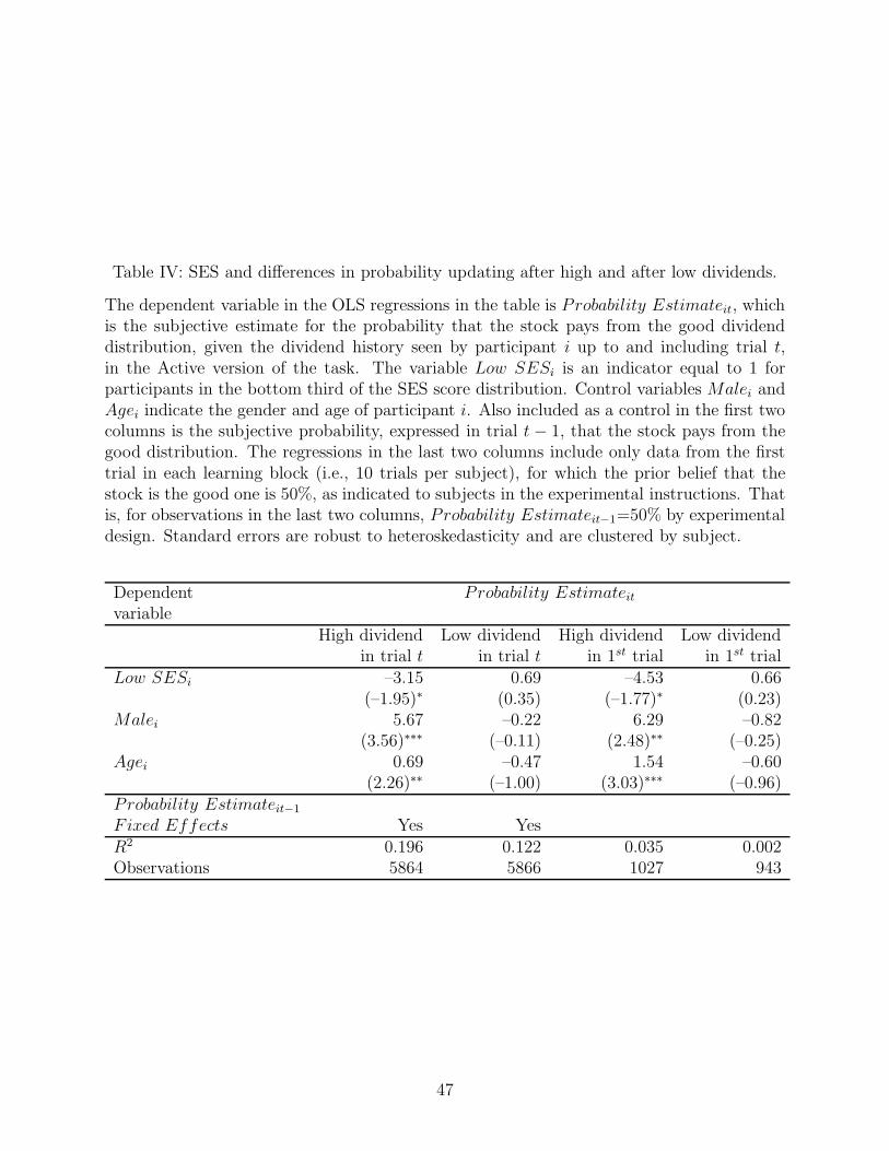
Table IV: SES and differences in probability updating after high and after low dividends.

The dependent variable in the OLS regressions in the table is Probability Estimateit, whichis the subjective estimate for the probability that the stock pays from the good dividenddistribution, given the dividend history seen by participant i up to and including trial t,in the Active version of the task. The variable Low SESi is an indicator equal to 1 forparticipants in the bottom third of the SES score distribution. Control variables Malei andAgei indicate the gender and age of participant i. Also included as a control in the first twocolumns is the subjective probability, expressed in trial t − 1, that the stock pays from thegood distribution. The regressions in the last two columns include only data from the firsttrial in each learning block (i.e., 10 trials per subject), for which the prior belief that thestock is the good one is 50%, as indicated to subjects in the experimental instructions. Thatis, for observations in the last two columns, Probability Estimateit−1=50% by experimentaldesign. Standard errors are robust to heteroskedasticity and are clustered by subject.

Dependent Probability Estimateitvariable

High dividend Low dividend High dividend Low dividendin trial t in trial t in 1st trial in 1st trial

Low SESi –3.15 0.69 –4.53 0.66(–1.95)∗ (0.35) (–1.77)∗ (0.23)

Malei 5.67 –0.22 6.29 –0.82(3.56)∗∗∗ (–0.11) (2.48)∗∗ (–0.25)

Agei 0.69 –0.47 1.54 –0.60(2.26)∗∗ (–1.00) (3.03)∗∗∗ (–0.96)

Probability Estimateit−1

Fixed Effects Yes YesR2 0.196 0.122 0.035 0.002Observations 5864 5866 1027 943

47

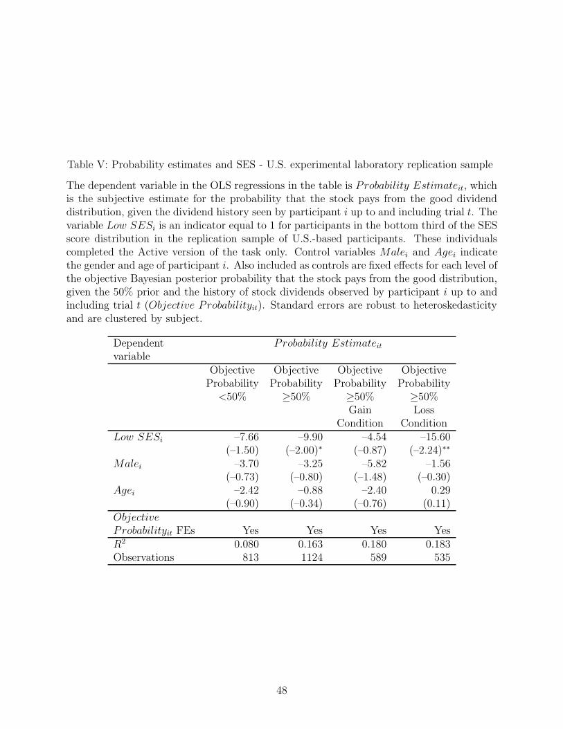
Table V: Probability estimates and SES - U.S. experimental laboratory replication sample

The dependent variable in the OLS regressions in the table is Probability Estimateit, whichis the subjective estimate for the probability that the stock pays from the good dividenddistribution, given the dividend history seen by participant i up to and including trial t. Thevariable Low SESi is an indicator equal to 1 for participants in the bottom third of the SESscore distribution in the replication sample of U.S.-based participants. These individualscompleted the Active version of the task only. Control variables Malei and Agei indicatethe gender and age of participant i. Also included as controls are fixed effects for each level ofthe objective Bayesian posterior probability that the stock pays from the good distribution,given the 50% prior and the history of stock dividends observed by participant i up to andincluding trial t (Objective Probabilityit). Standard errors are robust to heteroskedasticityand are clustered by subject.

Dependent Probability Estimateitvariable

Objective Objective Objective ObjectiveProbability Probability Probability Probability

<50% ≥50% ≥50% ≥50%Gain Loss

Condition ConditionLow SESi –7.66 –9.90 –4.54 –15.60

(–1.50) (–2.00)∗ (–0.87) (–2.24)∗∗

Malei –3.70 –3.25 –5.82 –1.56(–0.73) (–0.80) (–1.48) (–0.30)

Agei –2.42 –0.88 –2.40 0.29(–0.90) (–0.34) (–0.76) (0.11)

Objective

Probabilityit FEs Yes Yes Yes YesR2 0.080 0.163 0.180 0.183Observations 813 1124 589 535

48

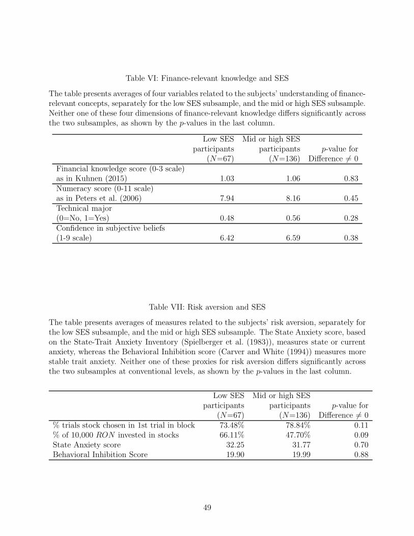
Table VI: Finance-relevant knowledge and SES

The table presents averages of four variables related to the subjects’ understanding of finance-relevant concepts, separately for the low SES subsample, and the mid or high SES subsample.Neither one of these four dimensions of finance-relevant knowledge differs significantly acrossthe two subsamples, as shown by the p-values in the last column.

Low SES Mid or high SESparticipants participants p-value for

(N=67) (N=136) Difference 6= 0Financial knowledge score (0-3 scale)as in Kuhnen (2015) 1.03 1.06 0.83Numeracy score (0-11 scale)as in Peters et al. (2006) 7.94 8.16 0.45Technical major(0=No, 1=Yes) 0.48 0.56 0.28Confidence in subjective beliefs(1-9 scale) 6.42 6.59 0.38

Table VII: Risk aversion and SES

The table presents averages of measures related to the subjects’ risk aversion, separately forthe low SES subsample, and the mid or high SES subsample. The State Anxiety score, basedon the State-Trait Anxiety Inventory (Spielberger et al. (1983)), measures state or currentanxiety, whereas the Behavioral Inhibition score (Carver and White (1994)) measures morestable trait anxiety. Neither one of these proxies for risk aversion differs significantly acrossthe two subsamples at conventional levels, as shown by the p-values in the last column.

Low SES Mid or high SESparticipants participants p-value for

(N=67) (N=136) Difference 6= 0% trials stock chosen in 1st trial in block 73.48% 78.84% 0.11% of 10,000 RON invested in stocks 66.11% 47.70% 0.09State Anxiety score 32.25 31.77 0.70Behavioral Inhibition Score 19.90 19.99 0.88

49

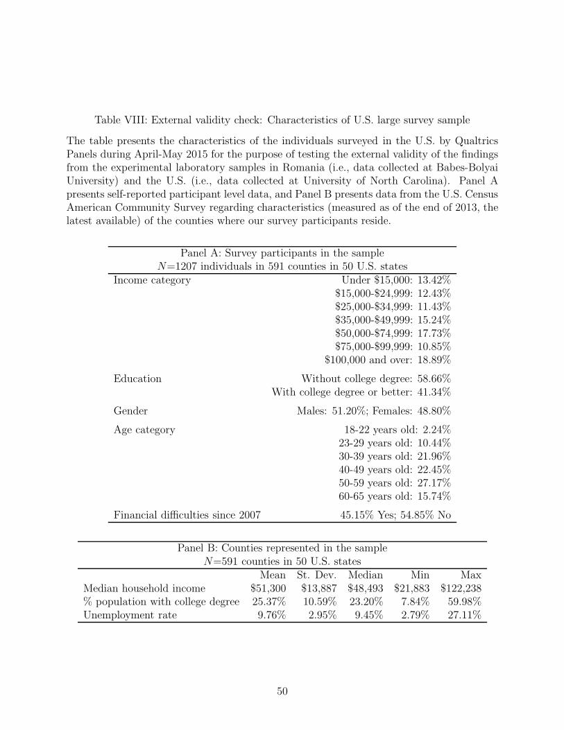
Table VIII: External validity check: Characteristics of U.S. large survey sample

The table presents the characteristics of the individuals surveyed in the U.S. by QualtricsPanels during April-May 2015 for the purpose of testing the external validity of the findingsfrom the experimental laboratory samples in Romania (i.e., data collected at Babes-BolyaiUniversity) and the U.S. (i.e., data collected at University of North Carolina). Panel Apresents self-reported participant level data, and Panel B presents data from the U.S. CensusAmerican Community Survey regarding characteristics (measured as of the end of 2013, thelatest available) of the counties where our survey participants reside.

Panel A: Survey participants in the sampleN=1207 individuals in 591 counties in 50 U.S. states

Income category Under $15,000: 13.42%$15,000-$24,999: 12.43%$25,000-$34,999: 11.43%$35,000-$49,999: 15.24%$50,000-$74,999: 17.73%$75,000-$99,999: 10.85%

$100,000 and over: 18.89%

Education Without college degree: 58.66%With college degree or better: 41.34%

Gender Males: 51.20%; Females: 48.80%

Age category 18-22 years old: 2.24%23-29 years old: 10.44%30-39 years old: 21.96%40-49 years old: 22.45%50-59 years old: 27.17%60-65 years old: 15.74%

Financial difficulties since 2007 45.15% Yes; 54.85% No

Panel B: Counties represented in the sampleN=591 counties in 50 U.S. states

Mean St. Dev. Median Min MaxMedian household income $51,300 $13,887 $48,493 $21,883 $122,238% population with college degree 25.37% 10.59% 23.20% 7.84% 59.98%Unemployment rate 9.76% 2.95% 9.45% 2.79% 27.11%

50