


Languages
Pages
Legal


The Impacts of Free Secondary Education: Evidence from Kenya
Andrew Brudevold-NewmanAmerican Institutes for Research
(AIR)
Education Evidence for Action Nyeri, Kenya
December 2017

Motivation: free education policies
Almost all countries subsidize basic education
Subsidies are designed to address:
• Positive social returns to education
• Education as a basic human right
I “Ensure that, by 2015, children everywhere, boys and girls alike, willbe able to complete a full course of primary schooling”- Millennium development goal #2 (2000)
Over a third of Sub-Saharan African countries introduced free primaryeducation policies between 1994 and 2015(Harding and Stasavage 2014, UNESCO 2015)
• These policies have been shown to increase education access andattainment, often among most vulnerable populations(Lucas & Mbiti 2012, Al-Samarrai & Zaman 2007, Hoogeveen & Rossi 2013, Deininger
2003, Grogan 2009, Nishimura et al. 2008)
Brudevold-Newman (2017) Impacts of Free Secondary Education, Slide 2

Motivation: free education policies
Countries are now expanding education systems to include freesecondary education (FSE) programs(Gambia, Kenya, South Africa, Uganda)
Might face a more muted demand response at the secondary school level:
• Opportunity cost of schooling is likely to be higher
• Returns to education may be low or perceived to be low
• Incentives of parents and children may not align
Evidence from targeted programs at the secondary school level is mixed(Gajigo 2012, Garlick 2013, Barrera-Osorio et al. 2007)
Encouraging results from a recent experiment (Duflo et al. 2017)
If FSE programs do increase educational attainment, they may alsoimpact a range of other outcomes
Brudevold-Newman (2017) Impacts of Free Secondary Education, Slide 3

Motivation: impacts on demographic outcomes
Delaying childbirth in particular could be beneficial
• Early childbearing has been associated with:
I Higher morbidity and mortality (maternal and child)
I Pregnancy related deaths are the largest cause of mortality for 15-19year old females worldwide
I Accounts for 2/3 of deaths in sub-Saharan Africa (15-19 year oldfemales) (Patton et al. The Lancet, 2016)
I Lower educational attainment
I Lower family income
(Ferre 2009 and Schultz 2008)
Mixed evidence on fertility impacts of education:
• Impacts may be conditional on high initial rates
(Osili & Long 2008, Ferre 2009, Keats 2014, Baird et al. 2010, Ozier 2016,
Filmer & Schady 2014, McCrary and Royer 2011)
Brudevold-Newman (2017) The Impacts of Free Secondary Education: Evidence from Kenya, Slide 7

Overview
Present Study: Measure the impact of FSE using the 2008introduction in Kenya
Exploit heterogeneity in ex-ante exposure to the program based on theproportion of students dropping out of school after completing primaryschool.
I measure the impact of the FSE policy on:
• Educational attainment (increased schooling by 0.8 years)
• Academic achievement (no decrease in student test scores)
I also use exposure to FSE as an instrument to measure the impact ofsecondary schooling on:
• Demographic outcomes (age of first intercourse, birth, marriage)
• Labor market outcomes (occupational choice)
(Extension) (Model)
Brudevold-Newman (2017) Impacts of Free Secondary Education, Slide 4
Context
Brudevold-Newman (2017) Impacts of Free Secondary Education, Slide 5
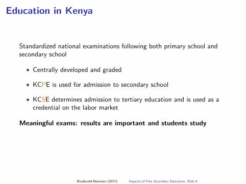
Education in Kenya
Standardized national examinations following both primary school andsecondary school
• Centrally developed and graded
• KCPE is used for admission to secondary school
• KCSE determines admission to tertiary education and is used as acredential on the labor market
Meaningful exams: results are important and students study
Brudevold-Newman (2017) Impacts of Free Secondary Education, Slide 6

FSE in Kenya
FSE introduced in January 2008
• Covered tuition at public day secondary schools
I Implemented as a capitation grant for secondary school students
I Covered KSh10,265 (∼ USD164)
I Grant equivalent to ∼22% of mean per capita householdexpenditures (Glennerster et al. 2011)
• Decreased household cost of secondary schooling
• Government also instructed schools to:
I Increase number of classes
I Increase class sizes from 40 to 45
Brudevold-Newman (2017) Impacts of Free Secondary Education, Slide 7

National trends in secondary school admission
Secondary school enrollments prior to FSE
2008 FSE0
100
200
300
400
500
600
700
Sec
. sch
ool a
dmis
sion
s (t
hous
ands
)
-6 -4 -2 0 2 4 6Year
Actual admissions
Source: Kenya Economic Surveys (2000-2013).
Brudevold-Newman (2017) Impacts of Free Secondary Education, Slide 8

National trends in secondary school admission
Secondary school enrollments prior to FSE
2008 FSE0
100
200
300
400
500
600
700
Sec
. sch
ool a
dmis
sion
s (t
hous
ands
)
-6 -4 -2 0 2 4 6Year
Actual admissions Trend line for Pre-FSE period
Source: Kenya Economic Surveys (2000-2013).
Brudevold-Newman (2017) Impacts of Free Secondary Education, Slide 9

National trends in secondary school admission
Enrollments increased following program introduction
2008 FSE0
100
200
300
400
500
600
700
Sec
. sch
ool a
dmis
sion
s (t
hous
ands
)
-6 -4 -2 0 2 4 6Year
Actual admissions Trend line for Pre-FSE period
Source: Kenya Economic Surveys (2000-2013).
Brudevold-Newman (2017) Impacts of Free Secondary Education, Slide 10

Data
Brudevold-Newman (2017) Impacts of Free Secondary Education, Slide 11

Data sources: DHS
Kenya Demographic and Health Survey (2014)
• Nationally representative survey of women aged 15-49
• Focus on individuals born between 1983 and 1996 who havecompleted primary school
I Yields a sample of 13,605 individuals (summary statistics)
• Use to calculate regional treatment intensity and estimateprogram impact on demographic and labor market outcomes
Administrative Test Scores (summary statistics)
• All students who took the KCSE between 2006 and 2015 (no 2012)
• Over 3.3 million individuals
• Exclude students from less than 1% of schools that draw fromaround the country
• Use to measure impact on academic performance
Brudevold-Newman (2017) Impacts of Free Secondary Education, Slide 12

Impacts on Educational Attainment
Brudevold-Newman (2017) Impacts of Free Secondary Education, Slide 13
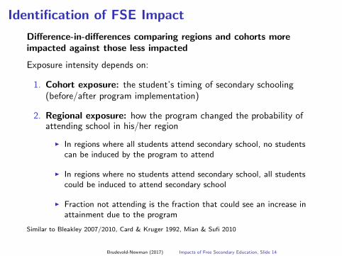
Identification of FSE Impact
Difference-in-differences comparing regions and cohorts moreimpacted against those less impacted
Exposure intensity depends on:
1. Cohort exposure: the student’s timing of secondary schooling(before/after program implementation)
2. Regional exposure: how the program changed the probability ofattending school in his/her region
I In regions where all students attend secondary school, no studentscan be induced by the program to attend
I In regions where no students attend secondary school, all studentscould be induced to attend secondary school
I Fraction not attending is the fraction that could see an increase inattainment due to the program
Similar to Bleakley 2007/2010, Card & Kruger 1992, Mian & Sufi 2010
Brudevold-Newman (2017) Impacts of Free Secondary Education, Slide 14

DHS cohort exposure implied by registration data(Return)
0.2
.4.6
.81
Den
sity
of e
xam
coh
ort
020
4060
8010
0P
erce
nt c
ohor
t tre
ated
8 10 12 14 16 18 20 22Age at time of FSE
Age distribution of primary school completion exam cohortImplied percent of cohort exposed to FSE
Source: 2014 KCPE registration data.Notes: The age distribution for the first FSE cohort (2007 primary school completers) is assumedto have been the same as that observed in the 2014 cohort. The implied cumulative distributionassumes that age distribution of test takers is stable across time.
based on the age distribution of primary school completersPercent of each cohort exposed to FSE
Comparison of 2008 cohort and 2014 cohort
Implies that students aged 16 or younger in 2007 were impactedby the program (born in 1991 or later)
Brudevold-Newman (2017) Impacts of Free Secondary Education, Slide 39

Regional exposure
02
46
810
Fre
quen
cy
.2 .4 .6 .8 1Primary to secondary transition rate
Source: 2014 Kenya DHS.Notes: Transition rate measured as students with any secondary schooling as a fraction ofprimary school graduates. Dashed line indicates mean county transition rate.
Pre-FSE county transition rates
Brudevold-Newman (2017) The Impacts of Free Secondary Education: Evidence from Kenya, Slide 32

Regional exposure trends
.4.6
.8P
rimar
y-se
cond
ary
tran
sitio
n ra
te
-6 -4 -2 0 2 4 6Cohort
High pre-program access Low pre-program accessPre-program linear trend Pre-program linear trend
Source: 2014 Kenya DHS.Notes: High/low pre-program access defined as whether county average pri-sec transition ratebetween 1989 and 1990 was above/below the average transition rate. Pri-sec transition ratedefined as share of primary school graduates with at least some secondary schooling. Freesecondary education introduced in early 2008 for the 2007 KCPE cohort. 70% of KCPE students in 2014 were 14-16 years old suggesting program first impacted students born between 1991 and 1993.
and by high/low pre-FSE program transition ratesPrimary to secondary transition rates by birth cohort
Diff-in-diff
Return
Brudevold-Newman (2017) Impacts of Free Secondary Education, Slide 16

Summary: impact of FSE on education
At the mean intensity of 0.34, estimates suggest an increase of 0.8 yearsof education.
• Smaller than primary education estimates (1-1.5 years in Nigeria andUganda)
• Larger than existing secondary school estimates (0.3 years in theGambia)
Estimates consistently suggest that FSE would induce ∼ 50% of studentsto attend and complete secondary school
• Almost equivalent estimates across genders
• No evidence for differential impacts by gender
Brudevold-Newman (2017) Impacts of Free Secondary Education, Slide 18

Impact of FSE on education
(1) (2) (3) (4) (5)
A. Pooled Gender
(1-transition rate)*FSE period 2.255∗∗∗ 2.256∗∗∗ 2.060∗∗∗ 2.059∗∗∗ 2.134∗∗∗
(0.31) (0.311) (0.356) (0.718) (0.677)Observations 13605 13605 13605 13605 13605R2 0.099 0.101 0.1 0.104 0.106
B. Female Only
(1-transition rate)*FSE period 2.409∗∗∗ 2.449∗∗∗ 2.221∗∗∗ 2.058∗∗ 2.336∗∗∗
(0.277) (0.268) (0.336) (0.897) (0.709)Observations 9596 9596 9596 9596 9596R2 0.091 0.093 0.092 0.096 0.099
C. Male Only
(1-transition rate)*FSE period 2.047∗∗∗ 2.035∗∗∗ 1.942∗∗∗ 2.374∗∗ 2.075(0.673) (0.616) (0.686) (1.090) (1.309)
Observations 4009 4009 4009 4009 4009R2 0.125 0.129 0.128 0.14 0.147
Control variables:
Constituency development funds * birth year X X2009 unemployment rate * birth year X XCounty linear trend X X
Common trends, Falsification test, No transition cohorts, No cities, No small counties
Brudevold-Newman (2017) Impacts of Free Secondary Education, Slide 17

Impacts of Secondary Education
Brudevold-Newman (2017) Impacts of Free Secondary Education, Slide 19

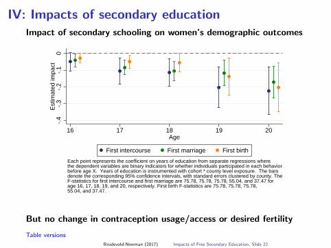
IV: Impacts of secondary educationImpact of secondary schooling on women’s demographic outcomes
-.4
-.3
-.2
-.1
0E
stim
ated
impa
ct
16 17 18 19 20Age
First intercourse First marriage First birth
Each point represents the coefficient on years of education from separate regressions wherethe dependent variables are binary indicators for whether individuals participated in each behaviorbefore age X. Years of education is instrumented with cohort * county level exposure. The barsdenote the corresponding 95% confidence intervals, with standard errors clustered by county. TheF-statistics for first intercourse and first marriage are 75.78, 75.78, 75.78, 55.04, and 37.47 forage 16, 17, 18, 19, and 20, respectively. First birth F-statistics are 75.78, 75.78, 75.78,55.04, and 37.47.
before selected agesEstimated impact of secondary education on behaviors
But no change in contraception usage/access or desired fertility
Table versions
Brudevold-Newman (2017) Impacts of Free Secondary Education, Slide 22

IV: Impacts of secondary education
Impact of secondary schooling on labor market outcomes
Skilled Unskilled Agricultural NoWork Work Work Work
(1) (2) (3) (4)
Panel 1. Age 18 and over
Years of education 0.069∗∗∗ -0.06 -0.18∗∗∗ 0.171∗∗
(0.022) (0.064) (0.039) (0.079)Observations 4525 4525 4525 4525First stage F-stat: 22.909 22.909 22.909 22.909
Panel 2. Age 19 and over
Years of education 0.074∗∗∗ -0.047 -0.169∗∗∗ 0.142∗∗
(0.023) (0.059) (0.037) (0.07)Observations 4295 4295 4295 4295First stage F-stat: 24.347 24.347 24.347 24.347
Panel 3. Age 20 and over
Years of education 0.082∗∗∗ -0.037 -0.137∗∗∗ 0.092(0.025) (0.057) (0.033) (0.067)
Observations 3935 3935 3935 3935First stage F-stat: 16.226 16.226 16.226 16.226
Brudevold-Newman (2017) Impacts of Free Secondary Education, Slide 23

Impacts of Academic Achievement
Brudevold-Newman (2017) Impacts of Free Secondary Education, Slide 24

Sample with no composition changes?
0.2
.4.6
.81
Pro
port
ion
com
plet
ing
seco
ndar
y sc
hool
0 100 200 300 400 500Primary School Completion Examination Score
2001 2010
Brudevold-Newman (2017) The Impacts of Free Secondary Education: Evidence from Kenya, Slide 51

Diff-in-diff: impacts on student achievement
Test scores in more impacted regions did not decrease
• Together with a decline in resource quality, suggests that averagestudent ability did not decline
• Suggests the presence of credit constraints
Even among the top performers for whom composition changes areunlikely, test scores did not decrease
• Suggests that lower resource quality and potentially lower abilitypeers did not decrease test scores
Brudevold-Newman (2017) Impacts of Free Secondary Education, Slide 25

Discussion & Conclusions
Brudevold-Newman (2017) Impacts of Free Secondary Education, Slide 26

Summary
Kenya introduced FSE in 2008
• The policy led to increased educational attainment of about 0.8years of schooling
• The influx of students accompanying the program did not decreasetest scores
Secondary education in Kenya has broad impacts:
• Delays age of first intercourse (∼10-25% at each teenage age)
• Delays age of first marriage (∼50% at each teenage age)
• Delays age of first birth (∼30-50% at each teenage age)
• Increases likelihood of skilled work
• Decreases probability of agricultural work
Brudevold-Newman (2017) Impacts of Free Secondary Education, Slide 27

Conclusions
Are credit constraints holding back investment in education?
• Probably. Rapid increase in attendance following FSE combined withno impact on test scores suggests presence of credit constraints.
Interpreting the demographic and labor market impacts
• Delaying behaviors not unambiguously positive.
I While there seem to be clear benefits to delaying childbirth
I Delaying age of first marriage may impact marriage market andmatch quality (Baird et al., 2016)
• Occupational choice results are encouraging
I Shifting to higher productivity sectors may promote growth(McMillan and Rodrik, 2011)
Brudevold-Newman (2017) Impacts of Free Secondary Education, Slide 28

Thank you!
Brudevold-Newman (2017) Impacts of Free Secondary Education, Slide 29

Brudevold-Newman (2017) Impacts of Free Secondary Education, Slide 30

Difference-in-differences
Compare more treated regions to less treated regions
Sijk = α0 + β1 (Ik ∗ FSEj) + Xijk + ηk + γj + εijk
• Sijk reflects the schooling of individual i in cohort j in county k
• Ik = (1− transition rate) is the intensity for county k
• FSEj is a dummy variable equal to one for individuals born incohorts impacted by FSE
• Xijk is a vector of ethnicity and religion variables
• ηk represent county fixed effects
• γj represent cohort fixed effects
The interaction coefficient, β1 is the estimate of the effect of FSEon education
Brudevold-Newman (2017) Impacts of Free Secondary Education, Slide 15

Binary difference-in-differences: primary school
(1) (2) (3) (4) (5)
A. Pooled Gender
High Intensity*FSE period -0.0005 0.00002 0.007 -0.059∗∗∗ -0.044∗(0.013) (0.013) (0.014) (0.023) (0.023)
Observations 20458 20458 20458 20458 20458
R2 0.201 0.201 0.201 0.204 0.205
B. Female Only
High Intensity*FSE period 0.006 0.005 0.014 -0.054∗ -0.032(0.015) (0.015) (0.015) (0.028) (0.028)
Observations 14934 14934 14934 14934 14934
R2 0.228 0.229 0.229 0.232 0.234
C. Male Only
High Intensity*FSE period -0.011 -0.006 -0.015 -0.057 -0.066(0.026) (0.026) (0.027) (0.038) (0.04)
Observations 5524 5524 5524 5524 5524
R2 0.153 0.155 0.155 0.164 0.17
Control variables:Constituency development funds * birth year X X2009 unemployment rate * birth year X XCounty linear trends X X
Brudevold-Newman (2017) Impacts of Free Secondary Education, Slide 31

Brudevold-Newman (2017) Impacts of Free Secondary Education, Slide 32

Primary school difference-in-differences
(1) (2) (3) (4) (5)
A. Pooled Gender
(1-transition rate)*FSE period 0.055 0.06 0.086∗∗ -0.134 -0.06(0.044) (0.044) (0.043) (0.083) (0.083)
Observations 20458 20458 20458 20458 20458
R2 0.208 0.209 0.209 0.211 0.212
B. Female Only
(1-transition rate)*FSE period 0.04 0.043 0.082 -0.129 -0.024(0.059) (0.057) (0.067) (0.098) (0.102)
Observations 14934 14934 14934 14934 14934
R2 0.228 0.229 0.229 0.232 0.234
C. Male Only
(1-transition rate)*FSE period 0.116 0.124 0.122 -0.143 -0.148(0.105) (0.107) (0.112) (0.152) (0.165)
Observations 5524 5524 5524 5524 5524
R2 0.153 0.156 0.155 0.164 0.169
Control variables:Constituency development funds * birth year X X2009 unemployment rate * birth year X XCounty linear trends X X
Note: Dependent variable is a binary variable equal to one if an individual has completed primary school. Allregressions include birth year, county, and ethnicity/religion fixed effects. Standard errors are clustered at the countylevel. Regressions are weighted using DHS survey weights. Transition rate defined as the percentage of primaryschool graduates who attend secondary school. Initial transition rate defined as the average transition rate in eachcounty for students born in either 1989 or 1990. FSE period defined as birth cohorts after and including 1991. ∗∗∗indicates significance at the 99 percent level; ∗∗ indicates significance at the 95 percent level; and ∗ indicatessignificance at the 90 percent level.
Brudevold-Newman (2017) Impacts of Free Secondary Education, Slide 33

Brudevold-Newman (2017) Impacts of Free Secondary Education, Slide 34

Kaplan-Meier survival: age of first intercourse
0.00
0.25
0.50
0.75
1.00
10 15 20 25 30Age
No secondary school Any secondary school
Return
Brudevold-Newman (2017) Impacts of Free Secondary Education, Slide 35
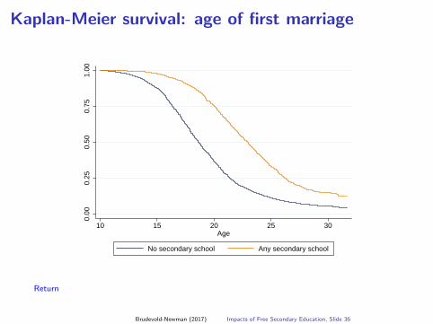
Kaplan-Meier survival: age of first marriage
0.00
0.25
0.50
0.75
1.00
10 15 20 25 30Age
No secondary school Any secondary school
Return
Brudevold-Newman (2017) Impacts of Free Secondary Education, Slide 36

Brudevold-Newman (2017) Impacts of Free Secondary Education, Slide 37

DHS cohort exposure (Return)
Official protocol calls for students to complete primary school aged13-14
• Implies first FSE cohort born in 1993 and 1994
• However, school entry age is not regularly followed and primarygrade repetition rates are high
• Older cohorts may have also been impacted
Use registration data for the KCPE to see age of birth of primaryschool completers
Brudevold-Newman (2017) Impacts of Free Secondary Education, Slide 38

DHS cohort exposure implied by registration data(Return)
0.2
.4.6
.81
Den
sity
of e
xam
coh
ort
020
4060
8010
0P
erce
nt c
ohor
t tre
ated
8 10 12 14 16 18 20 22Age at time of FSE
Age distribution of primary school completion exam cohortImplied percent of cohort exposed to FSE
Source: 2014 KCPE registration data.Notes: The age distribution for the first FSE cohort (2007 primary school completers) is assumedto have been the same as that observed in the 2014 cohort. The implied cumulative distributionassumes that age distribution of test takers is stable across time.
based on the age distribution of primary school completersPercent of each cohort exposed to FSE
Comparison of 2008 cohort and 2014 cohort
Implies that students aged 16 or younger in 2007 were impactedby the program (born in 1991 or later)
Brudevold-Newman (2017) Impacts of Free Secondary Education, Slide 39

Brudevold-Newman (2017) Impacts of Free Secondary Education, Slide 40

2008 and 2014 Cohort Age Structure (Return)
010
2030
40D
ensi
ty o
f exa
m c
ohor
t
10 12 14 16 18 20Age
2008 cohort 2014 cohort
Source: 2008 and 2014 KCPE data.Notes: 2008 data are only available for Central, Nyanza, and Western provinces. The 2014 dataare restricted to the same provinces. Data restricted to first time test takers.
for Central, Nyanza, and Western provincesAge distribution of 2008 and 2014 exam cohorts
Brudevold-Newman (2017) Impacts of Free Secondary Education, Slide 41

Brudevold-Newman (2017) Impacts of Free Secondary Education, Slide 42

Examination data cohort exposure (Return)
In full examination dataset:
• No birth cohort
• Treatment definition based on examination cohort
• Without grade repetition, first FSE cohort took KCSE in 2011
• Grade repetition is a potential threat, but is relatively low at thesecondary school level
I Matched KCPE/KCSE data indicate that 80% of students completesecondary school in 4 years
• Consider cohorts who took the KCSE in 2011 or later as treated
Histogram of time to completion
Brudevold-Newman (2017) Impacts of Free Secondary Education, Slide 43

Time between primary and secondary schoolcompletion (Return)
020
4060
80P
erce
nt
4 5 6 7 8 9Years since primary school completion
Source: 2014 KCSE Registration DataNote: Fewer than 2% of test takers complete secondary school more than 7 years after primaryschool.
Time between primary and secondary school completion
Brudevold-Newman (2017) Impacts of Free Secondary Education, Slide 44

Brudevold-Newman (2017) Impacts of Free Secondary Education, Slide 45

Administrative data: a cautionary tale (Return)
Brudevold-Newman (2017) Impacts of Free Secondary Education, Slide 46

Administrative data: a cautionary tale (Return)
Brudevold-Newman (2017) Impacts of Free Secondary Education, Slide 47

Administrative data: a cautionary tale (Return)
Brudevold-Newman (2017) Impacts of Free Secondary Education, Slide 48

Identification: impacts of secondary education (Return)
Figure suggests using:
f (Iijk) =∑6
j=1 ξ1j (Ik × γj)
where:
• Ik × γj is the interaction between the treatment intensity of county kand the cohort j
Similar to Duflo 2004
Identifying assumption is that FSE intensity only impactsdemographic or labor market variables through education
Brudevold-Newman (2017) Impacts of Free Secondary Education, Slide 49

Baseline model (Return)
• Two-period model for primary school graduatesI Period 0: individuals can either attend school or enter labor force
I Period 1: students who attended school earn wage premium
• Utility is over consumption in the two periodsI U = u (c0) + δu (c1)
• Utility from working/attending school is:I Uw = u (c0) + δu (c1) = u (1) + δu (1)
I Us (a) = u (c0) + δu (c1) = δu (h (a) − R · p)
where a is individual ability, h (a) is the premium on accumulated humancapital, p is the cost of schooling (tuition and fees), and R is a grossinterest rate
Individuals attend school if Us (a) ≥ Uw
Brudevold-Newman (2017) Impacts of Free Secondary Education, Slide 50

Model specifics (Return)
• Let a?p satisfy Us (a) = Uw
• All students with a > a?p attain greater utility from attending schoolthan from working
• Mean ability of students attending school is:
Ap =
∫ amax
a?paf (a) da∫ amax
a?pf (a) da
Eliminating tuition in this scenario lowers the price from p to pf .
• Lowers a∗ so that a∗pf < a∗p
• Induces a∗pf ≤ a < a∗p to attend school
• Lower ability students now attend secondary school
Apf =
∫ amax
a?pfaf (a) da∫ amax
a?pff (a) da
< Ap
Brudevold-Newman (2017) Impacts of Free Secondary Education, Slide 51

Model specifics with credit constraints (Return)
• A fraction of individuals, w , come from wealthy families while theremainder, 1− w , come from poor families.
• Individuals from poor families are restricted to borrowing p (a) withp′ (·) > 0
• ∀a ∈ A, p (a) < p so that the original price of schooling precludesall poor students from attending school
• Lowering the price of schooling from p → pfI Induces a∗pf ≤ a < a∗p from wealthy families to attend school
I Induces students from poor families with a > a?cc for whom the lowerprice eases the credit constraint to attend school
Ap =w ·
∫ amax
a?pfaf (a) da + (1− w) ·
∫ amax
a?ccaf (a) da
w ·∫ amax
a?pff (a) da + (1− w) ·
∫ amax
a?ccf (a) da
Increases access, ambiguous impact on average ability
Brudevold-Newman (2017) Impacts of Free Secondary Education, Slide 52

Model specifics with fertility (Return)
Utility now depends on both consumption and the quantity ofunprotected sex:
• Benefit, absent a pregnancy, of µ (s)I µ′ (·) > 0 for s < s, µ′ (·) < 0 for s ≥ s, and µ′′ (·) < 0: that is,
utility is increasing in unprotected sex to a certain level, s, abovewhich utility is decreasing in s
• Pregnancy yields a utility benefit, B > 0, and occurs with aprobability v (si )
• Individuals select a level of initial period unprotected sex, realize thepregnancy outcome, and then in the absence of a birth, select initialperiod schooling or labor
• Low ability individuals have no trade off and select a high level of sex
• High ability individuals face a trade off between sex and thepossibility of not being able to attend school
Brudevold-Newman (2017) Impacts of Free Secondary Education, Slide 53

Brudevold-Newman (2017) Impacts of Free Secondary Education, Slide 54

Binary difference-in-differences: common trends (Return)
Explicit test of common trends using pre-treatment data:
Sijk = α0 + β1 (Highk ∗ Trend) + β2Trend + Xi jk + ηk + εijk
Overall Female Male(1) (2) (3)
High*trend -0.025 -0.012 -0.067(0.034) (0.039) (0.062)
Observations 12022 8971 3051
R2 0.311 0.333 0.229
Brudevold-Newman (2017) Impacts of Free Secondary Education, Slide 55

Brudevold-Newman (2017) Impacts of Free Secondary Education, Slide 56

Binary falsification test (Return)
(1) (2) (3) (4) (5)
A. Falsification for program introduced in 1986
High Intensity*FSE period 0.198∗ 0.139 0.224∗ 0.229 0.162(0.119) (0.094) (0.126) (0.2) (0.214)
Observations 10324 10324 10324 10324 10324
R2 0.112 0.115 0.112 0.117 0.12
B. Falsification for program introduced in 1985
High Intensity*FSE period 0.184 0.126 0.222 0.152 0.121(0.13) (0.114) (0.14) (0.214) (0.204)
Observations 11142 11142 11142 11142 11142
R2 0.111 0.114 0.111 0.117 0.12
C. Falsification for program introduced in 1984
High Intensity*FSE period 0.095 0.044 0.104 -0.047 -0.157(0.104) (0.086) (0.1) (0.203) (0.21)
Observations 10643 10643 10643 10643 10643
R2 0.111 0.114 0.111 0.116 0.119
D. Falsification for program introduced in 1983
High Intensity*FSE period 0.062 0.002 0.082 -0.03 -0.06(0.116) (0.12) (0.111) (0.246) (0.231)
Observations 10264 10264 10264 10264 10264
R2 0.113 0.117 0.114 0.118 0.121
E. Falsification for program introduced in 1982
High Intensity*FSE period 0.04 0.07 0.085 0.385∗ 0.504∗∗(0.133) (0.145) (0.125) (0.207) (0.232)
Observations 9760 9760 9760 9760 9760
R2 0.113 0.115 0.114 0.118 0.121
Control variables:Constituency development funds * birth year X X2009 unemployment rate * birth year X XCounty linear trend X X
Brudevold-Newman (2017) Impacts of Free Secondary Education, Slide 57

Brudevold-Newman (2017) Impacts of Free Secondary Education, Slide 58

Difference-in-differences: no transition cohorts (Return)
(1) (2) (3) (4) (5)
Panel 1: years of education
A. Pooled Gender
High Intensity*FSE period 0.346∗∗ 0.39∗∗∗ 0.332∗∗ 0.578∗∗∗ 0.605∗∗∗
(0.146) (0.147) (0.153) (0.192) (0.186)Observations 11684 11684 11684 11684 11684R2 0.093 0.101 0.1 0.106 0.109
B. Female Only
High Intensity*FSE period 0.356∗∗ 0.416∗∗∗ 0.319∗∗ 0.725∗∗∗ 0.852∗∗∗
(0.15) (0.147) (0.155) (0.234) (0.204)Observations 8246 8246 8246 8246 8246R2 0.089 0.095 0.095 0.102 0.104
C. Male Only
High Intensity*FSE period 0.322∗ 0.389∗∗ 0.407∗ 0.274 0.151(0.194) (0.188) (0.208) (0.459) (0.473)
Observations 3438 3438 3438 3438 3438R2 0.117 0.136 0.135 0.147 0.155
Control variables:
Constituency development funds * birth year X X2009 unemployment rate * birth year X XCounty linear trend X X
Brudevold-Newman (2017) Impacts of Free Secondary Education, Slide 59

Brudevold-Newman (2017) Impacts of Free Secondary Education, Slide 60

Difference-in-differences: common trends (Return)
Explicit test of common trends using pre-treatment data:
Sijk = α0 + β1 (Ik ∗ Trend) + β2Trend + Xi jk + ηk + εijk
Overall Female Male(1) (2) (3)
High*trend 0.068 0.029 0.188(0.123) (0.139) (0.211)
Observations 12022 8971 3051R2 0.311 0.333 0.229
Brudevold-Newman (2017) Impacts of Free Secondary Education, Slide 61

Brudevold-Newman (2017) Impacts of Free Secondary Education, Slide 62

Falsification test (Return)
(1) (2) (3) (4) (5)
A. Pooled Gender
(1-transition rate)*FSE period 0.713 0.462 0.737 1.418 1.034(0.45) (0.357) (0.478) (1.028) (1.081)
Observations 7661 7661 7661 7661 7661R2 0.108 0.11 0.108 0.113 0.114
B. Female Only
(1-transition rate)*FSE period 0.718 0.475 0.731 1.062 1.092(0.674) (0.548) (0.664) (1.147) (1.323)
Observations 5484 5484 5484 5484 5484R2 0.099 0.101 0.1 0.105 0.107
C. Male Only
(1-transition rate)*FSE period 0.517 0.289 0.668 2.482∗ 1.193(0.877) (1.037) (0.92) (1.484) (1.922)
Observations 2177 2177 2177 2177 2177R2 0.12 0.124 0.122 0.142 0.147
Control variables:Constituency development funds * birth year X X2009 unemployment rate * birth year X XCounty specific linear trends X X
Brudevold-Newman (2017) Impacts of Free Secondary Education, Slide 63

Brudevold-Newman (2017) Impacts of Free Secondary Education, Slide 64

Difference-in-differences: no transition cohorts (Return)
(1) (2) (3) (4) (5)
Panel 1: years of education
A. Pooled Gender
Intensity*FSE period 2.274∗∗∗ 2.475∗∗∗ 2.291∗∗∗ 2.768∗∗∗ 2.829∗∗∗
(0.392) (0.397) (0.414) (0.669) (0.584)Observations 11684 11684 11684 11684 11684R2 0.095 0.103 0.101 0.106 0.109
B. Female Only
Intensity*FSE period 2.506∗∗∗ 2.710∗∗∗ 2.398∗∗∗ 2.678∗∗∗ 2.941∗∗∗
(0.333) (0.323) (0.38) (0.992) (0.706)Observations 8246 8246 8246 8246 8246R2 0.091 0.098 0.097 0.101 0.104
C. Male Only
Intensity*FSE period 1.697∗∗ 2.119∗∗∗ 2.174∗∗ 3.251∗∗ 2.976∗∗
(0.761) (0.734) (0.872) (1.380) (1.357)Observations 3438 3438 3438 3438 3438R2 0.117 0.137 0.136 0.148 0.155
Control variables:
Constituency development funds * birth year X X2009 unemployment rate * birth year X XCounty linear trend X X
Brudevold-Newman (2017) Impacts of Free Secondary Education, Slide 65

Brudevold-Newman (2017) Impacts of Free Secondary Education, Slide 66

Drop Nairobi and Mombasa (Return)
(1) (2) (3) (4) (5)
Panel 1: years of schooling
(1-transition rate)*FSE period 2.086∗∗∗ 2.064∗∗∗ 2.024∗∗∗ 2.760∗∗∗ 2.560∗∗(0.438) (0.442) (0.45) (1.039) (1.028)
Observations 12485 12485 12485 12485 12485
R2 0.092 0.094 0.093 0.098 0.102
Panel 2: completed secondary school
(1-transition rate)*FSE period 0.153 0.15 0.151 0.188 0.163(0.109) (0.106) (0.112) (0.252) (0.226)
Observations 12485 12485 12485 12485 12485
R2 0.102 0.104 0.104 0.106 0.109
Control variables:Constituency development funds * birth year X X2009 unemployment rate * birth year X XCounty specific linear trends X X
Brudevold-Newman (2017) Impacts of Free Secondary Education, Slide 67

Brudevold-Newman (2017) Impacts of Free Secondary Education, Slide 68

Drop small counties (Return)
(1) (2) (3) (4) (5)
Panel 1: years of schooling
(1-transition rate)*FSE period 2.252∗∗∗ 2.255∗∗∗ 1.970∗∗∗ 2.029∗∗∗ 2.176∗∗∗(0.316) (0.318) (0.369) (0.731) (0.688)
Observations 12970 12970 12970 12970 12970
R2 0.099 0.101 0.1 0.104 0.106
Panel 2: completed secondary school
(1-transition rate)*FSE period 0.124∗ 0.143∗∗ 0.092 0.157 0.182(0.073) (0.068) (0.094) (0.139) (0.13)
Observations 12970 12970 12970 12970 12970
R2 0.104 0.105 0.104 0.107 0.109
Control variables:Constituency development funds * birth year X X2009 unemployment rate * birth year X XCounty specific linear trends X X
Note: All regressions include birth year, county, and ethnicity/religion fixed effects. Standard errors are clustered at thecounty level. Regressions are weighted using DHS survey weights. Transition rate defined as the percentage of primaryschool graduates who attend secondary school. Initial transition rate defined as the average transition rate in each countyfor students born in either 1989 or 1990. FSE period defined as birth cohorts after and including 1991. Small countiesexcluded are Garissa, Mandera, Marsabit, Samburu, Turkana, and Wajir.
Brudevold-Newman (2017) Impacts of Free Secondary Education, Slide 69

Brudevold-Newman (2017) Impacts of Free Secondary Education, Slide 70

Test data: common trends (Return)
Sijk = α0 + β1 (Ik ∗ Trend) + β2Trend + εijk
where Sijk is the scaled county size
Binary high intensity Continuous intensity measureBoth Female Male Both Female Male
(1) (2) (3) (4) (5) (6)
(1-transition rate)*FSE period 0.002 0.002 0.002 0.034 0.021 0.044∗
(0.008) (0.008) (0.008) (0.022) (0.026) (0.023)Observations 235 235 235 235 235 235R2 0.696 0.624 0.721 0.693 0.618 0.723
Brudevold-Newman (2017) Impacts of Free Secondary Education, Slide 71

Brudevold-Newman (2017) Impacts of Free Secondary Education, Slide 72

Identification: impacts of secondary education
Use established relationship between FSE exposure and education ininstrumental variables framework:
Sijk = α1 + f (Iijk) + β1Xijk + η1k + γ1j + εijk
Pijk = α2 + ξ2Sijk + β2Xijk + η2k + γ2j + υijk
where:
• Pijk is an individual level outcome (demographic or labor market)
• Sijk is the endogenous schooling level instrumented with exposure toFSE
• Sijk is the predicted value of schooling based on the first stage
Brudevold-Newman (2017) Impacts of Free Secondary Education, Slide 20

Identification: impacts of secondary education
-2-1
01
23
45
6In
tera
ctio
n co
effic
ient
-6 -4 -2 0 2 4 6Cohort
in the years of education regressionInteraction between year of birth and treatment intensity
Brudevold-Newman (2017) Impacts of Free Secondary Education, Slide 21

Demographic outcomes: first intercourse (Return)
Mean dep. var Est. treatment effectPooled Female Pooled Female
(1) (2) (3) (4)
First intercourse before age:16 0.226 0.186 -0.020 -0.046∗
(0.016) (0.024)
17 0.341 0.302 -0.055∗∗ -0.095∗∗∗(0.024) (0.033)
18 0.460 0.425 -0.071∗∗ -0.098∗∗∗(0.034) (0.035)
19 0.604 0.573 -0.157∗∗∗ -0.181∗∗∗(0.049) (0.052)
20 0.700 0.678 -0.161∗∗∗ -0.205∗∗∗(0.055) (0.068)
Note: Dependent variable is equal to one if the event (intercourse/marriage/birth)happened before the individual turned age X. Reported values are the estimated co-efficients on years of education where years of education is instrumented with cohort* county level exposure. The F-statistics for the pooled sample are 10.46, 10.46,10.46, 12.43, and 14.38 for age 16, 17, 18, 19, and 20, respectively. The first birth F-statistics are 18.08, 18.08, 18.08, 22.76, and 13.34. Standard errors clustered at thecounty level are reported in parenthesis. Sample restricted to individuals who havecompleted at least primary school. All regressions include birth year, county, andethnicity/religion fixed effects. Regressions are weighted using DHS survey weights.∗∗∗ indicates significance at the 99 percent level; ∗∗ indicates significance at the95 percent level; and ∗ indicates significance at the 90 percent level.
Brudevold-Newman (2017) Impacts of Free Secondary Education, Slide 73

Demographic outcomes: first marriage (Return)
Mean dep. var Est. treatment effectPooled Female Pooled Female
(1) (2) (3) (4)
First marriage before age:16 0.046 0.063 -0.024∗ -0.038∗∗
(0.013) (0.018)
17 0.080 0.109 -0.050∗∗∗ -0.076∗∗∗(0.014) (0.019)
18 0.130 0.176 -0.067∗∗∗ -0.096∗∗∗(0.018) (0.024)
19 0.197 0.262 -0.090∗∗∗ -0.109∗∗∗(0.028) (0.029)
20 0.281 0.364 -0.133∗∗∗ -0.157∗∗∗(0.033) (0.044)
Note: Dependent variable is equal to one if the event (intercourse/marriage/birth)happened before the individual turned age X. Reported values are the estimated co-efficients on years of education where years of education is instrumented with cohort* county level exposure. The F-statistics for the pooled sample are 10.46, 10.46,10.46, 12.43, and 14.38 for age 16, 17, 18, 19, and 20, respectively. The first birth F-statistics are 18.08, 18.08, 18.08, 22.76, and 13.34. Standard errors clustered at thecounty level are reported in parenthesis. Sample restricted to individuals who havecompleted at least primary school. All regressions include birth year, county, andethnicity/religion fixed effects. Regressions are weighted using DHS survey weights.∗∗∗ indicates significance at the 99 percent level; ∗∗ indicates significance at the95 percent level; and ∗ indicates significance at the 90 percent level.
Brudevold-Newman (2017) Impacts of Free Secondary Education, Slide 74

Demographic outcomes: first birth (Return)
Mean dep. var Est. treatment effectPooled Female Pooled Female
(1) (2) (3) (4)
First birth before age:16 0.052 -0.023
(0.014)
17 0.099 -0.035∗(0.019)
18 0.175 -0.034(0.026)
19 0.273 -0.096∗∗∗(0.037)
20 0.384 -0.149∗∗∗(0.053)
Note: Dependent variable is equal to one if the event (inter-course/marriage/birth) happened before the individual turned age X. Reportedvalues are the estimated coefficients on years of education where years of ed-ucation is instrumented with cohort * county level exposure. The F-statisticsfor the pooled sample are 10.46, 10.46, 10.46, 12.43, and 14.38 for age 16,17, 18, 19, and 20, respectively. The first birth F-statistics are 18.08, 18.08,18.08, 22.76, and 13.34. Standard errors clustered at the county level arereported in parenthesis. Sample restricted to individuals who have completedat least primary school. All regressions include birth year, county, and ethnic-ity/religion fixed effects. Regressions are weighted using DHS survey weights.∗∗∗ indicates significance at the 99 percent level; ∗∗ indicates significanceat the 95 percent level; and ∗ indicates significance at the 90 percent level.
Brudevold-Newman (2017) Impacts of Free Secondary Education, Slide 75

Brudevold-Newman (2017) Impacts of Free Secondary Education, Slide 76
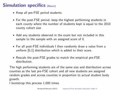
Simulation specifics (Return)
• Keep all pre-FSE period students
• For the post-FSE period, keep the highest performing students ineach county where the number of students kept is equal to the 2010county cohort size
• Add any students observed in the exam but not included in thissample to the sample with an assigned score of 0.
• For all post-FSE individuals I then randomly draw a value from auniform [0,1] distribution which is added to their score.
• Rescale the post-FSE grades to match the empirical pre-FSEdistribution.
The high performing students are of the same size and distribution acrosscounties as the last pre-FSE cohort and all new students are assignedrandom grades and across counties in proportion to actual student bodygrowth.I bootstrap this process 1,000 times.
Brudevold-Newman (2017) Impacts of Free Secondary Education, Slide 77
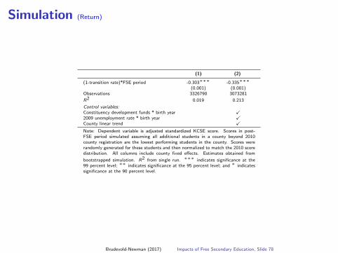
Simulation (Return)
(1) (2)
(1-transition rate)*FSE period -0.303∗∗∗ -0.335∗∗∗(0.001) (0.001)
Observations 3326790 3073281
R2 0.019 0.213
Control variables:Constituency development funds * birth year X2009 unemployment rate * birth year XCounty linear trend X
Note: Dependent variable is adjusted standardized KCSE score. Scores in post-FSE period simulated assuming all additional students in a county beyond 2010county registration are the lowest performing students in the county. Scores wererandomly generated for these students and then normalized to match the 2010 scoredistribution. All columns include county fixed effects. Estimates obtained from
bootstrapped simulation. R2 from single run. ∗∗∗ indicates significance at the99 percent level; ∗∗ indicates significance at the 95 percent level; and ∗ indicatessignificance at the 90 percent level.
Brudevold-Newman (2017) Impacts of Free Secondary Education, Slide 78
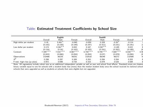
Table: Estimated Treatment Coefficients by School Size
English Swahili MathOverall Male Female Overall Male Female Overall Male Female
High dollar per student 0.18 0.461∗ -0.065 -0.059 0.328 -0.39∗ -0.114 0.32 -0.514∗∗(0.142) (0.238) (0.149) (0.197) (0.311) (0.231) (0.191) (0.27) (0.257)
Low dollar per student 0.174 0.362∗∗ 0.003 0.187 0.587∗∗ -0.185 0.022 0.178 -0.094(0.116) (0.16) (0.163) (0.183) (0.241) (0.262) (0.189) (0.256) (0.259)
Constant 7.309∗∗∗ 7.416∗∗∗ 8.887∗∗∗ 6.740∗∗∗ 6.795∗∗∗ 7.684∗∗∗ 6.838∗∗∗ 6.986∗∗∗ 5.777∗∗∗(0.043) (0.066) (0.054) (0.054) (0.07) (0.078) (0.056) (0.078) (0.08)
Observations 132486 66235 66251 132518 66246 66272 132586 66282 66304
R2 0.298 0.287 0.309 0.263 0.266 0.264 0.203 0.145 0.221F-test: high=low (p-value) 0.972 0.698 0.734 0.316 0.479 0.526 0.569 0.678 0.196
Note: All regressions include cohort size as an additional independent variable as well as year and school fixed effects. Standard errors are clustered at the school level. High (low) dollar per student is abinary variable equal to one for schools with a student body less (more) than the median student body once the school received its national school designation. The sample includes the set of students atschools that were upgraded as well as students at schools that were eligible but not upgraded.
Brudevold-Newman (2017) Impacts of Free Secondary Education, Slide 79

Motivation: impacts on demographic outcomes (Return)
Secondary education may impact demographic outcomes
A variety of potential mechanisms:
• Students may learn about contraceptive methods
• Education may shift preferences towards fewer children
• If having a child precludes schooling, women may delay childbearing
(Becker 1974, Ferre 2009, and Grossman 2006)
These mechanisms likely to delay childbearing/lower fertility levels.
Brudevold-Newman (2017) Impacts of Free Secondary Education, Slide 80

Motivation: impacts on demographic outcomes (Return)
Delaying childbirth in particular could be beneficial
• Early childbearing has been associated with:
I Higher morbidity and mortality (maternal and child)
I Pregnancy related deaths are the largest cause of mortality for 15-19year old females worldwide
I Accounts for 2/3 of deaths in sub-Saharan Africa (15-19 year oldfemales) (Patton et al. The Lancet, 2016)
I Lower educational attainment
I Lower family income
(Ferre 2009 and Schultz 2008)
Mixed evidence on fertility impacts of education:
• Impacts may be conditional on high initial rates
(Osili & Long 2008, Ferre 2009, Keats 2014, Baird et al. 2010, Ozier 2016,
Filmer & Schady 2014, McCrary and Royer 2011)
Brudevold-Newman (2017) Impacts of Free Secondary Education, Slide 81

Motivation: impacts on labor market outcomes (Return)
Secondary education also likely to impact labor market outcomes
Education plays a key role in labor market outcomes (Hanushek and Woßmann
2008, Harmon, Oosterbeek, and Walker 2003, Heckman, Lochner, and Todd 2006, Psacharopoulos
and Patrinos 2004)
• Increased human capital
• Signaling
Quasi-experimental estimates suggest important impacts in developingcountry contexts:
• Education increases income and formality for males in Indonesia andKenya (Duflo 2004, Ozier 2016)
Brudevold-Newman (2017) Impacts of Free Secondary Education, Slide 82

Motivation: impacts on education quality (Return)
Caveat: FSE may also impact student achievement
• The program could dilute existing resources available to studentssuch as:
I Teacher time/effort/attention, Textbooks/desks
• The program could also change the composition of the student body
I Students induced to enroll by free day secondary education aredifferent than students who would enroll in the absence of theprogram
I Possibility of peer effects
Combination yields an unclear impact on student outcomes
• Limited but encouraging results on the impact of free educationprograms on student achievement (Blimpo et al. 2015, Lucas & Mbiti 2012,
Valente 2015)
Brudevold-Newman (2017) Impacts of Free Secondary Education, Slide 83

Conceptual framework (Return)
Consider a two period model where primary school graduates, each withability a, can either:
• Work in both periods or
• Attend secondary school in the first and work in the second period
Secondary school provides a return increasing in ability but costs p
• Trade-off between wage in first period or return in second period
• High ability individuals will want to attend school
• Low ability individuals will want to work
Adapted from Lochner and Monge-Narangjo 2011 and Duflo et al. 2015
Brudevold-Newman (2017) Impacts of Free Secondary Education, Slide 84

Baseline (Return)
0.1
.2.3
.4D
ensi
ty
-4 -2 0 2 4Ability
Lower price increases educational attainment and lowers the averageability of students
Brudevold-Newman (2017) Impacts of Free Secondary Education, Slide 85

Baseline with price decrease (Return)
0.1
.2.3
.4D
ensi
ty
-4 -2 0 2 4Ability
0.1
.2.3
.4D
ensi
ty
-4 -2 0 2 4Ability
Lower price increases educational attainment and lowers the averageability of students
Brudevold-Newman (2017) Impacts of Free Secondary Education, Slide 86

Add credit constraints (Return)
Suppose that students are either from wealthy or poor families
• Students from wealthy families behave as before
• Students from poor families are potentially credit constrained
I Borrowing constraint that depends on ability
I Ex-ante would like to attend subject to the ability threshold
I If the borrowing limit is less than tuition for some high abilityindividuals, they would be precluded from attending school
Brudevold-Newman (2017) Impacts of Free Secondary Education, Slide 87

Credit constraints illustration (Return)
Constrained
0.1
.2.3
.4D
ensi
ty
-4 -2 0 2 4Ability
Lower price increases educational attainment and has an ambiguousimpact on the average ability of students
Brudevold-Newman (2017) Impacts of Free Secondary Education, Slide 88

Credit constraints illustration (Return)
Constrained
0.1
.2.3
.4D
ensi
ty
-4 -2 0 2 4Ability
Constrained
0.1
.2.3
.4D
ensi
ty
-4 -2 0 2 4Ability
Lower price increases educational attainment and has an ambiguousimpact on the average ability of students
Brudevold-Newman (2017) Impacts of Free Secondary Education, Slide 89

Conceptual framework predictions (Return)
Free secondary education will:
• Increase educational attainment
• Have impacts on average student ability contingent on the presenceof credit constraints
I Without credit constraints, the average ability must decrease
I With credit constraints, the average ability could increase, decrease,or stay the same
• Have impacts on academic achievement
I Academic achievement is a combination of ability and resources
I Resource quality decreases, so impact on academic achievement isan indirect test of credit constraints
• Individuals will decrease risky behaviors that would potentiallypreclude further schooling
I High ability individuals need to balance utility from behavior (e.g.sex) against loss from being unable to attend school
Brudevold-Newman (2017) Impacts of Free Secondary Education, Slide 90

Data sources: DHS (Return)
Obs. Mean S.D. Median Min. Max.
Female 13605 0.71 0.46 1 0 1
Age 13605 23.97 3.90 24 18 31
Years of education 13605 10.49 2.35 10 8 19
Completed primary school 13605 1.00 0.00 1 1 1
Attended some secondary school 13605 0.65 0.48 1 0 1
Completed secondary school 13605 0.42 0.49 0 0 1
Female fertility behaviors:
Age at first intercourse 8298 17.72 2.85 18 5 30
Age at first birth 6432 19.54 3.08 19 11 31
Age at first marriage/cohabitation 6097 19.47 3.23 19 10 31
Male fertility behaviors:
Age at first intercourse 3446 16.45 3.38 16 5 30
Age at first marriage/cohabitation 1454 22.46 3.13 23 13 30
Employment sector:
Not working 8499 0.28 0.45 0 0 1
Agricultural work 8499 0.17 0.38 0 0 1
Unskilled work 8499 0.37 0.48 0 0 1
Skilled work 8499 0.18 0.38 0 0 1
Brudevold-Newman (2017) Impacts of Free Secondary Education, Slide 91

Data sources: KNEC (Return)
Administrative Test Scores
Pre-FSE Post-FSE(2008-2010) (2011-2015)
(1) (2)
Number of schools: 5141 7445Public schools: 4346 6213Private schools: 795 1232
Number of test takers per year: 300355 437049Public schools: 262995 384756Private schools: 37360 52294
Number of test takers per school: 88.94 92.32Public schools: 90.23 94.76Private schools: 79.89 74.38
Standardized KCSE score: -0.051 -0.066Public schools: -0.022 -0.050Private schools: -0.254 -0.205
Brudevold-Newman (2017) Impacts of Free Secondary Education, Slide 92

Difference-in-differences (Return)
Identification Assumptions
• Selection bias is attributable to unchanging characteristics
• Common trends
Evidence
• Transition rate potentially determined by regional capacityconstraints, school quality, etc.
• Without large changes, likely to be serially correlated
• Treatment intensities calculated over 2, 10 years are highly correlated
• Common trends (pre-treatment) testable with multiple years ofpre-treatment data
Brudevold-Newman (2017) Impacts of Free Secondary Education, Slide 93
Top Related