


Languages
Pages
Legal


Small World Networks
Adapted from slides by Lada Adamic, UMichigan
Outline
n Small world phenomenon n Milgram’s small world experiment
n Small world network models: n Watts & Strogatz (clustering & short paths) n Kleinberg (geographical) n Watts, Dodds & Newman (hierarchical)
n Small world networks: why do they arise? n efficiency n navigation

NE
MA
Small World Phenomenon: Milgram’s Experiment
Source: undetermined
Instructions: Given a target individual (stockbroker in Boston), pass the message to a person you correspond with who is “closest” to the target.
Outcome: 20% of initiated chains reached target average chain length = 6.5 “Six degrees of separation”
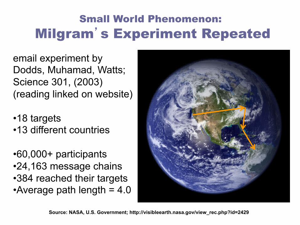
email experiment by Dodds, Muhamad, Watts; Science 301, (2003) (reading linked on website) • 18 targets • 13 different countries • 60,000+ participants • 24,163 message chains • 384 reached their targets • Average path length = 4.0
Small World Phenomenon: Milgram’s Experiment Repeated
Source: NASA, U.S. Government; http://visibleearth.nasa.gov/view_rec.php?id=2429
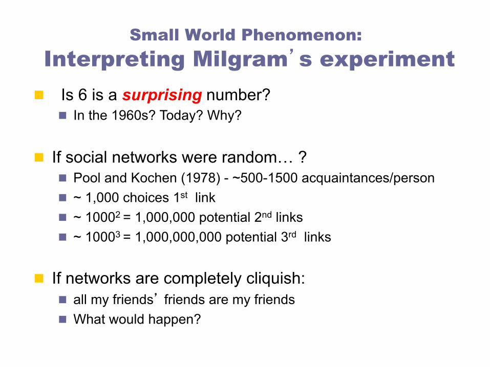
Small World Phenomenon: Interpreting Milgram’s experiment
n Is 6 is a surprising number? n In the 1960s? Today? Why?
n If social networks were random… ? n Pool and Kochen (1978) - ~500-1500 acquaintances/person n ~ 1,000 choices 1st link n ~ 10002 = 1,000,000 potential 2nd links n ~ 10003 = 1,000,000,000 potential 3rd links
n If networks are completely cliquish: n all my friends’ friends are my friends n What would happen?

Small world experiment: Accuracy of distances
n Is 6 an accurate number?
n What bias is introduced by uncompleted chains? n are longer or shorter chains more likely to be completed? n if each person in the chain has 0.5 probability of passing the
letter on, what is the likelihood of a chain being completed n of length 2? n of length 5?

average
95 % confidence interval
Small world experiment accuracy: Attrition rate is approx. constant
prob
abili
ty o
f pas
sing
on
mes
sage
position in chain
Source: An Experimental Study of Search in Global Social Networks: Peter Sheridan Dodds, Roby Muhamad, and Duncan J. Watts (8 August 2003); Science 301 (5634), 827.

n observed chain lengths
n ‘recovered’ histogram of path lengths
inter-country intra-country
Small world experiment accuracy: Estimating true distance distribution
Source: An Experimental Study of Search in Global Social Networks: Peter Sheridan Dodds, Roby Muhamad, and Duncan J. Watts (8 August 2003); Science 301 (5634), 827.
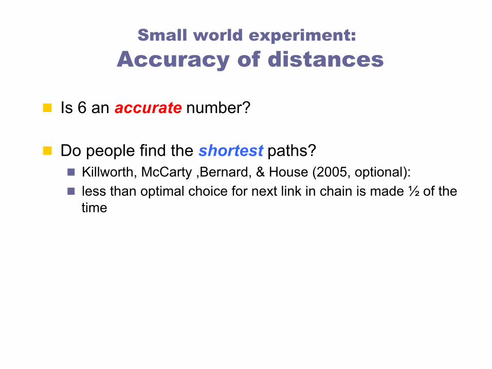
n Is 6 an accurate number?
n Do people find the shortest paths? n Killworth, McCarty ,Bernard, & House (2005, optional): n less than optimal choice for next link in chain is made ½ of the
time
Small world experiment: Accuracy of distances
Current Social Networks n Facebook's data team released two papers in Nov. 2011
n 721 million users with 69 billion friendship links n Average distance of 4.74
n Twitter studies n Sysomos reports the average distance is 4.67 (2010)
n 50% of people are 4 steps apart, nearly everyone is 5 steps or less
n Bakhshandeh et al. (2011) report an average distance of 3.435 among 1,500 random Twitter users
Small world phenomenon: Business applications?
“Social Networking” as a Business: • Facebook, Google+, Orkut, Friendster
entertainment, keeping and finding friends
• LinkedIn: • more traditional networking for jobs
• Spoke, VisiblePath • helping businesses capitalize on existing client relationships

Same pattern: high clustering
low average shortest path
Small world phenomenon: Applicable to other kinds of networks
)ln(network Nl ≈
graph randomnetwork CC >>
" neural network of C. elegans, " semantic networks of languages, " actor collaboration graph " food webs
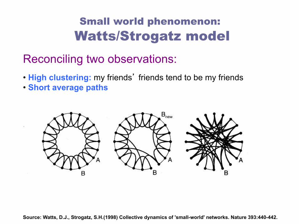
Reconciling two observations: • High clustering: my friends’ friends tend to be my friends • Short average paths
Small world phenomenon: Watts/Strogatz model
Source: Watts, D.J., Strogatz, S.H.(1998) Collective dynamics of 'small-world' networks. Nature 393:440-442.
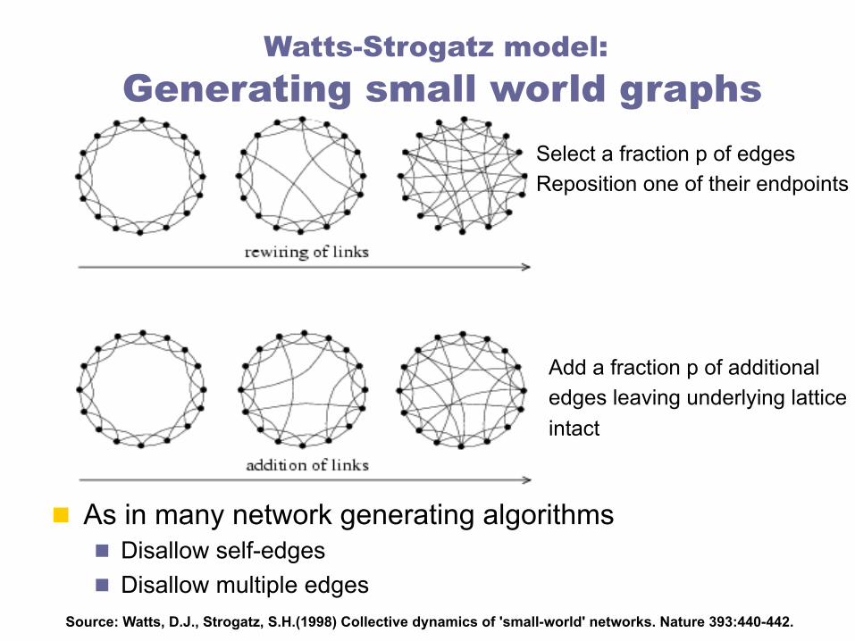
n As in many network generating algorithms n Disallow self-edges n Disallow multiple edges
Select a fraction p of edges Reposition one of their endpoints
Add a fraction p of additional edges leaving underlying lattice intact
Watts-Strogatz model: Generating small world graphs
Source: Watts, D.J., Strogatz, S.H.(1998) Collective dynamics of 'small-world' networks. Nature 393:440-442.
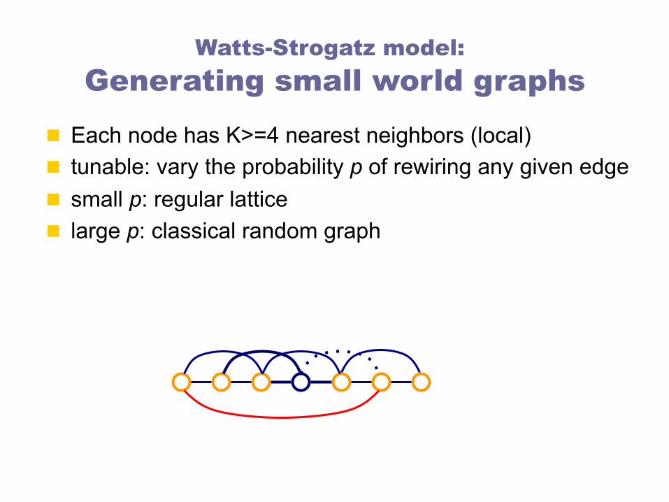
n Each node has K>=4 nearest neighbors (local) n tunable: vary the probability p of rewiring any given edge n small p: regular lattice n large p: classical random graph
Watts-Strogatz model: Generating small world graphs
Watts/Strogatz model: What happens in between?
n Small shortest path means small clustering? n Large shortest path means large clustering? n Through numerical simulation
n As we increase p from 0 to 1 n Fast decrease of mean distance n Slow decrease in clustering

Clustering Coefficient n Clustering coefficient for graph:
n Also known as the “fraction of transitive triples”
# triangles x 3 # connected triples
Each triangle gets counted 3 times
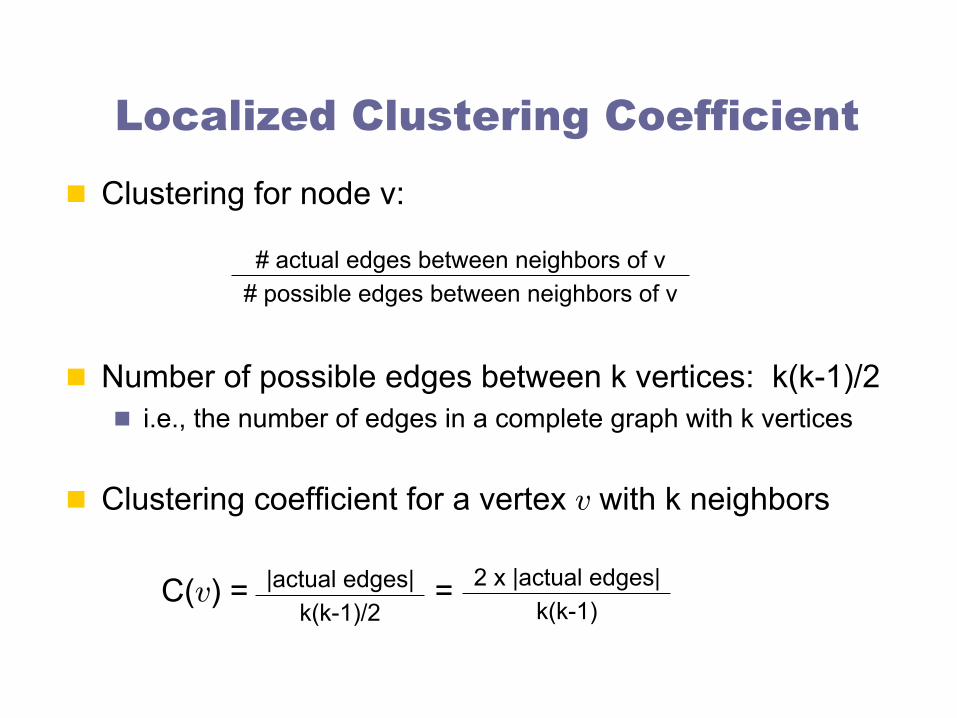
Localized Clustering Coefficient n Clustering for node v:
n Number of possible edges between k vertices: k(k-1)/2 n i.e., the number of edges in a complete graph with k vertices
n Clustering coefficient for a vertex v with k neighbors
C(v) = =
# actual edges between neighbors of v # possible edges between neighbors of v
|actual edges| k(k-1)/2
2 x |actual edges| k(k-1)
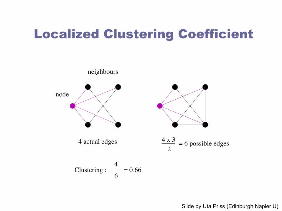
Localized Clustering Coefficient Introduction Watts & Strogatz Scale-free networks Clustering Coe�cient
Clustering Coe�cient
= 0.66
node
neighbours
4 x 3 = 6 possible edges2
4 actual edges
Clustering : 6
4
Copyright Edinburgh Napier University Small World Networks Slide 16/18
Slide by Uta Priss (Edinburgh Napier U)
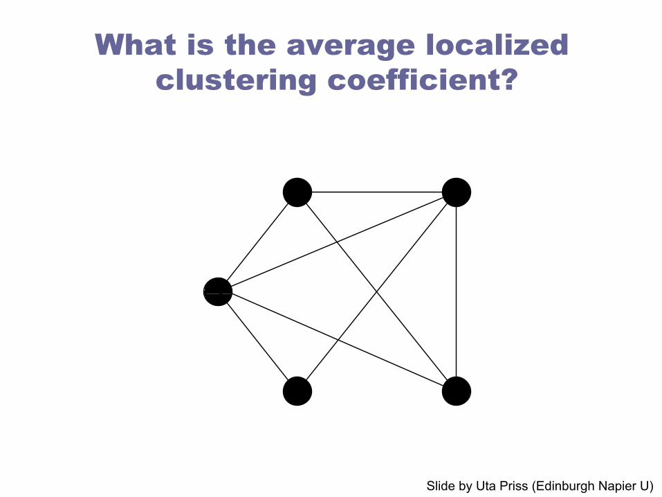
What is the average localized clustering coefficient? Introduction Watts & Strogatz Scale-free networks Clustering Coe�cient
Exercise: Calculate the average clustering coe�cient
Copyright Edinburgh Napier University Small World Networks Slide 17/18
Slide by Uta Priss (Edinburgh Napier U)
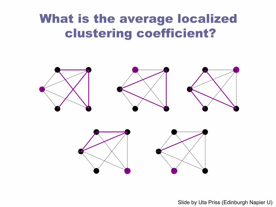
What is the average localized clustering coefficient?
Introduction Watts & Strogatz Scale-free networks Clustering Coe�cient
Exercise: Calculate the average clustering coe�cient
Copyright Edinburgh Napier University Small World Networks Slide 18/18
Slide by Uta Priss (Edinburgh Napier U)

Watts/Strogatz model: Clustering coefficient can be computed for SW model
with rewiring
n The probability that a connected triple stays connected after rewiring n probability that none of the 3 edges were rewired (1-p)3
n probability that edges were rewired back to each other very small, can ignore
n Clustering coefficient = C(p) = C(p=0)*(1-p)3
0.2 0.4 0.6 0.8 1
0.2
0.4
0.6
0.8
1
C(p)/C(0)
p Source: Watts, D.J., Strogatz, S.H.(1998) Collective dynamics of 'small-world' networks. Nature 393:440-442.
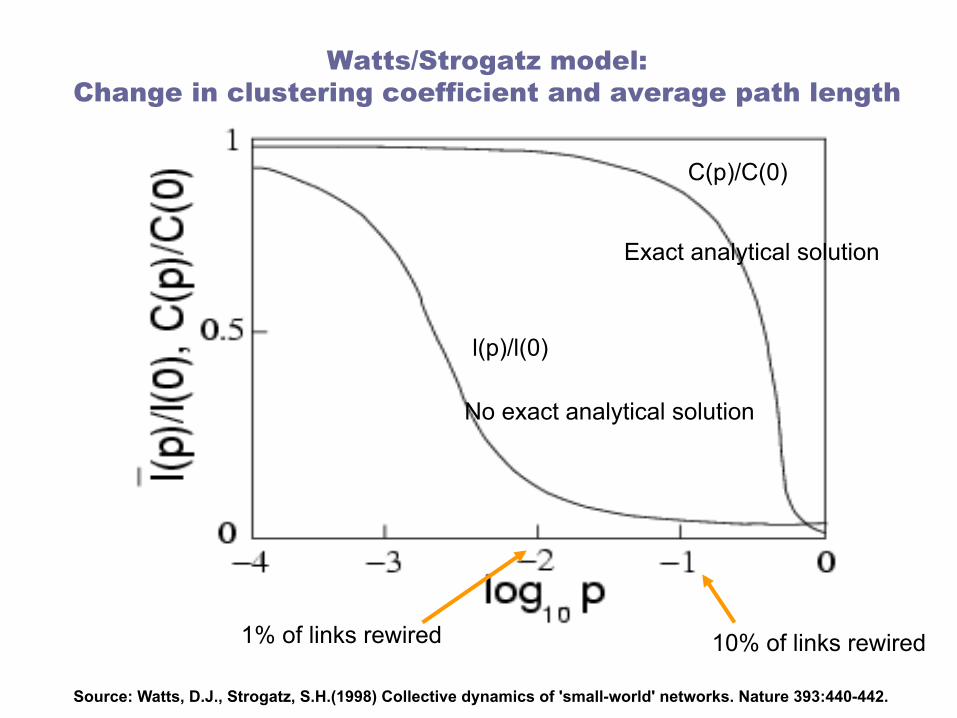
Watts/Strogatz model: Change in clustering coefficient and average path length
as a function of the proportion of rewired edges
l(p)/l(0)
C(p)/C(0)
10% of links rewired 1% of links rewired
No exact analytical solution
Exact analytical solution
Source: Watts, D.J., Strogatz, S.H.(1998) Collective dynamics of 'small-world' networks. Nature 393:440-442.
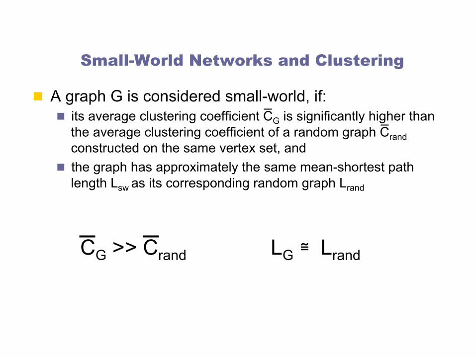
Small-World Networks and Clustering
n A graph G is considered small-world, if: n its average clustering coefficient CG is significantly higher than
the average clustering coefficient of a random graph Crand constructed on the same vertex set, and
n the graph has approximately the same mean-shortest path length Lsw as its corresponding random graph Lrand
CG >> Crand LG ≅ Lrand
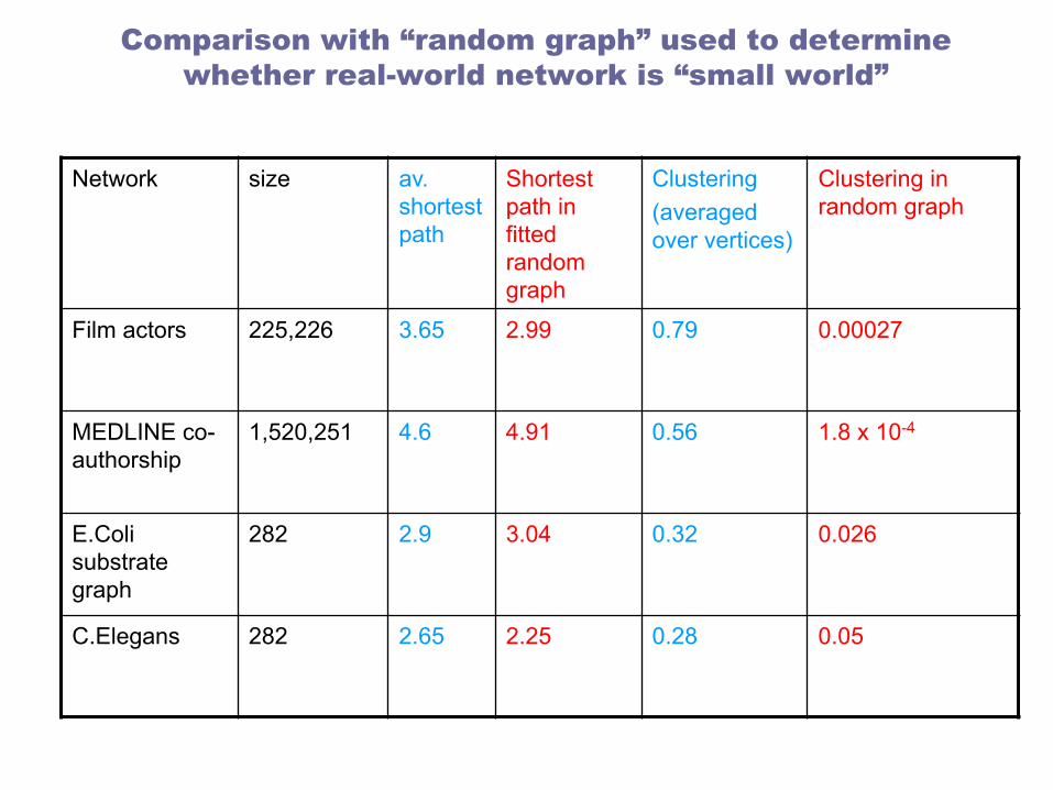
Comparison with “random graph” used to determine whether real-world network is “small world”
Network size av. shortest path
Shortest path in fitted random graph
Clustering (averaged over vertices)
Clustering in random graph
Film actors 225,226 3.65 2.99 0.79 0.00027
MEDLINE co-authorship
1,520,251 4.6 4.91 0.56 1.8 x 10⁻⁴
E.Coli substrate graph
282 2.9 3.04 0.32 0.026
C.Elegans 282 2.65 2.25 0.28 0.05

What features of real social networks are missing from the small world model?
n Long range links not as likely as short range ones n Hierarchical structure / groups n Hubs

Small world networks: Summary
n The world is small! n Watts & Strogatz came up with a simple model to
explain why n Other models incorporate geography and hierarchical
social structure

Extra Material (Not covered in class)
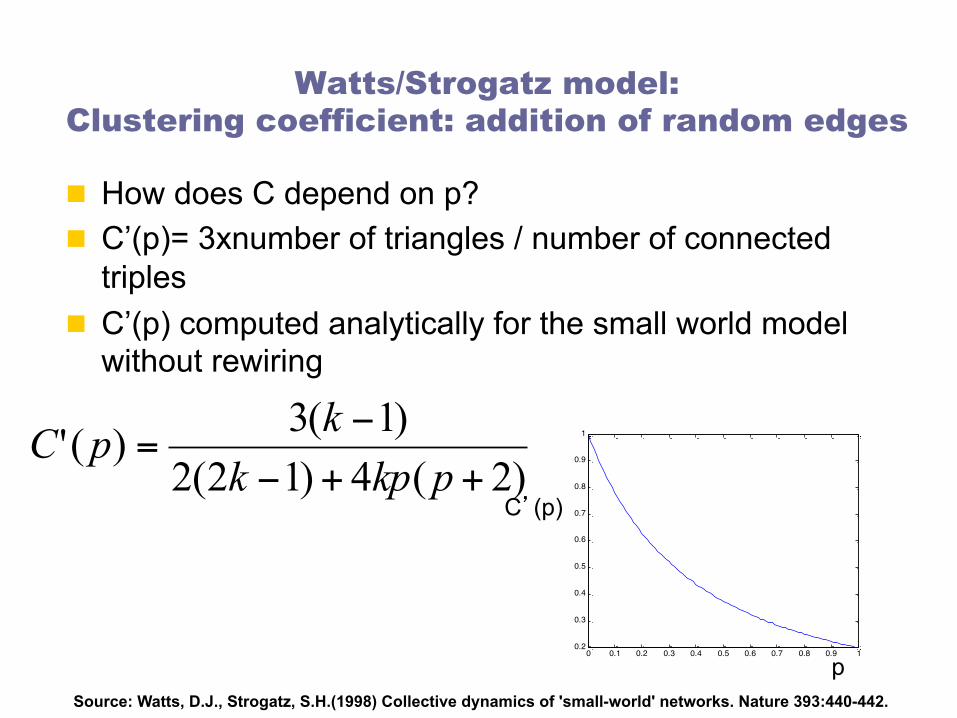
Watts/Strogatz model: Clustering coefficient: addition of random edges
n How does C depend on p? n C’(p)= 3xnumber of triangles / number of connected
triples n C’(p) computed analytically for the small world model
without rewiring
)2(4)12(2)1(3)('
++−
−=
pkpkkpC
0 0.1 0.2 0.3 0.4 0.5 0.6 0.7 0.8 0.9 10.2
0.3
0.4
0.5
0.6
0.7
0.8
0.9
1
p
C’(p)
Source: Watts, D.J., Strogatz, S.H.(1998) Collective dynamics of 'small-world' networks. Nature 393:440-442.

Watts/Strogatz model: Degree distribution
n p=0 delta-function n p>0 broadens the distribution n Edges left in place with probability (1-p) n Edges rewired towards i with probability 1/N
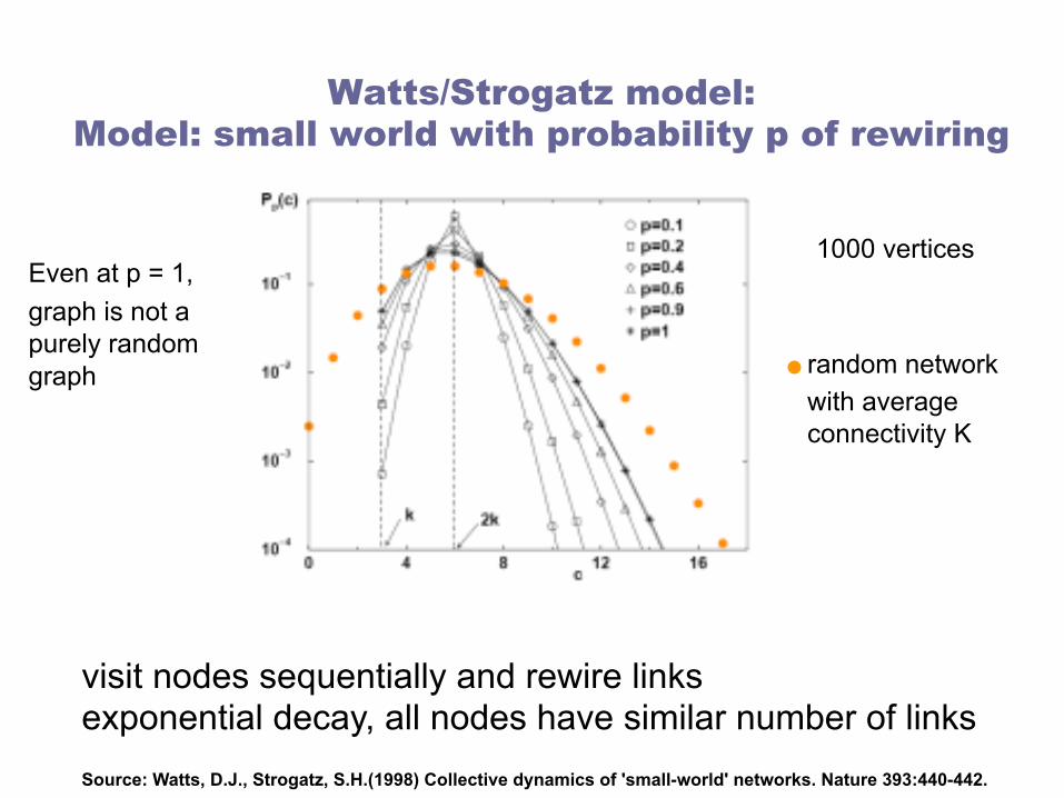
Watts/Strogatz model: Model: small world with probability p of rewiring
visit nodes sequentially and rewire links exponential decay, all nodes have similar number of links
1000 vertices
random network with average connectivity K
Even at p = 1, graph is not a purely random graph
Source: Watts, D.J., Strogatz, S.H.(1998) Collective dynamics of 'small-world' networks. Nature 393:440-442.
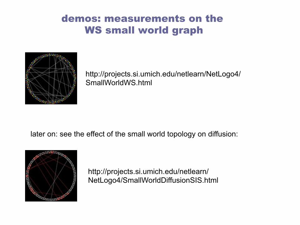
demos: measurements on the WS small world graph
http://projects.si.umich.edu/netlearn/NetLogo4/SmallWorldWS.html
later on: see the effect of the small world topology on diffusion:
http://projects.si.umich.edu/netlearn/NetLogo4/SmallWorldDiffusionSIS.html
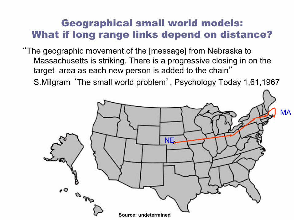
Geographical small world models: What if long range links depend on distance?
“The geographic movement of the [message] from Nebraska to Massachusetts is striking. There is a progressive closing in on the target area as each new person is added to the chain” S.Milgram ‘The small world problem’, Psychology Today 1,61,1967
NE
MA
Source: undetermined

nodes are placed on a lattice and connect to nearest neighbors additional links placed with p(link between u and v) = (distance(u,v))-r
Kleinberg’s geographical small world model
Source: Kleinberg, ‘The Small World Phenomenon, An Algorithmic Perspective’ (Nature 2000).
exponent that will determine navigability
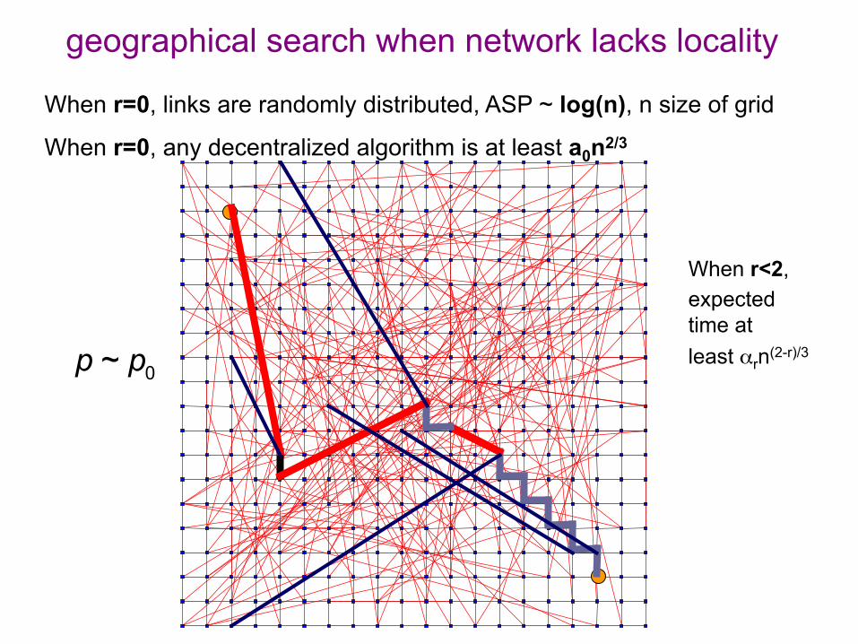
When r=0, links are randomly distributed, ASP ~ log(n), n size of grid
When r=0, any decentralized algorithm is at least a0n2/3
geographical search when network lacks locality
When r<2, expected time at least αrn(2-r)/3
0~p p
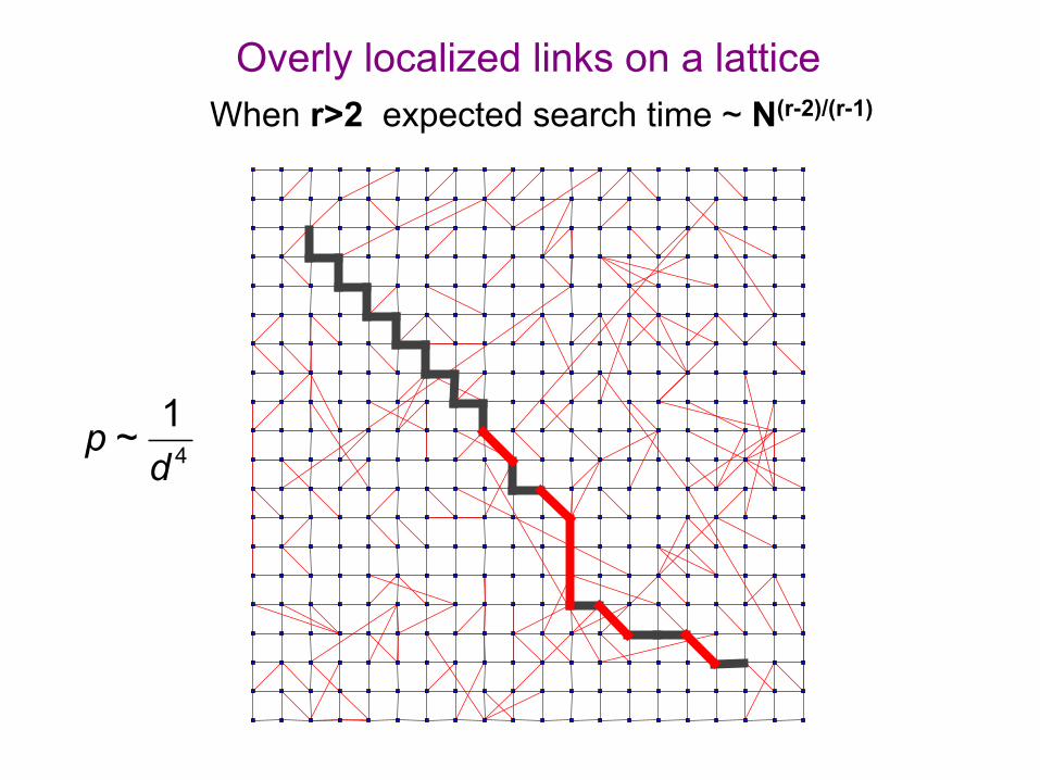
Overly localized links on a lattice When r>2 expected search time ~ N(r-2)/(r-1)
41~pd

When r=2, expected time of a DA is at most C (log N)2
21~pd
geographical small world model Links balanced between long and short range
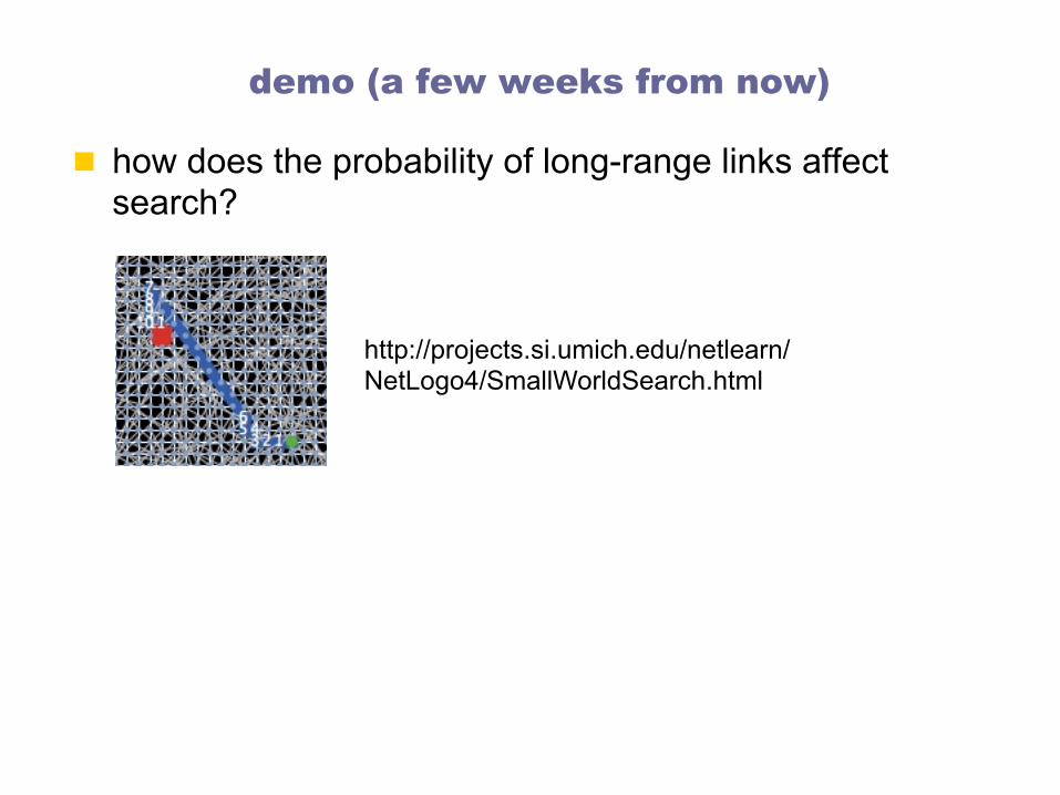
demo (a few weeks from now)
n how does the probability of long-range links affect search?
http://projects.si.umich.edu/netlearn/NetLogo4/SmallWorldSearch.html
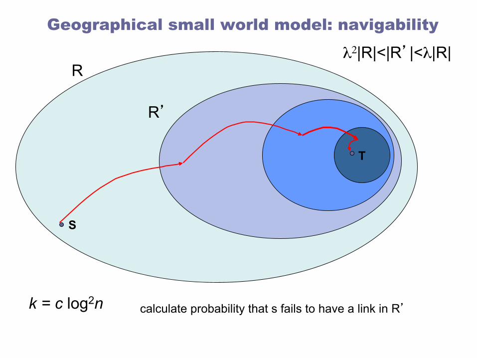
Geographical small world model: navigability
T
S
R λ2|R|<|R’|<λ|R|
k = c log2n calculate probability that s fails to have a link in R’
R’

Source: Kleinberg, ‘Small-World Phenomena and the Dynamics of Information’ NIPS 14, 2001.
Hierarchical network models: Individuals classified into a hierarchy, hij = height of the least common ancestor.
Group structure models: Individuals belong to nested groups q = size of smallest group that v,w belong to
f(q) ~ q-α
ijhijp b α−:
h b=3
e.g. state-county-city-neighborhood industry-corporation-division-group
hierarchical small-world models: Kleinberg
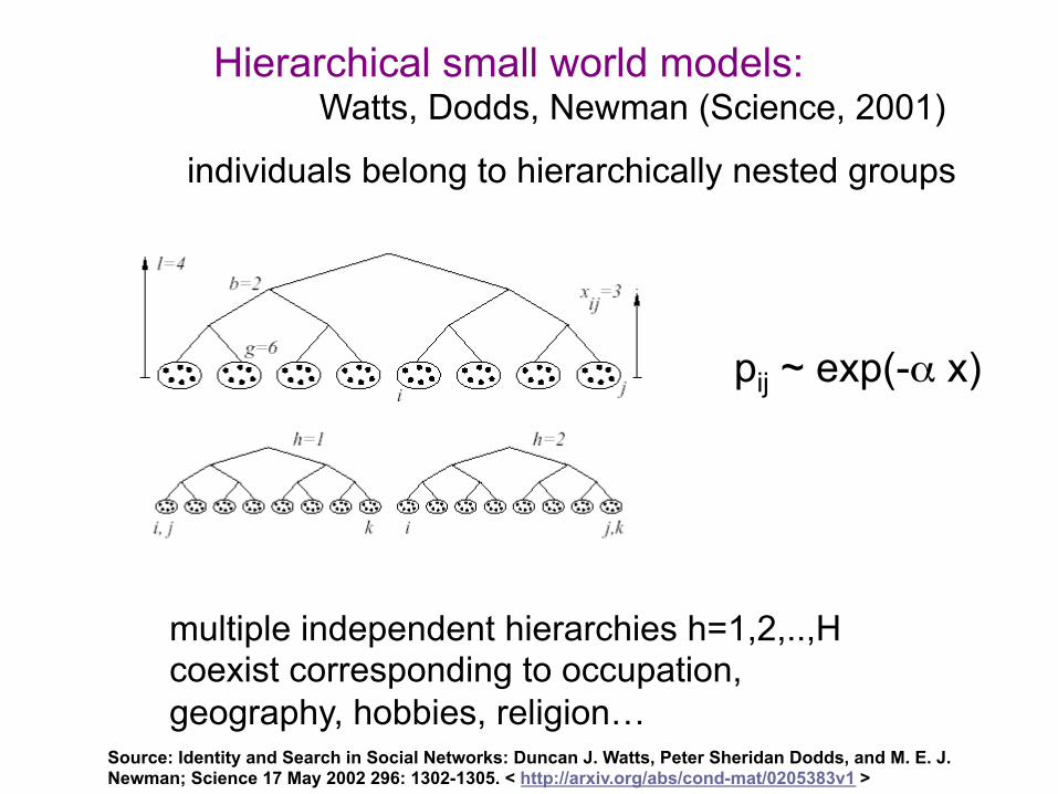
Hierarchical small world models: Watts, Dodds, Newman (Science, 2001)
individuals belong to hierarchically nested groups
multiple independent hierarchies h=1,2,..,H coexist corresponding to occupation, geography, hobbies, religion…
pij ~ exp(-α x)
Source: Identity and Search in Social Networks: Duncan J. Watts, Peter Sheridan Dodds, and M. E. J. Newman; Science 17 May 2002 296: 1302-1305. < http://arxiv.org/abs/cond-mat/0205383v1 >
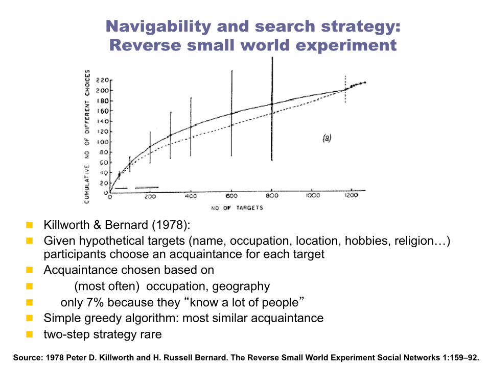
Navigability and search strategy: Reverse small world experiment
n Killworth & Bernard (1978): n Given hypothetical targets (name, occupation, location, hobbies, religion…)
participants choose an acquaintance for each target n Acquaintance chosen based on n (most often) occupation, geography n only 7% because they “know a lot of people” n Simple greedy algorithm: most similar acquaintance n two-step strategy rare
Source: 1978 Peter D. Killworth and H. Russell Bernard. The Reverse Small World Experiment Social Networks 1:159–92.

Successful chains disproportionately used • weak ties (Granovetter) • professional ties (34% vs. 13%) • ties originating at work/college • target's work (65% vs. 40%)
. . . and disproportionately avoided • hubs (8% vs. 1%) (+ no evidence of funnels) • family/friendship ties (60% vs. 83%)
Strategy: Geography -> Work
Navigability and search strategy: Small world experiment @ Columbia

Origins of small worlds: group affiliations

n Assign properties to nodes (e.g. spatial location, group membership)
n Add or rewire links according to some rule n optimize for a particular property (simulated annealing) n add links with probability depending on property of existing
nodes, edges (preferential attachment, link copying) n simulate nodes as agents ‘deciding’ whether to rewire or add
links
Origins of small worlds: other generative models

Origins of small worlds: efficient network example trade-off between wiring and connectivity
n E is the ‘energy’ cost we are trying to minimize n L is the average shortest path in ‘hops’ n W is the total length of wire used
Small worlds: How and Why, Nisha Mathias and Venkatesh Gopal
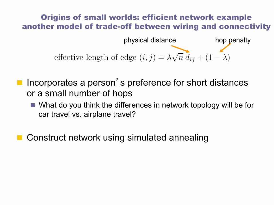
n Incorporates a person’s preference for short distances or a small number of hops n What do you think the differences in network topology will be for
car travel vs. airplane travel?
n Construct network using simulated annealing
physical distance hop penalty
Origins of small worlds: efficient network example another model of trade-off between wiring and connectivity

Air traffic networks
Image: Aaron Koblin http://aaronkoblin.com/gallery/index.html
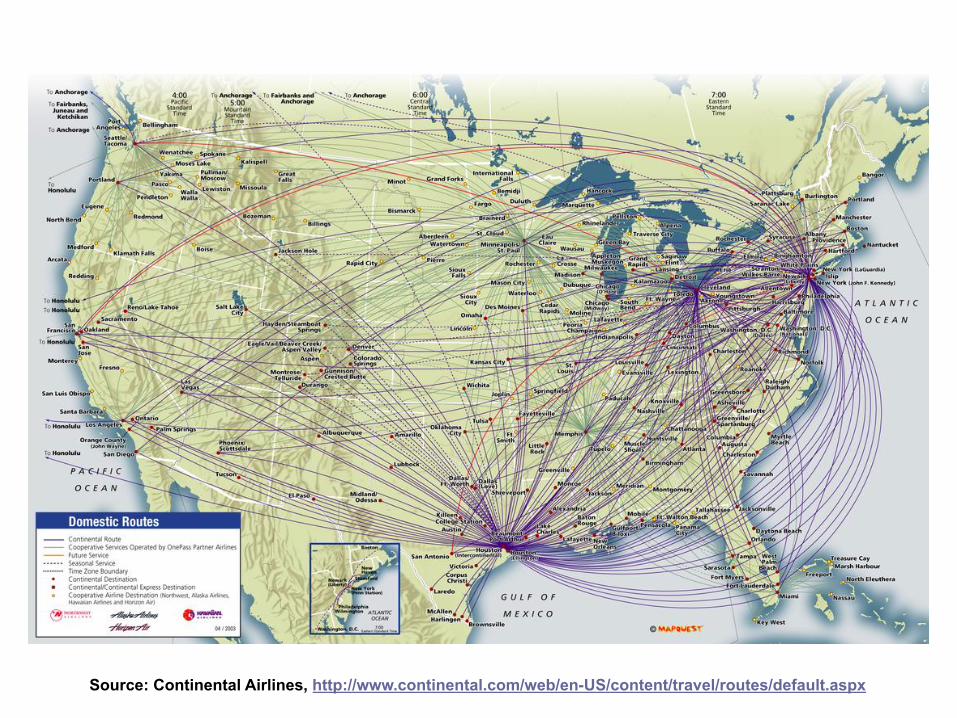
Source: Continental Airlines, http://www.continental.com/web/en-US/content/travel/routes/default.aspx

Source: http://maps.google.com
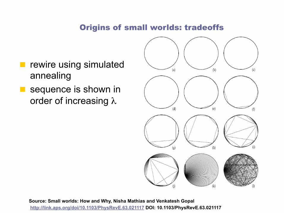
n rewire using simulated annealing
n sequence is shown in order of increasing λ
Origins of small worlds: tradeoffs
Source: Small worlds: How and Why, Nisha Mathias and Venkatesh Gopal http://link.aps.org/doi/10.1103/PhysRevE.63.021117 DOI: 10.1103/PhysRevE.63.021117

n same networks, but the vertices are allowed to move using a spring layout algorithm
n wiring cost associated with the physical distance between nodes
Origins of small worlds: tradeoffs
Source: Small worlds: How and Why, Nisha Mathias and Venkatesh Gopal http://link.aps.org/doi/10.1103/PhysRevE.63.021117 DOI: 10.1103/PhysRevE.63.021117
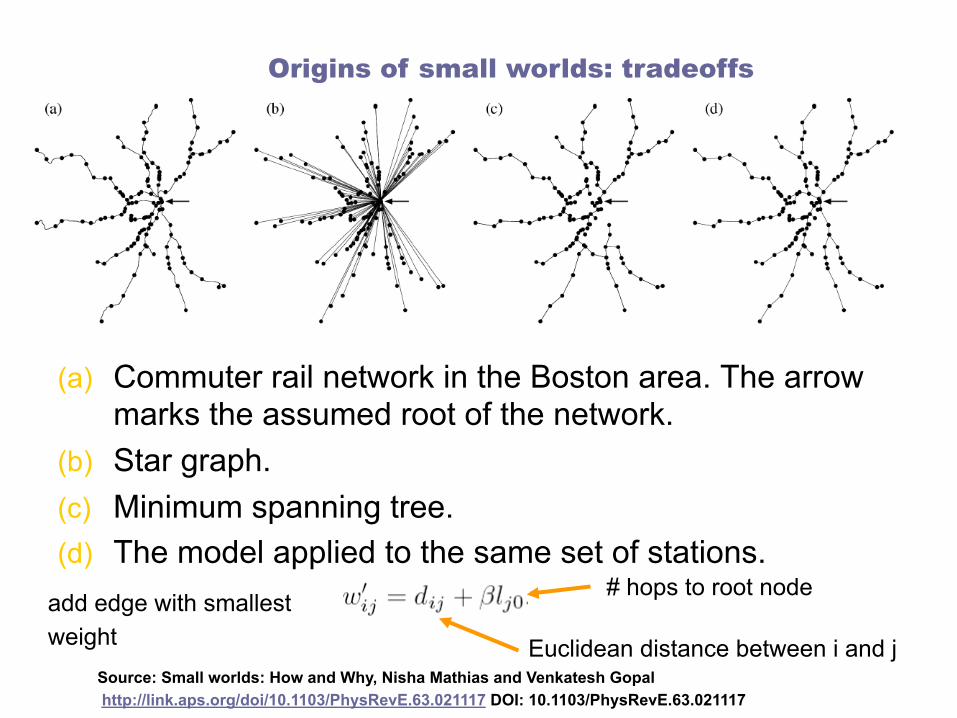
(a) Commuter rail network in the Boston area. The arrow marks the assumed root of the network.
(b) Star graph. (c) Minimum spanning tree. (d) The model applied to the same set of stations.
add edge with smallest weight Euclidean distance between i and j
# hops to root node
Origins of small worlds: tradeoffs
Source: Small worlds: How and Why, Nisha Mathias and Venkatesh Gopal http://link.aps.org/doi/10.1103/PhysRevE.63.021117 DOI: 10.1103/PhysRevE.63.021117

Source: The Spatial Structure of Networks, M. T. Gastner and M. E.J. Newman http://www.springerlink.com/content/p26t67882668514q DOI: 10.1140/epjb/e2006-00046-8

Roads Air routes
Source: The Spatial Structure of Networks, M. T. Gastner and M. E.J. Newman http://www.springerlink.com/content/p26t67882668514q DOI: 10.1140/epjb/e2006-00046-8
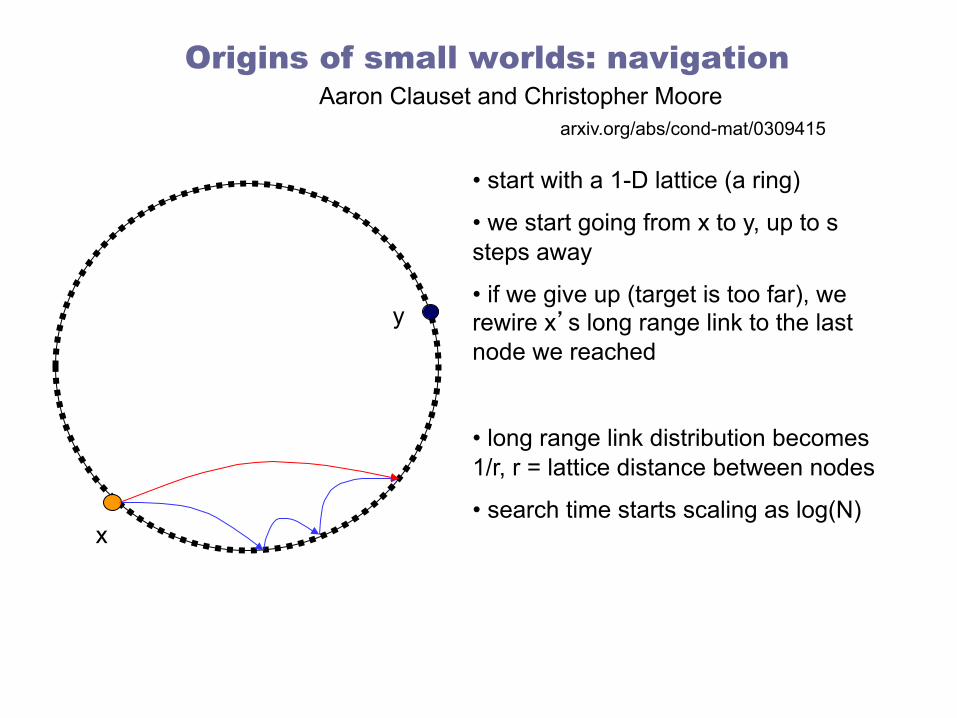
Origins of small worlds: navigation Aaron Clauset and Christopher Moore
arxiv.org/abs/cond-mat/0309415
• start with a 1-D lattice (a ring)
• we start going from x to y, up to s steps away
• if we give up (target is too far), we rewire x’s long range link to the last node we reached
• long range link distribution becomes 1/r, r = lattice distance between nodes
• search time starts scaling as log(N) x
y
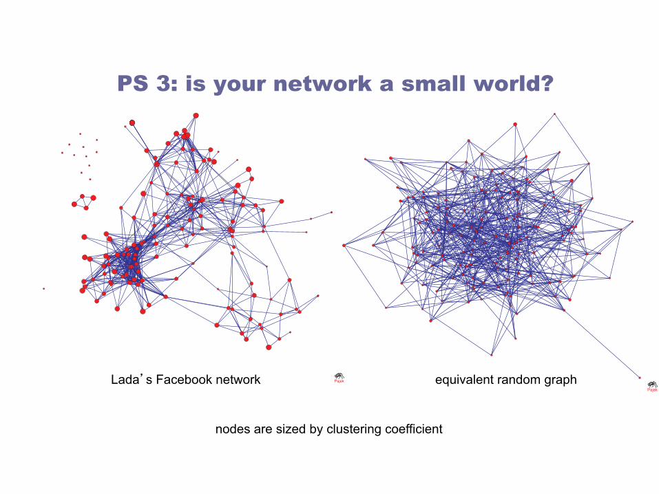
PS 3: is your network a small world?
Pajek
Pajek
Lada’s Facebook network equivalent random graph
nodes are sized by clustering coefficient
Small world networks: Summary
n The world is small! n Watts & Strogatz came up with a simple model to explain
why n Other models incorporate geography and hierarchical
social structure n Small worlds may evolve from different constraints
(navigation, constraint optimization, group affiliation)
Top Related