Sales Forecasting for Airline

Submitted By:Anurag ShandilyaAnkur KhandelwalPullahbhatla AuproopSrikanth MallyaShekhar SinhaSoham Mukhopadhyay

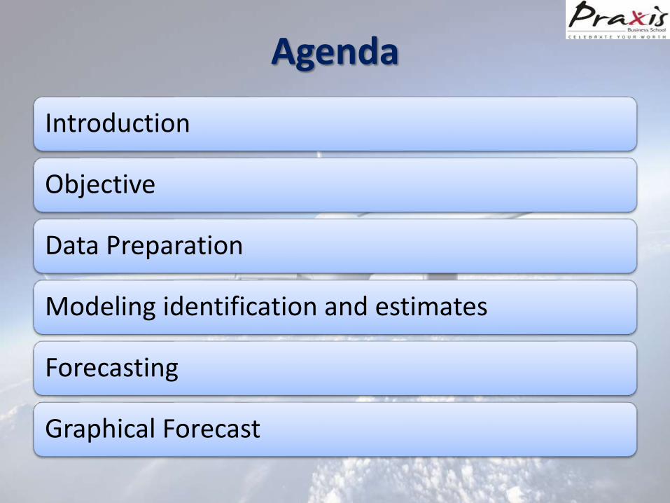
Agenda

Introduction

Objective

Data Preparation

Modeling identification and estimates

Forecasting

Graphical Forecast

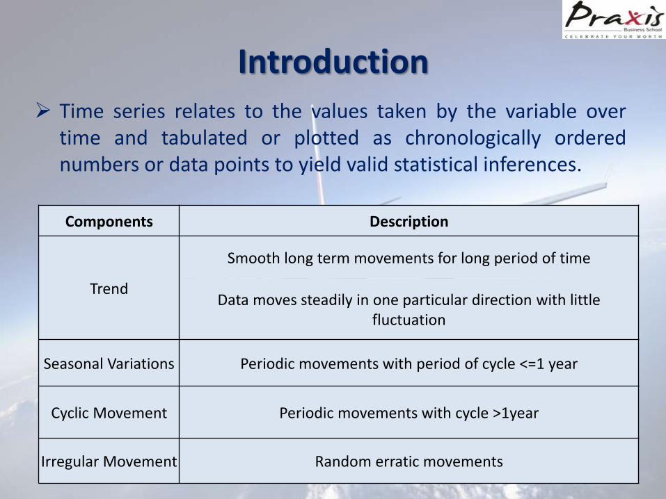
Introduction Time series relates to the values taken by the variable over

time and tabulated or plotted as chronologically orderednumbers or data points to yield valid statistical inferences.

Components Description

Trend

Smooth long term movements for long period of time

Data moves steadily in one particular direction with little fluctuation

Seasonal Variations Periodic movements with period of cycle <=1 year

Cyclic Movement Periodic movements with cycle >1year

Irregular Movement Random erratic movements

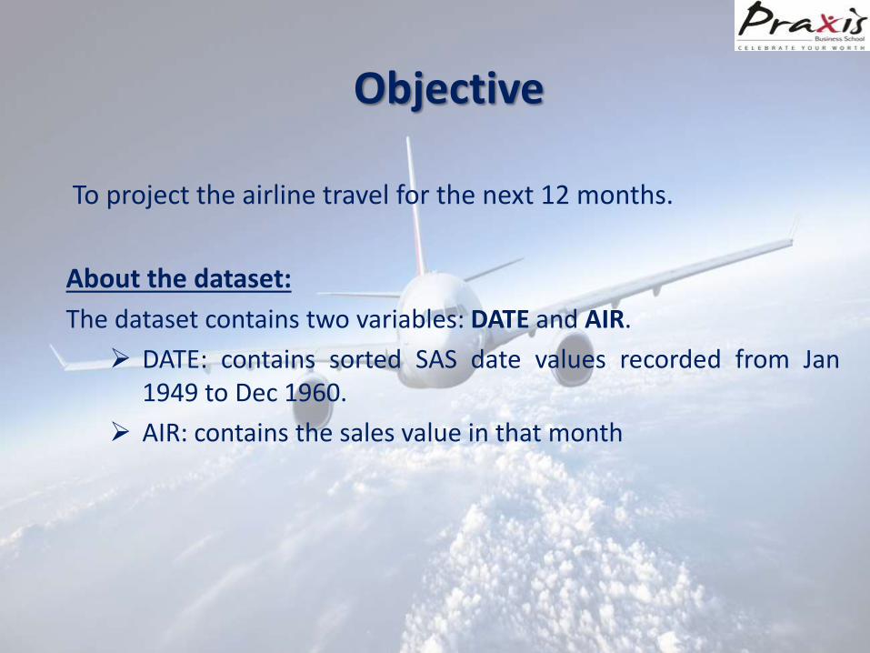
Objective

To project the airline travel for the next 12 months.

About the dataset:

The dataset contains two variables: DATE and AIR.

DATE: contains sorted SAS date values recorded from Jan1949 to Dec 1960.

AIR: contains the sales value in that month

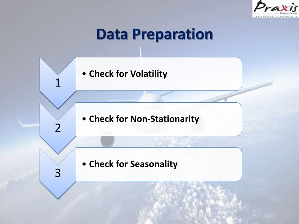
Data Preparation

1• Check for Volatility

2• Check for Non-Stationarity

3• Check for Seasonality

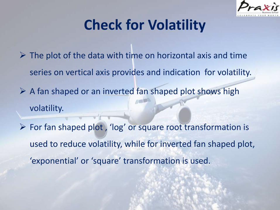
Check for Volatility

The plot of the data with time on horizontal axis and time

series on vertical axis provides and indication for volatility.

A fan shaped or an inverted fan shaped plot shows high

volatility.

For fan shaped plot , ‘log’ or square root transformation is

used to reduce volatility, while for inverted fan shaped plot,

‘exponential’ or ‘square’ transformation is used.

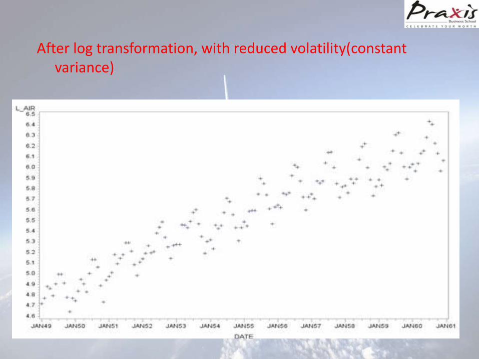
After log transformation, with reduced volatility(constant variance)

Check for Non-Stationarity

• A non stationary data is completely memory less with nofixed patterns. Such a data can’t be used for forecasting

• Augmented Dickey Fuller Test (ADF) used to check the non-stationarity of data.

• Non-Stationarity can be removed by differencing.

• Data was found to be non-stationary & hence, differencingof log transformed data was done to make data stationary.

Check for seasonality:

The Auto Correlation function (ACF) gives the correlation

between y[t]-y[t-s] where ‘s’ is the period of lag.

If ACF gives high values at fixed interval that interval can be

considered as the period of seasonality. A differencing of

same order will depersonalize the data.

From the output of ACF it can be observed that the period

of seasonality is 12 years.

Model Identification and estimation

Depending upon the number of future time points to be forecasted

, we set aside few of the most recent time points as the validation

sample.

The rest of the data which is development sample, is used to

generate forecasts for the different models.

MINIC(Minimum Information Criteria) generate the minimum

BIC(Bayesian Information Criteria) model after exploring all the

possible combinations of Auto Regressive and Moving Average lags

from 0 to 5.

Model Identification and estimation

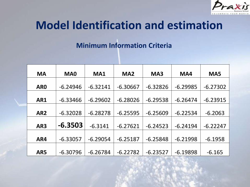
MA MA0 MA1 MA2 MA3 MA4 MA5

AR0 -6.24946 -6.32141 -6.30667 -6.32826 -6.29985 -6.27302

AR1 -6.33466 -6.29602 -6.28026 -6.29538 -6.26474 -6.23915

AR2 -6.32028 -6.28278 -6.25595 -6.25609 -6.22534 -6.2063

AR3 -6.3503 -6.3141 -6.27621 -6.24523 -6.24194 -6.22247

AR4 -6.33057 -6.29054 -6.25187 -6.25848 -6.21998 -6.1958

AR5 -6.30796 -6.26784 -6.22782 -6.23527 -6.19898 -6.165

Minimum Information Criteria

Model Identification and estimation

By observation we can see that minimum of the matrix is

the value -6.3503 corresponding to AR3 and MA 0

location(i.e. p=0 & =3).

We consider all the models in the neighborhood of this

model and for each of them generate AIC(Akaike

Information Criteria) and SBC (Schwartz Bayesian Criteria)

and calculate and average of them.

We select top 6-7 models based on relatively lower value of

the average and for each of them generate forecasts.

Forecasting

The forecasts generated (for the year 1960) for each of the 6

combination selected from AIC & SBC separately compared

with the actual values of the same time point stored in the

dataset.

‘MAPE’ (Mean Absolute Percentage Error) is calculated for 6

forecasted values for the year 1960.

Lowest MAPE value comes out to be for p=0 and q=3, hence

final forecasting will be done using this model.

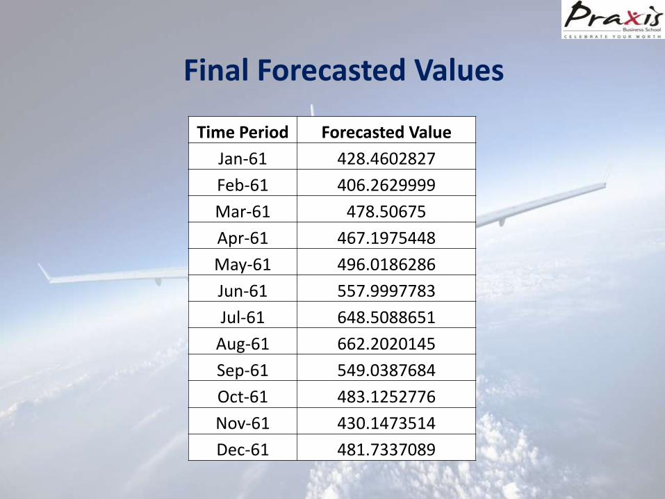
Final Forecasted Values

Time Period Forecasted Value

Jan-61 428.4602827

Feb-61 406.2629999

Mar-61 478.50675

Apr-61 467.1975448

May-61 496.0186286

Jun-61 557.9997783

Jul-61 648.5088651

Aug-61 662.2020145

Sep-61 549.0387684

Oct-61 483.1252776

Nov-61 430.1473514

Dec-61 481.7337089

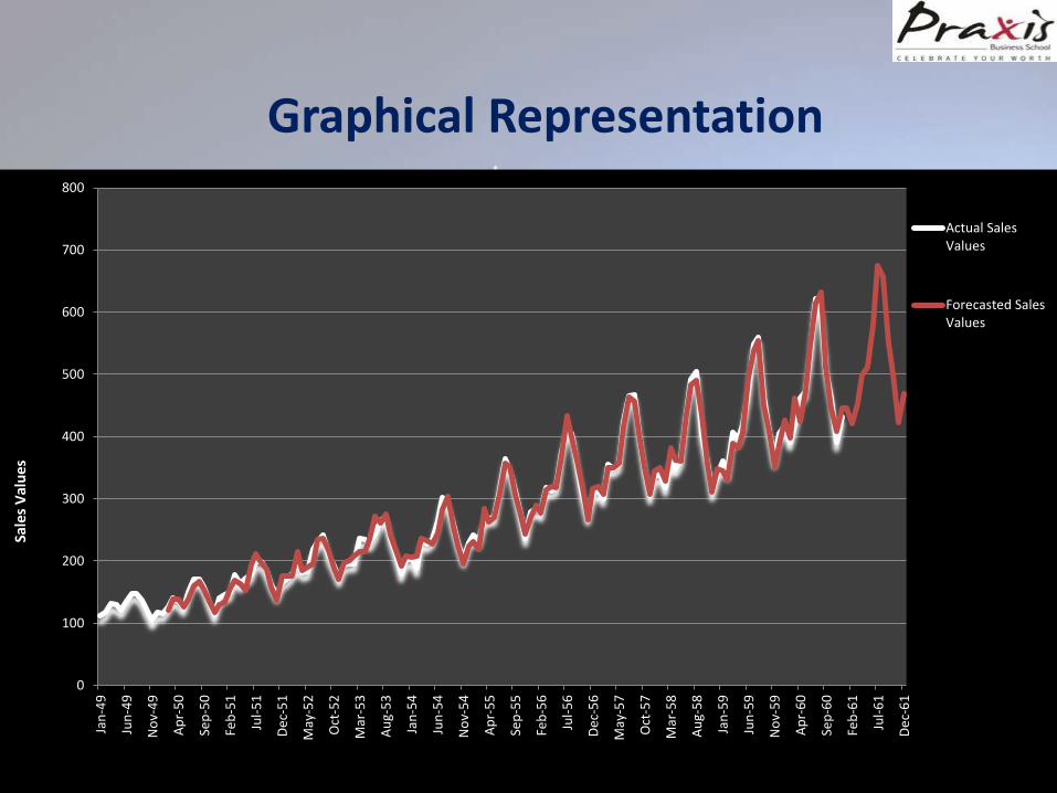
Graphical Representation

0

100

200

300

400

500

600

700

800

Jan

-49

Jun

-49

No

v-4

9

Ap

r-5

0

Sep

-50

Feb

-51

Jul-

51

De

c-5

1

May

-52

Oct

-52

Mar

-53

Au

g-5

3

Jan

-54

Jun

-54

No

v-5

4

Ap

r-5

5

Sep

-55

Feb

-56

Jul-

56

De

c-5

6

May

-57

Oct

-57

Mar

-58

Au

g-5

8

Jan

-59

Jun

-59

No

v-5

9

Ap

r-6

0

Sep

-60

Feb

-61

Jul-

61

De

c-6

1

Actual SalesValues

Forecasted SalesValues

Sale

s V

alu

es

Appendix

AIC, SBC, MAP excel sheet is attached in mail

“SAS code for forecasting”