


Languages
Pages
Legal

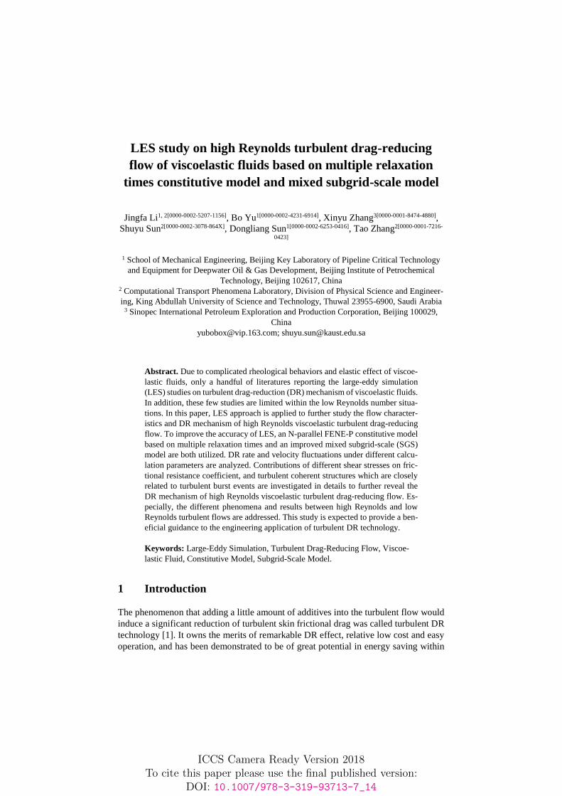
LES study on high Reynolds turbulent drag-reducing
flow of viscoelastic fluids based on multiple relaxation
times constitutive model and mixed subgrid-scale model
Jingfa Li1, 2[0000-0002-5207-1156], Bo Yu1[0000-0002-4231-6914], Xinyu Zhang3[0000-0001-8474-4880],
Shuyu Sun2[0000-0002-3078-864X], Dongliang Sun1[0000-0002-6253-0416], Tao Zhang2[0000-0001-7216-
0423]
1 School of Mechanical Engineering, Beijing Key Laboratory of Pipeline Critical Technology
and Equipment for Deepwater Oil & Gas Development, Beijing Institute of Petrochemical
Technology, Beijing 102617, China 2 Computational Transport Phenomena Laboratory, Division of Physical Science and Engineer-
ing, King Abdullah University of Science and Technology, Thuwal 23955-6900, Saudi Arabia 3 Sinopec International Petroleum Exploration and Production Corporation, Beijing 100029,
China
[email protected]; [email protected]
Abstract. Due to complicated rheological behaviors and elastic effect of viscoe-
lastic fluids, only a handful of literatures reporting the large-eddy simulation
(LES) studies on turbulent drag-reduction (DR) mechanism of viscoelastic fluids.
In addition, these few studies are limited within the low Reynolds number situa-
tions. In this paper, LES approach is applied to further study the flow character-
istics and DR mechanism of high Reynolds viscoelastic turbulent drag-reducing
flow. To improve the accuracy of LES, an N-parallel FENE-P constitutive model
based on multiple relaxation times and an improved mixed subgrid-scale (SGS)
model are both utilized. DR rate and velocity fluctuations under different calcu-
lation parameters are analyzed. Contributions of different shear stresses on fric-
tional resistance coefficient, and turbulent coherent structures which are closely
related to turbulent burst events are investigated in details to further reveal the
DR mechanism of high Reynolds viscoelastic turbulent drag-reducing flow. Es-
pecially, the different phenomena and results between high Reynolds and low
Reynolds turbulent flows are addressed. This study is expected to provide a ben-
eficial guidance to the engineering application of turbulent DR technology.
Keywords: Large-Eddy Simulation, Turbulent Drag-Reducing Flow, Viscoe-
lastic Fluid, Constitutive Model, Subgrid-Scale Model.
1 Introduction
The phenomenon that adding a little amount of additives into the turbulent flow would
induce a significant reduction of turbulent skin frictional drag was called turbulent DR
technology [1]. It owns the merits of remarkable DR effect, relative low cost and easy
operation, and has been demonstrated to be of great potential in energy saving within
ICCS Camera Ready Version 2018To cite this paper please use the final published version:
DOI: 10.1007/978-3-319-93713-7_14
2
the long-distance liquid transportation and circulation systems. To better apply this
technique, the turbulent DR mechanism should be investigated intensively. In recent
two decades, the rapid development of computer technology brought great changes to
the studies on turbulent flow, where numerical simulation has become an indispensable
approach. Among the commonly-used numerical approaches for simulation of turbu-
lent flow, the computational workload of LES is smaller than that of direct numerical
simulation (DNS) while the obtained information is much more comprehensive and
detailed than that of Reynolds-averaged Navier-Stokes (RANS) simulation. It makes a
more detailed but time-saving investigation on the turbulent flow with relatively high
Reynolds number possible. Therefore, LES has a brilliant prospective in the research
of turbulent flow especially with viscoelastic fluids.
Different from the LES of Newtonian fluid, a constitutive model describing the re-
lationship between elastic stress and deformation tensor should be established first for
the LES of viscoelastic fluid. An accurate constitutive model that matches the physical
meaning is a critical guarantee to the reliability of LES. Up to now most of the consti-
tutive models for viscoelastic fluid, such as generalized Maxwell model [2], Oldroyd-
B model [3, 4], Giesekus model [5] and FENE-P model [6], were all built on polymer
solutions because the long-chain polymer is the most extensively used DR additive in
engineering application. Compared with Maxwell and Oldroyd-B models, the Giesekus
model as well as FENE-P model can characterize the shear thinning behavior of poly-
mer solutions much better and thus they are adopted by most researchers. However, it
is reported in some studies that the apparent viscosity calculated with Giesekus model
and FENE-P model still deviated from experimental data to some extent, indicating an
unsatisfactory accuracy [7]. Inspired by the fact that constitutive model with multiple
relaxation times can better describe the relaxation-deformation of microstructures
formed in viscoelastic fluid, an N-parallel FENE-P model based on multiple relaxation
times was proposed in our recent work [8]. The comparison with experimental data
shows the N-parallel FENE-P model can further improve the computational accuracy
of rheological characteristics, such as apparent viscosity and first normal stress differ-
ence.
For the LES of viscoelastic fluid, the effective SGS model is still absent. To the best
of our knowledge, only a handful of researches have studied this problem. In 2010,
Thais et al. [9] first adopted temporal approximate deconvolution model (TADM) to
perform LES on the turbulent channel flow of polymer solutions, in which the filtered
governing equation of LES was derived. Wang et al. [10] made a comparison between
approximate deconvolution model (ADM) and TADM. It was found that the TADM
was more suitable to LES study on viscoelastic turbulent channel flow. In 2015, com-
prehensively considering the characteristics of both momentum equations and consti-
tutive equations of viscoelastic fluid, Li et al. [11] put forward a mixed SGS model
called MCT based on coherent-structure Smagorinsky model (CSM) [12] and TADM.
The forced isotropic turbulent flow of polymer solution and turbulent channel flow of
surfactant solution were both simulated by using MCT. The calculation results such as
turbulent energy spectrum, two-point spanwise correlations, and vortex tube structures
agreed well with the DNS database. Although MCT made an important step to the
mixed SGS model coupling spatial filtering and temporal filtering altogether, it was
ICCS Camera Ready Version 2018To cite this paper please use the final published version:
DOI: 10.1007/978-3-319-93713-7_14

3
still limited by its spatial SGS model—CSM, with which an excessive energy dissipa-
tion is observed near the channel wall. In our recent work [13] we improved the CSM
and proposed an improved mixed SGS model named MICT based on ICSM and
TADM. Simulation results, for instance, DR rate, streamwise mean velocity, two-point
spanwise correlations, were compared to demonstrate a better accuracy of MICT than
conventional SGS models.
Regarding the turbulent flow itself, due to the intrinsic complexity and limitation of
numerical approaches, together with the complicated non-Newtonian behaviors of vis-
coelastic fluid, the understanding of turbulent DR mechanism is generally limited
within flows with relatively low Reynolds number. For the high Reynolds viscoelastic
turbulent flows which are commonly seen in industry and engineering, the turbulent
DR mechanism is still far from fully understood, which makes the quantitative guidance
on engineering application of DR technology inadequate. Therefore, deeper studies
need to be performed on the high Reynolds turbulent drag-reducing flows.
With above background and based on our recent studies on the constitutive model
and SGS model of viscoelastic fluid, we apply the LES to further explore the turbulent
DR mechanism of high Reynolds viscoelastic turbulent flows in this study. The remain-
der of this paper is organized as follows. In Section 2, the N-parallel FENE-P model
based on multiple relaxation times and the improved mixed SGS model MICT are
briefly introduced. Then the governing equation of LES for viscoelastic turbulent drag-
reducing channel flow is presented accordingly. Section 3 of this paper is devoted to
describing the LES approach adopted in this paper. In Section 4, the flow characteristics
and DR mechanism of high Reynolds turbulent drag-reducing channel flow are deeply
studied and analyzed. In the final Section the most important findings of this study are
summarized.
2 Governing equation of LES for viscoelastic turbulent drag-
reducing flows
2.1 The N-parallel FENE-P constitutive model
To improve the computational accuracy of constitutive model needed for LES of vis-
coelastic turbulent flows, an N-parallel FENE-P model based on multiple relaxation
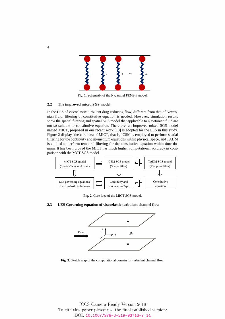
times was proposed in our recent work [8]. As shown in Fig. 1, the core idea of the
proposed constitutive model is to connect N FENE-P models, which has single relaxa-
tion time, in parallel. With this parallel FENE-P model, stress-strain relationships of
different microstructures formed in viscoelastic fluid are more truly modelled compared
with the conventional FENE-P model, and it can better characterize the anisotropy of
the relaxation-deformation in viscoelastic fluid. Comparative results indicate the N-
parallel FENE-P constitutive model can better satisfy the relaxation-deformation pro-
cess of microstructures, and characterize the rheological behaviors of viscoelastic fluid
with much higher accuracy.
ICCS Camera Ready Version 2018To cite this paper please use the final published version:
DOI: 10.1007/978-3-319-93713-7_14
4
Fig. 1. Schematic of the N-parallel FENE-P model.
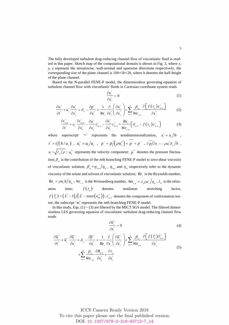
2.2 The improved mixed SGS model
In the LES of viscoelastic turbulent drag-reducing flow, different from that of Newto-
nian fluid, filtering of constitutive equation is needed. However, simulation results
show the spatial filtering and spatial SGS model that applicable to Newtonian fluid are
not so suitable to constitutive equation. Therefore, an improved mixed SGS model
named MICT, proposed in our recent work [13] is adopted for the LES in this study.
Figure 2 displays the core idea of MICT, that is, ICSM is employed to perform spatial
filtering for the continuity and momentum equations within physical space, and TADM
is applied to perform temporal filtering for the constitutive equation within time-do-
main. It has been proved the MICT has much higher computational accuracy in com-
parison with the MCT SGS model.
Fig. 2. Core idea of the MICT SGS model.
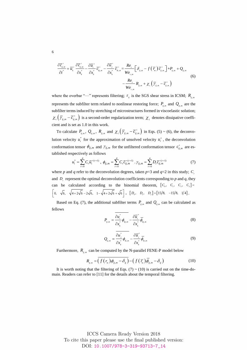
2.3 LES Governing equation of viscoelastic turbulent channel flow
Fig. 3. Sketch map of the computational domain for turbulent channel flow.
MICT SGS model
(Spatial-Temporal filter)
ICSM SGS model
(Spatial filter)
LES governing equations
of viscoelastic turbulence
Continuity and
momentum Eqs. (Spatial fil-
TADM SGS model
(Temporal filter)
Constitutive
equation
x
y
z
2h Flow
ICCS Camera Ready Version 2018To cite this paper please use the final published version:
DOI: 10.1007/978-3-319-93713-7_14
5
The fully developed turbulent drag-reducing channel flow of viscoelastic fluid is stud-
ied in this paper. Sketch map of the computational domain is shown in Fig. 3, where x,
y, z represent the streamwise, wall-normal and spanwise directions respectively, the
corresponding size of the plane channel is 10h×5h×2h, where h denotes the half-height
of the plane channel.
Based on the N-parallel FENE-P model, the dimensionless governing equation of
turbulent channel flow with viscoelastic fluids in Cartesian coordinate system reads
*0
i
i
u
x
(1)
'
,
1* * * * * *
1 ,
1 Nm ij mi i i m
j i
mj i j j m j
f r cu u upu
t x x Re x x We x
(2)
, ,
, , , ,* * * *
,
=k
ij m ij m ji
kj m ik m ij m m ij m
k k k m
uc c uu Re
c c f r ct x x x We
(3)
where superscript ‘+’ represents the nondimensionalization, *
i ix x h ,
*/t t h u
,
i iu u u
, '2
p p pp u
,
2
1i ip x u h
,
=w
u
; iu
represents the velocity component; +'
p denotes the pressure fluctua-
tion;m
is the contribution of the mth branching FENE-P model to zero-shear viscosity
of viscoelastic solution, V N
=m m
, Vm
and N
respectively refer to the dynamic
viscosity of the solute and solvent of viscoelastic solution; Re is the Reynolds number,
NRe u h
;
,mWe
is the Weissenberg number,
2
Nm,muWe
,m
is the relax-
ation time; m
f r denotes nonlinear stretching factor,
2 23 trace
m mf r L L
c ;,ij m
c
denotes the component of conformation ten-
sor; the subscript ‘m’ represents the mth branching FENE-P model.
In this study, Eqs. (1) ~ (3) are filtered by the MICT SGS model. The filtered dimen-
sionless LES governing equation of viscoelastic turbulent drag-reducing channel flow
reads
*0
i
i
u
x
(4)
'
,
1* * * * * *
1 ,
,
* *
1 ,
1 Nm ij mi i i m
j i
mj i j j m j
N
ij m ijm
m m j j
f r cu u upu
t x x Re x x We x
R
We x x
(5)
ICCS Camera Ready Version 2018To cite this paper please use the final published version:
DOI: 10.1007/978-3-319-93713-7_14
6
, ,
, , , , , ,* * * *
,
, c , ,
,
= +ij m ij m ji
k kj m ik m ij m m ij m ij m ij m
k k k m
ij m ij m ij m
m
c c uu Reu c c f r c P Q
t x x x We
ReR c
We
(6)
where the overbar “—” represents filtering; ij is the SGS shear stress in ICSM;
,ij mR
represents the subfilter term related to nonlinear restoring force; ,ij m
P and ,ij m
Q are the
subfilter terms induced by stretching of microstructures formed in viscoelastic solution;
c , ,ij m ij mc
is a second-order regularization term;
c denotes dissipative coeffi-
cient and is set as 1.0 in this work.
To calculate ,ij m
P , ,ij m
Q , ,ij m
R and c , ,ij m ij mc
in Eqs. (5) ~ (6), the deconvo-
lution velocity *
iu for the approximation of unsolved velocity iu, the deconvolution
conformation tensor ,ij m and ,ij m for the unfiltered conformation tensor ,ij mc are es-
tablished respectively as follows
* ( 1)
0
pr
i r i
r
u C u
, ( 1)
0
, ,
pr
r
r
ij m ij mC c
.( 1)
0
, ,
qr
r
r
ij m ij mD c
(7)
where p and q refer to the deconvolution degrees, taken p=3 and q=2 in this study; r
C
and r
D represent the optimal deconvolution coefficients corresponding to p and q, they
can be calculated according to the binomial theorem, 0 1 2 3, , ,C C C C
0, 6, 4 2 6 2 6, 1 4 2 6 6
, 0 1 2, , 15 8, 15 8, 1 4D D D .
Based on Eq. (7), the additional subfilter terms ,ij m
P and ,ij m
Q can be calculated as
fellows
* *
, , ,* *
i i
ij m kj m kj m
k k
u uP
x x
(8)
* *
, , ,* *
j j
ij m ki m ki m
k k
u uQ
x x
(9)
Furthermore, ,ij m
R can be computed by the N-parallel FENE-P model below
, , ,ij m m mij m ij ij m ij
R r rf f (10)
It is worth noting that the filtering of Eqs. (7) ~ (10) is carried out on the time-do-
main. Readers can refer to [11] for the details about the temporal filtering.
ICCS Camera Ready Version 2018To cite this paper please use the final published version:
DOI: 10.1007/978-3-319-93713-7_14
7
3 Numerical Approaches
In this study, the finite difference method (FDM) is applied to discretize the dimension-
less governing Eqs. (4) ~ (6). The diffusion terms are discretized using the second-order
central difference scheme and the second-order Adams-Bashforth scheme is adopted
for time marching. To obtain high resolution numerical solutions physically and main-
tain the symmetrically positive definiteness of the conformation tensor, a second-order
bounded scheme—MINMOD is applied to discretize the convection term in constitu-
tive Eq. (6).
The projection algorithm [13] is utilized to solve the coupled discrete equations.
Within this algorithm, the pressure fluctuation Poisson equation, which is constructed
on the continuity equation, is directly solved on staggered mesh. The momentum equa-
tion is solved in two steps: 1) Ignore the pressure fluctuation gradient and calculate the
intermediate velocities; 2) Substitute the intermediate velocities into the pressure fluc-
tuation Poisson equation to obtain the pressure fluctuation. The finial velocities can be
obtained by the summation of intermediate velocities and pressure fluctuation gradient.
Considering that it is time-consuming to solve the pressure fluctuation Poisson equation
with implicit iterations, the geometric multigrid (GMG) method [14] is employed to
speed up the computation. The entire calculation procedures for the projection algo-
rithm are presented as follows
Step1: set the initial fields of velocities, pressure fluctuation and conformation tensor
first, and then calculate the coefficients and constant terms in momentum equation and
constitutive equation;
Step2: discretize the momentum equation and calculate the intermediate velocities;
Step3: substitute the discrete momentum equation into continuity equation to get the
discrete pressure fluctuation Poisson equation;
Step4: adopt the GMG method to solve the discrete pressure fluctuation Poisson
equation to obtain the converged pressure fluctuation on current time layer;
Step5: calculate the velocity fields on current time layer with the intermediate ve-
locities and pressure fluctuation;
Step6: discretize the constitutive equation and calculate the conformation tensor
field on current time layer;
Step7: advance the time layer and return to Step 2. Repeat the procedures until reach
the prescribed calculation time.
4 Study on DR mechanism of high Reynolds turbulent drag-
reducing flow with viscoelastic fluids
4.1 Calculation conditions
Limited by the computer hardware and numerical approaches, previous studies on tur-
bulent DR mechanism of viscoelastic fluid mainly focused on low Reynolds numbers.
In engineering practice, however, the Reynolds number is always up to the order of 104.
To better provide beneficial guidance to the engineering application of turbulent DR
ICCS Camera Ready Version 2018To cite this paper please use the final published version:
DOI: 10.1007/978-3-319-93713-7_14
8
technology, the flow characteristics and DR mechanism in high Reynolds viscoelastic
turbulent drag-reducing flow are investigated in present work. To achieve an overall
perspective, we design seven test cases in which cases V1 ~ V4 have different Weis-
senberg numbers while cases V2, V5, V6 have different solution concentrations. The
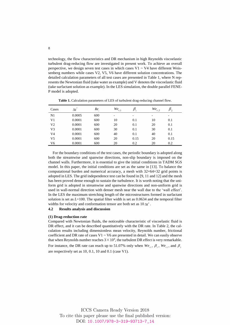
detailed calculation parameters of all test cases are presented in Table 1, where N rep-
resents the Newtonian fluid (take water as example) and V denotes the viscoelastic fluid
(take surfactant solution as example). In the LES simulation, the double parallel FENE-
P model is adopted.
Table 1. Calculation parameters of LES of turbulent drag-reducing channel flow.
Cases *
t Re
,1We
1 ,2
We
2
N1 0.0005 600 - - - -
V1 0.0001 600 10 0.1 10 0.1
V2 0.0001 600 20 0.1 20 0.1
V3 0.0001 600 30 0.1 30 0.1
V4 0.0001 600 40 0.1 40 0.1
V5 0.0001 600 20 0.15 20 0.15
V6 0.0001 600 20 0.2 20 0.2
For the boundary conditions of the test cases, the periodic boundary is adopted along
both the streamwise and spanwise directions, non-slip boundary is imposed on the
channel walls. Furthermore, it is essential to give the initial conditions in TADM SGS
model. In this paper, the initial conditions are set as the same in [13]. To balance the
computational burden and numerical accuracy, a mesh with 32×64×32 grid points is
adopted in LES. The grid independence test can be found in [9, 11 and 12] and the mesh
has been proved dense enough to sustain the turbulence. It is worth noting that the uni-
form grid is adopted in streamwise and spanwise directions and non-uniform grid is
used in wall-normal direction with denser mesh near the wall due to the ‘wall effect’.
In the LES the maximum stretching length of the microstructures formed in surfactant
solution is set as L=100. The spatial filter width is set as 0.0634 and the temporal filter
widths for velocity and conformation tensor are both set as 10 t .
4.2 Results analysis and discussion
(1) Drag-reduction rate
Compared with Newtonian fluids, the noticeable characteristic of viscoelastic fluid is
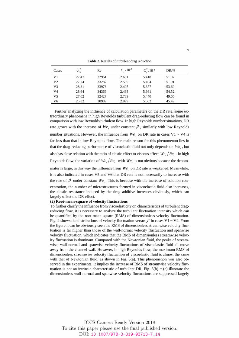
DR effect, and it can be described quantitatively with the DR rate. In Table 2, the cal-
culation results including dimensionless mean velocity, Reynolds number, frictional
coefficient and DR rate of cases V1 ~ V6 are presented in detail. We can easily observe
that when Reynolds number reaches 3×10⁴, the turbulent DR effect is very remarkable.
For instance, the DR rate can reach up to 51.07% only when 1
We
, 1
, 2
We
, and 2
are respectively set as 10, 0.1, 10 and 0.1 (case V1).
ICCS Camera Ready Version 2018To cite this paper please use the final published version:
DOI: 10.1007/978-3-319-93713-7_14
9
Table 2. Results of turbulent drag reduction
Cases +
bU
Re
fC /10-3
D
fC /10-3 DR/%
V1 27.47 32961 2.651 5.418 51.07
V2 27.74 33287 2.599 5.404 51.91
V3 28.31 33976 2.495 5.377 53.60
V4 28.64 34369 2.438 5.361 54.52
V5 27.02 32427 2.739 5.440 49.65
V6 25.82 30989 2.999 5.502 45.49
Further analyzing the influence of calculation parameters on the DR rate, some ex-
traordinary phenomena in high Reynolds turbulent drag-reducing flow can be found in
comparison with low Reynolds turbulent flow. In high Reynolds number situations, DR
rate grows with the increase of We
under constant , similarly with low Reynolds
number situations. However, the influence from We
on DR rate in cases V1 ~ V4 is
far less than that in low Reynolds flow. The main reason for this phenomenon lies in
that the drag-reducing performance of viscoelastic fluid not only depends on We
, but
also has close relation with the ratio of elastic effect to viscous effect We Re
. In high
Reynolds flow, the variation of We Re
with We
is not obvious because the denom-
inator is large, in this way the influence from We
on DR rate is weakened. Meanwhile,
it is also indicated in cases V5 and V6 that DR rate is not necessarily to increase with
the rise of under constant We
. This is because with the increase of solution con-
centration, the number of microstructures formed in viscoelastic fluid also increases,
the elastic resistance induced by the drag additive increases obviously, which can
largely offset the DR effect.
(2) Root-mean-square of velocity fluctuations
To further clarify the influence from viscoelasticity on characteristics of turbulent drag-
reducing flow, it is necessary to analyze the turbulent fluctuation intensity which can
be quantified by the root-mean-square (RMS) of dimensionless velocity fluctuation.
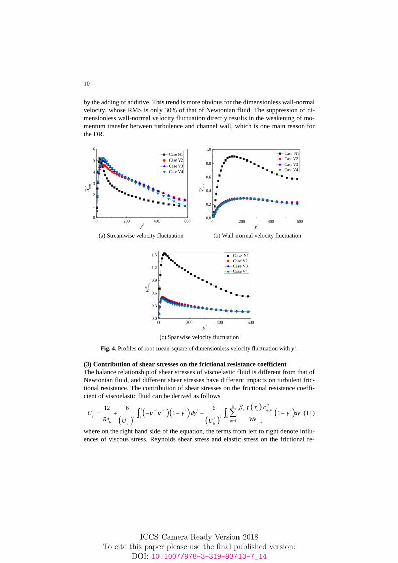
Fig. 4 shows the distributions of velocity fluctuation versus y+ in cases V1 ~ V4. From
the figure it can be obviously seen the RMS of dimensionless streamwise velocity fluc-
tuation is far higher than those of the wall-normal velocity fluctuation and spanwise
velocity fluctuation, which indicates that the RMS of dimensionless streamwise veloc-
ity fluctuation is dominant. Compared with the Newtonian fluid, the peaks of stream-
wise, wall-normal and spanwise velocity fluctuations of viscoelastic fluid all move
away from the channel wall. However, in high Reynolds flow, the maximum RMS of
dimensionless streamwise velocity fluctuation of viscoelastic fluid is almost the same
with that of Newtonian fluid, as shown in Fig. 5(a). This phenomenon was also ob-
served in the experiments, it implies the increase of RMS of streamwise velocity fluc-
tuation is not an intrinsic characteristic of turbulent DR. Fig. 5(b) ~ (c) illustrate the
dimensionless wall-normal and spanwise velocity fluctuations are suppressed largely
ICCS Camera Ready Version 2018To cite this paper please use the final published version:
DOI: 10.1007/978-3-319-93713-7_14
10
by the adding of additive. This trend is more obvious for the dimensionless wall-normal
velocity, whose RMS is only 30% of that of Newtonian fluid. The suppression of di-
mensionless wall-normal velocity fluctuation directly results in the weakening of mo-
mentum transfer between turbulence and channel wall, which is one main reason for
the DR.
0 200 400 6000
1
2
3
4
5
6
u+
'rm
s
y+
Case N1
Case V2
Case V3
Case V4
0 200 400 6000.0
0.2
0.4
0.6
0.8
1.0 Case N1
Case V2
Case V3
Case V4
v+
'rm
s
y+
(a) Streamwise velocity fluctuation (b) Wall-normal velocity fluctuation
0 200 400 6000.0
0.3
0.6
0.9
1.2
1.5 Case N1
Case V2
Case V3
Case V4
w+
'rm
s
y+
(c) Spanwise velocity fluctuation
Fig. 4. Profiles of root-mean-square of dimensionless velocity fluctuation with y+.
(3) Contribution of shear stresses on the frictional resistance coefficient
The balance relationship of shear stresses of viscoelastic fluid is different from that of
Newtonian fluid, and different shear stresses have different impacts on turbulent fric-
tional resistance. The contribution of shear stresses on the frictional resistance coeffi-
cient of viscoelastic fluid can be derived as follows
1 1' ' * * * *
2 20 0
,
1b ,b b
12 6 61 1
m
Nm xy m
f
mm
f r cC u v y dy y dy
Re WeU U
(11)
where on the right hand side of the equation, the terms from left to right denote influ-
ences of viscous stress, Reynolds shear stress and elastic stress on the frictional re-
ICCS Camera Ready Version 2018To cite this paper please use the final published version:
DOI: 10.1007/978-3-319-93713-7_14
11
sistance coefficient, which are named as viscous contribution (VC), turbulent contribu-
tion (TC) and elastic contribution (EC), respectively. Especially, elastic contribution is
equal to zero in Newtonian fluid.
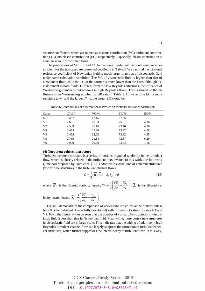
The proportions of VC, EC and TC to the overall turbulent frictional resistance co-
efficient for the test cases are presented detailedly in Table 3. We can find the frictional
resistance coefficient of Newtonian fluid is much larger than that of viscoelastic fluid
under same calculation condition. The VC of viscoelastic fluid is higher than that of
Newtonian fluid while the TC of the former is much lower than the later, although TC
is dominant in both fluids. Different from the low Reynolds situations, the influence of
Weissenberg number is not obvious in high Reynolds flows. This is similar to the in-
fluence from Weissenberg number on DR rate in Table 2. However, the EC is more
sensitive to and the larger is, the larger EC would be.
Table 3. Contributions of different shear stresses on frictional resistance coefficient.
Cases Cf/10-3 VC/% TC/% EC/%
N1 3.487 12.15 87.85 —
V1 2.651 20.33 75.61 4.06
V2 2.599 22.16 73.46 4.38
V3 2.495 21.80 73.92 4.28
V4 2.438 22.33 73.32 4.35
V5 2.739 21.14 72.57 6.29
V6 2.999 19.00 73.44 7.56
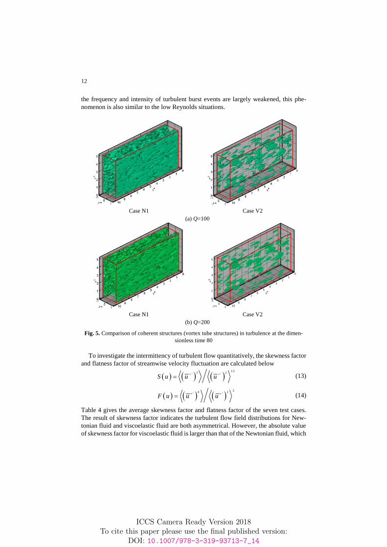
(4) Turbulent coherent structure
Turbulent coherent structure is a series of motions triggered randomly in the turbulent
flow, which is closely related to the turbulent burst events. In this work, the following
Q method proposed by Hunt et al. [16] is adopted to extract one of coherent structures
(vortex tube structure) in the turbulent channel flows
1
02
ij ij ij ijW WQ S S > (12)
where ijW is the filtered vorticity tensor, 1
=2
j iij
i j
u uW
x x
; ijS is the filtered ve-
locity-strain tensor, 1
=2
j i
ij
i j
u uS
x x
.
Figure 5 demonstrates the comparison of vortex tube structures at the dimensionless
time 80 (the turbulent flow is fully developed) with different Q values in cases N1 and
V2. From the figure, it can be seen that the number of vortex tube structures in viscoe-
lastic fluid is less than that in Newtonian fluid. Meanwhile, more vortex tube structures
in viscoelastic fluid are in large scale. This indicates that the adding of additive in high
Reynolds turbulent channel flow can largely suppress the formation of turbulent coher-
ent structures, which further suppresses the intermittency of turbulent flow. In this way,
ICCS Camera Ready Version 2018To cite this paper please use the final published version:
DOI: 10.1007/978-3-319-93713-7_14
12
the frequency and intensity of turbulent burst events are largely weakened, this phe-
nomenon is also similar to the low Reynolds situations.
Case N1 Case V2
(a) Q=100
Case N1 Case V2
(b) Q=200
Fig. 5. Comparison of coherent structures (vortex tube structures) in turbulence at the dimen-
sionless time 80
To investigate the intermittency of turbulent flow quantitatively, the skewness factor
and flatness factor of streamwise velocity fluctuation are calculated below
1.5
3 2' '
S u u u
(13)
2
4 2' '
F u u u
(14)
Table 4 gives the average skewness factor and flatness factor of the seven test cases.
The result of skewness factor indicates the turbulent flow field distributions for New-
tonian fluid and viscoelastic fluid are both asymmetrical. However, the absolute value
of skewness factor for viscoelastic fluid is larger than that of the Newtonian fluid, which
0
1
2
3
4
5
z*
01
23
45
67
89
10
x*
-10
1y*
Frame 001 27 Mar 2017 Frame 001 27 Mar 2017
ICCS Camera Ready Version 2018To cite this paper please use the final published version:
DOI: 10.1007/978-3-319-93713-7_14

13
indicates a higher asymmetry and larger deviation from Gaussian field in the viscoelas-
tic fluid. It can also be found the flatness factor of Newtonian fluid is larger than that
of viscoelastic fluid, indicating that the probability density function of streamwise ve-
locity in viscoelastic fluid is flatter than that of Newtonian fluid. Therefore, the overall
intermittency of turbulent channel flow is suppressed and the turbulent fluctuation and
burst events are obviously weakened.
Table 4. Calculation results of average skewness factor and flatness factor.
Cases Skewness factor Flatness factor
N1 0.091 5.450
V1 -0.309 4.177
V2 -0.368 4.212
V3 -0.390 4.562
V4 -0.327 4.325
V5 -0.293 4.250
V6 -0.262 3.953
Gaussian field 0 3
5 Conclusions
In this paper, we apply the LES approach to investigate turbulent DR mechanism in
viscoelastic turbulent drag-reducing flow with high Reynolds number based on an N-
parallel FENE-P model and MICT SGS model. The main conclusions of this work are
as follows
(1) There is a notable difference of flow characteristics between high Reynolds and
low Reynolds turbulent drag-reducing flows. For instance, the RMS peak value of di-
mensionless streamwise velocity fluctuation in high Reynolds turbulent flow is not ob-
viously strengthened as in low Reynolds turbulent flow.
(2) The influence of calculation parameters on frictional resistance coefficients in
high Reynolds turbulent drag-reducing flow also differs from that in low Reynolds sit-
uations. For example, the effect of Weissenberg number exerted to turbulent flow is not
obvious while influence of on elastic contribution is more remarkable.
(3) The number of vortex tube structures in high Reynolds turbulent drag-reducing
flow with viscoelastic fluid is much less than that in Newtonian turbulent flow. Com-
pared with the Newtonian fluid, the turbulent flow field of viscoelastic fluid is featured
by higher asymmetry and more large-scale motions with low frequency.
Acknowledgements
The study is supported by National Natural Science Foundation of China (No.
51636006), project of Construction of Innovative Teams and Teacher Career Develop-
ment for Universities and Colleges under Beijing Municipality (No. IDHT20170507)
and the Program of Great Wall Scholar(CIT&TCD20180313).
ICCS Camera Ready Version 2018To cite this paper please use the final published version:
DOI: 10.1007/978-3-319-93713-7_14
14
References
1. Savins J. G.: Drag reductions characteristics of solutions of macromolecules in turbulent
pipe flow. Society of Petroleum Engineers Journal 4(4), 203–214 (1964).
2. Renardy M., Renardy Y.: Linear stability of plane couette flow of an upper convected max-
well fluid. Journal of Non-Newtonian Fluid Mechanics 22(1), 23–33 (1986).
3. Oldroyd J. G.: On the formulation of rheological equations of state. Proceedings of the Royal
Society A: Mathematical, Physical & Engineering Sciences, 200(1063): 523–541 (1950).
4. Oliveria P. J.: Alternative derivation of differential constitutive equations of the Oldroyd-B
type. Journal of Non-Newtonian Fluid Mechanics 160(1), 40–46 (2009).
5. Giesekus H.: A simple constitutive equation for polymer fluids based on the concept of de-
formation-dependent tensorial mobility. Journal of Non-Newtonian Fluid Mechanics 11(1),
69–109 (1982).
6. Bird R. B., Doston P. J., Johnson N. L.: Polymer solution rheology based on a finitely ex-
tensible bead-spring chain model. Journal of Non-Newtonian Fluid Mechanics 7(2-3), 213–
235 (1980).
7. Wei J. J., Yao Z. Q.: Rheological characteristics of drag-reducing surfactant solution. Jour-
nal of Chemical Industry and Engineering (In Chinese) 58(2), 0335–0340 (2007).
8. Li J. F., Yu B., Sun S. Y., Sun D. L.: Study on an N-parallel FENE-P constitutive model
based on multiple relaxation times for viscoelastic fluid. In: Shi Y., Fu H. H.,
Krzhizhanovskaya V. V., Lees M. H., Dongarra J. J., Sloot P. M. A. (eds.) International
Conference on Computational Science (ICCS-2018), Springer, Heidelberg (2018). (Ac-
cepted)
9. Thais L., Tejada-Martínez A. E., Gatski T. B., Mompean G.: Temporal large eddy simula-
tions of turbulent viscoelastic drag reduction flows. Physics of Fluids 22(1), 013103 (2010).
10. Wang L., Cai W. H., Li F. C.: Large-eddy simulations of a forced homogeneous isotropic
turbulence with polymer additives. Chinese Physics B 23(3), 034701 (2014).
11. Li F. C., Wang L., Cai W. H.: New subgrid-scale model based on coherent structures and
temporal approximate deconvolution, particularly for LES of turbulent drag-reducing flows
of viscoelastic fluids. China Physics B 24(7), 074701 (2015).
12. Kobayashi H.: The subgrid-scale models based on coherent structures for rotating homoge-
neous turbulence and turbulent channel flow. Physics of Fluids 17(4), 045104 (2005).
13. Li J. F., Yu B., Wang L., Li F. C., Hou L.: A mixed subgrid-scale model based on ICSM
and TADM for LES of surfactant-induced drag-reduction in turbulent channel flow. Applied
Thermal Engineering 115, 1322–1329 (2017).
14. Li J. F., Yu B., Zhao Y., Wang Y., Li W.: Flux conservation principle on construction of
residual restriction operators for multigrid method. International Communications in Heat
and Mass Transfer 54, 60-66 (2014).
15. Li F. C., Yu B., Wei J. J., Kawaguchi Y.: Turbulent drag reduction by surfactant additives.
Higher Education Press, Beijing (2012).
16. Hunt J. C. R., Wray A., Moin P.: Eddies, stream and convergence zones in turbulence flows.
Studying Turbulence Using Numerical Simulation Databases 1, 193–208 (1988).
ICCS Camera Ready Version 2018To cite this paper please use the final published version:
DOI: 10.1007/978-3-319-93713-7_14
Top Related