


Languages
Pages
Legal


Springer Undergraduate Mathematics Series
From Natural Numbers to Quaternions
Jürg KramerAnna-Maria von Pippich

Springer Undergraduate Mathematics Series
Advisory Board
M. A. J. Chaplain, University of St. AndrewsA. MacIntyre, Queen Mary University of LondonS. Scott, King’s College LondonN. Snashall, University of LeicesterE. Süli, University of OxfordM. R. Tehranchi, University of CambridgeJ. F. Toland, University of Cambridge

More information about this series at http://www.springer.com/series/3423

Jürg Kramer • Anna-Maria von Pippich
From Natural Numbersto Quaternions
123

Jürg KramerDepartment of MathematicsHumboldt-Universität zu BerlinGermany
Anna-Maria von PippichDepartment of MathematicsTechnische Universität DarmstadtGermany
Translation from the German language edition: Von den natürlichen Zahlen zu denQuaternionen by Jürg Kramer and Anna-Maria von Pippich, © Springer Spektrum 2013. AllRights Reserved.
ISSN 1615-2085 ISSN 2197-4144 (electronic)Springer Undergraduate Mathematics SeriesISBN 978-3-319-69427-6 ISBN 978-3-319-69429-0 (eBook)https://doi.org/10.1007/978-3-319-69429-0
Library of Congress Control Number: 2017958024
Mathematics Subject Classification (2010): 08–01, 11–01, 12–01, 20–01
© Springer International Publishing AG 2017This work is subject to copyright. All rights are reserved by the Publisher, whether the whole or partof the material is concerned, specifically the rights of translation, reprinting, reuse of illustrations,recitation, broadcasting, reproduction on microfilms or in any other physical way, and transmissionor information storage and retrieval, electronic adaptation, computer software, or by similar or dissimilarmethodology now known or hereafter developed.The use of general descriptive names, registered names, trademarks, service marks, etc. in thispublication does not imply, even in the absence of a specific statement, that such names are exempt fromthe relevant protective laws and regulations and therefore free for general use.The publisher, the authors and the editors are safe to assume that the advice and information in thisbook are believed to be true and accurate at the date of publication. Neither the publisher nor theauthors or the editors give a warranty, express or implied, with respect to the material contained herein orfor any errors or omissions that may have been made. The publisher remains neutral with regard tojurisdictional claims in published maps and institutional affiliations.
Printed on acid-free paper
This Springer imprint is published by Springer NatureThe registered company is Springer International Publishing AGThe registered company address is: Gewerbestrasse 11, 6330 Cham, Switzerland

Preface to the English Edition
This book on the construction of number systems first appeared in 2013 in aGerman edition with the same title. It can be seen from the following prefaceto that edition that the goal of this book is to present a basic and compre-hensive construction of number systems, beginning with the natural num-bers and ending with Hamilton’s quaternions, while providing relevant al-gebraic knowledge along the way. As a supplement to the German edition,an appendix has been added to each chapter in this English edition, whichin contrast to the rigorous style of the rest of the book, presents in the morecasual form of a survey some related aspects of the material of the chapter,including some recent developments.
We would like to offer our most heartfelt thanks to the translator, DavidKramer, for his competent work, which has contributed significantly to thisEnglish version and in many places led to a more felicitous presentation ofthe material.
We hope that this book will help students and teachers of mathematicsas well as all those with an interest in the subject to fill in any gaps in theirmathematical education related to the construction of number systems andthat the appendices will inspire some readers to pursue further mathemati-cal studies.
Berlin, September 2017 Jürg KramerAnna-Maria von Pippich
Preface to the German Edition
The main topic of this book is an elementary introduction to the construc-tion of the number systems encountered by mathematics students in theirfirst semesters of study. Beginning with the natural numbers, we succes-sively construct, along with the requisite algebraic machinery, all the num-ber fields containing the natural numbers, including the real numbers, com-plex numbers, and Hamiltonian quaternions. Our experience has shown usthat time is frequently lacking in introductory mathematics courses for awell-founded construction of number systems; this book represents a con-tribution toward filling that gap.
The construction of number systems also represents an important compo-nent in the professional education of mathematics teachers. For this reason,this book offers a self-contained and compact construction of the numbersystems that are of relevance to different grade levels from a mathematicalperspective with a view toward aspects of pedagogical content knowledge.
This book arose from a course in elementary abstract algebra and numbertheory given a number of times at the Humboldt University of Berlin. Partsof the first-named author’s book Zahlen für Einsteiger: Elemente der Algebraund Zahlentheorie (Vieweg Verlag, Wiesbaden, 2008) have been revised andexpanded for inclusion in this newly conceived book on the construction ofnumber systems. Numerous exercises with extensive solutions facilitate thereader’s engagement with the subject.
The completion of this book would not have been possible without thecontributions of many individuals. Here we wish to thank first of all ChristaDobers and Matthias Fischmann for typing the first parts of the manuscript.In addition, we wish to thank all the students whose written course notescontributed to the text. We also wish to thank our colleagues, in particu-lar Andreas Filler and Wolfgang Schulz, for their numerous suggestions forimproving early versions of the manuscript. A special word of thanks goesto Olaf Teschke for his work on creating the exercises, and we also thankBarbara Jung and André Henning for their work on writing up solutionsto the exercises. Finally, we offer hearty thanks to Christoph Eyrich for hisexpert support in designing the layout of the book and to Ulrike Schmickler-Hirzebruch for her encouragement and support on behalf of the publisher,Springer Spektrum.
Berlin, February 2013 Jürg KramerAnna-Maria von Pippich
Table of Contents
Preface to the English Edition v
Preface to the German Edition vii
Introduction 1
I The Natural Numbers 91. The Peano Axioms . . . . . . . . . . . . . . . . . . . . . . . . . . . . . . . . . . . . . . . . . . . . 92. Divisibility and Prime Numbers . . . . . . . . . . . . . . . . . . . . . . . . . . . . . . . . 153. The Fundamental Theorem of Arithmetic . . . . . . . . . . . . . . . . . . . . . . . 224. Greatest Common Divisor, Least Common Multiple . . . . . . . . . . . . . 255. Division with Remainder . . . . . . . . . . . . . . . . . . . . . . . . . . . . . . . . . . . . . . 29A. Prime Numbers: Facts and Conjectures . . . . . . . . . . . . . . . . . . . . . . . . . 32
II The Integers 451. Semigroups and Monoids . . . . . . . . . . . . . . . . . . . . . . . . . . . . . . . . . . . . . . 452. Groups and Subgroups . . . . . . . . . . . . . . . . . . . . . . . . . . . . . . . . . . . . . . . . 483. Group Homomorphisms . . . . . . . . . . . . . . . . . . . . . . . . . . . . . . . . . . . . . . 544. Cosets and Normal Subgroups . . . . . . . . . . . . . . . . . . . . . . . . . . . . . . . . . 575. Quotient Groups and the Homomorphism Theorem . . . . . . . . . . . . . 636. Construction of Groups from Regular Semigroups . . . . . . . . . . . . . . . 687. The Integers . . . . . . . . . . . . . . . . . . . . . . . . . . . . . . . . . . . . . . . . . . . . . . . . . . 73B. RSA Encryption: An Application of Number Theory . . . . . . . . . . . . . 77
III The Rational Numbers 931. The Integers and Divisibility Theory . . . . . . . . . . . . . . . . . . . . . . . . . . . . 932. Rings and Subrings . . . . . . . . . . . . . . . . . . . . . . . . . . . . . . . . . . . . . . . . . . . 973. Ring Homomorphisms, Ideals, and Quotient Rings . . . . . . . . . . . . . . 1024. Fields and Skew Fields . . . . . . . . . . . . . . . . . . . . . . . . . . . . . . . . . . . . . . . . 1105. Construction of Fields from Integral Domains . . . . . . . . . . . . . . . . . . . 1126. The Rational Numbers . . . . . . . . . . . . . . . . . . . . . . . . . . . . . . . . . . . . . . . . 1177. Unique Factorization Domains, Principal Ideal Domains, and
Euclidean Domains . . . . . . . . . . . . . . . . . . . . . . . . . . . . . . . . . . . . . . . . . . . 119C. Rational Solutions of Equations: A First Glimpse . . . . . . . . . . . . . . . . 129
IV The Real Numbers 1411. Decimal Representation of Rational Numbers . . . . . . . . . . . . . . . . . . . 1412. Construction of the Real Numbers . . . . . . . . . . . . . . . . . . . . . . . . . . . . . . 1453. The Decimal Expansion of a Real Number . . . . . . . . . . . . . . . . . . . . . . 155

x Table of Contents
4. Equivalent Characterizations of Completeness . . . . . . . . . . . . . . . . . . 1595. The Real Numbers and the Real Number Line . . . . . . . . . . . . . . . . . . . 1646. The Axiomatic Point of View . . . . . . . . . . . . . . . . . . . . . . . . . . . . . . . . . . . 168D. The p-adic Numbers: Another Completion ofQ . . . . . . . . . . . . . . . . . 171
V The Complex Numbers 1831. The Complex Numbers as a Real Vector Space . . . . . . . . . . . . . . . . . . . 1832. Complex Numbers of Modulus 1 and the Special Orthogonal
Group . . . . . . . . . . . . . . . . . . . . . . . . . . . . . . . . . . . . . . . . . . . . . . . . . . . . . . . . 1873. The Fundamental Theorem of Algebra . . . . . . . . . . . . . . . . . . . . . . . . . . 1914. Algebraic and Transcendental Numbers . . . . . . . . . . . . . . . . . . . . . . . . 1935. The Transcendence of e . . . . . . . . . . . . . . . . . . . . . . . . . . . . . . . . . . . . . . . . 197E. Zeros of Polynomials: The Search for Solution Formulas . . . . . . . . . . 204
VI Hamilton’s Quaternions 2191. Hamilton’s Quaternions as a Real Vector Space . . . . . . . . . . . . . . . . . . 2192. Quaternions of Modulus 1 and the Special Unitary Group . . . . . . . . 2233. Quaternions of Modulus 1 and the Special Orthogonal Group . . . . 227F. Extensions of Number Systems: What Comes after the
Quaternions? . . . . . . . . . . . . . . . . . . . . . . . . . . . . . . . . . . . . . . . . . . . . . . . . . 231
Solutions to Exercises 247
Selected Literature 279
Index 283

Introduction
The Development of the Integers and Algebra
One of mankind’s earliest intellectual occupations was counting. The devel-opment of the concepts of numbers and the representation of numbers hastherefore assumed a place of importance in the history of every civilization.The enormous effectiveness of our decimal system of numerical represen-tation is the culmination of centuries—indeed millennia—of earlier effortsthat together represent a powerful cultural attainment.
The idea of counting objects, that is, of bringing a set of equivalent objectsinto a one-to-one correspondence with a fixed set of numbers, represents asignificant intellectual process of abstraction.
In more advanced cultures, systems of symbolic notation for these num-bers—some more effective than others—were developed. We mention par-ticularly the cuneiform writing of the Babylonians, Egyptian hieroglyphics,Roman numerals, and the system of numerals developed in India. It wasonly in the thirteenth and fourteenth centuries that the Indian positionaldecimal system finally made its way via the Islamic world to Western Eu-rope, which to this day uses “Arabic” numerals.
The development of number systems goes relatively closely hand in handwith the development of methods of calculation. In this regard, the Babylo-nian and Indian number systems, for example, were far superior to those ofthe Egyptians and Romans. Nevertheless, until late in the fifteenth century,in both the ancient civilizations and Western Europe, numerical calculationwas the province of a small group of specialists known as arithmeticians. Itwas not until the publication in the fifteenth century of Adam Ries’s bookson calculation, which were based on the book Liber Abaci of Leonardo ofPisa, known as Fibonacci, that the usual methods of calculation that we usetoday became accessible to the “common people.” The diffusion of calcula-tional techniques is linked to a systemization of arithmetic in the academicworld, which then led to the development of algebra. At first, algebra wasviewed primarily as a practical tool, but it gradually took on a life of its ownand eventually developed into the independent discipline that we know to-day. Algebra will therefore play a significant role in every rigorous scientifi-cally based construction of number systems.

2 Introduction
A First Look at Number Systems
We all recall from our schooldays how we first learned about the numbers1, 2, 3, . . . , then the square roots of such numbers, for example
√2, and some-
what later became acquainted with the number π, associated with the cir-cumference of a circle, and perhaps Euler’s constant e. On our first encounterwith these numbers, we had no idea that a powerful intellectual constructhad to be developed before a number system could be created that couldcontain all these numbers and make possible a “sensible” way of calculatingwith them, namely the system of real numbers. The creation of this numbersystem represents an outstanding achievement of the human intellect, anda fundamental objective of this book is to acquaint students with the con-struction of the real numbers so that they may become familiar with the finestructure of these objects.
It is astounding that the set of real numbers, which we denote by R,can be developed essentially from the single number 1 (one). Let us sketchbriefly how this is done, for a thoroughgoing working out of this process isthe main purpose of this book. We begin by identifying the number 1 withan object, and we then bring along another object of the same kind, so thatwe now have two objects and thereby have acquired the number 2. We mayformalize this process by writing 2 = 1 + 1. Continuing in this manner, weobtain in sequence the numbers
3 = 2 + 1 = 1 + 1 + 1,4 = 3 + 1 = 1 + 1 + 1 + 1,· · ·
that is, the set of natural numbers N except for the number 0 (zero), whichwe shall obtain momentarily, and append to the set of natural numbers. Onemight say that the number 1 generates additively every natural number.That is, the number 1 is, from an additive point of view, the atom from whichevery natural number is built.
We may picture the natural numbers 1, 2, 3, . . . as sitting equally spacedlike pearls on a necklace beginning at the left with 1 and continuing sequen-tially off to the right. We might also represent these numbers geometrically,to which end we choose a unit length and mark it off on a horizontal line Lby beginning at a point P and moving to the right. We denote by the symbol1 the point on the line thereby constructed. Continuing, we obtain a secondpoint, which we denote by 2, and so on:
L�
P
�
3
�
2
�
1For no reason other than symmetry we might wish to carry out a similarprocess by moving to the left. Of course, the new points that we thereby
3
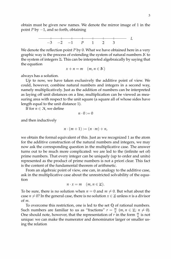
obtain must be given new names. We denote the mirror image of 1 in thepoint P by −1, and so forth, obtaining
L�
P
�
3
�
2
�
1
�
−1
�
−2
�
−3
We denote the reflection point P by 0. What we have obtained here in a verygraphic way is the process of extending the system of natural numbersN tothe system of integers Z. This can be interpreted algebraically by saying thatthe equation
x + n = m (m, n ∈N)
always has a solution.Up to now, we have taken exclusively the additive point of view. We
could, however, combine natural numbers and integers in a second way,namely multiplicatively. Just as the addition of numbers can be interpretedas laying off unit distances on a line, multiplication can be viewed as mea-suring area with respect to the unit square (a square all of whose sides havelength equal to the unit distance 1).
If for n ∈N, we definen · 0 := 0
and then inductively
n · (m + 1) := (n ·m) + n,
we obtain the formal equivalent of this. Just as we recognized 1 as the atomfor the additive construction of the natural numbers and integers, we maynow ask the corresponding question in the multiplicative case. The answerturns out to be much more complicated: we are led to the (infinite set of)prime numbers. That every integer can be uniquely (up to order and units)represented as the product of prime numbers is not a priori clear. This factis the content of the fundamental theorem of arithmetic.
From an algebraic point of view, one can, in analogy to the additive case,ask in the multiplicative case about the unrestricted solvability of the equa-tion
n · x = m (m, n ∈ Z).To be sure, there is no solution when n = 0 and m 6= 0. But what about thecase n 6= 0? In the general case, there is no solution x ∈Z unless n is a divisorof m.
To overcome this restriction, one is led to the set Q of rational numbers.Such numbers are familiar to us as “fractions” r = m
n (m, n ∈ Z; n 6= 0).One should note, however, that the representation of r in the form m
n is notunique: we can make the numerator and denominator larger or smaller us-ing the relation

4 Introduction
r =mn=
m′
n′⇐⇒ m · n′ = n ·m′.
It is therefore essential in understanding the setQ that we imagine a rationalnumber as a class of pairs of integers. At this point, there are several ways inwhich we might motivate a further enlargement of our number system. Forexample, we could follow the ancient Greeks and use the fundamental the-orem of arithmetic to demonstrate that the length of the diagonal of the unitsquare, that is, the “number”
√2, is not rational, which would then require
an enlargement of the number system Q. Another possibility is the follow-ing: using the geometric representation of the integers as points on a line tocreate an extension to the rational numbers using properties of similar tri-angles, we obtain these new rational numbers as additional points that are“densely packed” on the line. The question now arises whether these newlyobtained points constitute the entire number line, that is, whether the ratio-nal numbers fill up the number line without leaving any gaps. As is wellknown, there are such gaps, and we are then motivated to attempt to fillthem in. Once again, one is led to an extension of the set of rational numbersQ and thereby to the construction of the real numbersR. This nontrivial pro-cess of completion of the rational numbers has wide-ranging consequences,since it lays the foundation for calculus and thereby makes it possible, forexample, to handle differential equations, which describe many processes inthe real world.
Detailed Outline of This Book
There are various aspects of the natural numbers that can provide us an ori-entation. One relies primarily on the cardinal aspect (counting aspect) and theordinal aspect (ordering aspect) of the natural numbers. The cardinal aspectrests on the equivalence classes of sets of equal size, while the ordinal aspectis based on the assumption that the set of natural numbers has a beginningpoint, that every natural number has exactly one successor number, and thatdistinct natural numbers have distinct successors. In the framework of ouraxiomatic approach, we turn to the ordinal aspect and establish the natu-ral numbers at the beginning of the first chapter with the help of Peano’saxioms. Using the fifth Peano axiom, namely the axiom of mathematicalinduction, we define addition and multiplication of the natural numbersand introduce the usual arithmetic operations. In the second part of the firstchapter, we develop the concept of divisibility of natural numbers; the mainresult of this part is the proof of the fundamental theorem of arithmetic. Thefirst chapter ends with a section on division with remainder, in which thedecimal representation of numbers plays an important role.
The operations of addition and multiplication of natural numbers devel-oped in the first chapter are abstracted in the second chapter, leading to the
5
definitions of semigroups and monoids. These notions begin our construc-tion of number systems through the necessary algebraic concepts that wedevelop in the second and third chapters. In the second chapter, we concen-trate above all on an elementary presentation of group theory, introducinggroups, subgroups, normal subgroups, group homomorphisms, cosets, andquotient groups. These theoretical considerations lead to the fact that regu-lar abelian semigroups can be extended essentially uniquely to groups. Thisyields in particular the mathematically based extension of the additive semi-group (N, +) of natural numbers to the additive group (Z, +) of integers.
The extension of the multiplication of natural numbers to the newly con-structed domain of the integers leads to the algebraic concept of a ring. Thestudy of the fundamental aspects of ring theory is the subject of the thirdchapter. In this connection, we study rings, subrings, ideals, ring homomor-phisms, and quotient rings. We discover the special classes of rings knownas integral domains and fields, which again play an important role in theconstruction of number systems. In fields, for example, division of two el-ements can be carried out in every case, provided the denominator is notzero. We shall see that every integral domain can be enlarged to a field. Sincethe ring (Z,+, ·) will turn out to be an integral domain, we will be able toenlarge it to the field (Q,+, ·) of rational numbers. The third chapter closeswith a discussion of special rings motivated by an algebraic systemizationof the concept of divisibility.
To begin the fourth chapter, we apply the decimal representation of inte-gers to the set of rational numbers that we constructed in the third chapter.We thereby obtain the decimal fraction development of rational numbers. Itturns out that such a representation of a rational number either terminatesor is periodic. This raises the question whether there exists an extension ofthe rational numbers that contains all “numbers” that can be representedby an arbitrary decimal expansion. As we shall see, this is the set of realnumbers, but we have far to go before we can carry out that construction:with the help of the quotient ring of rational Cauchy sequences modulo theideal of rational null sequences, we first construct a field that contains Q.We determine that this field is complete, that is, that every Cauchy sequencewith elements in this field has a limit in this field. From this, we achieve theinsight that this abstractly constructed field can be identified with the set ofnumbers represented by infinite decimals, which leads to the field R of realnumbers. In the last part of the chapter, we consider alternative characteri-zations of the completeness of R, such as the existence of the supremum ofevery subset of R that is bounded from above. Another important point atthe end of this chapter is the identification ofRwith the number line, whichbecomes possible only after the axioms of classical Euclidean geometry areextended by a further axiom that postulates that the number line has, so tospeak, no holes.
The fifth chapter begins with the question of a further extension of the setof real numbers: given that the integers and rational numbers were created
6 Introduction
with the goal of being able to solve every linear equation of the form
a · x + b = c (a, b, c ∈N; a 6= 0),
the question naturally arises concerning the solvability of equations of higherdegree, for example those of degree 2. With quadratic extensions it becomesclear that the solution of quadratic equations implies the existence of squareroots. It turns out that real square roots exist for every positive real number.In contrast, no negative real number has a real square root. By postulatingthat the number −1 has the imaginary unit i as a square root, we are led tothe fieldC of complex numbers. Having constructedC, we soon come to theconclusion that extraction of square roots can be carried out without restric-tion in the complex numbers. That in fact, every polynomial equation withcomplex coefficients has complex roots is the content of the fundamentaltheorem of algebra, for which we give an elementary proof. In the secondpart of the chapter we investigate the fine structure of the real (and com-plex) numbers. This leads us to the distinction between algebraic and tran-scendental numbers. Although transcendental numbers seem to be a priorimore difficult to deal with, their characterization shows that they are par-ticularly well approximated by rational numbers. The chapter closes with aproof of the transcendence of Euler’s number e = 2.71828 . . . .
Our goal in the final sixth chapter is to search for fields that extend thefield of complex numbers C to an even more encompassing field. Since wecan view C as a two-dimensional real vector space, it makes sense to be-gin by looking for a field that arises from a three-dimensional real vectorspace. It turns out, however, that no such field exists. If we then look for afield that can be obtained from a four-dimensional real vector space, we dis-cover that such a field exists, provided that we abandon the requirement ofcommutativity of multiplication. In this way, we are led to the constructionof the skew field of Hamiltonian quaternions, which brings to a close ourinvestigation of number systems.
Chapter Appendices for the Interested Reader
As mentioned in the preface, each of the six chapters in the English editionon the construction of number systems has been supplemented with an ap-pendix. These appendices have been designed for the reader who wishesto learn about some of the further developments to which the number sys-tem presented in the corresponding chapter has given rise, both historicallyand with respect to very recent results. In contrast to the systematic devel-opment of the mathematical machinery necessary for constructing numbersystems, we have adopted in the appendices a less rigorous style. This al-lows the appendices to remain largely independent of the remainder of thebook, and in particular, they should provide the student some first insights

7
into questions that are topics of current research. The choice of topics largelyrepresents the authors’ personal mathematical taste.
The appendix to the first chapter deals with interesting developments onthe subject of prime numbers, including work on conjectures that remain un-resolved to this day. The appendix to the second chapter provides an intro-duction to working with congruences, which are particularly useful in cryp-tographic applications. Building on that knowledge, we introduce the RSAencryption procedure and discuss some of its strengths and weaknesses. Inthe appendix to the third chapter we investigate the search for rational solu-tions of polynomial equations in several variables (with integer coefficients),the most famous example being the Fermat equation Xd + Yd = Zd, whichfor exponent d > 2 has only the trivial solution. In the fourth chapter, af-ter we have obtained the real numbers by completing the rational numberswith respect to the (archimedean) absolute value, we introduce in the ap-pendix the so-called p-adic completion, which leads to the p-adic numbersQp, which in turn are helpful in finding rational solutions to polynomialequations in the context of the local–global principle. Following the con-struction of the complex numbers in the fifth chapter, we turn naturally tothe question of the representation in terms of radicals of the zeros of a poly-nomial in a single variable (with complex coefficients), which turns out tobe impossible in general once the degree of the polynomial exceeds four.This leads directly to Galois theory and the current topic of so-called Galoisrepresentations. In the appendix to the last chapter, we conclude our bookby asking whether there can exist a number system that extends Hamilton’squaternions. It turns out that if we are willing to give up associativity of mul-tiplication, there is precisely one additional extension, Cayley’s octonions,which rounds out the subject of this book in a most satisfying way.
Prerequisites
A first prerequisite for the study of this book is an acquaintance with naiveset theory. We assume that the interested reader is familiar with the notionsof set, membership, and containment, as well as the operations of set in-tersection, union, and difference. Furthermore, we assume familiarity withmappings between sets and the notions of injectivity, surjectivity, and bijec-tivity of mappings. It is only in the fifth and sixth chapters that we invokein certain places the theory of finite-dimensional vector spaces, and we alsomake use of elements of the calculus of functions of a single real variable.
Final Remarks
Many interesting topics and mathematical pearls from the theories of ele-mentary number theory and abstract algebra are not mentioned in this book.

8 Introduction
We have focused primarily on the construction of number systems and theirrequisite algebraic apparatus. It is our hope that through the lens of algebra,the reader will obtain new insights into the structure of the number systemsstudied earlier in school, and in addition, will learn with the help of familiarnumbers to value the abstract and fruitful methods of algebra in the spiritof the fifth-century Greek philosopher Proclus, who wrote, “Wherever thereis number, there is beauty.”

I The Natural Numbers
1. The Peano Axioms
We begin our study of elementary number theory with a discussion of theset of natural numbers. According to Leopold Kronecker, the set of naturalnumbers {0,1,2, . . .} together with the familiar operations of addition andmultiplication may be considered as having been created by God. We shallnot go any further into metaphysics regarding the natural numbers. Instead,we are going to take an axiomatic approach to constructing sets of numbers,and we shall begin by defining the natural numbers with the help of theaxioms proposed by Giuseppe Peano.
Definition 1.1 (Peano axioms). The set N of natural numbers is character-ized by the following axioms:(i) The setN is nonempty. It contains a distinguished element 0 ∈N.(ii) For every n ∈ N, there exists a uniquely defined element n∗ ∈ N with
n∗ 6= n. The element n∗ is called the (immediate) successor of n, and n iscalled the (immediate) predecessor of n∗.
(iii) There is no element n∈Nwhose successor n∗ satisfies the relation n∗ =0. That is, the element 0 has no predecessor and is therefore consideredthe first element.
(iv) If two natural numbers n1,n2 satisfy the equality n∗1 = n∗2 , then it fol-lows that n1 = n2. That is, the successor mapping is an injection fromN toN.
(v) Principle of mathematical induction: If T is a subset ofNwith the propertythat 0∈ T (basis of the induction), and if it follows from the assumptiont ∈ T (induction hypothesis) that t∗ ∈ T as well (induction step), thenwe must have T =N.
Remark 1.2. Note that the successor of a natural number n is the immediatesuccessor n∗. By a successor of a natural number n we mean any elementof the set {n∗,n∗∗,n∗∗∗, . . .}; we will also call these numbers respectively thefirst successor, second successor, third successor, etc., of n. Similar nomen-clature holds for predecessors.
Remark 1.3. Using Definition 1.1 repeatedly, we may introduce the follow-ing familiar notation:
1 := 0∗, 2 := 1∗ = 0∗∗, 3 := 2∗ = 1∗∗ = 0∗∗∗, . . . ,
© Springer International Publishing AG 2017J. Kramer and A.-M. von Pippich, From Natural Numbers to Quaternions, Springer Undergraduate Mathematics Series, https://doi.org/10.1007/978-3-319-69429-0_1

10 I The Natural Numbers
where the multiple asterisks denote multiple applications of taking the suc-cessor. The setN of natural numbers can now be written in the familiar form
N= {0,1,2,3, . . .}.
Axiom (v) of Definition 1.1 forms the basis of constructing what are calledproofs by induction: if one wishes to prove that every natural number pos-sesses a certain property, then one may do so by first proving that the num-ber 0 possesses the given property (basis of the induction), then showingthat on the assumption that the natural number n (n ∈N arbitrary but fixed)has the property (induction hypothesis), it follows that the successor n∗ hasthe property. By Axiom (v), it follows that the property holds for all n ∈N.
We would like to note here that the principle of mathematical inductioncan be formulated in the following modified form: if T is a subset of N con-taining n0 (basis of induction) and if t ∈ T (induction hypothesis) impliest∗ ∈ T (induction step), then we must have T ⊇ {n0, n∗0 , . . .}. With induc-tion proofs of this type, it is possible to prove properties that do not holdnecessarily for all the natural numbers, but only for n0 and its successors.
Remark 1.4. One could justifiably ask whether the set of natural numbersas defined actually exists, whether there exists a model of the Peano axioms.This question can be answered in the affirmative with the help of set theory.Likewise, one can show that the natural numbers are uniquely determined,that is, that all models of the Peano axioms are equivalent (more precisely,isomorphic) to each other. We refer the reader to the vast literature on settheory.
We now define the operations of addition and multiplication of naturalnumbers.
Definition 1.5. Addition and multiplication of natural numbers m and n aredefined inductively as follows:
Addition: n + 0 := n, n + m∗ := (n + m)∗, (1)Multiplication: n · 0 := 0, n ·m∗ := (n ·m) + n. (2)
Remark 1.6. Definition 1.5 indeed constitutes a valid definition of additionand multiplication on the set of natural numbers. If one wishes, for example,to add the natural number n to the natural number m, the sum n + m isdetermined by (1) as follows: we write m in the form m = 0∗···∗ (with masterisks; that is, m is the mth successor of 0); from n + 0 = n by definition,we may deduce

1. The Peano Axioms 11
n + 1 = n + 0∗ = (n + 0)∗ = n∗,n + 2 = n + 0∗∗ = (n + 0∗)∗ = (n + 1)∗ = n∗∗,
· · ·n + m = n + 0∗···∗ = n∗···∗ (m times);
that is, the sum n + m is the mth successor of n.Similarly, the product n ·m of n,m ∈N is defined by (2). We note here that
we will frequently omit the dot symbolizing multiplication and write mninstead of m · n.
We shall now use Peano’s axioms to prove that the usual laws of additionand multiplication hold under our definition of those two operations.
Lemma 1.7. The following laws hold for arbitrary natural numbers n,m, p:Associative law:
n + (m + p) = (n + m) + p,n · (m · p) = (n ·m) · p.
Commutative law:
n + m = m + n,n ·m = m · n.
Distributive law:
(n + m) · p = (n · p) + (m · p),p · (n + m) = (p · n) + (p ·m).
Proof. We shall present a proof for the commutative law of addition. Theother proofs are similar. We shall use a double induction argument, that is,an induction on m, and embedded within that induction, an induction on n.
(i) We take m = 0 as the basis of the induction: We must show that
n + 0 = 0 + n
for all n ∈N. Since by (1), we have n + 0 = n, we must show that 0 + n = n;we do this by induction on n. For n = 0, the assertion is true. Given theinduction hypothesis that 0 + n = n for an arbitrary n ∈ N, we must showthat 0 + n∗ = n∗. Using (1) and the induction hypothesis, we see easily that
0 + n∗ = (0 + n)∗ = n∗.
This completes the induction on n and also the basis of the induction form = 0.
(ii) We now make the induction hypothesis that for m ∈N, the equality

12 I The Natural Numbers
n + m = m + n
holds for all n ∈ N. On this assumption, we now assert that we also musthave
n + m∗ = m∗ + n
for all n ∈ N. Before we prove this, we show first that m∗ + n = (m + n)∗
for all n ∈N, again using induction on n. For n = 0, the assertion follows atonce from (1). With the induction hypothesis m∗ + n = (m + n)∗, it sufficesto show that we also have m∗ + n∗ = (m + n∗)∗. This can be seen at oncefrom using (1) twice and the induction hypothesis, namely
m∗ + n∗ = (m∗ + n)∗ =((m + n)∗
)∗= (m + n∗)∗.
This allows us to complete the induction on m. Namely, using (1), the induc-tion hypothesis, and the equality that we just proved, we have
n + m∗ = (n + m)∗ = (m + n)∗ = m∗ + n.
This completes the proof of the fact that addition of natural numbers is com-mutative. ut
Exercise 1.8. Prove the remaining laws of addition and multiplication fromLemma 1.7.
Remark 1.9. In connection with the distributive law, we note that the opera-tion of multiplication takes precedence over that of addition. Thus, recallingthat we may suppress the dot symbolizing multiplication, we can write thedistributive law in the following form:
(n + m)p = np + mp,p(n + m) = pn + pm.
Exercise 1.10. Prove the following assertion: The product of two naturalnumbers m and n is equal to 0 if and only if at least one of the two num-bers is equal to 0.
Remark 1.11. In defining addition and multiplication of natural numberswe have assumed the validity of the principle that it is possible to definefunctions on the natural numbers recursively. This means that in defining afunction f onN, it suffices to define the value f (0) and then to define f (m∗)in terms of m and f (m). For a proof of this principle we refer the reader, forexample, to Section 2.10 of the book “Set theory: with an introduction to realpoints sets”, by A. Dasgupta.
To simplify notation, we now introduce exponential notation.
1. The Peano Axioms 13
Definition 1.12. Let a and m be two natural numbers. We define the mthpower am of a inductively on m as follows:
a0 := 1,
am∗ := am · a.
Lemma 1.13. Let a,m,n be arbitrary natural numbers. Then we have the follow-ing rules:
am · an = am+n,(am)n = am·n.
Proof. We leave the proof as an exercise for the reader. ut
Exercise 1.14. Prove the power law of Lemma 1.13.
Definition 1.15. Le m,n ∈ N be given. We say that m is less than or equal ton, and write
m ≤ n,
if either m is a predecessor of n or m = n. If m = n does not hold, then wesay that m is (strictly) less than n and write
m < n.
We define analogously the notion of m being greater than or equal to n, andwrite
m ≥ n,
if either m is a successor of n or m = n. If the equality m = n does not hold,then we say that m is (strictly) greater than n, and we write
m > n.
Remark 1.16. With the relation <, the set of natural numbersN becomes anordered set; that is, the following three conditions are satisfied:(i) For all elements m,n ∈N, we have m < n or n < m or m = n.(ii) The three relations m < n, n < m, m = n are mutually exclusive.(iii) If m < n and n < p, then m < p.Analogous conditions hold for the relation >.
Exercise 1.17. Prove properties (i), (ii), and (iii) of Remark 1.16.
Remark 1.18. Using the relation <, we can present the following variant ofproof by induction, also called strong induction: Suppose we wish to provethat every natural number n ≥ n0 satisfies a certain property. Then we first

14 I The Natural Numbers
show that the natural number n0 possesses this property (basis of the induc-tion), then select an arbitrary natural number n > n0 and assume that theproperty in question holds for every natural number n′ such that n0 ≤ n′ < n(induction hypothesis), and show finally that on the induction hypothesis,the natural number n also possesses this property (induction step).
Remark 1.19. For the relation <, we have the following rules relating to ad-dition and multiplication:(i) For all p ∈N, if m < n, then also m + p < n + p.(ii) For all p ∈N, p 6= 0, if m < n, then also m · p < n · p.Analogous rules hold for the relation >.
Exercise 1.20. Prove properties (i) and (ii) of Remark 1.19.
Lemma 1.21 (Well-ordering principle). If M ⊆N is a nonempty subset of thenatural numbers, then M contains a smallest element m0. That is, for all m ∈ M,we have m ≥ m0.
Proof. Let m be an arbitrary fixed element of M. We provisionally set m0 :=m. By the ordering of M (see Remark 1.16), m0 can be compared with anyelement of M, and it can thus be decided whether m0 has a predecessor inM. If not, then m0 is the desired least element, and we are done. If, however,m0 has a predecessor m′ ∈ M, that is, m′∗···∗ = m0, then we reset m0 := m′.We again ask whether m0 has a predecessor in M. If not, we are done. Oth-erwise, we proceed as above and find a predecessor of m0. The possibilityof choosing another predecessor must end after at most m steps, since weeventually would reach the first element, 0, ofN, which has no predecessor.If 0 /∈ M, the proof will end in fewer steps. ut
Remark 1.22. The well-ordering principle ensures the existence of a smallestelement in a nonempty set of natural numbers. This does not mean that it isalways easy to determine such a minimal element.
For example, it has been proven that there is a (very large) natural numberm1 such that all natural numbers m ≥ m1 can be written as a sum of at mostseven third powers (cubes). By the well-ordering principle, there must be aleast natural number m0 with this property (the value of m0 is conjecturedto be 455). However, to this day, the true value of m0 is unknown.
Exercise 1.23. Can you find any examples from everyday life in which asmallest element of a finite set must exist, yet the actual value of that numberis impossible to determine in practice?
Definition 1.24. Suppose we have m,n ∈ N with m ≥ n. Then (m− n), orm− n for short, denotes the natural number that satisfies the equation n +x = m. We call m− n the difference of m and n.

2. Divisibility and Prime Numbers 15
Exercise 1.25. Prove that the difference m− n of two numbers m,n ∈Nwithm ≥ n is well defined, that is, that there exists precisely one natural numberx that satisfies the equation n + x = m.
Remark 1.26. One motivation for including the set of natural numbers in alarger set is the desire to have a solution to the equation
n + x = m
for given natural numbers m,n. Definition 1.24 assumes (and you proved itin the exercise) that a solution exists in the set of natural numbers, namelythe number x = m− n, when m≥ n. Indeed, x is determined by the fact thatm is the x = (m− n)-fold successor of n. On the other hand, if m < n, thenthere is no natural number that can be substituted for x that will solve theequation. This deficit will lead us to the construction of the integers, whichwe shall be able to accomplish with some algebraic tools to be presented inthe next chapter.
2. Divisibility and Prime Numbers
We begin with the definition of divisibility in the natural numbers.
Definition 2.1. A natural number b 6= 0 divides a natural number a, denotedby b | a, if there exists a natural number c such that a = b · c. We say also thatb is a divisor of a. We say that b ∈N is a common divisor of a1, a2 ∈N if thereexist c1, c2 ∈N such that aj = b · cj for j = 1,2.
Example 2.2. Let a = 12 and b = 6. Then with c = 2, the equation a = b · cis satisfied; therefore, 6 | 12. On the other hand, if we take a = 12 and b = 7,then 7 - 12.
If we take a1 = 12, a2 = 6, and b = 3, then we can see that 3 is a commondivisor of 12 and 6.
Remark 2.3. Let a be a nonzero natural number, and b a divisor of a (that is,a = b · c for some c ∈ N, c ≥ 1) such that a 6= b. Then we must have b < a.Indeed, if we had b > a, we would be led by Remark 1.19 to the inequality
a = b · c ≥ b · 1 = b > a,
which is impossible.We may conclude at once from this discussion that if the equation m · n =
1 is satisfied by natural numbers, then we must have m = n = 1. Namely, wehave m | 1, and from the assumption m 6= 1, we would have by the abovethat m < 1, that is, m = 0, which is impossible, since that would lead to theequality 0 = 1.

16 I The Natural Numbers
Lemma 2.4. We have the following basic facts about divisibility in the naturalnumbers:(i) a | a (a ∈N; a 6= 0).(ii) a | 0 (a ∈N; a 6= 0).(iii) 1 | a (a ∈N).(iv) c | b, b | a⇒ c | a (a, b, c ∈N; b, c 6= 0).(v) b | a⇒ b · c | a · c (a, b, c ∈N; b, c 6= 0).(vi) b · c | a · c⇒ b | a (a, b, c ∈N; b, c 6= 0).(vii) b1 | a1, b2 | a2⇒ b1 · b2 | a1 · a2 (a1, a2, b1, b2 ∈N; b1, b2 6= 0).(viii) b | a1, b | a2⇒ b | (c1 · a1 + c2 · a2) (a1, a2, c1, c2, b ∈N; b 6= 0).(ix) b | a⇒ b | a · c (a, b, c ∈N; b 6= 0).(x) b | a, a | b⇒ a = b (a, b ∈N; a, b 6= 0).
Proof. Since divisibility properties are of great importance in elementarynumber theory, we shall present the proofs in detail, even though they arequite straightforward.
(i) By the definition (2) of multiplication of natural numbers, we have forall a ∈N the equality a = a · 1. That is, we have a | a for a 6= 0.
(ii) Likewise, from (2), we have for all a ∈N the relation 0 = a · 0. That is,we have a | 0 for a 6= 0.
(iii) Using the equality in (i) above and the commutativity of multiplica-tion, we have a = 1 · a, from which we obtain 1 | a.
(iv) Since by assumption, we have c | b and b | a, there exist m,n ∈N suchthat b = c ·m and a = b · n. We thereby obtain
a = b · n = (c ·m) · n = c · (m · n),
and therefore c | a.(v) It follows from b | a that there exists m∈N such that a = b ·m. On mul-
tiplying this equality by c ∈N, c 6= 0, we obtain the equality a · c = (b ·m) · c.Taking into account the commutativity and associativity of multiplication,we have a · c = (b · c) ·m. That is, b · c | a · c.
(vi) From b · c | a · c, it follows that there exists m ∈ N such that a · c =(b · c) · m. As the difference of the left-hand and right-hand sides of thisequality, we obtain, using the properties of addition and multiplication forthe natural numbers, in particular the distributive property, the equality
0 = a · c− (b · c) ·m = (a− b ·m) · c.
But since c 6= 0 and the product of a− b ·m and c is equal to 0, we must havea− b ·m = 0, whence a = b ·m, from which follows b | a.
(vii) By assumption, there exist m1,m2 ∈ N such that a1 = b1 · m1 anda2 = b2 ·m2. We thereby obtain, using the properties of addition and multi-plication,
a1 · a2 = (b1 ·m1) · (b2 ·m2) = (b1 · b2) · (m1 ·m2),

2. Divisibility and Prime Numbers 17
and consequently, b1 · b2 | a1 · a2.(viii) If the number b divides two natural numbers a1, a2, then there exist
m1,m2 ∈ N such that a1 = b · m1 and a2 = b · m2. Let c1, c2 ∈ N be arbitrary.For the natural number c1 · a1 + c2 · a2, we obtain by substitution, after abrief calculation,
c1 · a1 + c2 · a2 = c1 · (b ·m1) + c2 · (b ·m2) = b · (c1 ·m1 + c2 ·m2),
from which we conclude that b | (c1 · a1 + c2 · a2).(ix) Since b | a, there exists m ∈N such that a = b ·m. If we multiply this
equality by some c∈N, we obtain a · c = b · (m · c), from which b | a · c followsat once.
(x) By the divisibility assumptions, both a and b are nonzero. Since b | aand a | b, there exist n ∈ N and m ∈ N such that a = b · m and b = a · n.Substituting the second equality into the first yields
a = (a · n) ·m ⇐⇒ a · (m · n− 1) = 0.
Since a 6= 0, it follows that m · n− 1 = 0; that is, m · n = 1. Remark 2.3 tells usat once that n = m = 1, from which we conclude that a = b.
This completes the proof of the lemma. ut
Exercise 2.5. Let a1, . . . , ak be natural numbers such that a1 · · · ak + 1 is divis-ible by 3.(a) Show that none of the numbers a1, . . . , ak is divisible by 3.(b) Prove that at least one of the numbers a1 + 1, . . . , ak + 1 is divisible by 3.
Remark 2.6. By Lemma 2.4, every a ∈N, a 6= 0, has the divisors 1 and a. Wecall these the trivial divisors of a . The divisors of a ∈N other than a itself arecalled proper divisors of a.
One can say that from an additive viewpoint, the number 1 is the fun-damental building block of the natural numbers, since every natural num-ber can be expressed as a sum of ones. We now consider the multiplicativepoint of view and ask what might be the fundamental multiplicative build-ing blocks of the natural numbers. This leads us to the notion of prime num-ber, which we now present.
Definition 2.7. A natural number p > 1 is called a prime number if p has nonontrivial divisors, that is, if p has only the divisors 1 and p. We shall denotethe set of prime numbers by
P := {p ∈N | p is a prime number}.
Example 2.8. Let us ask whether the number 11 is prime. To this end, wewrite down all the divisors b of 11. By our considerations above, we musthave

18 I The Natural Numbers
b ∈ {1, . . . ,11}.A direct calculation tells us that the numbers 2, . . . ,10 cannot be divisors of11. Therefore, 11 has only the trivial divisors 1 and 11, from which it followsthat 11 ∈P.
The sequence of prime numbers begins
2, 3, 5, 7, 11, 13, 17, 19, 23, 29, 31, 37, 41, 43, 47, 53, . . . .
Lemma 2.9. Every natural number a > 1 has at least one prime divisor p ∈ P.That is, there exists a prime number p such that p | a.
Proof. We consider the following set, whose elements depend on the valueof a:
T (a) := {b ∈N | b > 1 and b | a}.Since a ∈ T (a), the set T (a) is not empty. By the well-ordering principle(Lemma 1.21), the fact that T (a) is a nonempty subset of N implies that ithas a least element, which we denote by p. By the way the set was defined,we must have p > 1.
We now show that p is a prime number. If such were not the case, thatis, if p were not prime, then p would have a proper divisor q greater than1, that is, we would have q | p for some 1 < q < p. Since q | p and p | a, weobtain from Lemma 2.4 (iv) that q | a. Since we also have q > 1, it followsthat q ∈ T (a). This contradicts the minimal choice of p. Therefore, p is, asclaimed, a prime divisor of a. ut
Theorem 2.10 (Theorem of Euclid). There are infinitely many prime numbers.
Proof. Suppose such were not the case, that there were only finitely manyprime numbers p1, . . . , pn. We could then consider the natural number
a := p1 · · · pn + 1.
We have certainly a > 1, and by Lemma 2.9, a has at least one prime divisor;call it p. By the assumption that there are only finitely many prime numbers,we must have p ∈ {p1, . . . , pn}. In particular, p | (p1 · · · pn). However, sincewe also have the divisibility relation p | a, it follows by the laws of divisibilitythat p | 1. That implies that p = 1, which, however, is impossible. This refutesthe hypothesis that there are only finitely many prime numbers, and so theremust be infinitely many primes. ut
Remark 2.11. The proof of Euclid’s theorem provides us a way of construct-ing an infinite sequence of prime numbers: We begin with the prime num-ber p1 = 2. Setting a2 = p1 + 1 = 3, we obtain a second prime, p2 = 3. Settinga3 = p1 · p2 + 1 = 7, we obtain the additional prime number p3 = 7. We now
2. Divisibility and Prime Numbers 19
set a4 = p1 · p2 · p3 + 1 = 43 and obtain the prime number p4 = 43. Proceed-ing in this way, we obtain next a5 = p1 · p2 · p3 · p4 + 1 = 1807. For the firsttime in this process, we obtain a number that is not prime, since we have thedecomposition 1807 = 13 · 139. That is, we obtain the two additional primenumbers 13 und 139.
Exercise 2.12. Show that using the procedure of Remark 2.11, one does notobtain every prime number. To accomplish this, define the numbers a1 := 2and an+1 := (an − 1) · an + 1 (n ∈ N, n ≥ 1) and consider the set of primenumbers
Mn := {p ∈P | p | an} (n ∈N, n ≥ 1).
Show that⋃
n∈N,n≥1Mn 6= P, by proving that 5 /∈Mn for all n ∈N, n ≥ 1.
Exercise 2.13. Use the idea of the proof of Euclid’s theorem and Exercise 2.5to show that there are infinitely many prime numbers in the subset of thenatural numbers
2 + 3 ·N := {2, 2 + 3, 2 + 6, . . . , 2 + 3 · n, . . .}.
Example 2.14. We introduce here two special types of prime numbers.(i) A prime number of the form p = 2n − 1 (n ∈ N) is called a Mersenne
prime (after Marin Mersenne). It is known that
2n − 1 is a prime number =⇒ n is a prime number.
(ii) A prime number of the form p = 2n + 1 (n ∈ N, n ≥ 1) is called aFermat prime (after Pierre Fermat). It is known that
2n + 1 is a prime number =⇒ n = 2m for some m ∈N.
Exercise 2.15. Prove the two assertions of Example 2.14.
The converse assertions to (i) and (ii) are in general false. For the converseto (ii), for example, we see that
m = 0 : 220+ 1 = 21 + 1 = 3, prime,
m = 1 : 221+ 1 = 22 + 1 = 5, prime,
m = 2 : 222+ 1 = 24 + 1 = 17, prime,
m = 3 : 223+ 1 = 28 + 1 = 257, prime,
m = 4 : 224+ 1 = 216 + 1 = 65537, prime,
but the number 225+ 1 = 4294967297 is not prime, since it has the nontrivial
divisor 641.

20 I The Natural Numbers
We note here that Carl Friedrich Gauss showed that the regular p-gon(p ∈P) can be constructed with straightedge and compass if and only if p isa Fermat prime, that is, a prime of the form p = 22m
+ 1 (m ∈N).
Example 2.16. A natural number n is said to be perfect if the sum of all itsdivisors is equal to 2n, that is, if
∑d|n
d = 2n.
In the first century, the Greek mathematician Nicomachus of Gerasa pub-lished a list of the first four perfect numbers: 6, 28, 496, and 8128. The myste-rious nature of the perfect numbers has cast its spell over many mathemati-cians, including Euclid, Mersenne, and Leonhard Euler. All perfect numbersfound to date are even numbers. Yet it is unknown whether any odd perfectnumbers exist. For even perfect numbers, we can give the following charac-terization, due to Euler.
Lemma 2.17. A natural number n is an even perfect number if and only if n =2m · (2m+1 − 1) for some m ∈N such that 2m+1 − 1 is a prime number.
Proof. We begin the proof with the following observation: For n ∈ N, setS(n) := ∑d|n d. It is easy to see that for natural numbers a,b whose only com-mon divisor is 1, we have the relationship
S(a · b) = S(a) · S(b).
Exercise 2.18. Prove this assertion.
With this result, we can now attack the proof. Let n∈N be an even perfectnumber. Since n is even, there exist a natural number m > 0 and an oddnatural number b such that
n = 2m · b.
Since n is perfect, our introductory observation yields that S(n) = S(2m · b) =S(2m) · S(b) = 2n. Since
S(2m) = 20 + 21 + 22 + · · ·+ 2m =2m+1 − 1
2− 1= 2m+1 − 1,
we obtain the equality
(2m+1 − 1) · S(b) = 2m+1 · b. (3)
Therefore, the number 2m+1 − 1 must be a divisor of 2m+1 · b. Using thefollowing exercise, we have in fact that 2m+1 − 1 must divide the number b.
2. Divisibility and Prime Numbers 21
Exercise 2.19. Show that if an odd number d∈N divides the number 2m+1 · b(m,b ∈N), then d is a divisor of b.
Therefore, there exists a ∈N, a 6= 0, such that b = (2m+1− 1) · a. It remainsto show that a = 1 and that 2m+1 − 1 is prime.
To this end, we assume that a > 1 and show that such an assumptionleads to a contradiction. Since b = (2m+1 − 1) · a, the number b has at leastthe divisors {1, (2m+1 − 1), a, b}; we therefore have the inequality
S(b) ≥ 1 + (2m+1 − 1) + a + b = 2m+1 + a + b = 2m+1 · (a + 1).
Multiplication by 2m+1 − 1 yields the further inequality
(2m+1 − 1) · S(b) ≥ (2m+1 − 1) · 2m+1 · (a + 1) > 2m+1 · (2m+1 − 1) · a= 2m+1 · b,
which contradicts (3). We must therefore have a = 1 and b = 2m+1 − 1. From(3), we conclude that
S(b) = 2m+1 = b + 1.
That is, b has only the divisors 1 and b, and b = 2m+1− 1 is therefore a primenumber. As asserted, we obtain
n = 2m · (2m+1 − 1),
with 2m+1 − 1 prime.We now prove the converse of the statement that we have just proved. Let
n = 2m · (2m+1 − 1), where 2m+1 − 1 is prime. From our initial observation,we have that
S(n) = S(2m) · S(2m+1 − 1) = (2m+1 − 1) · (2m+1 − 1 + 1)
= 2 · 2m · (2m+1 − 1) = 2n.
Therefore, n is an even perfect number. ut
Exercise 2.20. (Amicable numbers). Closely related to the perfect numbers arethe amicable numbers. Two distinct natural numbers a and b are said to beamicable if S(a) = a + b = S(b); that is, the number a is equal to the sum ofthe divisors of b that are less than b, and the number b is equal to the sum ofthe divisors of a that are less than a.(a) Verify that the numbers 220 and 284 are amicable. This pair was known
by the Pythagoreans, as early as 500 B.C..(b) Prove the following theorem of the Arab mathematician Thabit ibn
Qurra: For a fixed natural number n, let us set x = 3 · 2n − 1, y = 3 ·2n−1 − 1, z = 9 · 22n−1 − 1. If x, y, and z are prime, then both a = 2n · x · yand b = 2n · z are amicable.

22 I The Natural Numbers
3. The Fundamental Theorem of Arithmetic
We come now to the formulation and proof of the fundamental theoremof arithmetic, which states that the prime numbers are the (multiplicative)building blocks of the natural numbers.
Theorem 3.1 (Fundamental theorem of arithmetic). Every nonzero naturalnumber a has a representation of the form
a = pa11 · · · par
r
as a product of r (r ∈ N) prime powers of distinct prime numbers p1, . . . , pr withpositive natural numbers a1, . . . , ar as exponents. This representation is unique upto the order of the factors.
Proof. We first prove the existence and then the uniqueness of the claimedrepresentation, both by induction on a.
Existence: For a = 1, the assertion is true with r = 0 (empty product). Thisestablishes the basis of the induction. We now consider a∈Nwith a > 1, andwe take as our induction hypothesis that there exists a prime factorizationfor every natural number a′ with 1 ≤ a′ < a. On this assumption, we nowprove that a also has a prime factorization. Since we have a ∈ N, a > 1, weknow by Lemma 2.9 that a has a prime divisor p. That is, we have
a = p · b
for some natural number b. Since p > 1, it follows that 1 ≤ b < a. By ourinduction hypothesis, there exists a prime factorization for b of the form
b = qb11 · · ·qbs
s ,
where q1, . . . ,qs (s ∈N) are distinct primes, and b1, . . . ,bs are positive naturalnumbers. Putting everything together, we obtain
a = p · b = p1 · qb11 · · ·qbs
s .
If it happens that p = qj for some j ∈ {1, . . . , s}, we can write the result as
a = qb11 · · ·q
bj+1j · · ·qbs
s .
This completes the proof of the existence of a prime factorization for everypositive natural number.
Uniqueness: We again employ a proof by induction. As in the existenceproof, we begin the induction with a = 1 and obtain the uniqueness ofthe prime factorization of 1 by the fact that the empty product is defineduniquely. We now choose some natural number a > 1 and make the induc-
3. The Fundamental Theorem of Arithmetic 23
tion hypothesis that the uniqueness of factorization (up to the order of fac-tors) holds for all natural numbers a′ with 1 ≤ a′ < a. On this assumption,we shall now prove that the prime factorization of a is unique.
In order to achieve a contradiction, we assume that a has two distinctprime factorizations:
a = pa11 · p
a22 · · · par
r = p1 · b with b = pa1−11 · pa2
2 · · · parr ,
a = qb11 · q
b22 · · ·qbs
s = q1 · c with c = qb1−11 · qb2
2 · · ·qbss ,
where r and s are nonzero natural numbers, p1, . . . , pr and q1, . . . ,qs areeach sets of distinct primes, where we may assume that p1 is distinct fromq1, . . . ,qs (why?), and a1, . . . , ar and b1, . . . ,bs are all nonzero natural numbers.Without loss of generality, we may also assume that p1 < q1. Then a≥ p1 · c,and by subtraction, we obtain the natural number
a′ = a− p1 · c ={
p1 · (b− c),(q1 − p1) · c,
for which we have a′ < a by construction. The factors b− c, q1 − p1, and c ofa′ are all natural numbers that are strictly less than a. By the induction hy-pothesis, the natural numbers a′, b− c, q1 − p1, c have each a unique primefactorization. The equality a′ = p1 · (b− c) shows that the prime number p1must appear in the prime factorization of a′. The equality a′ = (q1 − p1) · cshows further that p1 must appear in the prime factorization of q1− p1 or ofc. By our assumption, however, p1 does not appear in the prime factoriza-tion of c, so that p1 must appear in the prime factorization of the differenceq1− p1. That is, we must have p1 | (q1− p1). Putting this together with p1 | p1and the equality q1 = (q1 − p1) + p1, we obtain with the help of the divis-ibility properties that p1 | q1. Since 1 < p1 < q1, we must have that p1 is anontrivial divisor of q1, which is, of course, impossible. We have obtainedthe desired contradiction. Therefore, our assumption that a has two distinctprime factorizations must also be false. We conclude that the prime factor-ization of a is unique, which completes the induction step and the proof ofuniqueness. ut
Exercise 3.2. Find the prime factorization of the following numbers: 720,9797, 360360, and 232 − 1.
Invoking the fundamental theorem of arithmetic, we can easily prove thefollowing lemma, which goes back to Euclid.
Lemma 3.3 (Euclid’s lemma). Let a,b be natural numbers and p a prime. Thenp | a · b implies p | a or p | b.

24 I The Natural Numbers
Proof. By the assumed divisibility relationship p | a · b, there exists a naturalnumber c 6= 0 such that a · b = p · c. Because of the existence and uniquenessof prime factorization, the prime p must appear in the prime factorizationof the product a · b. Therefore, p must appear in the prime factorization of aor b. This implies at once that p | a or p | b. ut
Remark 3.4. By the fundamental theorem of arithmetic, every natural num-ber a 6= 0 can be written in the form
a = ∏p∈P
pap ,
where the product is taken over all prime numbers; we note that only finitelymany of the exponents ap are different from 0. We shall formally subsumethe case a = 0, thus far excluded, in this notation by setting ap = ∞ for allp ∈P.
As an application of the fundamental theorem of arithmetic, we derivethe following useful divisibility criterion.
Lemma 3.5. Let a,b be natural numbers with prime factorizations
a = ∏p∈P
pap , b = ∏p∈P
pbp .
We then haveb | a ⇐⇒ bp ≤ ap for all p ∈P.
Remark 3.6. Note that this divisibility criterion is applicable to the case inwhich a = 0 or b = 0.
Proof. If b is a divisor of a, then there exists a natural number c 6= 0 witha = b · c. With the prime factorization
c = ∏p∈P
pcp
of c, we obtain
∏p∈P
pap = ∏p∈P
pbp · ∏p∈P
pcp = ∏p∈P
pbp+cp .
This proves the equality ap = bp + cp, from which follows bp ≤ ap for allp ∈P. The proof of the converse is just as easy. ut
Exercise 3.7. Using the criterion of Lemma 3.5, prove that 255 is a divisor of232 − 1.

4. Greatest Common Divisor, Least Common Multiple 25
4. Greatest Common Divisor, Least Common Multiple
We begin with the definition of the greatest common divisor.
Definition 4.1. Let a,b be natural numbers, not both equal to 0. A naturalnumber d with the following two properties is called the greatest commondivisor of 1 and b:(i) d | a and d | b; that is, d is a common divisor of a and b;(ii) x | d for all x ∈N such that x | a and x | b; that is, every common divisor
of a and b is also a divisor of d.
Remark 4.2. We note that the greatest common divisor of a and b is uniquelydefined. Indeed, let d1, d2 be greatest common divisors of a and b. UsingDefinition 4.1 twice, we see that
d1 | d2, that is, ∃ c1 ∈N : d2 = d1 · c1;d2 | d1, that is, ∃ c2 ∈N : d1 = d2 · c2.
Substituting the first equality into the second yields
d1 = d1 · c1 · c2 ⇐⇒ 1 = c1 · c2.
Remark 2.3 tells us that c1 = c2 = 1, whence d1 = d2, as asserted.This uniqueness allows us to speak of the greatest common divisor of two
natural numbers a and b. We denote this greatest common divisor by (a,b)and note that another notation in common use is gcd(a,b).
Theorem 4.3. Let a,b be two natural numbers, not both equal to 0, with the primefactorizations
a = ∏p∈P
pap , b = ∏p∈P
pbp .
The greatest common divisor (a,b) of a and b can be calculated as
(a,b) = ∏p∈P
pdp ,
where dp := min(ap, bp).
Proof. We setd := ∏
p∈Ppdp .
Since the exponents dp = min(ap, bp) are equal to 0 for all but a finite num-ber of p ∈ P, the natural number d is well defined. We have now to verifyproperties (i) and (ii) of Definition 4.1.
From the inequalities

26 I The Natural Numbers
dp ≤ ap and dp ≤ bp for all p ∈P,
we obtain at once from Lemma 3.5 (divisibility criterion) that
d | a and d | b.
Therefore, d is indeed a common divisor of a and b, and so property (i) issatisfied.
To verify property (ii) for d, let us choose an arbitrary common divisor xof a and b with prime decomposition
x = ∏p∈P
pxp .
Again with the help of the divisibility criterion, we conclude that
xp ≤ ap, xp ≤ bp,
for all prime numbers p, and we have, therefore,
xp ≤min(ap, bp) = dp.
A further application of the divisibility criterion yields x | d. Hence d alsosatisfies property (ii), and we have d = (a,b). ut
Example 4.4. Consider the natural numbers a = 12 = 22 · 31 and b = 15 =31 · 51. Then the greatest common divisor (a,b) of a and b is given by
(a,b) = 20 · 31 · 50 = 3.
Remark 4.5. In the special case a = 0 and b = 0, we set (a,b) := 0.
Exercise 4.6. Determine (3600,3240),(360360,540180), and
(232 − 1,38 − 28).
Definition 4.7. Let a,b be nonzero natural numbers. A natural number mis called the least common multiple of a and b if it satisfies the following twoproperties:(i) a | m and b | m, that is, m is a common multiple of a and b;(ii) m | y for all y ∈ N with a | y and b | y; that is, every common multiple
of a and b is a multiple of m.
Remark 4.8. Analogously to the observation that we made in connectionwith the definition of the greatest common divisor, we can convince our-selves that the least common multiple is also a well-defined natural number.We denote it by [a,b] and note that the notation lcm(a,b) is also used.
Theorem 4.9. Let a,b be nonzero natural numbers with prime factorizations

4. Greatest Common Divisor, Least Common Multiple 27
a = ∏p∈P
pap , b = ∏p∈P
pbp .
Then the least common multiple [a,b] of a and b is given by
[a,b] = ∏p∈P
pmp ,
where mp := max(ap,bp).
Proof. We setm := ∏
p∈Ppmp .
As in the proof of Theorem 4.3, we see that the natural number m is welldefined. We have now to verify properties (i) and (ii) of Definition 4.7.
From the inequalities
mp ≥ ap and mp ≥ bp for all p ∈P,
it follows at once from Lemma 3.5 (divisibility criterion) that
a | m and b | m.
Therefore, m is in fact a common multiple of a and b, and so property (i) issatisfied.
To verify property (ii) for m, we choose an arbitrary common multiple yof a and b with prime factorization
y = ∏p∈P
pyp .
Again using the divisibility criterion, we conclude that for all primes p, wehave
yp ≥ ap, yp ≥ bp,
and henceyp ≥max(ap, bp) = mp.
Using again the divisibility criterion, we see that m | y. Therefore, m satisfiesproperty (ii) as well, and we have m = [a,b]. ut
Remark 4.10. In the special case a = 0 or b = 0, we set [a,b] := 0.
Example 4.11. We again consider the example a = 12 = 22 · 31 and b = 15 =31 · 51. Then for the least common multiple [a,b] of a and b, we have
[a,b] = 22 · 31 · 51 = 60.
28 I The Natural Numbers
Remark 4.12. The notions of greatest common divisor and least commonmultiple can be extended inductively to more than two arguments. For nnatural numbers a1, . . . , an, the greatest common divisor (a1, . . . , an) is de-fined inductively as follows:
(a1, . . . , an) :=((a1, . . . , an−1), an
).
Analogously, the least common multiple [a1, . . . , an] of the natural numbersa1, . . . , an is defined inductively by
[a1, . . . , an] :=[[a1, . . . , an−1], an
].
In both cases, we may convince ourselves that we obtain the same resultregardless of the order in which the numbers are arranged.
Exercise 4.13. Determine (2880,3000,3240) and [36,42,49].
Definition 4.14. We now define the notion of relative primality:(i) Two natural numbers a,b are said to be relatively prime if their only
common divisor is 1.(ii) The natural numbers a1, . . . , an are said to be relatively prime if their only
common divisor is 1.(iii) The natural numbers a1, . . . , an are said to be pairwise relatively prime if
each pair of numbers are relatively prime.
Exercise 4.15. Find three natural numbers a1, a2, a3 that are relatively primebut not pairwise relatively prime.
Lemma 4.16. We have the following facts about relative primality:(i) For natural numbers a,b, we have (a,b) · [a,b] = a · b.(ii) If the natural numbers a1, . . . , an are relatively prime, then (a1, . . . , an) = 1.(iii) If a1, . . . , an are pairwise relatively prime, then [a1, . . . , an] = a1 · · · an.
Proof. (i) If a or b is equal to 0, the result is immediate. Otherwise, we con-sider the prime factorizations
a = ∏p∈P
pap , b = ∏p∈P
pbp ,
and setdp := min(ap, bp), mp := max(ap, bp).
By Theorems 4.3 and 4.9, we obtain
(a,b) · [a,b] = ∏p∈P
pdp · ∏p∈P
pmp = ∏p∈P
pdp+mp = ∏p∈P
pap+bp = a · b.

5. Division with Remainder 29
(ii) Our proof is by induction on n. The basis of the induction for n =2 is established by the fact that for two relatively prime natural numbersa1, a2, we clearly have (a1, a2) = 1. We now assume that the assertion holdsfor n ≥ 2 relatively prime natural numbers a1, . . . , an and prove that on thatassumption, the assertion holds for n + 1 relatively prime natural numbers.We distinguish two cases: d := (a1, . . . , an) is equal to 1 and d := (a1, . . . , an)is greater than 1. In the first case, we have immediately that
(a1, . . . , an, an+1) = (d, an+1) = (1, an+1) = 1.
In the second case, we obtain from the relative primality of a1, . . . , an+1 that dand an+1 can have no common divisor greater than 1, from which it followsthat
(a1, . . . , an, an+1) = (d, an+1) = 1.
This completes the proof of (ii) by induction.(iii) We again carry out a proof by induction. The basis of the induction
is the same as in part (ii). For the induction hypothesis, we now assumethat the assertion holds for n≥ 2 pairwise relatively prime natural numbersa1, . . . , an, and we shall prove that on that assumption, the assertion holds forn + 1 pairwise relatively prime natural numbers. We begin by noting that
[a1, . . . , an, an+1] =[[a1, . . . , an], an+1
]= [a1 · · · an, an+1].
Since a1, . . . , an, an+1 are pairwise relatively prime by assumption, we havein particular that a1 · · · an and an+1 are relatively prime. Thus the inductionstep follows from (i) and (ii), namely
[a1, . . . , an, an+1] = 1 · [a1 · · · an, an+1]
= (a1 · · · an, an+1) · [a1 · · · an, an+1]
= a1 · · · an · an+1.
This completes the proof of part (iii). ut
Exercise 4.17. Determine the conditions on the natural numbers a1, . . . , anunder which the following generalization of Lemma 4.16 is valid:
(a1, . . . , an) · [a1, . . . , an] = a1 · · · an.
5. Division with Remainder
Let a,b be natural numbers. We assume for the moment that b < a. We con-sider the multiples 1 · b, 2 · b, 3 · b, . . . , of b. It is clear that in a finite number ofsteps, we will arrive at a multiple of b that is strictly greater than a, at whichpoint the previous multiple will be less than or equal to a. In mathematical

30 I The Natural Numbers
terms, this means that there exist natural numbers q,r such that
a = q · b + r
with 0≤ r < b. We call this process and result division of a by b with remainderr. If r = 0, then b is a divisor of a.
0 b qb a
︷︸︸︷r
Fig. 1. Division with remainder.
We shall now state and prove this obvious result.
Theorem 5.1 (Division with remainder). Let a,b with b 6= 0 be natural num-bers. Then there exist two uniquely determined natural numbers q,r with 0≤ r < bsuch that
a = q · b + r. (4)
Proof. We must show both the existence and uniqueness of the natural num-bers q,r.
Existence: For every natural number q such that q · b≤ a, we construct thenatural number r(q) := a− q · b. We then consider the set
M(a,b) := {r(q) | q ∈N, q · b ≤ a}.
With the choice q = 0, we establish that r(0) = a. Therefore, the setM(a,b)is not empty. By Lemma 1.21 (the well-ordering principle), there exists anatural number q0 such that r0 := r(q0) is the smallest element ofM(a,b).The element r0 satisfies the equality r0 = a− q0 · b if and only if
a = q0 · b + r0. (5)
We now show that 0 ≤ r0 < b, that is, that (5) is the desired representation.Let us assume the contrary, namely that r0 ≥ b. Then there must exist r1 ∈Nwith r0 = b + r1. We note that r1 < r0, since b 6= 0 by assumption, whenceb > 0. From the equivalent equations
b + r1 = r0 = a− q0 · b ⇐⇒ r1=a− (q0 + 1) · b,
it follows that r1 ∈M(a,b). We have already shown that r1 < r0, which con-tradicts the minimal choice of r0. This completes the proof of the existenceof the representation (4).
Uniqueness: Let q1,r1 and q2,r2 be natural numbers with 0 ≤ r1 < b and0≤ r2 < b that satisfy the equations

5. Division with Remainder 31
a = q1 · b + r1, (6)a = q2 · b + r2. (7)
Without loss of generality, we may assume that r2≥ r1. From the inequalitiesthat r1 and r2 satisfy, we obtain
0≤ r2 − r1 < b.
Subtracting (6) from (7) yields the equality of natural numbers
r2 − r1 = (q1 − q2) · b.
If we had q1 6= q2, then we would have q1 − q2 ≥ 1, whence
r2 − r1 = (q1 − q2) · b ≥ b.
But this contradicts the inequality r2 − r1 < b. We must therefore have q1 =q2, which at once yields r1 = r2. This completes the proof of the uniquenessof (4). ut
Exercise 5.2. Carry out division with remainder for the following pairs ofnatural numbers: 773 and 337, 25 · 34 · 52 and 23 · 32 · 53, 232 − 1 and 48 + 1.
Remark 5.3. Division with remainder is the basis of the decimal representationof natural numbers.
If n ∈N, n 6= 0, then there exists a maximal ` ∈N such that
n = q` · 10` + r`
with uniquely determined natural numbers 1 ≤ q` ≤ 9 and 0 ≤ r` < 10`.Treating the “remainder” r` in the same manner, one eventually arrives atthe representation
n = q` · 10` + q`−1 · 10`−1 + · · ·+ q1 · 101 + q0 · 100
with natural numbers 0 ≤ qj ≤ 9 (j = 0, . . . ,`) and q` 6= 0. This leads to thedecimal representation of the natural number n as the sequence of digits
n = q`q`−1 . . . q1q0.
Exercise 5.4. Can this procedure be carried out for natural numbers g > 0other than 10?

32 I The Natural Numbers
A. Prime Numbers: Facts and Conjectures
In this closing section, we present some interesting recent developments re-garding one of the topics of this chapter, namely the prime numbers. We willexhibit a selection of deep results and unsolved conjectures.
A.1 Formulas for Prime Numbers
By Euclid’s theorem, Theorem 2.10, we know that there are infinitely manyprime numbers. It would be nice if we could find a “formula” for primes.The Mersenne primes and Fermat primes introduced in Example 2.14 of-fer such a formula only to a small extent. On the one hand, not all primenumbers are included, since, for example, the primes 11 and 13 are neitherMersenne primes nor Fermat primes. On the other hand, it remains an openquestion whether there are infinitely many Mersenne or Fermat primes.
An astounding result achieved in the 1970s by the Russian mathematicianYuri Matiyasevich is that there exists a polynomial of several variables withinteger coefficients that generates all the prime numbers [6]. However, thepolynomial was not given explicitly. Later, James Jones, Daihachiro Sato,Hideo Wada, und Douglas Wiens constructed the following polynomial inthe 26 variables A, B, . . . ,Y, Z,
P(A, B, . . . ,Y, Z) := (K + 2)
×(1− [WZ + H + J −Q]2 − [(GK + 2G + K + 1) · (H + J) + H − Z]2
− [16(K + 1)3(K + 2)(N + 1)2 + 1− F2]2 − [2N + P + Q + Z− E]2
− [E3(E + 2)(A + 1)2 + 1−O2]2 − [(A2 − 1)Y2 + 1− X2]2
− [16R2Y4(A2 − 1) + 1−U2]2 − [N + L + V −Y]2
− [(A2 − 1)L2 + 1−M2]2 − [AI + K + 1− L− I]2
− [((A + U2(U2 − A))2 − 1)(N + 4DY)2 + 1− (X + CU)2]2
− [P + L(A− N − 1) + B(2AN + 2A− N2 − 2N − 2)−M]2
− [Q + Y(A− P− 1) + S(2AP + 2A− P2 − 2P− 2)− X]2
− [Z + PL(A− P) + T(2AP− P2 − 1)− PM]2),
and proved the following theorem.
Theorem A.1 (Jones, Sato, Wada, Wiens [4]). For every prime number p, thereexist natural numbers a,b, . . . ,y,z such that
p = P(a,b, . . . ,y,z).
ut

A. Prime Numbers: Facts and Conjectures 33
From an epistemological point of view, this formula is quite interesting.From a practical standpoint, however, it is not of immediate usefulness. If,for example, we are searching for very large primes, then Mersenne primesturn out to be very useful. The currently largest known prime number (as of2016; see http://primes.utm.edu/largest.html) is
p = 274207281 − 1.
It is a Mersenne prime with 22338618 digits. It begins thus:
300376418084606182052986098359166050056875863030301484843941693345547723219067994296893655300772688320448214882399426727835290700904836432218015348199652241372287684310213386284573666361506667532122772859359864057780256875647795865832142051171109635844262936572650387240710147982631320437143129112198392188761288503958771920355017186438 . . .
To print the entire number in a normal font size would take about 6 200sheets of typewriter paper.
We might add that the current state of research in this area leaves muchroom for improvement, since there is to date no efficient closed formula forgenerating prime numbers.
A.2 Distribution of Primes
Since there does not seem to be a way of capturing the essence of primenumbers through formulas, one can ask instead for the probability that arandomly chosen natural number will turn out to be prime. To this end, wedefine the prime-counting function.
Definition A.2. For a positive real number x (the real numbers will be de-veloped systematically in Chapter IV), the prime-counting function π(x) isdefined by
π(x) := #{p ∈P | p ≤ x};
that is, π(x) gives the number of primes less than or equal to x.
The probability that a randomly selected natural number in the interval[0, x] is prime is given by the quotient π(x)/x.
The function π(x) is a step function: whenever a new prime number ap-pears, the value of the function increases by 1. In the interval 0 < x ≤ 100,one can easily determine that there are 25 primes.

34 I The Natural Numbers
π(x)
Although at first glance, this function appears to reflect an irregularity in theprime numbers, when viewed on a larger scale, the function behaves quiteregularly. For example, in the interval 0 < x ≤ 1000, we get the followinggraph:
π(x)
x/ log(x)
This impression of regularity is confirmed by the prime number theorem,which was conjectured in a rudimentary form by Gauss, though it did notsee a rigorous proof until the end of the nineteenth century, when the Frenchmathematician Jacques Hadamard and the Belgian mathematician Charles-Jean de la Vallée Poussin gave independent proofs.
Theorem A.3 (Prime number theorem [2, 9]). As x→∞, we have the asymp-totic relation
π(x) ∼ xlog(x)
;
that is, we have
limx→∞
(π(x)
x/log(x)
)= 1.
ut
This result can also be formulated as follows: we have

A. Prime Numbers: Facts and Conjectures 35
π(x) =x
log(x)+ R(x),
with a “remainder term” R(x) that as x→ ∞, grows more slowly than thefunction x/log(x). The question then naturally arises how large the growthof R(x) can be.
Conjecture (Remainder-term conjecture). As x → ∞, the remainder termR(x) satisfies the estimate
R(x) = O(√
x log(x))
;
that is, there exists a positive constant C such that as x→∞, we have
|R(x)| ≤ C√
x log(x).
For example, in the interval 0 < x ≤ 1000, we have the following graph:
R(x)
√x log(x)/10
It seems at present that mathematicians are a long way from being able toprove this estimate. The best estimates that one can prove right now are ofthe form
R(x) = O(
x · exp(−D log(x)3/5
))as x→∞ for some positive constant D, which go back to ideas of Ivan Vino-gradov from the year 1958 [10].
A.3 Prime Gaps and Twin Primes
A prime gap describes the distance between two successive prime num-bers. By the prime number theorem, we know that there are approximatelyx/log(x) prime numbers less than x. Therefore, the average gap betweenprime numbers less than x is about log(x). This observation must be consid-ered in the light of the following two extreme cases.

36 I The Natural Numbers
The first is that it can be shown that there are arbitrarily large prime gaps.To see this, let k ∈N. We shall show that there exists a prime gap of lengthat least k. Let q denote the product of all prime numbers less than or equalto k + 1. Then none of the k numbers
q + 2, . . . , q + k + 1
is prime. We have thereby constructed a prime gap of length at least k.The other extreme case has to do with the smallest possible gap between
odd prime numbers, namely a sole even number lying between two primes.Such pairs are called twin primes. Here are a few simple examples of twinprimes:
(5,7), (11,13), (17,19), (29,31).
Conjecture (Twin prime conjecture). There are infinitely many twin primes.
This conjecture remains unproved. The largest known twin prime pair (asof 2016; see http://primes.utm.edu/largest.html#twin) is(
3756801695685 · 2666669 − 1, 3756801695685 · 2666669 + 1).
We should not fail to mention here that in 2013, the Chinese-born Americanmathematician Yitang Zhang achieved a breakthrough toward a proof ofthe twin prime conjecture [12]. His result, as subsequently refined by othermathematicians, is that there are infinitely many pairs of prime numberswith a gap of length at most 272.
A.4 Riemann’s Zeta Function
A study of Riemann’s zeta function (after Georg Friedrich Bernhard Rie-mann) will lead us to a formulation of the Riemann hypothesis, whichis equivalent to the remainder term conjecture. For this section, we referthe reader to Riemann’s original work [8] as well as to Harold Edwards’sbook [1].
Definition A.4. For a real number s > 1, the Riemann zeta function is definedby the series
ζ(s) := 1 +12s +
13s +
14s +
15s + · · · =
∞
∑n=1
1ns .
For s > 1, the function ζ(s) is infinitely differentiable. The domain of def-inition of ζ(s) can be extended to the field C of complex numbers (we shallstudy the complex numbers systematically in Chapter V), and it turns out

A. Prime Numbers: Facts and Conjectures 37
that for s ∈ C with Re(s) > 1, ζ(s) is a holomorphic function (that is, it iscomplex differentiable at every point of the indicated domain).
At s = 1, the function becomes the harmonic series, which is well knownto diverge, since for natural numbers N, one has, as N→∞, the relation
N
∑n=1
1n= log(N) + γ + O
(1N
),
where γ is the Euler–Mascheroni constant, whose value is 0.5772156649 . . . .For Re(s)> 1, the Riemann zeta function can also be written as an infinite
product. It is called the Euler Product expansion of ζ(s), and it is given by
ζ(s) = ∏p∈P
11− p−s .
The validity of this product representation can be seen relatively easily asfollows. Since Re(s) > 1, we have for every prime p ∈P, the formula
11− p−s =
∞
∑m=0
1pms = 1 +
1ps +
1p2s + · · · ,
obtained with the help of geometric series, which leads to
∏p∈P
11− p−s =
(1 +
12s +
122s + · · ·
)(1 +
13s +
132s + · · ·
)· · · .
Multiplying out formally yields
∏p∈P
11− p−s = 1 +
12s +
13s +
1(2 · 2)s +
15s +
1(2 · 3)s + · · · .
In the numerators of the fractions on the right-hand side, every possibleproduct of prime powers appears exactly once. By the fundamental theoremof arithmetic, Theorem 3.1, we know that each of these products is equal toa positive natural number, which proves the asserted equality. It can evenbe proved that the fundamental theorem of arithmetic is equivalent to thevalidity of the Euler product development.
Moreover, we see from the divergence of the harmonic series and the ex-istence of the Euler product development as s approaches 1 from the rightthat there must be infinitely many prime numbers. That is, we have obtainedan alternative proof of Theorem 2.10 of Euclid. In sum, we see that the Rie-mann zeta function somehow encodes fundamental arithmetic properties ofthe natural numbers.

38 I The Natural Numbers
To formulate the Riemann hypothesis, we begin by proving the theoremthat the Riemann zeta function ζ(s) can be defined for an arbitrary complexargument s. To illustrate this deep result, we shall go into the proof ratherextensively.
Theorem A.5. The Riemann zeta function ζ(s) has a meromorphic continuationto the entire complex planeC. It is holomorphic for all s ∈C except for s = 1, whereit has a simple pole. Moreover, for all s ∈C, the zeta function satisfies the followingfunctional equation:
π−s/2 Γ(
s2
)ζ(s) = π−(1−s)/2 Γ
(1− s
2
)ζ(1− s).
Here Γ(s) is Euler’s gamma function, which is defined for Re(s)> 0 by the formula
Γ(s) :=∞∫
0
e−x xs−1 dx.
Proof. We shall sketch the proof of this fundamental theorem. Using thePoisson summation formula, we obtain for t > 0 the equality
∞
∑k=−∞
e−πk2t =1√
t
∞
∑k=−∞
e−πk2/t.
If we define the function Θ(t) by
Θ(t) :=∞
∑k=1
e−πk2t,
we obtain the identity
2Θ(t) + 1 =1√
t
(2Θ(
1t
)+ 1)
,
and by rearranging terms,
Θ(t) =1√
t
(Θ(
1t
)+
12
)− 1
2. (8)
If we replace s with s/2 in the definition of the gamma function and makethe substitution x 7→ πn2x, we obtain
Γ(
s2
)= πs/2 ns
∞∫0
e−πn2x xs/2−1 dx.

A. Prime Numbers: Facts and Conjectures 39
If we solve this equation for 1/ns and sum over all positive natural numbers,we obtain
∞
∑n=1
1ns =
πs/2
Γ(s/2)
∞
∑n=1
∞∫0
e−πn2x xs/2−1 dx.
The rapid rate of decay of the exponential function implies the uniform con-vergence of the integral on the right-hand side for n ∈N, n > 1. That allowsus to invert the order of summation and integration. Using the definition ofthe function Θ(x), we obtain
ζ(s) =πs/2
Γ(s/2)
∞∫0
Θ(x) xs/2−1 dx,
or
π−s/2 Γ(
s2
)ζ(s) =
1∫0
xs/2−1 Θ(x)dx +
∞∫1
xs/2−1 Θ(x)dx.
Application of (8) yields
π−s/2 Γ(
s2
)ζ(s) =
1∫0
xs/2−1(
1√x
Θ(
1x
)+
12√
x− 1
2
)dx
+
∞∫1
xs/2−1 Θ(x)dx.
The substitution x 7→ 1/x and a short calculation give us
π−s/2 Γ(
s2
)ζ(s) =
1s(s− 1)
+
∞∫1
(x−s/2−1/2 + xs/2−1
)Θ(x)dx. (9)
The integral on the right-hand side converges for all s∈C, since Θ(x) decaysexponentially as x→ ∞, while x−s/2−1/2 + xs/2−1 exhibits at most polyno-mial growth as x→∞. The first summand on the right-hand side has simplepoles at s = 0 and at s = 1. But since Γ(s) has a simple pole at s = 0, ζ(0) iswell defined. We have obtained the desired meromorphic continuation ofζ(s) to the entire complex plane C with ζ(s) holomorphic everywhere ex-cept at s = 1, where it has a simple pole.
Using (9), we can see that the Riemann zeta function has a symmetry withrespect to the transformation s 7→ 1− s, for we have
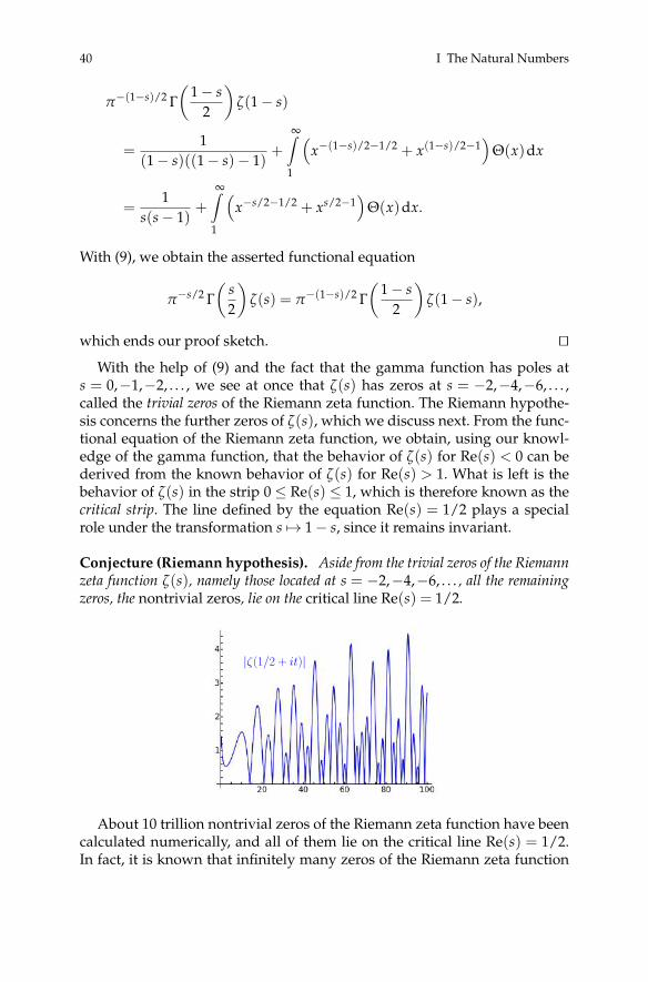
40 I The Natural Numbers
π−(1−s)/2 Γ(
1− s2
)ζ(1− s)
=1
(1− s)((1− s)− 1)+
∞∫1
(x−(1−s)/2−1/2 + x(1−s)/2−1
)Θ(x)dx
=1
s(s− 1)+
∞∫1
(x−s/2−1/2 + xs/2−1
)Θ(x)dx.
With (9), we obtain the asserted functional equation
π−s/2 Γ(
s2
)ζ(s) = π−(1−s)/2 Γ
(1− s
2
)ζ(1− s),
which ends our proof sketch. utWith the help of (9) and the fact that the gamma function has poles at
s = 0,−1,−2, . . . , we see at once that ζ(s) has zeros at s = −2,−4,−6, . . . ,called the trivial zeros of the Riemann zeta function. The Riemann hypothe-sis concerns the further zeros of ζ(s), which we discuss next. From the func-tional equation of the Riemann zeta function, we obtain, using our knowl-edge of the gamma function, that the behavior of ζ(s) for Re(s) < 0 can bederived from the known behavior of ζ(s) for Re(s) > 1. What is left is thebehavior of ζ(s) in the strip 0 ≤ Re(s) ≤ 1, which is therefore known as thecritical strip. The line defined by the equation Re(s) = 1/2 plays a specialrole under the transformation s 7→ 1− s, since it remains invariant.
Conjecture (Riemann hypothesis). Aside from the trivial zeros of the Riemannzeta function ζ(s), namely those located at s = −2,−4,−6, . . . , all the remainingzeros, the nontrivial zeros, lie on the critical line Re(s) = 1/2.
|ζ(1/2 + it)|
About 10 trillion nontrivial zeros of the Riemann zeta function have beencalculated numerically, and all of them lie on the critical line Re(s) = 1/2.In fact, it is known that infinitely many zeros of the Riemann zeta function

A. Prime Numbers: Facts and Conjectures 41
lie on the critical line. For example, the locations of the zeros of the function|ζ(1/2 + it)| in the range 0≤ t ≤ 100 are shown in the preceding graph.
The Riemann hypothesis remains to this day an open problem, and it isone of the most important, if not the most important, conjectures in num-ber theory. It is one of the six remaining unsolved Millennium Problems.Its proof would have a host of implications. In particular, the vast numberof theorems that have been proved conditionally on the validity of the Rie-mann hypothesis would at once become unconditional proofs.
A weak form of the Riemann hypothesis is given by the Lindelöf hypoth-esis (after Ernst Leonard Lindelöf), which also has defied all attempts atproof.
Conjecture (Lindelöf hypothesis [5]). For every ε > 0, we have the followingestimate for t� 1:
ζ
(12+ it
)= o(tε).
Ralf Backlund a doctoral student of Ernst Lindelöf, showed that the Lin-delöf hypothesis is equivalent to the statment
#{
s ∈C | ζ(s) = 0, Re(s) ≥ 1/2 + ε, T ≤ Im(s) ≤ T + 1}= o(log(T)).
All that is known as of today is that the last quantity above is bounded byO(log(T)) for T� 1.
A.5 The Goldbach Conjecture
By the fundamental theorem of arithmetic, Theorem 3.1, the prime numbersare the multiplicative building blocks of the natural numbers. If we nowbring into play the other fundamental operation on the natural numbers,namely addition, there arise numerous questions that are not always easyto answer. One of the most famous problems of this sort goes back to a 1742exchange of letters between Christian Goldbach and Leonhard Euler, wherethe question was raised whether it is possible to express every natural num-ber greater than 5 as a sum of three primes. The following equivalent formis known as the Goldbach conjecture.
Conjecture (Goldbach conjecture). Every even number greater than 2 can bewritten as the sum of two primes.
This conjecture remains to this day only a conjecture, having withstoodnumerous attempts to prove it. Nonetheless, some progress has been madein the course of trying to prove the full conjecture. It is known, for example,

42 I The Natural Numbers
that every natural number greater than 6 can be written as the sum of dis-tinct primes. A breakthrough was obtained by the Peruvian mathematicianHarald Helfgott, who in 2013 announced a proof of the following weakerconjecture, known as the ternary Goldbach conjecture [3].
Conjecture (Ternary Goldbach conjecture). Every odd number greater than 5can be written as the sum of three primes.
For his proof, Helfgott used the fact that it was already known thatthe ternary Goldbach conjecture is true for all odd numbers greater than2 · 101346. Then, with the help of computers, he was able to verify the con-jecture for odd numbers less than 1027. The proof was then reduced to es-tablishing the conjecture for odd numbers in the interval between those twonumbers. Helfgott was able to do this using methods of analytic numbertheory, namely a refinement of the circle method, which goes back to God-frey Harold Hardy, John Littlewood, and Ivan Vinogradov.
With this, we complete our brief tour of questions surrounding the primenumbers. For more on primes, we refer the interested reader to the vast lit-erature on the subject. A good introduction can be found in the book [7], byPaulo Ribenboim, and the review article [11] by Don Zagier.
References
[1] H. M. Edwards: Riemann’s zeta function. Dover, New York, 2001.[2] J. Hadamard: Sur la distribution des zéros de la fonction ζ(s) et ses conséquences
arithmétiques. Bull. Soc. Math. de France 24 (1896), 199–220.[3] H. A. Helfgott: The ternary Goldbach conjecture is true. Preprint, December 30,
2013. Available online at arXiv:1312.7748.[4] J. Jones, D. Sato, H. Wada, D. Wiens: Diophantine representation of the set of prime
numbers. Amer. Math. Monthly 83 (1976), 449–464.[5] E. Lindelöf: Le calcul des résidus et ses applications dans la théorie des fonctions.
Gauthier-Villars, Paris, 1905.[6] Y. Matiyasevich: A Diophantine representation of the set of prime numbers. Dokl.
Akad. Nauk. SSSR 196 (1971), 770–773. English translation by R. N. Goss inSoviet Math. Dokl. 12 (1971), 249–254.
[7] P. Ribenboim: The little book of bigger primes. Springer, Berlin Heidelberg NewYork, 2004.
[8] B. Riemann: Ueber die Anzahl der Primzahlen unter einer gegebenen Grösse.Monatsberichte der Königlichen Preußischen Akademie der Wissenschaftenzu Berlin aus dem Jahre 1859 (1860), 671–680. In: Gesammelte Werke, Teub-ner, Leipzig, 1892. English translation by David R. Wilkins available online atwww.claymath.org/sites/default/files/ezeta.pdf.
[9] C.-J. de la Vallée Poussin: Recherches analytiques de la théorie des nombres premiers.Ann. Soc. Scient. Bruxelles 20 (1896), 183–256.
[10] I. M. Vinogradov: A new estimate of the function ζ(1+ it). Izv. Akad. Nauk. SSSRSer. Mat. 22 (1958), 161–164.

A. Prime Numbers: Facts and Conjectures 43
[11] D. Zagier: The first 50 million prime numbers. Math. Intel. 0 (1977), 221–224.[12] Y. Zhang: Bounded gaps between primes. Ann. of Math. (2) 179 (2014), 1121–1174.
II The Integers
1. Semigroups and Monoids
In Chapter I, we learned about the natural numbers with the operations ofaddition and multiplication. We may think about addition and multiplica-tion as processes whereby we take two natural numbers m1,m2 and formanother natural number, namely the sum m1 + m2 or the product m1 · m2.We may formalize this idea by saying that the set of natural numbers has de-fined on it the operations + and · that assign to two natural numbers m1,m2the respective natural numbers m1 + m2 and m1 · m2. If we let N ×N de-note the set of all ordered pairs of natural numbers, called the Cartesianproduct of N with itself, we may consider the operations of addition andmultiplication to be mappings from N×N to N given by the assignments(m1,m2) 7→ m1 + m2 and (m1, m2) 7→ m1 ·m2.
In what follows, we shall investigate the idea of a nonempty set M onwhich an operation ◦M is defined. In this case, we have a mapping fromM×M to M given by the assignment (m1,m2) 7→ m1 ◦M m2.
Generalizing the associativity of addition and multiplication of naturalnumbers, we call an operation ◦M on a set M associative if for all elementsm1,m2,m3 of M, we have
(m1 ◦M m2) ◦M m3 = m1 ◦M (m2 ◦M m3).
If we are given an associative operation ◦M on M, we can perform the op-eration on three elements m1,m2,m3 either by operating on the first two andthen operating on that result with the third, or by operating on the last twoand then operating on the first with that result. We may therefore write sim-ply m1 ◦M m2 ◦M m3.
Definition 1.1. A nonempty set H with an associative operation ◦H is calleda semigroup.
For such a semigroup, we write (H,◦H). If the context makes clear theconnection with H, we may write simply (H,◦). If it is clear that we aredealing with a semigroup, we may suppress reference to the operation andwrite simply H.
Example 1.2. (i) The natural numbers N with addition and with multi-plication forms the semigroups (N,+) and (N, ·).
(ii) Let A be an arbitrary nonempty set. On the set
© Springer International Publishing AG 2017
Springer Undergraduate Mathematics Series, https://doi.org/10.1007/978-3-319-69429-0_2J. Kramer and A.-M. von Pippich, From Natural Numbers to Quaternions,

46 II The Integers
map(A) := { f | f : A −→ A}
of all mappings of A to itself, we define the operation ◦ of compositionof mappings, which is well known to be associative. With this operation,(
map(A),◦)
is a semigroup.(iii) Let n be a nonzero natural number. Consider the subset
Rn := {0, . . . ,n− 1}
of the natural numbers comprising the first n natural numbers. On the setRn, we can define two operations. Let us denote by Rn(c) the remainderresulting from the division of a natural number c by n; that this number isuniquely determined is guaranteed by Theorem 5.1 of Chapter I. We observethat we have Rn(c) ∈ Rn. For two numbers a,b ∈ Rn, we now define themappings
⊕ :Rn ×Rn −→Rn, defined by a⊕ b := Rn(a + b), (1)� :Rn ×Rn −→Rn, defined by a� b := Rn(a · b). (2)
We leave it as an exercise for the reader to verify that the operations⊕ and�are associative (the associativity is derived from the associativity of additionand multiplication on the set of natural numbers). We thereby obtain twosemigroups, (Rn,⊕) and (Rn,�).
Exercise 1.3. Verify that the operations ⊕ and � from Example 1.2 (iii) areassociative.
Exercise 1.4.(a) Prove that the natural numbers with addition and with multiplication
form semigroups, while for the odd natural numbers, a semigroup arisesonly under multiplication.
(b) Find other proper subsets of the natural numbers N that form semi-groups under addition or multiplication.
Exercise 1.5. Does the set N of natural numbers under the operation of ex-ponentiation,
n ◦m := nm (m, n ∈N),
form a semigroup?
Definition 1.6. A semigroup (H,◦) is said to be commutative, or abelian, iffor all elements h1, h2 ∈ H, we have
h1 ◦ h2 = h2 ◦ h1.
The term abelian is in honor of the Norwegian mathematician Niels HenrikAbel.
1. Semigroups and Monoids 47
Example 1.7. The examples of semigroups (i) and (iii) above are both abelian.Example (ii) exhibits a semigroup that is in general nonabelian.
Exercise 1.8. Find two sets A1 and A2 such that (map(A1),◦) is an abeliansemigroup but (map(A2), ◦) is a nonabelian semigroup.
A modest generalization of the notion of semigroup leads to the conceptof a monoid.
Definition 1.9. A monoid is a semigroup (H,◦) that contains an identity ele-ment e with respect to the operation ◦, that is, an element such that
e ◦ h = h = h ◦ e
for every h ∈ H.
Lemma 1.10. The identity element e of a monoid (H,◦) is uniquely determined.
Proof. Let e, e′ be identity elements of the monoid (H,◦). By applying theidentity element e, we obtain the equality
e ◦ e′ = e′ = e′ ◦ e. (3)
If we now bring the identity element e′ into play, we obtain
e′ ◦ e = e = e ◦ e′. (4)
From equalities (3) and (4), we obtain at once the equality
e′ = e′ ◦ e = e.
This proves the uniqueness of the identity element. ut
Remark 1.11. We can refine Definition 1.9 of a monoid by requiring only theexistence of a left identity element e` (or right identity element er), which wouldsatisfy the respective conditions
e` ◦ h = h and h ◦ er = h
for all h ∈ H. However, it is easily shown that the left identity element isequal to the right identity element. We call such an element simply the iden-tity element. With the preceding lemma, we can see that H has exactly oneleft identity element and one right identity element and that those two ele-ments coincide.
Exercise 1.12. Let (H,◦) be a semigroup and e` a left identity element and era right identity element in H. Show that then e` = er.

48 II The Integers
Example 1.13. The examples of semigroups from Example 1.2 are all exam-ples of monoids:
(i) The identity element of N with respect to addition is 0; the identityelement ofNwith respect to multiplication is 1.
(ii) The identity element of(
map(A), ◦)
is the identity mapping idA :A −→ A, which maps every element a ∈ A to itself.
(iii) The identity element of Rn with respect to ⊕ is 0; the identity ele-ment ofRn with respect to � is 1.
Exercise 1.14.(a) Show that the even natural numbers form a monoid under addition, but
only a semigroup under multiplication.(b) Find other examples of semigroups that are not monoids.
2. Groups and Subgroups
We begin with the important definition of a group.
Definition 2.1. A monoid (G,◦) with identity element e is called a group iffor every g ∈ G, there exists an element g′ ∈ G such that
g′ ◦ g = e = g ◦ g′.
Such an element g′ is called an inverse element to g or simply an inverse of g.
Remark 2.2. In analogy to the uniqueness of the identity element of a monoid,one can show that the inverse g′ of an element g of a group G is uniquelydetermined. We may therefore speak of the inverse g′ of g ∈ G. The usualnotation for the inverse g′ of g ∈ G is g−1.
One can also refine Definition 2.1 of a group by requiring only the exis-tence of a left inverse g′` (or a right inverse g′r) for every g ∈ G, satisfying therespective conditions
g′` ◦ g = e (or g ◦ g′r = e).
But as before, it can be shown that if there is a left inverse, then there is also aright inverse, and they are equal. Such an element is called simply an inverseelement. We can then state that for every g ∈ G, there exists precisely one leftinverse and one right inverse in G and that those two elements coincide.
Exercise 2.3.(a) Prove that the inverse g−1 of an element g of a group (G,◦) is uniquely
determined.(b) Let (G,◦) be a group, g ∈ G, g′` a left inverse, and g′r a right inverse of g.
Show that g′` = g′r.
2. Groups and Subgroups 49
With the knowledge of the uniqueness of the identity element and in-verses, we may state the definition of a group as follows.
Definition 2.4. A group (G,◦) consists of a nonempty set G together withan associative operation ◦ such that the following two properties are satis-fied:(i) There exists a unique element e ∈ G such that
e ◦ g = g = g ◦ e
for all g ∈ G. The element e is the identity element of G.(ii) For each g ∈ G, there exists a uniquely determined element g−1 ∈ G
such thatg−1 ◦ g = e = g ◦ g−1.
The element g−1 is the inverse element to g.
Remark 2.5. For a group (G,◦) with identity element e and n ∈N, we intro-duce the following useful exponential notation for the n-fold operation ofan element g ∈ G on itself:
gn := g ◦ · · · ◦ g︸ ︷︷ ︸n times
and g0 := e. (5)
Exercise 2.6. Show that in the terminology of Remark 2.5, we have the fol-lowing rules of calculation:(a) (g−1)−1 = g for all g ∈ G.(b) (g ◦ h)−1 = h−1 ◦ g−1 for all g, h ∈ G.(c) gn ◦ gm = gn+m for all g ∈ G and n,m ∈N.(d) (gn)m = gn·m for all g ∈ G and n,m ∈N.
Definition 2.7. A group (G,◦) is called commutative or abelian if for all ele-ments g1, g2 ∈ G, we have
g1 ◦ g2 = g2 ◦ g1.
Example 2.8. (i) (G,◦) = (N,+) is not a group, since for no nonzero ele-ment n ∈ N does there exist a natural number n′ that satisfies the equationn′ + n = 0 = n + n′. That is, the nonzero natural numbers do not have (ad-ditive) inverses.
(ii) (G,◦) = (Rn,⊕) is a commutative group. If a ∈ Rn, a 6= 0, then theinverse to a is given by the difference n − a, where we note that indeed,n− a ∈ Rn.The semigroup (G,◦) = (Rn,�), on the other hand, is never a group, sincethe element 0 has no inverse. But even if we remove the zero element andconsider the semigroup (Rn \ {0},�), it is still not, in general, a group. If,
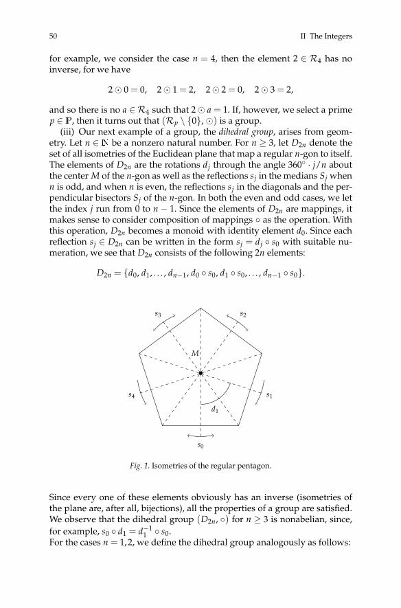
50 II The Integers
for example, we consider the case n = 4, then the element 2 ∈ R4 has noinverse, for we have
2� 0 = 0, 2� 1 = 2, 2� 2 = 0, 2� 3 = 2,
and so there is no a ∈ R4 such that 2� a = 1. If, however, we select a primep ∈ P, then it turns out that (Rp \ {0},�) is a group.
(iii) Our next example of a group, the dihedral group, arises from geom-etry. Let n ∈ N be a nonzero natural number. For n ≥ 3, let D2n denote theset of all isometries of the Euclidean plane that map a regular n-gon to itself.The elements of D2n are the rotations dj through the angle 360◦ · j/n aboutthe center M of the n-gon as well as the reflections sj in the medians Sj whenn is odd, and when n is even, the reflections sj in the diagonals and the per-pendicular bisectors Sj of the n-gon. In both the even and odd cases, we letthe index j run from 0 to n− 1. Since the elements of D2n are mappings, itmakes sense to consider composition of mappings ◦ as the operation. Withthis operation, D2n becomes a monoid with identity element d0. Since eachreflection sj ∈ D2n can be written in the form sj = dj ◦ s0 with suitable nu-meration, we see that D2n consists of the following 2n elements:
D2n = {d0, d1, . . . , dn−1, d0 ◦ s0, d1 ◦ s0, . . . , dn−1 ◦ s0}.
M
d1
s4
s3 s2
s1
s0
Fig. 1. Isometries of the regular pentagon.
Since every one of these elements obviously has an inverse (isometries ofthe plane are, after all, bijections), all the properties of a group are satisfied.We observe that the dihedral group (D2n, ◦) for n ≥ 3 is nonabelian, since,for example, s0 ◦ d1 = d−1
1 ◦ s0.For the cases n = 1,2, we define the dihedral group analogously as follows:

2. Groups and Subgroups 51
D2 := {d0, s0} and D4 := {d0,d1, s0,d1 ◦ s0}. We may interpret D2 and D4 assymmetry groups of the following 1-gon and 2-gon respectively:
Fig. 2. The 1-gon and 2-gon.
For n = 1,2, the dihedral group (D2n,◦) is abelian.(iv) As our last example, we consider a combinatorially based example
of a group, the nth symmetric group:
Sn ={
π∣∣π : {1, . . . , n} −→ {1, . . . ,n} and π is bijective
}.
The elements of Sn can be written in the convenient form
π =
(1 2 · · · n
π1 π2 · · · πn
),
where πj := π(j) for 1≤ j≤ n. For the associative operation on Sn, we againchoose composition of mappings; that is, for π,σ ∈ Sn, we have
π ◦ σ :=(
1 2 · · · nτ1 τ2 · · · τn
),
with τj := π(σ(j)
)for 1 ≤ j ≤ n. The identity element is the identity per-
mutation, given by the identity mapping on the set {1, . . . ,n}. Furthermore,the existence of the inverse of a permutation is guaranteed by the fact thatevery bijective mapping π : {1, . . . , n} −→ {1, . . . , n} has an inverse mappingπ−1. Under this operation, the set (Sn, ◦) forms a group, which for n ≥ 3 isnonabelian.
Exercise 2.9. (Cayley tables). For a finite group, the result of the group oper-ation on pairs of elements can be displayed in a Cayley table, named for theBritish mathematician Arthur Cayley, in which the elements of the group arelisted in the first row and first column of a table, and the remaining fieldsare filled in with the result of the group operation. For example, the Cayleytable for (R2,⊕) is as follows:
⊕ 0 10 0 11 1 0
Fig. 3. Cayley table for the group (R2,⊕)

52 II The Integers
Draw the Cayley tables for (R4,⊕), (R5 \ {0},�), (R6,⊕), (D4, ◦), and(D6, ◦), as well as for (S2, ◦) and (S3, ◦). What similarities and differencesdo you notice?
Exercise 2.10.(a) For the prime numbers p = 3 and p = 5, verify the assertion of Exam-
ple 2.8 (ii) that (Rp \ {0},�) is a group.(b) Verify in detail the assertions of Example 2.8 (iii) regarding the dihedral
group (D2n, ◦).(c) Think about why the symmetric group (Sn, ◦) from Example 2.8 (iv) is
nonabelian for all natural numbers n ≥ 3.
Definition 2.11. Let (G,◦) be a group. The cardinality of the set G underly-ing the group is called the order of G and is denoted by |G|. If the order of Gis infinite, we write |G| := ∞.
Example 2.12. For the groups in Example 2.8 (ii) and (iii), we have
|Rn| = n and |D2n| = 2n.
Exercise 2.13. Show that for the symmetric group (Sn, ◦), we have
|Sn| = n! .
Here n! for n ∈ N is the factorial function, defined inductively as follows:0! := 1, (n∗)! := n∗ · n!.
Definition 2.14. A group (G,◦) is said to be cyclic if there exists an elementg ∈ G such that
G = {. . . , (g−1)2, g−1, g0 = e, g1 = g, g2, . . .}.
In such a case, we write G = 〈g〉 and say that g generates the group G.
Example 2.15. The group (Rn,⊕) is generated by the element 1, that is, wehave (Rn,⊕) = 〈1〉, since every a ∈ Rn can be represented in the form
a = 1⊕ · · · ⊕ 1︸ ︷︷ ︸a times
.
Remark 2.16. Let G = 〈g〉 be a cyclic group of order n < ∞. Then we have
G = 〈g〉 = {e, g, g2, . . . , gn−1}.
This shows in particular that gn = e, gn+1 = g, etc.

2. Groups and Subgroups 53
Definition 2.17. Let (G,◦) be a group with identity element e and let g bean arbitrary element of G. The smallest nonzero natural number n such thatgn = e is called the order of g and is denoted by ordG(g). If there is no suchn ∈N, then the order of g is said to be infinite, that is, ordG(g) := ∞.
If the group to which the order of g refers is clear from context, then wewrite simply ord(g).
Example 2.18. We present here as an example the orders of the elements ofthe four-element group (R4,⊕):
ord(0) = 1, ord(1) = 4, ord(2) = 2, ord(3) = 4.
Exercise 2.19. Determine the orders of all elements of the group S3.
Remark 2.20. Let G = 〈g〉 be a cyclic group of order n<∞. Then ordG(g) = n.
Definition 2.21. Let (G,◦) be a group. A subset U ⊆ G is called a subgroupof G if the restriction ◦|U of the operation ◦ to U defines a group structure onU, that is, if (U, ◦|U) is itself a group. We express this relationship by writingU ≤ G.
Example 2.22. Let m, n be natural numbers with m ≤ n. Then the mth sym-metric group Sm is a subgroup of the nth symmetric group Sn if we identifya permutation in Sm with the corresponding permutation of Sn that leavesm + 1, . . . ,n fixed. That is, Sm ≤ Sn.
Exercise 2.23. Show that the rotations {d0, . . . , dn−1} form a cyclic subgroupof the dihedral group D2n.
Remark 2.24. Let (G,◦) be a group, and U a subgroup of G. The identityelement e of G is also the identity element of U. If h is an element of U, thenits inverse in U is given by the inverse of h in G, that is, by h−1, since
h ◦ |Uh−1 = h ◦ h−1 = e.
Lemma 2.25 (Subgroup criterion). Let (G,◦) be a group and U⊆G a nonemptysubset. Then we have the equivalence
U ≤ G ⇐⇒ h1 ◦ h−12 ∈U ∀h1, h2 ∈U.
Proof. (i) Suppose first that U is a subgroup of G. We must then show thatfor all h1, h2 ∈ U, we have the inclusion h1 ◦ h−1
2 ∈ U. But that is easy, sinceif h2 ∈ U, then we also have h−1
2 ∈ U, and by applying the group operationto h1 ∈U, we at once obtain h1 ◦ h−1
2 ∈U.(ii) Now suppose that conversely, h1 ◦ h−1
2 ∈ U for all h1, h2 ∈ U. Since Uis nonempty, there is at least one element h ∈ U, for which we then have

54 II The Integers
e = h ◦ h−1 ∈U. That is, U contains the identity element. If h′ is an arbitraryelement of U, we see that
h′−1 = e ◦ h′−1 ∈U.
That is, h′ ∈ U implies that h′−1 ∈ U. Finally, let h1 and h2 be arbitrary ele-ments of U. We must convince ourselves that the element h1 ◦ h2 is also in U.We recall that h2 ∈ U implies h−1
2 ∈ U. Using rule (a) from Exercise 2.6, weobtain
h1 ◦ h2 = h1 ◦(h−1
2)−1 ∈U.
We conclude that ◦ is an associative operation defined on U and that (U, ◦)satisfies all the group axioms. This completes the proof that U is a subgroupof G. ut
Exercise 2.26. Find all subgroups of the group S3. Which of these are cyclicgroups?
3. Group Homomorphisms
In this section, we are going to compare groups using mappings that respectthe group operation. The first thing, then, is to explain what is meant bypreserving the group operation, or group structure.
Definition 3.1. Let (G, ◦G) and (H, ◦H) be groups. A mapping
f : (G, ◦G) −→ (H, ◦H)
is called a group homomorphism if for all g1, g2 ∈ G, we have the equality
f (g1 ◦G g2) = f (g1) ◦H f (g2).
The significance of a homomorphism is, then, that the image under f of thecomposition of two elements g1 and g2 in G is equal to the composition ofthe images under f of g1 and g2 in H. We sometimes say that the mappingf preserves the group structure.
A bijective (that is, both injective and surjective) group homomorphism iscalled a group isomorphism. If f : (G, ◦G)−→ (H, ◦H) is a group isomorphism,we say that the groups G and H are isomorphic, and we write G ∼= H.
Example 3.2. Consider the dihedral group G = D6 and the symmetric groupH = S3. The dihedral group D6 consists of all symmetries of an equilateraltriangle4. Let us denote the vertices of4 in counterclockwise order by thenatural numbers 1, 2, 3. If we choose one of the symmetry mappings g ∈ D6and allow it to act on4, the result is a permutation π of the set {1, 2, 3}. Theassignment g 7→ π thereby induces a mapping

3. Group Homomorphisms 55
f : D6 −→ S3.
If we consider all possible compositions of symmetries and their images un-der f and compare them with the corresponding compositions of permuta-tions, we see that f is a group homomorphism.
Exercise 3.3. Is this mapping also a group isomorphism?
Definition 3.4. Let (G, ◦G) be a group with identity element eG, and let(H, ◦H) be a group with identity element eH . Furthermore, let f : (G, ◦G)−→(H, ◦H) be a group homomorphism. Then
ker( f ) := {g ∈ G | f (g) = eH}
is called the kernel of f , and
im( f ) := {h ∈ H | ∃g ∈ G : h = f (g)}
is called the image of f .
Exercise 3.5. Let D2n be the dihedral group from Example 2.8 (iii). In thatexample, we noted that every element can be expressed uniquely in theform dj ◦ sk
0 with j ∈ {0, . . . , n − 1} and k ∈ {0, 1}. Show that the mappingsgn : (D2n, ◦) −→ (R2,⊕), given by the assignment dj ◦ sk
0 7→ k, is a grouphomomorphism, and determine the kernel and image of sgn.
Lemma 3.6. Let f : (G, ◦G) −→ (H, ◦H) be a group homomorphism. Then wehave the following:(i) f is injective if and only if ker( f ) = {eG}.(ii) f is surjective if and only if im( f ) = H.
Proof. (i) By definition, the mapping f is injective if and only if for allg1, g2 ∈ G,
f (g1) = f (g2) (6)
implies that g1 and g2 are equal. We therefore take equality (6) and transformit by means of the group homomorphism property of f into the equivalentform
f (g1) ◦H(
f (g2))−1
= eH ⇐⇒ f (g1) ◦H f (g−12 ) = eH .
Applying again the group homomorphism property of f yields f (g1 ◦Gg−1
2 ) = eH , that is, g1 ◦G g−12 ∈ ker( f ). Finally, the equivalence
g1 ◦G g−12 = eG ⇐⇒ g1 = g2
shows that we have ker( f ) = {eG} if and only if g1 = g2, that is, if and onlyif f is injective.

56 II The Integers
(ii) The proof of this assertion is obvious, since the surjectivity of f meansprecisely that every element of H is the image of some element of G underthe mapping f . ut
Exercise 3.7. Let f : (G, ◦) −→ (G, ◦) be a group homomorphism and as-sume that |G| < ∞. Prove the equivalence
ker( f ) = {eG} ⇐⇒ f is a group isomorphism.
Exercise 3.8. Let f : (G, ◦G) −→ (H, ◦H) be a group homomorphism. Showthat for every element g ∈ G, we have ordG(g) ≥ ordH
(f (g)
).
Exercise 3.9. Does there exist a group isomorphism between D24 and S4?
Lemma 3.10. Let f : (G, ◦G) −→ (H, ◦H) be a group homomorphism. Thenker( f ) is a subgroup of G, and im( f ) is a subgroup of H.
Proof. We begin with the proof that ker( f ) is a subgroup of G. We first ob-serve that because we have f (eG) = eH , that is, eG ∈ ker( f ), the kernel of f isnonempty. We now apply the subgroup criterion (Lemma 2.25). To this end,we choose g1, g2 ∈ ker( f ) and must show that g1 ◦G g−1
2 ∈ ker( f ). But thisfollows easily from the homomorphism property of f :
f (g1 ◦G g−12 ) = f (g1) ◦H f (g−1
2 ) = eH ◦H(
f (g2))−1
= eH ◦H e−1H = eH .
To prove the subgroup property of im( f ), we proceed analogously. Again,since eH = f (eG), that is, eH ∈ im( f ), the image of f is nonempty. We againmake use of the subgroup criterion and must establish for h1, h2 ∈ im( f )the relationship h1 ◦H h−1
2 ∈ im( f ). Since h1, h2 ∈ im( f ), there exist g1, g2 ∈G such that h1 = f (g1) and h2 = f (g2). Again using the homomorphismproperty of f yields
h1 ◦H h−12 = f (g1) ◦H
(f (g2)
)−1= f (g1) ◦H f (g−1
2 ) = f (g1 ◦G g−12 );
that is, the element h1 ◦H h−12 is the image of the element g1 ◦G g−1
2 . Thiscompletes the proof of the lemma. ut
Exercise 3.11.(a) Find all group homomorphisms f : (R4,⊕) −→ (R4,⊕).(b) Let p be a prime number and n∈N a natural number that is not divisible
by p. Find all group homomorphisms g : (Rp,⊕) −→ (Rn,⊕).Determine the image and kernel of each homomorphism.

4. Cosets and Normal Subgroups 57
4. Cosets and Normal Subgroups
Before we introduce the notion of a coset (with respect to a subgroup), werecall the definition of an equivalence relation.
Definition 4.1. Let M be a set. A (binary) relation∼ on M is called an equiv-alence relation if the following three conditions are satisfied:(i) The relation ∼ is reflexive, that is, for all m ∈ M, we have m ∼ m.(ii) The relation ∼ is symmetric, that is, for all m1, m2 ∈ M such that m1 ∼
m2, we have also m2 ∼ m1.(iii) The relation ∼ is transitive, that is, for all m1, m2, m3 ∈ M such that
m1 ∼ m2 and m2 ∼ m3, we have also m1 ∼ m3.
Example 4.2. The equality “=” of elements of a set defines an equivalencerelation.
Exercise 4.3.(a) Verify the assertion of Example 4.2.(b) Is the order relation ≤ onN an equivalence relation?(c) Consider a relation ∼ on the set of natural numbers N whereby m ∼ n
if m is a power of n or n is a power of m. Determine whether ∼ is anequivalence relation.
Remark 4.4. Let M be a set equipped with an equivalence relation ∼. Foreach m ∈ M, we can construct the set
Mm := {m′ ∈ M | m′ ∼ m}.
The set Mm is called the equivalence class of m.
Lemma 4.5. Let M be a set equipped with an equivalence relation ∼. Then wehave the following:(i) Two equivalence classes in M are either disjoint or identical.(ii) The set M is the disjoint union of its equivalence classes. We indicate this by
writingM =
⋃m∈I
Mm,
where I ⊆ M is a subset containing exactly one representative from eachequivalence class.
Proof. (i) Let m1, m2 ∈ M be such that Mm1 ∩Mm2 6= ∅, where ∅ is the stan-dard notation for the empty set. We must show that Mm1 = Mm2 . SinceMm1 ∩ Mm2 6= ∅, there exists m ∈ Mm1 ∩ Mm2 ; that is, we have m ∼ m1and m ∼ m2, and therefore, by the symmetry and transitivity of the equiv-alence relation ∼, we have m1 ∼ m2, whence we have m1 ∈ Mm2 . It fol-lows by another application of transitivity that we likewise have m′ ∈ Mm2

58 II The Integers
for all m′ ∈ Mm1 . We see, then, that Mm1 ⊆ Mm2 . Interchanging the rolesof the equivalence classes Mm1 and Mm2 , we obtain the reverse inclusionMm2 ⊆ Mm1 , from which follows the equality Mm1 = Mm2 .
(ii) To prove the second part of the assertion, we begin with the case thatM is a finite set. In this case, we can proceed constructively. If M is empty,then there is nothing to prove. Otherwise, there exists m1 ∈M with its equiv-alence class Mm1 . The set-theoretic difference M \Mm1 is now either empty,that is, M = Mm1 , or there exists m2 ∈ M \Mm1 with equivalence class Mm2 .We have now the two alternatives
M = Mm1 ∪Mm2 and ∃ m3 ∈ M \ (Mm1 ∪Mm2).
Since the set M is finite, this process must end after finitely many steps, sayk steps, and we obtain M as the disjoint union
M =k⋃
j=1
Mmj .
Now that we have illustrated the proof in the case of finite sets, let us turnour attention to the general situation. Since the equivalence class Mm asso-ciated with m ∈ M contains the element m, it is clear that M is the union ofall its equivalence classes. That is,
M =⋃
m∈MMm.
This union, however, is not in general disjoint. By selecting a unique rep-resentative of each equivalence class, we obtain a subset I ⊆ M such thatfor each m ∈ I, the associated equivalence class Mm in the above union ap-pears exactly once. The subset I is called a complete set of equivalence classrepresentatives. We thereby obtain the representation of M as the disjointunion
M =⋃
m∈IMm ,
as asserted. ut
Exercise 4.6. Describe the equivalence classes of the equality relation “=”from Example 4.2. Come up with other equivalence relations and determinethe associated equivalence classes.
We now introduce a particular equivalence relation on a group inducedby a subgroup.
Remark 4.7. Let (G,◦) be a group, and U ≤ G a subgroup. We define on Gthe relation

4. Cosets and Normal Subgroups 59
g1 ∼ g2 ⇐⇒ g−11 ◦ g2 ∈U (g1, g2 ∈ G).
We assert that this defines an equivalence relation on G. The reflexivity g∼ gis immediate from the fact that g−1 ◦ g = e ∈U. If g1 ∼ g2, whence g−1
1 ◦ g2 ∈U, it follows by taking inverses that
U 3 (g−11 ◦ g2)
−1 = g−12 ◦ g1.
That is, g2 ∼ g1, which proves symmetry. Finally, if we have g1 ∼ g2 andg2 ∼ g3, whence g−1
1 ◦ g2 ∈ U and g−12 ◦ g3 ∈ U, it follows by composition
thatU 3 (g−1
1 ◦ g2) ◦ (g−12 ◦ g3) = g−1
1 ◦ g3,
that is, g1 ∼ g3, which establishes transitivity.
Definition 4.8. Let (G,◦) be a group, U ≤ G a subgroup, and ∼ the equiv-alence relation from Remark 4.7. We call the equivalence class of g ∈ G, thatis, the set of group elements
{g′ ∈ G | g′ ∼ g},
the left coset of g with respect to the subgroup U. From the equivalence
g′ ∼ g ⇐⇒ g−1 ◦ g′ ∈U ⇐⇒ ∃h ∈U : g′ = g ◦ h,
we obtain{g′ ∈ G | g′ ∼ g} = {g ◦ h | h ∈U}.
We may therefore denote the left coset of g with respect to U simply by g ◦U.
Remark 4.9. Let (G,◦) be a group, U≤ G a subgroup, and∼ the equivalencerelation from Remark 4.7. Then using Lemma 4.5, we obtain a decomposi-tion of G into disjoint left cosets; that is,
G =⋃g∈I
g ◦U,
where I ⊆ G is a complete set of representatives of all left cosets with respectto U.
Definition 4.10. Let (G,◦) be a group and U ≤ G a subgroup. We denoteby G/U the set of all left cosets of elements of G with respect to U, that is,
G/U = {g ◦U | g ∈ I},
where I ⊆ G is a complete set of representatives of all left cosets with respectto U.
60 II The Integers
Exercise 4.11. Let m, n be natural numbers with 1≤ m ≤ n. Find a completeset of representatives of the set of left cosets Sn/Sm.
Exercise 4.12. From among the subgroups of S3 determined in Exercise 2.26,choose a subgroup of order two and determine all left cosets of S3 with re-spect to this subgroup.
Lemma 4.13. Let (G,◦) be a group, and U ≤ G a subgroup. All left cosets of Gwith respect to U have the same order as the subgroup U.
Proof. Let g ◦ U be the left coset of g with respect to U, and consider themapping
ϕ : g ◦U −→U,
given by g ◦ h 7→ h (h ∈ U). The assignment h 7→ g ◦ h clearly induces theinverse mapping to ϕ, namely ϕ−1. We see, then, that ϕ is bijective, fromwhich it follows that g ◦U and U have the same order. That is, we have theequality
|g ◦U| = |U|,as asserted. ut
Theorem 4.14 (Lagrange’s theorem). Let (G,◦) be a finite group (that is, |G|<∞), and let U ≤ G be a subgroup. Then the order of U divides the order of G, thatis, |U| | |G|.
Proof. Since the group G is finite, it can be decomposed into finitely manyleft cosets with respect to U. That is, we have a disjoint decomposition of theform
G = (g1 ◦U) ∪ · · · ∪ (gk ◦U).
Since the left cosets gj ◦U (j = 1, . . . ,k) are mutually disjoint and each of theirorders is equal to |U| by Lemma 4.13, we obtain
|G| =k
∑j=1|gj ◦U| = k · |U|.
This completes the proof of the theorem. ut
Exercise 4.15.(a) Derive from Lagrange’s theorem the fact that in a finite group, the order
of each element is a divisor of the order of the group.(b) Conclude from part (a) that a group whose order is a prime number
must be cyclic.(c) Determine all possible groups of orders 4 and 6 up to isomorphism.

4. Cosets and Normal Subgroups 61
Definition 4.16. Let (G,◦) be a group, and U ≤ G a subgroup. The order ofG/U is called the index of U in G and is denoted by [G : U].
Remark 4.17. If (G,◦) is a finite group and U≤G a subgroup, it follows fromthe proof of Lagrange’s theorem that the order of G is equal to the productof the order of U and the index of U in G. That is, we have
|G| = [G : U] · |U|.
In analogy to the left cosets, we can, of course, construct the set of rightcosets.
Remark 4.18. Let (G,◦) be a group, and U ≤ G a subgroup. We define on Gthe additional relation
g1 ∼r g2 ⇐⇒ g1 ◦ g−12 ∈U (g1, g2 ∈ G).
We leave it as an exercise to the reader to show that this defines an equiva-lence relation on G. The equivalence class of g ∈ G is called the right coset ofg with respect to U. This leads to the following:
{g′ ∈ G | g′ ∼r g} = {h ◦ g | h ∈U} =: U ◦ g.
We have thus obtained a decomposition of G into disjoint right cosets; thatis,
G =⋃
g∈Ir
U ◦ g,
where Ir ⊆ G is a complete system of right coset representatives with respectto U.
We denote the set of right cosets with respect to U by U\G. Just as in thecase of left cosets, all the right cosets of G with respect to U have the sameorder as the subgroup U.
Finally, it is easy to verify that by associating the left coset g ◦U with theright coset U ◦ g−1, we induce a bijection between the sets G/U and U\G.That is, we have
|G/U| = [G : U] = |U\G|.If the group G is abelian, then the left and right cosets coincide.
Exercise 4.19. Solve Exercises 4.11 and 4.12 for right cosets.
Definition 4.20. Let (G,◦) be a group. A subgroup N of G is said to be anormal subgroup if all left and right cosets with respect to N coincide, that is,if for all g ∈ G, we have g ◦ N = N ◦ g.
Since left and right cosets with respect to a normal subgroup N coincide,we speak in this case simply of cosets. If N ≤ G is a normal subgroup, thenwe indicate this fact by writing N E G.

62 II The Integers
Exercise 4.21. Is the subgroup chosen in Exercise 4.12 normal?
Remark 4.22. The following is equivalent to the definition above: A sub-group N of G is normal if and only if for every g ∈ G, we have
g ◦ N ◦ g−1 = N,
whereg ◦ N ◦ g−1 = {g′ ∈ G | g′ = g ◦ h ◦ g−1 with h ∈ N}.
We have yet another equivalent description of a normal subgroup: a sub-group N of G is normal if and only if for all g ∈ G and h ∈ N, we haveg ◦ h ◦ g−1 ∈ N. We can see that this definition is equivalent to the previ-ous one: We note first that we clearly have g ◦ N ◦ g−1 ⊆ N for all g ∈ G.To prove the reverse inclusion, we observe that from g ◦ h ◦ g−1 ∈ N for allg ∈ G, h ∈ N, we have in particular that g−1 ◦ h ◦ g ∈ N for all g ∈ G, h ∈ N.From this we conclude that g−1 ◦ N ◦ g ⊆ N for all g ∈ G. By operating onthis relation on the left by g and on the right by g−1, we obtain
N = g ◦ (g−1 ◦ N ◦ g) ◦ g−1 ⊆ g ◦ N ◦ g−1,
which is precisely the desired reverse inclusion. Therefore, we have indeedthe equality g ◦ N ◦ g−1 = N for all g ∈ G.
Example 4.23. We now consider the example of a normal subgroup of thesymmetric group S3. The reader will recall that S3 is given by the six permu-tations
S3 = {π1, π2, π3, π4, π5, π6},where
π1 =
(1 2 31 2 3
), π2 =
(1 2 32 3 1
), π3 =
(1 2 33 1 2
),
π4 =
(1 2 31 3 2
), π5 =
(1 2 33 2 1
), π6 =
(1 2 32 1 3
).
The three permutations π1, π2, π3 form a cyclic subgroup of order 3, de-noted by A3 = 〈π2〉 and called the alternating group of degree 3. We shall nowprove that A3 is a normal subgroup of S3. For j = 1, 2, 3, we have the obviousequality
πj ◦ A3 = A3 = A3 ◦ πj.
An explicit calculation with the element π4 shows that
π4 ◦ A3 = {π4 ◦ π1, π4 ◦ π2, π4 ◦ π3} = {π4, π5, π6},A3 ◦ π4 = {π1 ◦ π4, π2 ◦ π4, π3 ◦ π4} = {π4, π6, π5},

5. Quotient Groups and the Homomorphism Theorem 63
which establishes the equality π4 ◦ A3 = A3 ◦ π4. One can perform a similarcalculation for j = 5, 6:
πj ◦ A3 = A3 ◦ πj,
which proves the normality of A3. Our calculations have shown furthermorethat the set of (left) cosets with respect to A3 is given by
S3/A3 = {A3, π4 ◦ A3}.
In particular, we see that
[S3 : A3] = |S3|/|A3| =63= 2.
Exercise 4.24. Let G be a group and H ≤ G a subgroup of index 2.(a) Show that H is a normal subgroup of G.(b) Give a surjective group homomorphism from G to the group (R2,⊕).
Lemma 4.25. Let f : (G, ◦G) −→ (H, ◦H) be a group homomorphism. Then thekernel ker( f ) of f is a normal subgroup of G.
Proof. For simplicity of notation, we shall write simply ◦ in place of both ◦Gand ◦H .
By Lemma 3.10, ker( f ) is a subgroup of G. It remains to prove the nor-mality property for ker( f ), namely that
g ◦ h ◦ g−1 ∈ ker( f )
for all g∈G and h∈ ker( f ). So let g∈G and h∈ ker( f ) be arbitrary elements.We observe that f (h) = eH . Using the homomorphism property of f , weobtain
f (g ◦ h ◦ g−1) = f (g) ◦ f (h) ◦ f (g−1) = f (g) ◦ eH ◦(
f (g))−1
= f (g) ◦ f (g)−1 = eH .
We have therefore g ◦ h ◦ g−1 ∈ ker( f ), and the lemma is proved. ut
Exercise 4.26. Let f : (S3, ◦) −→ (R3,⊕) be a group homomorphism. Showthat we must have f (π) = 0 for all π ∈ S3.
5. Quotient Groups and the Homomorphism Theorem
We shall now show how we can provide, in a natural way, the set G/N of(left) cosets of a group G with respect to a normal subgroup N with a groupstructure. As a rule, the structure of the group G/N will be in some respect

64 II The Integers
simpler than the structure of the group G. Studying the group G/N providesinformation about the structure of the group G.
Definition 5.1. Let (G,◦) be a group, and N E G a normal subgroup. Wedefine an operation • on the set of (left) cosets with respect to N as follows:
(g1 ◦ N) • (g2 ◦ N) := (g1 ◦ g2) ◦ N (g1, g2 ∈ G). (7)
This definition appears to depend on the choice of representatives g1 and g2for the cosets g1 ◦ N and g2 ◦ N. We shall show, however, in the followinglemma that the operation • is in fact independent of the choice of represen-tatives.
Lemma 5.2. Let (G,◦) be a group, and N E G a normal subgroup. Then theoperation • defined on G/N in Definition 5.1 is well defined.
Proof. Let g1, g′1 and g2, g′2 be representatives of the respective cosets g1 ◦ Nand g2 ◦ N. To prove that the operation (7) is independent of the choice ofrepresentatives, we must prove the equality
(g1 ◦ g2) ◦ N = (g′1 ◦ g′2) ◦ N.
Since g′1 ∈ g1 ◦ N, there exists h1 ∈ N such that g′1 = g1 ◦ h1; analogously, weobtain g′2 = g2 ◦ h2 for some h2 ∈ N. We now calculate, taking into accountthe associativity of ◦,
(g′1 ◦ g′2) ◦ N =((g1 ◦ h1) ◦ (g2 ◦ h2)
)◦ N = (g1 ◦ h1 ◦ g2) ◦ (h2 ◦ N)
=(
g1 ◦ (h1 ◦ g2))◦ N,
where in the last step, we used the equality h2 ◦N = N, which holds becausewe have h2 ∈ N. Since N is normal in G, there exists h′1 ∈ N such that h1 ◦g2 = g2 ◦ h′1. Substituting this in the previous equation yields, as asserted,
(g′1 ◦ g′2) ◦ N =(
g1 ◦ (g2 ◦ h′1))◦ N = (g1 ◦ g2) ◦ N;
here we have again used the associativity of ◦ and the equality h′1 ◦ N = N.This completes the proof of the lemma. ut
With the help of Lemma 5.2, we now have a well-defined operation,namely •, on the set G/N. The following proposition asserts that (G/N, •)is in fact a group.
Proposition 5.3. Let (G,◦) be a group, and N E G a normal subgroup. The setG/N of (left) cosets of G with respect to N together with the operation • forms agroup.

5. Quotient Groups and the Homomorphism Theorem 65
Proof. We begin by establishing that the set G/N is nonempty, which can beseen from the fact that it contains the coset eG ◦N = N, that is, the element N.The associativity of the operation • follows at once from that of the operation◦ on the group G. Namely, using the definition of • and Lemma 5.2, weobtain (
(g1 ◦ N) • (g2 ◦ N))• (g3 ◦ N)
=((g1 ◦ g2) ◦ N
)• (g3 ◦ N) =
((g1 ◦ g2) ◦ g3
)◦ N
=(
g1 ◦ (g2 ◦ g3))◦ N = (g1 ◦ N) •
((g2 ◦ g3) ◦ N
)= (g1 ◦ N) •
((g2 ◦ N) • (g3 ◦ N)
)for all g1, g2, g3 ∈ G. The identity element of G/N is given by N. Indeed, forevery coset g ◦ N ∈ G/N, we have
N • (g ◦ N) = (eG ◦ N) • (g ◦ N) = (eG ◦ g) ◦ N = g ◦ N,(g ◦ N) • N = (g ◦ N) • (eG ◦ N) = (g ◦ eG) ◦ N = g ◦ N.
Finally, the inverse element to g ◦ N is given by the coset g−1 ◦ N, for wehave
(g−1 ◦ N) • (g ◦ N) = (g−1 ◦ g) ◦ N = eG ◦ N = N,
(g ◦ N) • (g−1 ◦ N) = (g ◦ g−1) ◦ N = eG ◦ N = N.
Thus (G/N, •) satisfies all the properties of a group, and the lemma isproved. ut
Definition 5.4. Let (G,◦) be a group, and N E G a normal subgroup. Thegroup (G/N, •) is called the quotient group of G by the normal subgroup N.
Example 5.5. (i) In an abelian group G, every subgroup H is normal.Therefore, we can form the quotient group (G/H, •) for every subgroupH of G. Each such quotient group is abelian.
(ii) In Example 4.23, we proved that the alternating group A3 is a normalsubgroup of the symmetric group S3. We may therefore form the quotientgroup S3/A3, which (in the notation of Example 4.23) consists of the twoelements e := A3 and g := π4 ◦ A3. The element e is the identity element inS3/A3, and the element g satisfies the relation g • g = e. We may thereforeidentify the quotient group S3/A3 with the familiar group (R2,⊕), whichconsists of the elements 0 and 1, by mapping the element e to 0 and theelement g to 1. It is easy to see that this identification is a bijective group ho-momorphism from S3/A3 toR2. We have therefore the group isomorphism
(S3/A3, •) ∼= (R2,⊕).
66 II The Integers
Remark 5.6. Let f : (G, ◦G)−→ (H, ◦H) be a group homomorphism. Lemma4.25 asserts that ker( f ) is a normal subgroup of G. We may therefore formthe quotient group (G/ker( f ), •). We now define the mapping
π : (G, ◦G) −→ (G/ker( f ), •)
via g 7→ g ◦G ker( f ). The definition of the operation • now shows that
π(g1 ◦G g2) = (g1 ◦G g2) ◦G ker( f ) =(
g1 ◦G ker( f ))•(
g2 ◦G ker( f ))
= π(g1) • π(g2);
that is, the mapping π is a group homomorphism, and it is surjective. Thehomomorphism π is called the canonical group homomorphism.
Theorem 5.7 (Homomorphism theorem for groups). Let f : (G, ◦G) −→(H, ◦H) be a group homomorphism. Then f induces a uniquely determined in-jective group homomorphism
f :(G/ker( f ), •
)−→ (H, ◦H)
such that f(
g ◦G ker( f ))= f (g) for all g ∈ G. The statement of the theorem can
be illustrated by saying that the diagram
(G, ◦G)
π
��
f
''(G/ker( f ), •) ∃! f // (H, ◦H)
is commutative, that is, that we obtain the same result by applying the mapping fdirectly or by first applying π and then the mapping f .
Proof. To simplify notation, we define N := ker( f ), and furthermore, weshall write simply ◦ in place of ◦G and ◦H . By Lemma 4.25, N is a normalsubgroup of G. We thereby obtain the quotient group (G/N, •). We nowdefine a mapping f from (G/N, •) to (H, ◦H) as follows:
f (g ◦ N) := f (g) (g ∈ G).
Since we defined f in terms of a particular representative g of the coset g ◦N,we must show that f is well defined. To this end, let g′ ∈ G be an arbitraryrepresentative of the coset g ◦ N; that is, there exists h ∈ N such that g′ =g ◦ h. We then obtain
f (g′) = f (g ◦ h) = f (g) ◦ f (h) = f (g) ◦ eH = f (g),

5. Quotient Groups and the Homomorphism Theorem 67
which shows that the definition of f is independent of the choice of repre-sentative of g ◦ N.
In a further step, we show that f is a group homomorphism. Choose twoarbitrary cosets g1 ◦ N and g2 ◦ N in G/N, and using the definition of f andthe homomorphism f , calculate
f((g1 ◦ N) • (g2 ◦ N)
)= f
((g1 ◦ g2) ◦ N
)= f (g1 ◦ g2) = f (g1) ◦ f (g2)
= f (g1 ◦ N) ◦ f (g2 ◦ N).
This shows that f is in fact a homomorphism.In a third step, we show the injectivity of f . Let g1 ◦ N, g2 ◦ N ∈ G/N be
such that f (g1 ◦ N) = f (g2 ◦ N). We have to show that g1 ◦ N = g2 ◦ N. Bydefinition, this proposed equality is equivalent to the equality f (g1) = f (g2).If we apply f (g1)
−1 to both sides of this equality from the left, we obtain
eH = f (g1)−1 ◦ f (g1) = f (g1)
−1 ◦ f (g2) = f (g−11 ◦ g2);
that is, we have g−11 ◦ g2 ∈ ker( f ) = N. This yields at once that g2 is an ele-
ment of the coset g1 ◦ N, that is, g2 ∼ g1. We have, therefore, the equality
g1 ◦ N = g2 ◦ N,
as asserted. Putting all of this together, we have shown that
f : (G/ker( f ), •) −→ (H, ◦H)
is a well-defined injective group homomorphism. It remains to prove theuniqueness of f such that f
(g ◦ ker( f )
)= f (g) (g ∈ G). Let
f : (G/ker( f ), •) −→ (H, ◦H)
be another injective group homomorphism such that f(
g ◦ ker( f ))= f (g)
(g ∈ G). Then we have
f(
g ◦ ker( f ))= f (g) = f
(g ◦ ker( f )
)(g ∈ G),
which means precisely that the action of f is identical to the action of f on(G/ker( f ), •). That is, we have f = f , which proves the uniqueness of f .This completes the proof of the homomorphism theorem for groups. ut
Corollary 5.8. Let f : (G, ◦G)−→ (H, ◦H) be a surjective group homomorphism.Then f induces a uniquely determined group isomorphism
f :(G/ker( f ), •
) ∼= (H, ◦H)
such that f(
g ◦G ker( f ))= f (g) for all g ∈ G. ut

68 II The Integers
Example 5.9. We consider the symmetric group Sn and recall from linearalgebra that every permutation π can be written as a composition of trans-positions (i.e., permutations that interchange two elements and leave theothers fixed) and that while such a representation is not unique, the numberof transpositions that occur in the representation of a given permutation isalways even or always odd, and depending on which it is, we speak of apermutation as itself being either even or odd. We may therefore define themapping
f : (Sn, ◦) −→ (R2,⊕)by sending π to 0 if the permutation is even, and to 1 if it is odd. It is easilyverified that f is a surjective group homomorphism. The kernel ker( f ) off consists of the even permutations, that is, those that can be representedby an even number of transpositions. We call this subgroup the alternatinggroup of degree n and denote it by An. By Corollary 5.8, we obtain the groupisomorphism
(Sn/An, •) ∼= (R2,⊕).
Exercise 5.10. Generalize the above discussion to the case of Exercise 4.24.That is, construct a group isomormphism
(G/H, •) ∼= (R2,⊕)
for a subgroup H ≤ G of index 2.
From the homomorphism theorem for groups, one can deduce a numberof additional isomorphisms between groups. Here is a typical example.
Exercise 5.11. Let G be a group, and H, K E G normal subgroups in G suchthat K ⊆ H. Show that K is normal in H, and we have the isomorphism
(G/K)/(H/K) ∼= G/H.
6. Construction of Groups from Regular Semigroups
In Remark 1.26 of Chapter I, we noted the bothersome fact that in the semi-group (N, +), the equation
n + x = m
is not solvable for arbitrary m, n ∈ N. If m ≥ n, then the unique solution isgiven by the difference x = m− n. If, on the other hand, we have m < n, thenthere is no solution in the set of natural numbers. This difficulty will now beovercome by extending the semigroup (N, +) to a group (G, ◦G), by whichwe mean that N ⊆ G, and the restriction of the operation ◦G to the subsetN coincides with the operation of addition +. Under these conditions, the

6. Construction of Groups from Regular Semigroups 69
equation n + x = m becomes transformed as an equation in G to n ◦G x = m,which has the unique solution
x = n−1 ◦G m.
Since the solution x in the case of m < n cannot be a natural number, it mustreside in G \N, the complement ofN in G.
We may thus inquire more generally into the circumstances under whichit is possible to extend a semigroup (H, ◦H) to a group (G, ◦G), namely agroup G containing H such that the restriction of ◦G to H coincides withthe operation ◦H . The following definition of regular semigroup is the keyconcept.
Definition 6.1. A semigroup (H, ◦H) is said to be regular if for all elementsh, x, y ∈ H, we have the cancellation laws
h ◦H x = h ◦H y =⇒ x = y,x ◦H h = y ◦H h =⇒ x = y.
Remark 6.2. (i) If the regular semigroup (H, ◦H) is abelian, then we requireonly a single cancellation law in Definition 6.1.
(ii) A group (G, ◦G) is itself a regular semigroup, since applying the in-verse h−1 to h ◦G x = h ◦G y (h, x, y ∈ G) from the left yields
h−1 ◦G h ◦G x = h−1 ◦G h ◦G y ⇐⇒ x = y.
The other implication follows from applying the group operation with h−1
from the right.
Example 6.3. It is easy to show by mathematical induction that the semi-group (N, +) is regular. Because (N, +) is abelian, it suffices to prove theimplication
h + x = h + y =⇒ x = y (h, x, y ∈N). (8)
To this end, fix x, y ∈N and apply induction on h. For h = 0, the assertion isobviously correct, which establishes the basis of the induction. As inductionhypothesis, we assume that the implication (8) is true for some h ∈ N. Wemust then prove the implication
h∗ + x = h∗ + y =⇒ x = y
for the successor h∗ of h. From the equation
(h + x)∗ = h∗ + x = h∗ + y = (h + y)∗,

70 II The Integers
we obtain, on account of the injectivity of the successor mapping, that h +x = h + y, which yields x = y at once by the induction hypothesis. Sincex, y ∈ N were arbitrary, we have proved by induction the validity of thecancellation law in Definition 6.1 for all h, x, y ∈N.
Exercise 6.4.(a) Let A be a set with at least two elements. Show that neither of the two
cancellation laws holds in the semigroup (map(A), ◦).(b) Find other examples of semigroups that are not regular.
Theorem 6.5. For every regular abelian semigroup (H, ◦H) there exists a uniqueabelian group (G, ◦G) satisfying the following two conditions:(i) H is a subset of G, and the restriction of ◦G to H coincides with the opera-
tion ◦H .(ii) If (G′, ◦G′) is another group satisfying property (i), then G is a subgroup
of G′.
Proof. We must prove both existence and uniqueness. We begin with a proofof uniqueness.
Uniqueness: Let (G1, ◦G1) and (G2, ◦G2) be groups satisfying properties (i)and (ii). By property (ii), we have in particular that G1 ≤ G2, but converselyalso that G2 ≤ G1. That is, the two groups are identical. Therefore, the groupin question is determined uniquely (up to isomorphism).
Existence: We begin by defining a relation ∼ on the Cartesian product
H × H = {(a, b) | a, b ∈ H}
(for simplicity of notation, we shall write ◦ instead of ◦H):
(a, b) ∼ (c, d) ⇐⇒ a ◦ d = b ◦ c (a, b, c, d ∈ H).
We can easily show that this is an equivalence relation.(a) Reflexivity: Since the semigroup (H, ◦) is abelian, it follows that a ◦
b = b ◦ a for all a, b ∈ H. That is, (a, b) ∼ (a, b). Therefore, the relation ∼ isreflexive.
(b) Symmetry: Let (a, b), (c, d) ∈ H × H be such that (a, b) ∼ (c, d), thatis, a ◦ d = b ◦ c. Since (H, ◦) is abelian, we may conclude that c ◦ b = d ◦ a,which means precisely that (c, d) ∼ (a, b); that is, ∼ is symmetric.
(c) Transitivity: Let (a, b), (c, d), (e, f ) ∈ H× H be such that (a, b)∼ (c, d)and (c, d) ∼ (e, f ). We have, therefore, the equalities
a ◦ d = b ◦ c, c ◦ f = d ◦ e.
If we apply the group operation to the left-hand and right-hand sides ofthese two equations, we obtain, using the associativity and commutativityof the semigroup (H, ◦), the following equivalent equalities:

6. Construction of Groups from Regular Semigroups 71
(a ◦ d) ◦ (c ◦ f ) = (b ◦ c) ◦ (d ◦ e),a ◦ d ◦ c ◦ f = b ◦ c ◦ d ◦ e,
(a ◦ f ) ◦ (d ◦ c) = (b ◦ e) ◦ (d ◦ c).
Since the semigroup (H, ◦) is also regular, we can cancel (d ◦ c) in the lastequation (from the right), obtaining
a ◦ f = b ◦ e,
which implies (a, b) ∼ (e, f ). The relation ∼ is therefore also transitive.We denote by [a, b] ⊆ H × H the equivalence class of the pair (a, b) ∈
H × H, and by G the set of all such equivalence classes. For the sake ofbrevity, we write
G := (H × H)/ ∼ .
Since the semigroup (H, ◦) is nonempty, so that it contains at least one ele-ment h, it follows that the set G is also nonempty, since it contains at least theequivalence class [h, h]. We now define an operation on the set G of equiv-alence classes, which for simplicity we shall denote by • instead of ◦G. If[a, b], [a′, b′] ∈ G, then we define
[a, b] • [a′, b′] := [a ◦ a′, b ◦ b′].
Since this definition apparently depends on the choice of representatives a, band a′, b′ of the equivalence classes [a, b] and [a′, b′], we must prove that theoperation • is well defined by showing that it is, in fact, independent of thischoice. To this end, let (c, d) and (c′, d′) be arbitrary representatives of [a, b]and [a′, b′]. We must show that
[a ◦ a′, b ◦ b′] = [c ◦ c′, d ◦ d′] ⇐⇒ (a ◦ a′, b ◦ b′) ∼ (c ◦ c′, d ◦ d′).
Since we have (c, d) ∈ [a, b] and (c′, d′) ∈ [a′, b′], we must have
a ◦ d = b ◦ c and a′ ◦ d′ = b′ ◦ c′.
By composing the left- and right-hand sides, we obtain, on the assumptionof the commutativity of H,
(a ◦ d) ◦ (a′ ◦ d′) = (b ◦ c) ◦ (b′ ◦ c′)⇐⇒ (a ◦ a′) ◦ (d ◦ d′) = (b ◦ b′) ◦ (c ◦ c′),
and we have, therefore, as asserted,
(a ◦ a′, b ◦ b′) ∼ (c ◦ c′, d ◦ d′).
In sum, we now have in (G, •) a nonempty set with a well-defined op-eration. In the following four steps, we shall show that (G, •) is an abeliangroup.
72 II The Integers
(1) We first show that • is associative. But this can be shown easily fromthe definition of • and the associativity of ◦ with [a, b], [a′, b′], [a′′, b′′] ∈ G:
([a, b] • [a′, b′]) • [a′′, b′′] = [a ◦ a′, b ◦ b′] • [a′′, b′′]
= [(a ◦ a′) ◦ a′′, (b ◦ b′) ◦ b′′] = [a ◦ (a′ ◦ a′′), b ◦ (b′ ◦ b′′)]
= [a, b] • [a′ ◦ a′′, b′ ◦ b′′] = [a, b] • ([a′, b′] • [a′′, b′′]).
(2) The commutativity of • follows equally easily from the commutativ-ity of the operation ◦ with [a, b], [a′, b′] ∈ G:
[a, b] • [a′, b′] = [a ◦ a′, b ◦ b′] = [a′ ◦ a, b′ ◦ b] = [a′, b′] • [a, b].
(3) We now show that G possesses an identity element. To this end, wechoose an arbitrary element h ∈ H; we know that such an element exists,since H is nonempty. Then the equivalence class [h, h] is our candidate forthe identity element in G. Let [a, b] be an arbitrary element of G. By thecommutativity of ◦, we have
(h ◦ a) ◦ b = (h ◦ b) ◦ a ⇐⇒((h ◦ a), (h ◦ b)
)∼ (a, b).
Then from the commutativity of •, we obtain
[a, b] • [h, h] = [h, h] • [a, b] = [h ◦ a, h ◦ b] = [a, b].
That is, [h, h] is indeed the identity element in G.(4) Finally, we must show that every element [a, b] ∈ G has an inverse
[a, b]−1 in G. We assert that the desired inverse is given by [b, a] ∈ G. By thecommutativity of ◦ and •, we see that
[a, b] • [b, a] = [b, a] • [a, b] = [b ◦ a, a ◦ b] = [a ◦ b, a ◦ b].
Now, since the equality (a ◦ b) ◦ h = (a ◦ b) ◦ h is equivalent to (a ◦ b, a ◦ b)∼(h, h), we obtain the desired relation
[a, b] • [b, a] = [b, a] • [a, b] = [a ◦ b, a ◦ b] = [h, h].
To complete the proof, we must show that (G, •) satisfies the two condi-tions (i), (ii) above, namely (i) that H is a subset of G and the restriction of• to H coincides with the operation ◦, and (ii) that (G, •) is minimal withrespect to property (i).
To verify property (i), it suffices to find an injective mapping f : H −→ Gsatisfying
f (a ◦ b) = f (a) • f (b) (a, b ∈ H). (9)
By then identifying H with its image f (H) ⊆ G, we shall obtain, taking intoaccount (9), the desired result. We define the mapping f : H −→ G by send-ing each element a ∈ H to the element [a ◦ h, h] ∈ G (the element h was cho-

7. The Integers 73
sen when we defined the identity element [h, h] of G). We now show that fis injective. Let a, b ∈ H be such that
f (a) = f (b) ⇐⇒ [a ◦ h, h] = [b ◦ h, h] ⇐⇒ (a ◦ h, h) ∼ (b ◦ h, h).
Given the commutativity and regularity of (H, ◦), we see that this is equiv-alent to
(a ◦ h) ◦ h = h ◦ (b ◦ h) ⇐⇒ a ◦ h2 = b ◦ h2 ⇐⇒ a = b,
from which the injectivity of f follows.To prove (9), we choose two arbitrary elements a, b ∈ H and calculate,
taking into account the associativity and commutativity of ◦,
f (a ◦ b) = [(a ◦ b) ◦ h, h] = [a ◦ b ◦ h, h] = [a ◦ b ◦ h ◦ h, h ◦ h]= [(a ◦ h) ◦ (b ◦ h), h ◦ h] = [a ◦ h, h] • [b ◦ h, h] = f (a) • f (b).
We have thereby demonstrated the structure-preserving property (9) of f ,showing that (G, •) is an abelian group satisfying property (i).
To complete the proof, we show that the group (G, •) that we have con-structed is minimal. To this end, we show that the group (G, •) cannot bemade any smaller. By identifying, as mentioned above, the semigroup (H, ◦)with its image in (G, •) under f , we see that by construction, G must con-tain all elements of the form [a ◦ h, h] for a ∈ H. Since (G, •) is a group, itmust contain for each such [a ◦ h, h] the inverse [h, a ◦ h] in G; that is, G alsocontains all elements of the form [h, b ◦ h] with b ∈ H. Because G is closedunder the operation •, it must also contain all elements of the form
[a ◦ h, h] • [h, b ◦ h] = [a, b] (a, b ∈ H).
But this shows that one cannot omit a single equivalence class from G, show-ing that (G, •) is minimal. ut
Exercise 6.6.(a) Show that the odd natural numbers under multiplication form a regular
abelian monoid.(b) Carry out the construction for this monoid described in Theorem 6.5.
7. The Integers
We would like to investigate more closely the abelian group (G, ◦G) con-structed in Theorem 6.5 using the example of the regular abelian semigroup(H, ◦H) = (N, +). In doing so, we shall introduce the set of integers.
We begin by noting that the equivalence relation ∼ defined on the Carte-sian productN×N now assumes the form

74 II The Integers
(a, b) ∼ (c, d) ⇐⇒ a + d = b + c (a, b, c, d ∈N).
The abelian group (G, ◦G) is given, according to the proof of Theorem 6.5,by the set of all equivalence classes [a, b] associated with pairs (a, b)∈N×Nand is equipped with the operation
[a, b] ◦G [a′, b′] = [a + a′, b + b′] ([a, b], [a′, b′] ∈ G);
the identity element in (G, ◦G) is given by the element [0, 0], where 0 de-notes the natural number zero. Since we are dealing here with an additivestructure, we shall write the inverse [a, b]−1 in the form −[a, b].
The definition of the equivalence relation∼ shows in this special case thatevery equivalence class can be expressed in the form
[a, b] =
{[a− b, 0], if a ≥ b,[0, b− a], if b > a.
We see, then, that the underlying set G of the group (G, ◦G) is given by theunion
G = {[n, 0] | n ∈N} ∪ {[0, n] | n ∈N},where the intersection {[n, 0] | n ∈N} ∩ {[0, n] | n ∈N} consists solely of theidentity element [0, 0]. We see from the proof of Theorem 6.5 that the set ofnatural numbersN is in bijection with the set {[n, 0] | n ∈N}. This bijectionis induced by the assignment n 7→ [n, 0]. By identifying the set of naturalnumbers N with the set {[n, 0] | n ∈ N}, that is, we set n = [n, 0], we mayhenceforth viewN as a subset of G.
Definition 7.1. For a nonzero natural number n, we now set
−n := [0, n].
Taking into account the identification ofNwith {[n, 0] | n ∈N} and usingthe previous definition, we can realize G in the form
G = {0, 1, 2, 3, . . .} ∪ {−1,−2,−3, . . .}.
Definition 7.2. We shall hereinafter denote the group (G, ◦G) by (Z, +) andcall it the (additive) group of integers. As a set, we may represent Z in the form
Z= {. . . ,−3,−2,−1, 0, 1, 2, 3, . . .}.
We call the numbers 1, 2, 3, . . . positive integers, the numbers −1,−2,−3, . . .negative integers. Finally, for the integer given by the equivalence class [a, b],we introduce the usual notation
a− b := [a, b]
7. The Integers 75
and call it the difference of the natural numbers a and b.
Remark 7.3. (i) Definition 7.2, which defines the difference of two naturalnumbers, is unrestricted and therefore generalizes the notion of differencegiven in Definition 1.24 of Chapter I. Moreover, the general notion of differ-ence in Definition 7.2 is compatible with the notion of difference in Defini-tion 1.24 of Chapter I: if a, b ∈N with a ≥ b, then by Definition 7.2, we havea− b = [a, b]. Using Definition 1.24 of Chapter I, this can be transformed intoa− b = [a− b, 0]; the identification ofNwith {[n, 0] | n ∈N} now shows theasserted compatibility.
(ii) Since we denote the inverse [a, b] = a− b by−[a, b] =−(a− b), whichis in turn given by [b, a] = b− a, we obtain
−(a− b) = b− a.
If we set a = 0, we obtain in particular the formula −(−b) = b (b ∈N).(iii) Using (ii), we now obtain in general the difference of two integers
a− b = [a, b] and a′ − b′ = [a′, b′] in the form
(a− b)− (a′ − b′) := (a− b) +(− (a′ − b′)
)= (a− b) + (b′ − a′).
(iv) One should keep in mind in considering the difference a− b that thereis always an equivalence class lurking in the background; for example,
−2 = 1− 3 = 2− 4 = 3− 5 = · · · ;
that is, the pairs of natural numbers (1, 3), (2, 4), (3, 5), . . . are all represen-tatives of the integer −2 and of the equivalence class [0, 2].
Definition 7.4. We extend the relation ≤ on the set N of natural numbersgiven in Definition 1.15 of Chapter I to the set Z of integers by declaring thatevery negative integer is strictly less than every natural number and that fortwo negative integers −m,−n (m, n ∈N; m, n 6= 0), we set
−m < −n if m > n,−m ≤ −n if m ≥ n.
We extend the relations > and ≥ to the set Z of integers analogously.
In analogy to Remark 1.16 of Chapter I, we have the following.
Remark 7.5. With the relation <, the set of integers Z is an ordered set; thatis, the following conditions are satisfied:(i) For every two elements m, n ∈ Z, we have m < n or n < m or m = n.(ii) The three relations m < n, n < m, m = n are mutually exclusive.(iii) If m < n and n < p, then m < p.
76 II The Integers
Analogous properties hold for >.
Exercise 7.6. Generalize the addition and multiplication rules for the naturalnumbers in Remark 1.19 of Chapter I to the set of integers.
Definition 7.7. Let n ∈ Z be an integer. We then set
|n| :={
n, if n ≥ 0,−n, if n < 0.
We call the natural number |n| the absolute value of the integer n.
Example 7.8. The set of integers (Z, +) with the operation of addition thatwe have constructed gives us an additional example of an abelian group. Ifn ∈N is a nonzero natural number, then the set
nZ= {. . . ,−3n,−2n,−n, 0, n, 2n, 3n, . . .}
of all integral multiples of n forms a subgroup (nZ, +) of (Z, +). Since(Z, +) is an abelian group, the subgroup (nZ, +) will automatically bea normal subgroup of (Z, +), and we can consider the quotient group(Z/nZ, •).
Furthermore, we may easily verify that the assignment a 7→ Rn(a) (a ∈ Z)induces a group homomorphism
f : (Z, +) −→ (Rn,⊕).
This group homomorphism f is obviously surjective, and its kernel is
ker( f ) = nZ.
The corollary to the homomorphism theorem for groups yields for us thegroup isomorphism
(Z/nZ, •) ∼= (Rn,⊕);here the coset a + nZ ∈ Z/nZ is mapped to the element Rn(a) ∈ Rn. Thisexample demonstrates nicely how the complicated structure of the quotientgroup (Z/nZ, •) that we have been gradually developing can be identifiedwith the simple n-element setRn, on which we may perform “addition” bytaking remainders.
Exercise 7.9. Verify the assertions of this example in detail.
Remark 7.10. Theorem 6.5 applied to the regular abelian monoid (N \ {0}, ·)yields the multiplicative group of fractions (B, ·). We shall not discuss thegroup (B, ·) further, since in Section 6 of Chapter III, we shall rediscoverthis group as the multiplicative group of positive rational numbers.

B. RSA Encryption: An Application of Number Theory 77
B. RSA Encryption: An Application of Number Theory
In this final section, we shall discuss the ideas behind RSA encryption as aninteresting and current application of the properties of the integers.
B.1 Cryptography
The purpose of cryptography (from the Greek kryptos, hidden, and graphos,writing) is to maintain secrecy in communication so that unauthorized a-gents are unable to read or alter a message while it is being transmitted fromsender to receiver. The basic principle is simple. The unencrypted message,or plaintext, is transformed with the help of a key into a ciphertext that is nolonger comprehensible. Only someone in possession of the key can decryptthe ciphertext back into the original plaintext, thereby making the messageunderstandable.
The history of cryptography goes back at least to the second century B.C.,encrypted texts having been found as inscriptions on tombstones from thatperiod. We are not, however, going to delve into the history of the subject,for which we refer the reader to the relevant literature, some of which is of apopular nature (see, for example, [2, 7]). We shall instead touch on some ofthe basic ideas behind encryption algorithms.
In symmetric encryption algorithms, the keys for encryption and decryp-tion are essentially the same. For example, the key to such an algorithmmight consist in replacing each plaintext letter by a uniquely determinedciphertext letter.
A well-known example is the Caesar cipher, whereby the letters of the al-phabet in the top row are displaced cyclically by a certain number of places:
A B C D E F G H I J K L M N O P Q R S T U V W X Y Z
l l l l l l l l l l l l l l l l l l l l l l l l l lE F G H I J K L M N O P Q R S T U V W X Y Z A B C D
If, for example, that number of places is four, then the plaintext “HAIL CAE-SAR” would be encrypted as “LEMP GEIWEV,” as can be seen in the fol-lowing graphic, in which the plaintext letters appear in the outside ring,and their corresponding ciphertext letters can then be read off on the in-side ring. This variant of the Caesar cipher is quite simple, but the price ofthat simplicity is that it is a very insecure encryption technique, since for analphabet of twenty-six letters, there are only twenty-five different possiblekeys, so that without even the use of frequency analysis of the letters, theciphertext could be decrypted after at most the twenty-fifth attempt.

78 II The Integers
ZV
Y
U X
T WS
V
R
U
Q
T
P
S
O
R
N
QM
P
LO
K
N J
M I
L
HK
GJ
FI
EH
D
G
C
F
B
E
A
D
Z
C
YB
X
AWThe security of this method rested primarily, in the period when it was used,on the fact that the method of encryption was kept secret.
In modern cryptography, in contrast, a fundamental principle, calledKerckhoffs’s principle, after the Dutch linguist and cryptographer AugusteKerckhoffs, states that the security of an encryption algorithm should de-pend only on the security of the key and not on the secrecy of the algorithm.
A polyalphabetic modification of the Caesar cipher is the Vigenère cipher,named for Blaise de Vigenère, which uses an additional keyword to deter-mine the number of offset letters in the Caesar cipher. A popular conventionfor this method is that the letter A in the keyword represents no offset; theletter B, an offset of 1; the letter C, an offset of 2, and so on. If, for example,the supplementary keyword is “FANATIC,” then the alphabet for the firstletter to be encrypted is offset by 5; for the second letter, by 0; for the third, by13, and so on, 0, 19, 8, and 2. If the plaintext message is again “HAIL CAE-SAR,” then the ciphertext will read “MAVL VIGXAR.” While much moresecure than the Caesar cipher, this encryption method is truly secure onlyif the supplementary keyword is the same length as the plaintext, which ingeneral makes for a great deal of overhead.
Another variety of a polyalphabetic encryption algorithm is the basis ofthe famous Enigma code, which used a sort of electromechanical typewriter,making rapid encryption and decryption possible. The plaintext would beinput by keyboard. Then the letters of the plaintext were passed to three ro-tors, a reflector, and again three rotors, with the encrypted ciphertext finallydisplayed on a lamp board. The Enigma code was used by the Germans inthe Second World War, and was considered, incorrectly, to be unbreakable.
With the critical assistance of the mathematician Alan Turing, the Britishwere able to crack encrypted German radio messages beginning in about1940. An extensive description of Enigma, including its weaknesses and pos-sible improvements, can be found, for example, in [2] and in [7]. There arealso several enjoyable films on this topic, including the 2014 biopic “TheImitation Game.”
The reason that mathematics plays such an important role in cryptogra-phy is that there are many ways of encoding the information to be encryptedin the form of a number or sequence of numbers. For example, one can en-code the alphabet using ASCII encoding as follows:

B. RSA Encryption: An Application of Number Theory 79
A B C D E F G H I J K L M N O P Q R S T U V W X Y Z
l l l l l l l l l l l l l l l l l l l l l l l l l l65 66 67 68 69 70 71 72 73 74 75 76 77 78 79 80 81 82 83 84 85 86 87 88 89 90
Thus the text “HAIL CAESAR” corresponds in ASCII to the sequence
72, 65, 73, 76, 67, 65, 69, 83, 65, 82,
or simply to the number 72657376676569836582. Once the plaintext has beenwritten in the form of a number, encryption becomes a mathematical func-tion whose uniquely defined inverse is the function for decryption.
If in the ASCII coding above, we replace each number by its remainderon division by 26, we obtain the following encoding substitutions:
A B C D E F G H I J K L M N O P Q R S T U V W X Y Z
l l l l l l l l l l l l l l l l l l l l l l l l l l13 14 15 16 17 18 19 20 21 22 23 24 25 0 1 2 3 4 5 6 7 8 9 10 11 12
and now “HAIL CAESAR” will be encoded as 20,13,21,24,15,13,17,5,13,4.If we now employ a Caesar cipher with offset 4, the encryption function de-scribed above amounts to adding 4 to the corresponding number and sub-tracting 26 if the resulting number is greater than 25.
The plaintext 20,13,21,24,15,13,17,5,13,4 will therefore be encoded as24,17,25,2,19,17,9,17,8. Decryption involves simply applying the inversefunction, that is, subtracting the number 4 and then adding 26 if the result-ing number is negative. It is mathematically more elegant to describe theencryption function and its inverse in terms of congruences (modulo 26),which we shall learn about in Section B.2.
In the case of symmetric encryption procedures, it is easy in general toobtain the decryption function from knowledge of the encryption function,whence the name “symmetric.” There is, however, a fundamental problemregarding the security of symmetric encryption algorithms, namely to sendthe decryption function to the recipient of the ciphertext over a secure chan-nel. If an enemy can tap into the transmission and obtain the decryptionfunction, then the security of the ciphertext will have been compromised.
In 1976, Whitfield Diffie und Martin Hellman proposed in the article [4]that the problem of security might be solved by using two different keys,a public key for encryption, which is available to everyone, and a private keyfor decryption, which must remain secret, known only by the recipient ofthe ciphertext. This idea proved decisive for the transition from classicalcryptography to the modern concept of public key cryptography.
To realize this idea mathematically, the encryption function must have theproperty that an adversary would find it impossible to compute the inverse
80 II The Integers
function from knowledge of the encryption function without additional in-formation; even if the attacker could theoretically compute the inverse func-tion, it would take so long that in practice, it could not be done. For therecipient, however, who is in possession of the private key, computing theinverse function is easy. Moreover, the encryption function should have theadditional property that it is easy to convert plaintext to ciphertext, say inpolynomial time. Such a function is called a one-way trapdoor function.
The question of the existence of such a one-way trapdoor function re-mained long unresolved until three computer scientists, Ronald Rivest, AdiShamir, and Leonard Adleman, attempted to show that no such functioncould exist. But instead of doing so, they in fact discovered such a func-tion. In 1977, they produced an encryption algorithm known today by theinitials of their three surnames, the RSA algorithm, the first published asym-metric encryption algorithm; see [6]. Independently, similar ideas were de-veloped four years earlier by mathematicians in the British secret service,among them Clifford Cocks and James Ellis. Their work, however, was notpublished.
Today, the RSA algorithm is a widely used asymmetric procedure, withapplications in telephony, electronic banking, credit-card transactions, andin the Internet, for example in email encryption and transmission protocolssuch as TLS and SSH.
In the following sections, we provide a glimpse into how the RSA algo-rithm works along with the necessary elementary number theory. In partic-ular, we discuss congruence arithmetic, for which we shall need the theoryof divisibility and the Euclidean algorithm for the ring (Z, +, ·) from Chap-ter III.
B.2 Congruence Arithmetic
In this section, we introduce the notion of congruence arithmetic. We begin bydefining a relation on the set Z of integers.
Definition B.1. Let m ∈N and m > 0. For a,b ∈Z, we define
a ≡ b mod m ⇐⇒ m | (b− a)
and say that a is congruent to b modulo m. The relation ≡ is called congruencemodulo m.
Remark B.2. If a ≡ c mod m and b ≡ d mod m, then we have the followingtwo rules:(i) a + b ≡ c + d mod m,(ii) a · b ≡ c · d mod m.Rule (ii) shows in particular that if a ≡ c mod m, then for every n ∈N, wehave the congruence

B. RSA Encryption: An Application of Number Theory 81
an ≡ cn mod m.
Example B.3. Let m = 22. Then, for example, we have 23 ≡ 1 mod 22, 47 ≡3 mod 22, and 87≡ 21 mod 22. Using the above rules of calculation, we ob-tain 23 + 47≡ 1 + 3≡ 4 mod 22 and 47 · 87≡ 3 · 21≡ 19 mod 22, as well as4717 ≡ 317 ≡ 129140163≡ 9 mod 22.
Remark B.4. For larger numbers, one can make use of freely available math-ematical software such as SAGE (www.sagemath.org). You can calculatea modulo m with the command mod(a,m) and the exponentiation a to thepower n modulo m with power_mod(a,n,m).
The command power_mod(a,n,m) is implemented in such a way asto minimize the number of multiplications (square-and-multiply algorithm),thereby computing exponentials in minimal time. This is of practical im-portance, since modern cryptosystems often require the rapid calculation ofpowers modulo m. You can see the difference by performing a test calcula-tion on large numbers using power_mod(a,n,m) and mod(an,m).
Remark B.5. For a,b ∈Z, we clearly have the equivalence
a ≡ b mod m ⇐⇒ Rm(a) = Rm(b).
Thus a is congruent to b modulo m if and only if a and b have the sameremainder on division by m. The calculational rules given above show thatcalculation with congruences is easier than with remainders.
It is easy to show that the relation ≡ is an equivalence relation on the setZ of integers. The equivalence class of a ∈ Z is called the residue class of amodulo m and is denoted by a or a mod m. The residue classes modulo m aregiven by the set {
0,1, . . . ,m− 1}
,
which stands in natural bijection with the set Rm of remainders on divisionby m as shown in Example 7.8.
Theorem B.6. For a given integer a, the congruence
a · x ≡ 1 mod m (10)
has a solution for x ∈Z if and only if (a,m) = 1. If that is the case and if x ∈Z isa solution to the congruence (10), then that congruence can be solved precisely forall integers x′ ∈Z such that x′ ≡ x mod m.
Proof. The solvability of the congruence (10) is equivalent to that of the equa-tion
a · x + m · y = 1

82 II The Integers
for x ∈ Z (and some y ∈ Z). If d is a common divisor of a and m, thenwe must have the divisibility relationship d | 1, which proves the equality(a,m) = 1.
We now show that this condition is also sufficient for solving the congru-ence (10). Since we have (a,m) = 1, there exist, by the extended Euclideanalgorithm (see Remark 7.36 of Chapter III), x,y ∈Z such that
a · x + m · y = 1.
But this means that for x, we have the congruence
a · x ≡ 1 mod m,
and x is therefore a solution of the congruence (10). If we now have a furthersolution x′ ∈Z of the congruence (10), then we have the equivalence
a · x ≡ 1≡ a · x′ mod m ⇐⇒ a(x− x′) ≡ 0 mod m.
Because of the relative primality of a and m, we must have that m dividesthe difference x− x′; that is, we have
x′ ≡ x mod m.
This proves that the congruence (10) is solved precisely by all numbers x′ ∈Z such that x′ ≡ x mod m. ut
Example B.7. Let m = 88464 and a = 43. Since 43 is prime and m is not amultiple of 43, we have (43,88464) = 1. Using the Euclidean algorithm (seeTheorem 7.35 of Chapter III), we obtain, by repeated division with remain-der,
88464 = 2057 · 43 + 13,43 = 3 · 13 + 4,13 = 3 · 4 + 1,
4 = 4 · 1 + 0,
which verifies that (43,88464) = 1. If we perform this calculation in reverse,we obtain
1 = 13− 3 · 4,1 = 13− 3 · (43− 3 · 13) = 10 · 13− 3 · 43,1 = 10 · (88464− 2057 · 43)− 3 · 43 = 10 · 88464− 20573 · 43.
Thus the congruence 43 · x ≡ 1 mod 88464 is solved by
x ≡ −20573 mod 88464.

B. RSA Encryption: An Application of Number Theory 83
Remark B.8. For larger numbers, this calculation can be carried out with theSAGE command xgcd(a,m). For example, we have
xgcd(43,88464) = (1,−20573,10),
which means that (43,88464) = 1 and that we have the equality
43 · (−20573) + 88464 · 10 = 1.
Finally, if we calculate
mod(−20573,88464) = 67891,
we obtain a solution x such that 0 < x < 88464.
Remark B.9. A solution x of the congruence a · x ≡ 1 mod m with 0 < x < mcan also be obtained with the SAGE command a.inverse_mod(m). Forexample, for a = 43 and m = 88464, we obtain the result
43.inverse_mod(88464) = 67891.
B.3 Theorems of Fermat and Euler
The following theorem is due to the French mathematician Pierre de Fermat.
Theorem B.10 (Fermat’s little theorem). Let p be a prime number. Then for allintegers a, we have the congruence
ap ≡ a mod p.
Proof. If a if a multiple of p, then we have a ≡ 0 mod p and therefore alsoap ≡ 0 mod p, which proves the asserted congruence in this case.
If, on the other hand, a is not a multiple of p, then a is relatively prime top. We now consider the product a · j with j ∈ {1, . . . , p− 1}. Since both a andj are relatively prime to p, division by p with remainder shows that thereexists j′ ∈ {1, . . . , p− 1} such that
a · j ≡ j′ mod p.
The assignment j 7→ j′ clearly induces a mapping of the set {1, . . . , p− 1} toitself. This map is injective, since the equivalence
a · j1 ≡ j′ ≡ a · j2 mod p ⇐⇒ p | a(j1 − j2)
and the relative primality of a and p immediately imply j1 = j2. Because theset {1, . . . , p− 1} is finite, injectivity implies surjectivity, and so the mappingunder consideration is bijective. Taking products yields the congruence
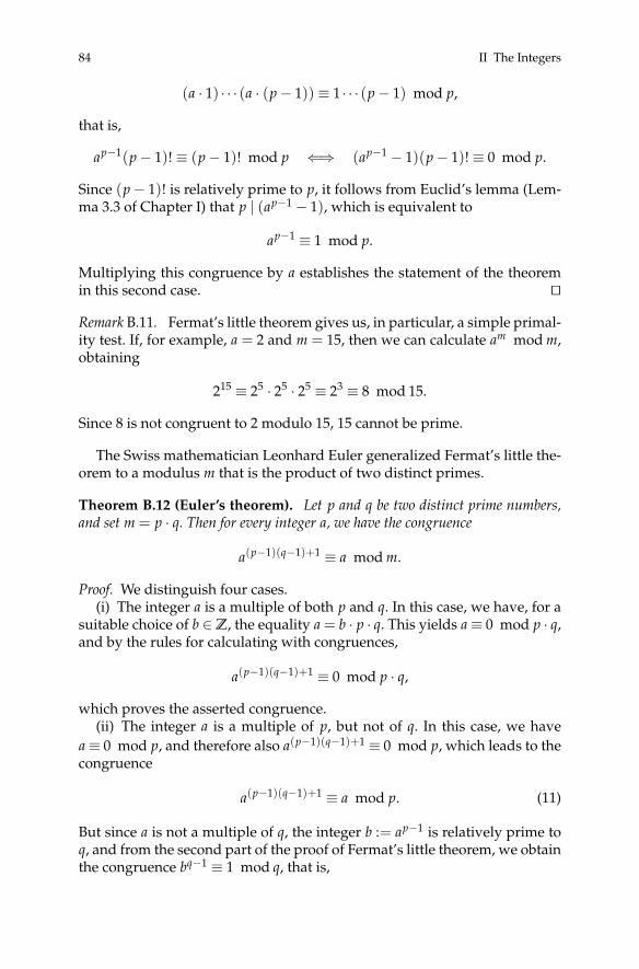
84 II The Integers
(a · 1) · · · (a · (p− 1)) ≡ 1 · · · (p− 1) mod p,
that is,
ap−1(p− 1)! ≡ (p− 1)! mod p ⇐⇒ (ap−1 − 1)(p− 1)! ≡ 0 mod p.
Since (p− 1)! is relatively prime to p, it follows from Euclid’s lemma (Lem-ma 3.3 of Chapter I) that p | (ap−1 − 1), which is equivalent to
ap−1 ≡ 1 mod p.
Multiplying this congruence by a establishes the statement of the theoremin this second case. ut
Remark B.11. Fermat’s little theorem gives us, in particular, a simple primal-ity test. If, for example, a = 2 and m = 15, then we can calculate am mod m,obtaining
215 ≡ 25 · 25 · 25 ≡ 23 ≡ 8 mod 15.
Since 8 is not congruent to 2 modulo 15, 15 cannot be prime.
The Swiss mathematician Leonhard Euler generalized Fermat’s little the-orem to a modulus m that is the product of two distinct primes.
Theorem B.12 (Euler’s theorem). Let p and q be two distinct prime numbers,and set m = p · q. Then for every integer a, we have the congruence
a(p−1)(q−1)+1 ≡ a mod m.
Proof. We distinguish four cases.(i) The integer a is a multiple of both p and q. In this case, we have, for a
suitable choice of b ∈Z, the equality a = b · p · q. This yields a≡ 0 mod p · q,and by the rules for calculating with congruences,
a(p−1)(q−1)+1 ≡ 0 mod p · q,
which proves the asserted congruence.(ii) The integer a is a multiple of p, but not of q. In this case, we have
a≡ 0 mod p, and therefore also a(p−1)(q−1)+1 ≡ 0 mod p, which leads to thecongruence
a(p−1)(q−1)+1 ≡ a mod p. (11)
But since a is not a multiple of q, the integer b := ap−1 is relatively prime toq, and from the second part of the proof of Fermat’s little theorem, we obtainthe congruence bq−1 ≡ 1 mod q, that is,

B. RSA Encryption: An Application of Number Theory 85
a(p−1)(q−1) ≡ 1 mod q .
On multiplication by a, we obtain the congruence
a(p−1)(q−1)+1 ≡ a mod q. (12)
Since the prime numbers p and q are distinct, the two congruences (11) and(12) together yield the asserted congruence
a(p−1)(q−1)+1 ≡ a mod p · q.
(iii) (The integer a is a multiple of q, but not of p. This case can be reducedto the previous case by interchanging the roles of p and q.
(iv) The integer a is a multiple of neither p nor q. As in case (ii), oneproves the congruence
a(p−1)(q−1)+1 ≡ a mod q. (13)
Analogously, one proves the further congruence
a(p−1)(q−1)+1 ≡ a mod p. (14)
Since the two primes p and q are distinct, we obtain from the congruences(13) and (14) the congruence
a(p−1)(q−1)+1 ≡ a mod p · q.
This completes the proof. ut
Remark B.13. The theorems of Fermat and Euler presented here are specialcases of a more general result, which derives ultimately from Lagrange’stheorem (Theorem 4.14). Namely, if (G,◦) is a finite group with identity ele-ment e, then every element g ∈ G satisfies the relation g|G| = e.
We now apply this result. We begin with the set
P(m) :={
a | a ∈ {0, . . . ,m− 1}, (a,m) = 1}
.
It is now easy to see that the set P(m) with respect to congruence multipli-cation is a group with identity element 1, whose order is usually denotedby ϕ(m), called Euler’s ϕ-function. By the previous result, we have for alla ∈ P(m), the relation
aϕ(m) = 1.
We have, therefore, for all a ∈Z with (a,m) = 1, the congruence

86 II The Integers
aϕ(m) ≡ 1 mod m,
from which on multiplication by a, we obtain the congruence aϕ(m)+1 ≡a mod m.
We obtain the connection to the theorems of Euler and Fermat by verify-ing the formulas
ϕ(p) = p− 1 and ϕ(p · q) = (p− 1)(q− 1),
for distinct primes p and q.
B.4 The RSA Cryptosystem
In this section, we shall learn about the ideas behind the RSA cryptosystem.For information on important and interesting questions, in particular secu-rity, including the choice of suitable prime numbers and the private key, aswell as possible attacks against RSA, we refer the reader to the enormousliterature on the subject. We note here that the examples presented in thissection serve a pedagogical purpose and are not of any practical utility.
To send an encrypted message using the RSA algorithm, sender Alice andrecipient Bob proceed as follows:
1. Before a message can be encoded and sent, Bob does the following: Hechooses two distinct “large” prime numbers p and q, of approximatelythree hundred digits, which must be kept secret. Bob then computes theproducts
m = p · q,n = (p− 1) · (q− 1);
note that with the Euler ϕ-function, we have n= ϕ(m). Now Bob choosesa natural number k that is relatively prime to n. The numbers m andk comprise the public key, and recipient Bob sends this information tosender Alice. Bob keeps the numbers p, q, and n private.
2. Alice now begins by transforming the message she wishes to send intoa number a, using, for example, the ASCII code described earlier, withthe properties
(a,m) = 1 and 0 < a < m.
If it turns out that a ≥ m, the message can be split up into several blocksof suitable size so that in each of them, one has a < m. Alice then encryptsher message a by calculating the uniquely determined number b suchthat
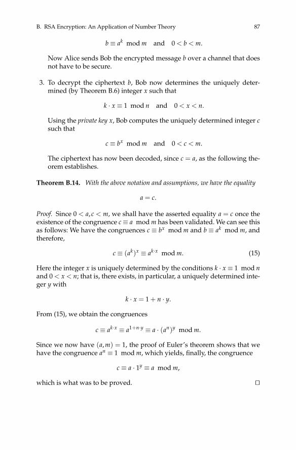
B. RSA Encryption: An Application of Number Theory 87
b ≡ ak mod m and 0 < b < m.
Now Alice sends Bob the encrypted message b over a channel that doesnot have to be secure.
3. To decrypt the ciphertext b, Bob now determines the uniquely deter-mined (by Theorem B.6) integer x such that
k · x ≡ 1 mod n and 0 < x < n.
Using the private key x, Bob computes the uniquely determined integer csuch that
c ≡ bx mod m and 0 < c < m.
The ciphertext has now been decoded, since c = a, as the following the-orem establishes.
Theorem B.14. With the above notation and assumptions, we have the equality
a = c.
Proof. Since 0 < a, c < m, we shall have the asserted equality a = c once theexistence of the congruence c≡ a mod m has been validated. We can see thisas follows: We have the congruences c ≡ bx mod m and b ≡ ak mod m, andtherefore,
c ≡ (ak)x ≡ ak·x mod m. (15)
Here the integer x is uniquely determined by the conditions k · x ≡ 1 mod nand 0 < x < n; that is, there exists, in particular, a uniquely determined inte-ger y with
k · x = 1 + n · y.
From (15), we obtain the congruences
c ≡ ak·x ≡ a1+n·y ≡ a · (an)y mod m.
Since we now have (a,m) = 1, the proof of Euler’s theorem shows that wehave the congruence an ≡ 1 mod m, which yields, finally, the congruence
c ≡ a · 1y ≡ a mod m,
which is what was to be proved. ut

88 II The Integers
Remark B.15. It is possible in the second step of the RSA algorithm to dowithout the requirement (a,m) = 1 in creating the ciphertext. The correct-ness of the RSA algorithm was proved essentially in the previous proof.
Remark B.16. The encryption function used in the RSA algorithm is, in fact,a one-way trapdoor function (see Section B.1). Moreover, the process of en-cryption, which consists essentially in calculating ak mod m, is simple. Thesame holds for calculating bx mod m, provided, of course, that one knowsthe trapdoor, that is, the private key x. One can also easily compute the keyx if like the recipient Bob, one knows the integer ϕ(m) = n = (p− 1)(q− 1).
On the other hand, if one knows the public information m, k, and b, onecould calculate x if one knew the prime decomposition of m, that is, theprime numbers p and q. If m is not particularly large, then one could figureout those prime factors, for example with the SAGE command factor(m).But if m is very large, then deducing the prime decomposition is for all prac-tical purposes impossible using currently known algorithms. Furthermore,if recipient Bob chooses, as is generally done, prime numbers of the same bitlength (balanced RSA algorithm), then it is known that determining the pri-vate key x with only knowledge of the public information m, k, and b is ofthe same level of difficulty as the factorization of m. Thus the security of theRSA cryptosystem rests on the difficulty of the factorization problem.
Recipient Bob
Choice of Prime Numbers p, q:m = p · q,
n = (p − 1)(q − 1),k with (k, n) = 1
Private Key:0 < x < n withk · x ≡ 1 mod n
Public Key:m, k
Coding Messageas a Number:
0 < a < m with(a,m) = 1
Sender Alice
Decoded Ciphertext:0 < c < m withc ≡ bx modm
Ciphertext:0 < b < m withb ≡ ak modm
Public:Transmisson of b
The above diagram provides an overview of the RSA algorithm. The redarrows represent secure communication channels.
Example B.17. To aid in understanding the algorithm, we present here anexample using two small prime numbers.
1. Recipient Bob chooses the prime numbers p = 229 and q = 389. He thencalculates
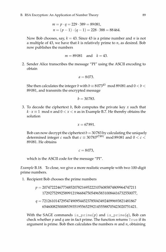
B. RSA Encryption: An Application of Number Theory 89
m = p · q = 229 · 389 = 89081,n = (p− 1) · (q− 1) = 228 · 388 = 88464.
Now Bob chooses, say, k = 43. Since 43 is a prime number and n is nota multiple of 43, we have that k is relatively prime to n, as desired. Bobnow publishes the numbers
m = 89081 and k = 43.
2. Sender Alice transcribes the message “PI” using the ASCII encoding toobtain
a = 8073.
She then calculates the integer b with b≡ 807343 mod 89081 and 0 < b <89081, and transmits the encrypted message
b = 30783.
3. To decode the ciphertext b, Bob computes the private key x such thatk · x ≡ 1 mod n and 0 < x < n as in Example B.7. He thereby obtains thesolution
x = 67891.
Bob can now decrypt the ciphertext b= 30783 by calculating the uniquelydetermined integer c such that c ≡ 3078367891 mod 89081 and 0 < c <89081. He obtains
c = 8073,
which is the ASCII code for the message “PI”.
Example B.18. To close, we give a more realistic example with two 100-digitprime numbers.
1. Recipient Bob chooses the prime numbers
p = 2074722246773485207821695222107608587480996474721117292752992589912196684750549658310084416732550077,
q = 7212610147295474909544523785043492409969382148186765460082500085393519556525921455588705423020751421.
With the SAGE commands is_prime(p) and is_prime(q), Bob cancheck whether p and q are in fact prime. The function returns True if itsargument is prime. Bob then calculates the numbers m and n, obtaining

90 II The Integers
m = p · q= 14964162729898105788684569421835754781481603923778
961041678322180333144368227098607515132513189612225229073721923916059172829814429246504564782903518295622360979392187621542015444916226124162051409417
and
n = (p− 1) · (q− 1)= 14964162729898105788684569421835754781481603923778
961041678322180333144368227098607515132513189612215941741327854955941806610807278145507114404280610412869525486716881905300738973802327334322298107920.
At this point, the reader may wish to test the SAGE command factor(m).Now Bob chooses again, for example, k = 43, since k is relatively primeto n, as desired. One can verify this with the SAGE command gcd(n,k),which returns the greatest common divisor of n and k. One obtainsgcd(n,k) = 1. Bob now publishes the numbers m and k.
2. Sender Alice transcribes the message
PRIME NUMBERS ARE USEFUL!
using the ASCII encoding as
a = 80827377693278857766698283326582693285836970857633.
The SAGE command map(ord,"PRIME"), for example, encodes theword “PRIME” in ASCII as [80,82,73,77,69], giving 8082737769. ThenAlice computes the integer b such that b≡ ak mod m and 0 < b < m andtransmits the encrypted message
b = 3605796078587425125039884757865655248966527926969848103809148617096444525775586803496118061034800457720146085773068579110689354749514665788925986872456073152821301324024745350344439303132600913173384.
The relevant SAGE command is power_mod(a,k,m), which returns theinteger b.
3. To decode the message b, recipient Bob determines the secret key xsuch that k · x ≡ 1 mod n and 0 < x < n. This is accomplished withthe SAGE command k.inverse_mod(n) (see also Remark B.8). Bob ob-tains thereby the solution

B. RSA Encryption: An Application of Number Theory 91
x = 10440113532487050550245048433838898684754607388682996075589527102558007698763092051754743613853217825075633484549969261725542423682427097986793684146799676413130267592026954003935210926047201603331107.
Bob now decodes the message b using the SAGE command
power_mod(b, x,m)
to determine the unique integer c such that c≡ bx mod m and 0 < c < m.Bob thereby obtains the number
c = 80827377693278857766698283326582693285836970857633,
that is, the message “PRIME NUMBERS ARE USEFUL!”
Remark B.19. In applications with limited storage space (chip cards, for ex-ample), there is an increased use of asymmetric encryption algorithms thatuse elliptic curves. Instead of the operations + and · on the integers Z, a spe-cial operation of addition of points on a given elliptic curve is defined. Theoperation ak corresponds to k-fold addition of a point to itself. We shall learnabout addition on elliptic curves in Appendix C. Cryptography that uses el-liptic curves is called, not surprisingly, elliptic curve cryptography (ECC). Foran elementary introduction to this topic, we refer the reader to [8].
References
[1] M. W. Baldoni, C. Cilberto, G. M. Placentini Cattaneo: Elementary numbertheory, cryptography and codes. Translated from the 2006 Italian original byD. A. Gewurz. Springer, Berlin, 2009.
[2] F. L. Bauer: Decrypted secrets: methods and maxims of cryptology. Springer, BerlinHeidelberg New York, 4th edition, 2006.
[3] J. Buchmann: Introduction to cryptography. Springer, Berlin Heidelberg NewYork, 2nd edition, 2004.
[4] W. Diffie, M. E. Hellman: New directions in cryptography. IEEE Trans. Informa-tion Theory IT-22 (1976), 644–654.
[5] D. Kahn: The codebreakers. The comprehensive history of secret communication fromancient times to the internet. Simon & Schuster, 2nd edition, 1997.
[6] R. L. Rivest, A. Shamir, L. Adleman: A method for obtaining digital signatures andpublic-key cryptosystems. Comm. ACM 21 (1978), 120–126.
[7] S. Singh: The code book: the science of secrecy from ancient Egypt to quantum cryp-tography. Random House, 2011.
[8] L. Washington: Elliptic curves: number theory and cryptography. CRC Press, 2ndedition, 2008.

III The Rational Numbers
1. The Integers and Divisibility Theory
In the last section of Chapter II, we introduced the (additive) group of in-tegers (Z, +), which we constructed with the help of Theorem 6.5 of thatchapter from the (additive) semigroup (N, +) of natural numbers. We nowrecall that the natural numbers also have the structure of a monoid withrespect to the multiplication defined in Chapter I. Our first task is to gen-eralize this multiplicative structure to the set of integers. To this end, wereturn to the definition of Z as a set of equivalence classes (see the proof ofTheorem 6.5 of Chapter II); that is,
Z= {[a, b] | (a, b) ∈N×N}.
We now define the product of two integers [a, b] and [a′, b′] by the formula
[a, b] · [a′, b′] := [aa′ + bb′, ab′ + a′b]. (1)
Here, as in Chapter I, we write aa′+ bb′ and ab′+ a′b as an abbreviated formfor the natural numbers (a · a′) + (b · b′) and (a · b′) + (a′ · b). To establishthat this multiplication operation is well defined, we must prove that theproduct (1) is independent of the choice of representatives (a, b) and (a′, b′).To this end, let (c, d) and (c′, d′) be representatives of the equivalence classes[a, b] and [a′, b′]; that is, we have
a + d = b + c and a′ + d′ = b′ + c′. (2)
We must demonstrate the equivalence class equality
[aa′ + bb′, ab′ + a′b] = [cc′ + dd′, cd′ + c′d].
We therefore define the natural number
n := (a′ + b′)(c + d) = a′c + a′d + b′c + b′d.
We then calculate, keeping in mind the equalities (2),
aa′ + bb′ + cd′ + c′d + n = a′(a + d) + b′(b + c) + c(a′ + d′) + d(b′ + c′)
= a′(b + c) + b′(a + d) + c(b′ + c′) + d(a′ + d′)
= ab′ + a′b + cc′ + dd′ + n.
© Springer International Publishing AG 2017
Springer Undergraduate Mathematics Series, https://doi.org/10.1007/978-3-319-69429-0_3J. Kramer and A.-M. von Pippich, From Natural Numbers to Quaternions,
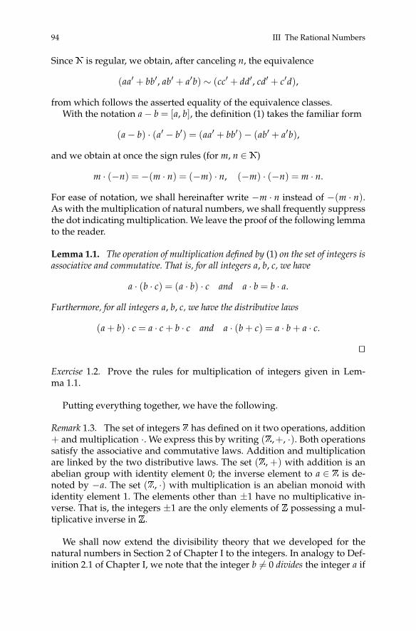
94 III The Rational Numbers
SinceN is regular, we obtain, after canceling n, the equivalence
(aa′ + bb′, ab′ + a′b) ∼ (cc′ + dd′, cd′ + c′d),
from which follows the asserted equality of the equivalence classes.With the notation a− b = [a, b], the definition (1) takes the familiar form
(a− b) · (a′ − b′) = (aa′ + bb′)− (ab′ + a′b),
and we obtain at once the sign rules (for m, n ∈N)
m · (−n) = −(m · n) = (−m) · n, (−m) · (−n) = m · n.
For ease of notation, we shall hereinafter write −m · n instead of −(m · n).As with the multiplication of natural numbers, we shall frequently suppressthe dot indicating multiplication. We leave the proof of the following lemmato the reader.
Lemma 1.1. The operation of multiplication defined by (1) on the set of integers isassociative and commutative. That is, for all integers a, b, c, we have
a · (b · c) = (a · b) · c and a · b = b · a.
Furthermore, for all integers a, b, c, we have the distributive laws
(a + b) · c = a · c + b · c and a · (b + c) = a · b + a · c.
ut
Exercise 1.2. Prove the rules for multiplication of integers given in Lem-ma 1.1.
Putting everything together, we have the following.
Remark 1.3. The set of integers Z has defined on it two operations, addition+ and multiplication ·. We express this by writing (Z,+, ·). Both operationssatisfy the associative and commutative laws. Addition and multiplicationare linked by the two distributive laws. The set (Z, +) with addition is anabelian group with identity element 0; the inverse element to a ∈ Z is de-noted by −a. The set (Z, ·) with multiplication is an abelian monoid withidentity element 1. The elements other than ±1 have no multiplicative in-verse. That is, the integers ±1 are the only elements of Z possessing a mul-tiplicative inverse in Z.
We shall now extend the divisibility theory that we developed for thenatural numbers in Section 2 of Chapter I to the integers. In analogy to Def-inition 2.1 of Chapter I, we note that the integer b 6= 0 divides the integer a if

1. The Integers and Divisibility Theory 95
there exists an integer c such that a = b · c. The notion of a common divisor oftwo integers carries over directly from Definition 2.1 of Chapter I. The va-lidity of the divisibility rules from Lemma 2.4 of Chapter I also carries overdirectly to the integers. By a simple generalization of Remark 2.6 of Chap-ter I, we call the divisors 1,−1, a,−a, or ±1,±a for short, the trivial divisorsof the integer a. Furthermore, we call two integers a, b associates if they differby at most a sign, that is, if a = ±b. A prime number p is now characterizedas an integer greater than 1 that has only the trivial divisors ±1 and ±p.Lemma 2.9 of Chapter I carries over directly to the integers.
In general, one can carry out division with remainder on integers, just aswith the natural numbers.
Theorem 1.4 (Division with remainder, revisited). Let a, b be integers withb 6= 0. Then there exist uniquely determined integers q, r with 0≤ r < |b| such that
a = q · b + r. (3)
Proof. The proof is a simple modification of the proof of Theorem 5.1 ofChapter I and is left to the reader as an exercise. ut
Exercise 1.5. Carry out the proof of Theorem 1.4.
A significant difference between the divisibility theory for the naturalnumbers and that for the integers is the fact that in the integers, it is pos-sible to invoke Euclid’s lemma as an aid in proving the fundamental theo-rem of arithmetic, in contrast to how we proceeded in the case of the naturalnumbers, where Euclid’s lemma appeared only as a consequence of the fun-damental theorem. In this direction, we prove the following lemma.
Lemma 1.6. Let a, b be relatively prime integers, that is, such that a, b have onlythe trivial divisors ±1 in common. Then there exist integers x, y such that
x · a + y · b = 1.
Proof. We consider the set of all integer linear combinations of a and b, thatis, the set
a := {x1 · a + y1 · b | x1, y1 ∈ Z} ⊆ Z.
Since we have either a ∈ a ∩ N or −a ∈ a ∩ N, the intersection a ∩ N isnonempty. By the well-ordering principle (Lemma 1.21 of Chapter I), thereexists a least positive element d ∈ a∩N. We must show that in fact, d = 1.
We note first that since d ∈ a, there exist integers x0 and y0 such that d =x0 · a + y0 · b. Now let c ∈ a be an arbitrary element of the form c = x1 · a +y1 · b with x1, y1 ∈ Z. On dividing c by d with remainder, we obtain q, r ∈ Z,0≤ r < d, so that we have
c = q · d + r. (4)
96 III The Rational Numbers
If we now substitute c = x1 · a + y1 · b and d = x0 · a + y0 · b in (4), we obtain
x1 · a + y1 · b = q(x0 · a + y0 · b) + r,
which is equivalent to
r = (x1 − q · x0)a + (y1 − q · y0)b ∈ a∩N.
If we had r 6= 0, then we would also have 0< r < d. But that would contradictthe minimality of the choice of d ∈ a ∩N. We therefore have r = 0, and sod | c. From the representation c = x1 · a+ y1 · b with the special values x1 = 1,y1 = 0 and x1 = 0, y1 = 1, we have d | a and d | b; that is, d is a common divisorof a and b. But the integers a, b have only the trivial common divisors ±1,and so we must have d = 1. Finally, if we set x := x0 and y := y0, then weobtain
x · a + y · b = d = 1,
as asserted. ut
Lemma 1.7 (Euclid’s lemma, revisited). Let a, b be integers and p a primenumber. If p | a · b, then we must have p | a or p | b.
Proof. We begin with the divisibility relationship p | a · b. If p | a, then we aredone. If, on the other hand, p - a, then we must prove p | b. Since p is primeand p - a, we conclude that a and p are relatively prime. By the previouslemma, there exist, therefore, integers x, y such that
x · a + y · p = 1.
On multiplying this equality by b, we obtain
b = x · ab + yb · p. (5)
The divisibility rules of Lemma 2.4 of Chapter I (extended to the integers)now show us that p divides the right-hand side of (5), whence it also dividesthe left-hand side. That is, we have p | b, as asserted. ut
For the set of integers, the fundamental theorem of arithmetic takes thefollowing form:
Theorem 1.8 (Fundamental theorem of arithmetic, revisited). Every nonzerointeger a can be represented in the form
a = e · pa11 · · · par
r ,
which is the product of e ∈ {±1} and a product of r (r ∈N) powers of the distinctprime numbers p1, . . . , pr with positive natural-number exponents a1, . . . , ar. Thisrepresentation is unique up to the order of the factors.

2. Rings and Subrings 97
Proof. For the absolute value |a| of a, we have
a = e · |a|
with uniquely determined sign e ∈ {±1}. The existence and uniqueness ofthe prime decomposition of the natural number |a| can be inferred from theproof of Theorem 3.1 of Chapter I.
As an alternative to the uniqueness proof there, one can in the presentsituation complete the proof quickly and elegantly using induction and Eu-clid’s lemma. We leave this as an exercise for the reader. ut
Exercise 1.9. Carry out the uniqueness proof of the fundamental theorem ofarithmetic using Lemma 1.7.
If a, b are integers, then the definition of the greatest common divisor (a, b)of a and b can be reduced to Definition 4.1 of Chapter I of the greatest com-mon divisor of natural numbers by setting
(a, b) := (|a|, |b|).
Likewise, the definition of the least common multiple [a, b] of a and b can be re-duced to Definition 4.7 of Chapter I of the least common multiple of naturalnumbers by setting
[a, b] := [|a|, |b|].By carrying over the divisibility criterion given in Lemma 3.5 of Chapter Ito the integers, we obtain at once the analogues of Theorems 4.3 and 4.9of Chapter I for calculating the greatest common divisor and least commonmultiple of integers a and b using prime decompositions.
2. Rings and Subrings
The example presented in the previous section of the integers with the twooperations addition and multiplication that are linked by the distributivelaws is the prototype for the following definition of a ring.
Definition 2.1. A nonempty set R with two operations (generally calledaddition + and multiplication ·) that satisfies the following properties iscalled a ring:(i) (R, +) is an abelian group.(ii) (R, ·) is a semigroup.(iii) For all a, b, c ∈ R, we have the two distributive laws
(a + b) · c = a · c + b · c,a · (b + c) = a · b + a · c.

98 III The Rational Numbers
Definition 2.2. A ring (R,+, ·) is said to be commutative if for all a, b ∈ R,we have the equality a · b = b · a.
Remark 2.3. (i) We call the identity element of the additive group (R, +) ofa ring (R,+, ·) the zero element and denote it by 0. We denote the additiveinverse of a ∈ R by −a. We define the difference of elements a, b ∈ R by a−b := a + (−b).
(ii) The ring (R,+, ·) consisting solely of the zero element 0 is called thezero ring or null ring and is denoted by ({0},+, ·).
(iii) If the multiplicative semigroup (R, ·) in a ring (R,+, ·) that is not thezero ring is a monoid, we call its identity element the unit element and denoteit by 1. The unit element is uniquely determined and necessarily satisfies theinequality 1 6= 0, since we have R 6= {0}.
(iv) To simplify notation, we will, as usual, agree that multiplication takesprecedence over addition (and therefore, a · b + c means (a · b) + c).
Example 2.4. (i) (Z,+, ·) is a commutative ring with unit element.(ii) (Rn,⊕,�) is a commutative ring with unit element.(iii) (2 ·Z,+, ·) is a commutative ring, but it does not have a unit element,
since 1 /∈ 2 ·Z.(iv) The following example is well known from linear algebra. We con-
sider the set of 2× 2 matrices with integer entries, that is, the set
M2(Z) :={
A =
(a bc d
) ∣∣∣∣ a, b, c, d ∈ Z}
.
Two matrices A =(
a bc d
)and A′ =
(a′ b′c′ d′
)are added and multiplied as fol-
lows:
A + A′ =(
a bc d
)+
(a′ b′
c′ d′
):=(
a + a′ b + b′
c + c′ d + d′
)and
A · A′ =(
a bc d
)·(
a′ b′
c′ d′
):=(
aa′ + bc′ ab′ + bd′
ca′ + dc′ cb′ + dd′
),
where the addition and multiplication of the individual entries are the usualoperations on integers. We leave it to the reader as an exercise to showthat (M2(Z),+, ·) is a ring with unit element. The zero and unit elementsof M2(Z) are given by the matrices(
0 00 0
)and
(1 00 1
);
the additive inverse of the matrix A is

2. Rings and Subrings 99
−A :=(−a −b−c −d
).
We note that this ring is not commutative.(v) Let (R,+, ·) be a ring. We define the polynomial ring (R[X],+, ·) in the
variable X with coefficients in R as the set
R[X] :={
∑j∈N
aj · X j∣∣∣∣ aj ∈ R, aj = 0 for all but finitely many j ∈N
}with the operations(
∑j∈N
aj · X j)+
(∑j∈N
bj · X j)
:= ∑j∈N
(aj + bj) · X j,
(∑j∈N
aj · X j)·(
∑j∈N
bj · X j)
:= ∑j∈N
(∑
k,`∈Nk+`=j
(ak · b`))· X j.
We leave it as an exercise to the reader to show that (R[X],+, ·) is a ring.We remark that we have denoted the formal variable in the elements of apolynomial ring by the capital letter X to distinguish between the polyno-mial p(X) ∈ R[X] and its value p(x) ∈ R at the element x ∈ R.
Exercise 2.5. Prove that the polynomial ring (R[X],+, ·) from Example 2.4 (v)is a ring and that it is commutative if and only if (R,+, ·) is commutative.
Exercise 2.6. Let A be a nonempty set and (R,+R, ·R) a ring. Prove that theset map(A, R) of all mappings from A to R is a ring when it is equippedwith the two operations
( f , g) 7→ f + g, with ( f + g)(a) := f (a) +R g(a) ( f , g ∈map(A, R), a ∈ A),
( f , g) 7→ f · g, with ( f · g)(a) := f (a) ·R g(a) ( f , g ∈map(A, R), a ∈ A).
Exercise 2.7. Determine which of the ring properties from Definition 2.1 aresatisfied by the set N with the operations “max” as the addition and + asthe multiplication.
Lemma 2.8. Let (R,+, ·) be a ring. Then for a, b, c ∈ R, we have the following:(i) a · 0 = 0 · a = 0.(ii) a · (−b) = (−a) · b = −a · b.(iii) (−a) · (−b) = a · b.(iv) (a− b) · c = a · c− b · c.(v) a · (b− c) = a · b− a · c.

100 III The Rational Numbers
Proof. (i) By the distributive law, we have a · a = a · (a + 0) = a · a + a · 0, andit therefore follows by adding −a · a to both sides that a · 0 = 0. The equality0 · a = 0 follows analogously.
(ii) Using (i) and the distributive law, we obtain the equality
a · b + a · (−b) = a(b + (−b)
)= a · 0 = 0,
from which the asserted equality a · (−b) = −a · b follows by addition of−a · b to both sides. The second equality, (−a) · b = −a · b, follows analo-gously.
(iii) Using (ii), we compute
(−a) · (−b) = a ·(− (−b)
)= a · b.
(iv) Using the distributive law and (ii), we calculate
(a− b) · c =(a + (−b)
)· c = a · c + (−b) · c = a · c− b · c.
(v) The proof of (v) is analogous to that of (iv). ut
Definition 2.9. An element a 6= 0 of a ring (R,+, ·) is called a left zero divisorif there exists b ∈ R, b 6= 0, such that a · b = 0. One defines right zero divi-sors analogously. If the ring is commutative, we may speak simply of zerodivisors.
A ring (R,+, ·) is called a domain if it has no (left or right) zero divisors. Anonnull commutative ring (R,+, ·) without zero divisors is called an integraldomain.
Example 2.10. (i) The ring (Z,+, ·) is an integral domain.(ii) The rings (Rn,⊕,�) are in general not integral domains, since as a
rule, they possess zero divisors. For example, the element 2 ∈ R6 is a zerodivisor, since we have 2� 3 = 0.
(iii) The noncommutative matrix ring M2(Z) also has zero divisors. Thematrix A =
(0 10 0), for example, is both a left and right zero divisor, since(
0 10 0
)·(
0 10 0
)=
(0 00 0
).
Exercise 2.11. Generalize Example 2.10 (ii) as follows: if n > 1 is not prime,then (Rn,⊕,�) has zero divisors.
Exercise 2.12. Show that if (R,+, ·) is an integral domain, then so is the poly-nomial ring (R[X],+, ·).
Exercise 2.13. Does the ring (map(A, R),+, ·) from Exercise 2.6 have zerodivisors?

2. Rings and Subrings 101
Lemma 2.14. Let (R,+, ·) be a domain with unit element 1. If there exists a pos-itive natural number n such that
n · 1 := 1 + · · ·+ 1︸ ︷︷ ︸n times
= 0,
and n is the minimal positive number with this property, then n is prime.
Proof. We proceed with a proof by contradiction. Assume, then, that thenumber n is not prime. Then there exist natural numbers k, ` ∈ N with1 < k, ` < n such that n = k · `. We thereby obtain
n · 1 = (k · `) · 1 = (k · 1) · (` · 1) = 0.
Since (R,+, ·) is without zero divisors, it follows that
k · 1 = 0 or ` · 1 = 0.
But this contradicts the minimality of n. ut
Definition 2.15. Let (R,+, ·) be a domain with unit element 1 and supposethat there exists a positive natural number p, which we take to be minimal,with the property p · 1 = 0. Then by the above lemma, p must be prime, andwe call p the characteristic of the ring R; we write char(R) = p.
If there is no positive natural number n such that n · 1 = 0, we say that Rhas characteristic zero.
Example 2.16. (i) The ring of integers (Z,+, ·) has characteristic zero,since there is no positive natural number n such that n · 1 = 0.
(ii) If p is a prime, then the ring (Rp,⊕,�) is an integral domain. Itscharacteristic can easily be seen to be
char(Rp) = p,
since for all k ∈ {1, . . . , p− 1}, we have k · 1 6= 0, but p · 1 = 0 inRp.
Definition 2.17. Let (R,+, ·) be a ring with unit element 1 and let a ∈ R bean arbitrary element. An element b ∈ R is called a left inverse of a if b · a = 1.Similarly, an element c ∈ R is a right inverse of a if a · c = 1.
An element d ∈ R is called a (multiplicative) inverse of a if it is both a leftand right inverse, that is, if a · d = d · a = 1. If a ∈ R has a multiplicativeinverse, we denote it by a−1 or 1
a or sometimes 1/a.An element a ∈ R that has a multiplicative inverse in R is called a unit.
Example 2.18. In the ring (Z,+, ·), the elements a 6= ±1 do not have a mul-tiplicative inverse. The units of (Z,+, ·) are +1 and −1.
102 III The Rational Numbers
Exercise 2.19. What are the units of the polynomial ring (Z[X],+, ·)?
Exercise 2.20. Show that the units of a ring (R,+, ·) with unit element 1 forma group with respect to the ring operation of multiplication.
Exercise 2.21. Determine the group of units for each of the rings (Rn,⊕,�),n = 5, 8, 10, 12. Which of these groups of units are isomorphic?
Definition 2.22. Let (R,+, ·) be a ring. A subset S ⊆ R is called a subring ofR if the restriction of the operations +, · to S (which for simplicity we againdenote by +, ·) define a ring structure on S, that is, if (S,+, ·) is itself a ring.We express this relationship by writing S ≤ R.
Lemma 2.23 (Subring criterion). Let (R,+, ·) be a ring, and S⊆ R a nonemptysubset. Then we have the equivalence
S ≤ R ⇐⇒ a− b ∈ S, a · b ∈ S ∀a, b ∈ S.
Proof. (i) If S is a subring of R, then clearly the difference a− b and the prod-uct a · b must be in S for all a, b ∈ S.
(ii) Conversely, suppose that a − b ∈ S, a · b ∈ S for all a, b ∈ S. Since Sis nonempty, we have from the subgroup criterion, namely Lemma 2.25 ofChapter II, that (S, +) is an abelian subgroup of the additive group (R, +).Since we also have a · b ∈ S for all a, b ∈ S, it follows that S is closed undermultiplication. Furthermore, S inherits the associative law with respect tomultiplication and the distributive laws from R. Therefore, (S,+, ·) is a ring,and thus the proof is complete. ut
Example 2.24. The ring (2Z,+, ·) of even integers is a subring of the ring(Z,+, ·) of integers.
Exercise 2.25. Find additional examples of subrings of the ring (Z,+, ·) ofintegers.
Exercise 2.26. Let (R,+, ·) be a ring. Is (R,+, ·) a subring of the ring of poly-nomials (R[X],+, ·)?
3. Ring Homomorphisms, Ideals, and Quotient Rings
In the previous section, we defined for rings the subsidiary object of a sub-ring in analogy to the definition of a subgroup of a group, introduced inChapter II. In pursuit of further structural analysis of groups, we also in-troduced in Chapter II the notions of group homomorphism, normal sub-group, and quotient group. Continuing in that vein in our discussion of

3. Ring Homomorphisms, Ideals, and Quotient Rings 103
rings, we shall now introduce analogous definitions adapted to the morecomplex structure of a ring. We begin with the concept of a ring homomor-phism.
Definition 3.1. Let (R,+R, ·R) and (S,+S, ·S) be rings. A mapping
f : (R,+R, ·R) −→ (S,+S, ·S)
is called a ring homomorphism if for all r1, r2 ∈ R, we have the equalities
f (r1 +R r2) = f (r1) +S f (r2),f (r1 ·R r2) = f (r1) ·S f (r2).
For two rings to be related by a ring homomorphism thus means that theimages under f of the sum and product of r1 and r2 in R are equal to thecorresponding sum and product of the images of r1 and r2 in S. One saysthat the mapping f preserves the ring structure.
A bijective (that is, injective and surjective) ring homomorphism is calleda ring isomorphism. If f : (R,+R, ·R)−→ (S,+S, ·S) is a ring isomorphism, wesay that the rings R and S are isomorphic and write R ∼= S.
Exercise 3.2. Determine which of the following mappings are ring homo-morphisms. Let (R,+, ·) be a nonnull ring, and A a nonempty set:
(a) f1 : R[X] −→ R, where f1
(∑j∈N aj · X j
):= a0.
(b) f2 : R[X] −→ R, where f2
(∑j∈N aj · X j
):= a1.
(c) f3 : map(A, R)−→ R, where f3(g) := r (g ∈map(A, R)) for a fixed r ∈ R.
(d) f4 : map(A, R) −→ R, where f4(g) := g(a) (g ∈ map(A, R)) for a fixeda ∈ A.
(e) f5 : R[X] −→ R, where f5
(∑j∈N aj · X j
):= ∑j∈N aj · rj for a fixed r ∈ R.
In analogy to group homomorphisms introduced in Chapter II, we definethe kernel and image of a ring homomorphism.
Definition 3.3. Let (R,+R, ·R) be a ring with zero element 0R, and let(S,+S, ·S) be a ring with zero element 0S. Furthermore, let f : (R,+R, ·R)−→(S,+S, ·S) be a ring homomorphism. Then
ker( f ) := {r ∈ R | f (r) = 0S}
is called the kernel of f , and

104 III The Rational Numbers
im( f ) := {s ∈ S | ∃r ∈ R : s = f (r)}
is called the image of f .
Lemma 3.4. Let f : (R,+R, ·R) −→ (S,+S, ·S) be a ring homomorphism. Thenker( f ) is a subring of R, and im( f ) is a subring of S.
Proof. The proof proceeds along the same lines as that of Lemma 3.10 ofChapter II and can therefore be left to the reader as an exercise. ut
Exercise 3.5. Prove Lemma 3.4.
Exercise 3.6. Determine the kernel and image of those mappings in Exer-cise 3.2 that are ring homomorphisms.
Remark 3.7. For ease of notation, we shall usually omit the subscripts on theoperations +R and ·R and on the zero element 0R.
Example 3.8. We build here on Example 7.8 of Chapter II, in which we intro-duced the group homomorphism f : (Z, +)−→ (Rn,⊕) via the assignmenta 7→ Rn (a). It is easily verified that this mapping induces a surjective ringhomomorphism
f : (Z,+, ·) −→ (Rn,⊕,�).For the kernel, we have, as in Example 7.8 of Chapter II,
ker( f ) = nZ.
Remark 3.9. The kernel ker( f ) of a ring homomorphism f : (R,+, ·) −→(S,+, ·) is, by Lemma 3.4, a subring of R. We also note that the productsr · a and a · r are in the kernel of f not only for all a, r ∈ ker( f ), but for alla ∈ ker( f ) and r ∈ R, since we have
f (r · a) = f (r) · f (a) = f (r) · 0 = 0,f (a · r) = f (a) · f (r) = 0 · f (r) = 0.
This observation leads to the following definition.
Definition 3.10. Let (R,+, ·) be a ring. A subgroup (a, +) of the additivegroup (R, +) is called an ideal of R if the products
r · a and a · r
are in a for all a ∈ a and all r ∈ R, that is, if we have the inclusions
R · a := {r · a | r ∈ R, a ∈ a} ⊆ a,a · R := {a · r | r ∈ R, a ∈ a} ⊆ a.

3. Ring Homomorphisms, Ideals, and Quotient Rings 105
Remark 3.11. An ideal a of a ring (R,+, ·) is automatically also a subringof R. The converse of this statement is, however, not in general true.
Example 3.12. (i) Let (R,+, ·) be a ring. The subgroup (a, +) = ({0}, +)is clearly an ideal of R. We call it the zero ideal of R and denote it by (0).
(ii) Again, let (R,+, ·) be a ring. The additive group (a, +) = (R, +) is anideal of R. If R has a unit element 1, then this ideal is also called the unit idealof R and is denoted by (1).
(iii) Let (R,+, ·) be a commutative ring. For a fixed a ∈ R, we considerthe set
a := {a · r | r ∈ R}.We can see that a is an ideal of R. Since 0 ∈ a, it follows that a is not empty.If in addition, we have a · r1, a · r2 ∈ a, then we also have that the difference
a · r1 − a · r2 = a · (r1 − r2)
is in a. By the subgroup criterion, Lemma 2.25 of Chapter II, it follows that(a, +) is a subgroup of the additive group (R, +). Finally, if we have a · r ∈ aand s ∈ R, then by the associativity and commutativity of multiplication, wehave
s · (a · r) = a · (r · s) ∈ a;
that is, we have R · a⊆ a, and by commutativity, a · R ⊆ a. Therefore, a is anideal of R. We call it the principal ideal generated by a and denote it by (a).
Exercise 3.13. Let (R,+, ·) be a ring with unit element 1, and let a⊆ R be anideal of R with 1 ∈ a. Show that we must have a= R.
Exercise 3.14. Is there a subring of (Z,+, ·) that is not an ideal of Z?
Exercise 3.15. Find a subring of the polynomial ring (Z[X],+, ·) that is notan ideal of Z[X].
Exercise 3.16. Give examples of ideals in the polynomial ring (Z[X],+, ·).Are there any ideals in this ring that are not principal ideals?
Lemma 3.17. Let f : (R,+, ·)−→ (S,+, ·) be a ring homomorphism. Then ker( f )is an ideal of R.
Proof. From Lemma 3.10 of Chapter II, we see that(
ker( f ), +)
is an additivesubgroup of (R, +). From Remark 3.9, we derive the inclusions
R · ker( f ) ⊆ ker( f ) and ker( f ) · R ⊆ ker( f ),
which prove that ker( f ) is an ideal as claimed. ut
106 III The Rational Numbers
Exercise 3.18. Which of the kernels of the ring homomorphisms in Exer-cise 3.2 are principal ideals?
Lemma 3.19. In the ring (Z,+, ·), all the ideals are principal, that is, for eachideal a, there exists an integer a such that a= (a).
Proof. If a is the zero ideal, then we have a = (0), and we are done. Other-wise, since a is not the zero ideal, there exists a nonzero integer b ∈ a. Multi-plying b by −1 if necessary, we have a nonzero element in the set a ∩N. Bythe well-ordering principle, there exists a least positive integer a ∈ a.
By the definition of an ideal, we see at once that we must have
(a) ⊆ a.
We now prove the reverse inclusion. To this end, let c ∈ a be an arbitraryelement. On dividing c by a with remainder (see Theorem 1.4), we obtainuniquely determined integers q, r with 0≤ r < a such that
c = q · a + r.
Since we have a, c ∈ a, it follows from the fact that a is an ideal that we mustalso have r = c− q · a as an element of a. If we had r 6= 0, then r would bea nonzero element of a∩N that is smaller than a. But that would contradictthe minimality of a. We must therefore have r = 0, and we have c = q · a,that is, we have c ∈ (a). This completes the proof of the inclusion a ⊆ (a).We have thus completed the proof that a = (a), which is what was to beshown. ut
Definition 3.20. Let (R,+, ·) be a ring, and a an ideal of R. Since the addi-tive group (R, +) is abelian by definition, the additive subgroup (a, +) ofthe ideal is automatically a normal subgroup of (R, +). We may thereforeconsider the quotient group (R/a,⊕). The elements of R/a are given bycosets of the form r + a (r ∈ R). The sum of two cosets r1 + a and r2 + a isgiven by
(r1 + a)⊕ (r2 + a) = (r1 + r2) + a
(see Definition 5.1 of Chapter II). We note that in contrast to Definition 5.1of Chapter II, where we denoted the operation in the quotient group by •,here we have chosen the notation⊕ to account for the additive nature of thisconstruction. Incidentally, the reader will have no difficulty in distinguish-ing the notation ⊕ used here from the same notation used in the example of(Rn,⊕,�).
We define a multiplicative operation � on the quotient group (R/a,⊕)by setting, for two cosets r1 + a and r2 + a (in this case as well, there shouldbe no confusion with (Rn,⊕,�)),
(r1 + a)� (r2 + a) := (r1 · r2) + a. (6)

3. Ring Homomorphisms, Ideals, and Quotient Rings 107
This definition appears to depend on the choice of representatives r1 andr2 for the cosets r1 + a and r2 + a. In the following theorem, we prove inparticular that the multiplicative operation � is, in fact, well defined.
Theorem 3.21. Let (R,+, ·) be a ring, and a an ideal of R. Then the set of cosetsR/a together with the two operations
(r1 + a)⊕ (r2 + a) = (r1 + r2) + a,(r1 + a)� (r2 + a) = (r1 · r2) + a,
forms a ring.
Proof. (i) First, we see from Definition 3.20 that (R/a,⊕) is an abelian groupwith identity element (zero element) a.
(ii) We now show that the multiplicative operation � is well defined. Tothis end, let r1, r′1 and r2, r′2 be representatives of the respective cosets r1 + aand r2 + a. To prove that multiplication � is well defined, we must provethe equality
(r1 · r2) + a= (r′1 · r′2) + a. (7)
We have the equalities
r′1 = r1 + a1 (a1 ∈ a),
r′2 = r2 + a2 (a2 ∈ a),
connecting the representatives r1, r′1 and r2, r′2. From these, we calculate
r′1 · r′2 = (r1 + a1) · (r2 + a2) = r1 · r2 + r1 · a2 + a1 · r2 + a1 · a2.
Because a is an ideal, we see that
r1 · a2 + a1 · r2 + a1 · a2 ∈ a.
Therefore, the product r′1 · r′2 is also a representative of the coset (r1 · r2) + a;that is, we have indeed the asserted equality (7). This proves that the multi-plication � is well defined.
(iii) The associativity of the multiplication� is shown, using definition (6)and the associativity of the multiplication operation · , as follows:
(r1 + a)�((r2 + a)� (r3 + a)
)= (r1 + a)�
((r2 · r3) + a
)=(r1 · (r2 · r3)
)+ a=
((r1 · r2) · r3
)+ a
=((r1 · r2) + a
)� (r3 + a) =
((r1 + a)� (r2 + a)
)� (r3 + a).
(iv) The proof of the distributive laws also derives from definition (6) andthe distributive laws in the ring (R,+, ·); for example, we have

108 III The Rational Numbers
(r1 + a)�((r2 + a)⊕ (r3 + a)
)= (r1 + a)�
((r2 + r3) + a
)=(r1 · (r2 + r3)
)+ a=
((r1 · r2) + (r1 · r3)
)+ a
=((r1 · r2) + a
)⊕((r1 · r3) + a
)= (r1 + a)� (r2 + a)⊕ (r1 + a)� (r3 + a).
We have proved that (R/a,⊕,�) is a ring. ut
Definition 3.22. Let (R,+, ·) be a ring, and a an ideal of R. Then the ring(R/a,⊕,�) is called the quotient ring of R by the ideal a.
Remark 3.23. Let f : (R,+, ·) −→ (S,+, ·) be a ring homomorphism. Then,Lemma 3.17 tells us that ker( f ) is an ideal of R; by Theorem 3.21, we mayconsider the quotient ring (R/ker( f ),⊕,�). We recognize the canonicalgroup homomorphism
π : (R, +) −→ (R/ker( f ),⊕)
from Remark 5.6 of Chapter II, defined by the assignment r 7→ r + ker( f ), asa ring homomorphism, since we have
π(r1 · r2) = (r1 · r2) + ker( f )
=(r1 + ker( f )
)�(r2 + ker( f )
)= π(r1)� π(r2).
We call this the canonical ring homomorphism.
Theorem 3.24 (Homomorphism theorem for rings). Let f : (R,+, ·) −→(S,+, ·) be a ring homomorphism. Then f induces a uniquely determined injec-tive ring homomorphism
f : (R/ker( f ),⊕,�) −→ (S,+, ·)
such that f(r+ker( f )
)= f (r) for all r ∈ R. This result can be illustrated schemat-
ically by saying that the following diagram is commutative:
(R,+, ·)π
��
f
''(R/ker( f ),⊕,�)∃! f // (S,+, ·)
Commutativity of the diagram means that the same result is obtained by executingthe mapping f directly or by first executing π and then the mapping f .
Proof. According the homomorphism theorem for groups, Theorem 5.7 ofChapter II, there exists a uniquely determined injective group homomor-

3. Ring Homomorphisms, Ideals, and Quotient Rings 109
phismf : (R/ker( f ),⊕) −→ (S, +)
such that f(r + ker( f )
)= f (r) for all r ∈ R. It thus remains to show that
f respects the multiplicative structure as well. Using the definition of theoperation�, the definition of f , and the ring homomorphism f , we computethe image under f of the product of the two cosets r1 + ker( f ) and r2 +ker( f ) as
f((
r1 + ker( f ))�(r2 + ker( f )
))= f
((r1 · r2) + ker( f )
)= f (r1 · r2)
= f (r1) · f (r2) = f(r1 + ker( f )
)· f(r2 + ker( f )
).
We have thus shown that f is a ring homomorphism, which completes theproof of the homomorphism theorem for rings. ut
Corollary 3.25. Let f : (R,+, ·)−→ (S,+, ·) be a surjective ring homomorphism.Then f determines a uniquely determined ring isomorphism
f : (R/ker( f ),⊕,�) ∼= (S,+, ·)
such that f(r + ker( f )
)= f (r) for all r ∈ R. ut
Example 3.26. (i) We continue Example 3.8, in which we saw that therearises a surjective ring homomorphism
f : (Z,+, ·) −→ (Rn,⊕,�)
with ker( f ) = nZ. By Corollary 3.25 to the homomorphism theorem forrings, we have the ring isomorphism
(Z/nZ,⊕,�) ∼= (Rn,⊕,�),
given by the assignment a + nZ 7→ Rn(a).(ii) Let (R,+, ·) = (Z,+, ·), and let (S,+, ·) be a domain with unit ele-
ment 1. The assignment
n 7→
n · 1 = 1 + · · ·+ 1︸ ︷︷ ︸
n times
, if n ∈ Z, n ≥ 0,
−((−n) · 1
), if n ∈ Z, n < 0,
defines a ring homomorphism f : (Z,+, ·) −→ (S,+, ·). The kernel of f isequal to the ideal
ker( f ) = {n ∈ Z | n · 1 = 0}.We distinguish two cases:

110 III The Rational Numbers
(a) char(S) = 0: In this case, we have by definition that n · 1 6= 0 for alln ∈ Z \ {0}; that is, ker( f ) = {0}, which implies the injectivity of f . Thusevery ring of characteristic zero contains a subring isomorphic to the ring ofintegers (Z,+, ·); in the sequel, we will identify this subring with the inte-gers (Z,+, ·).(b) char(S) = p: In this case, we have by definition that for the prime num-ber p, we have p · 1 = 0; that is, ker( f ) = pZ. By the homomorphism theoremfor rings, we thus obtain an injective ring homomorphism f : Z/pZ −→ S.Therefore every ring of characteristic p contains (an isomorphic copy of) thequotient ring (Z/pZ,⊕,�) ∼= (Rp,⊕,�) as a subring.
Exercise 3.27. Find a ring homomorphism f : (Z[X],+, ·) −→ (Z,+, ·) suchthat for some a ∈ Z, there exists, as described in Corollary 3.25, a ring iso-morphism
(Z[X]/(X− a),⊕,�) ∼= (Z,+, ·).
Exercise 3.28. Formulate and prove an analogue for rings of the group iso-morphism from Exercise 5.11 of Chapter II.
4. Fields and Skew Fields
The motivation to extend the definition of a ring to define fields and skewfields is again based on the desire to remove restrictions on the solutions tolinear equations. If (R,+, ·) is a commutative ring with unit element 1, thenthe equation
a · x = b (a, b ∈ R) (8)
is solvable in R if a has an inverse in R, in which case the solution is x =a−1 · b. A field is a commutative ring with unit element 1 such that each ofits nonzero elements has a multiplicative inverse in R, with the result that(8) always has a solution in R except for the case a = 0 and b 6= 0.
Definition 4.1. Let (R,+, ·) be a ring with unit element 1. Then we denotethe set of units of R by R×; that is,
R× = {a ∈ R | a has a (multiplicative) inverse in R}.
A ring (R,+, ·) with unit element 1 is called a skew field if
R× = R \ {0}.
A commutative skew field is called a field.

4. Fields and Skew Fields 111
Remark 4.2. (i) Let (R,+, ·) be a ring with unit element 1. Then (R×, ·) is agroup with identity element 1. We call it the multiplicative group of the ring(R,+, ·).
(ii) If (R,+, ·) is a skew field, then every a ∈ R, a 6= 0, has a multiplica-tive inverse a−1 = 1
a = 1/a ∈ R. The multiplicative group of the skew field(R,+, ·) is equal to (R \ {0}, ·).
(iii) If (R,+, ·) is a field and a, b ∈ R with b 6= 0, then we use the notation
a · b−1 =ab= a/b.
Example 4.3. Let p be a prime number. Then the ring (Rp,⊕,�) is a skewfield; it is, in fact, a field. The situation is especially simple for the case p = 2,for which have the field comprising the two elements 0, 1.
Exercise 4.4. Try to find a skew field with finitely many elements that is nota field.
Remark 4.5. In Chapter VI, we shall discuss an example of a skew field thatis not a field, namely the Hamiltonian quaternions.
Lemma 4.6. Let (K,+, ·) be a field. Then for a, b, c, d ∈ K, we have the followingcalculational rules:(i) If b, c 6= 0, then
ab=
a · cb · c .
(ii) If b, d 6= 0, thenab± c
d=
a · d± b · cb · d .
(iii) If b, d 6= 0, thenab· c
d=
a · cb · d .
Proof. (i) For b, c 6= 0, we compute
ab= a · b−1 = a · c · c−1 · b−1 = (a · c) · (b · c)−1 =
a · cb · c .
(ii) Using the commutativity of multiplication and the distributive laws,we can calculate, for b, d 6= 0,
ab± c
d= a · b−1 ± c · d−1
= (a · d) · (b · d)−1 ± (b · c) · (b · d)−1
= (a · d± b · c) · (b · d)−1
=a · d± b · c
b · d .

112 III The Rational Numbers
(iii) Using the commutativity of multiplication, we can calculate, for b,d 6= 0,
ab· c
d= (a · b−1) · (c · d−1) = (a · c) · (b · d)−1 =
a · cb · d .
This completes the proof of the lemma. ut
5. Construction of Fields from Integral Domains
In analogy to how we proceeded in Theorem 6.5 of Chapter II, in which weextended regular abelian semigroups to abelian groups, we would like inthis section to embed integral domains in fields.
Remark 5.1. We recall from Definition 2.9 that an integral domain (R,+, ·) isa nonnull commutative ring without zero divisors. This means in particularthat nonzero elements a, b ∈ R satisfy a · b 6= 0.
Furthermore, we observe that for an integral domain (R,+, ·), we havethat (R \ {0}, ·) is a regular abelian semigroup. (Note that since R 6= {0}, itfollows that R \ {0} is nonempty.) Since there are no zero divisors, it followsthat R \ {0} is closed with respect to multiplication. The commutativity ofmultiplication is obvious. If for a, b, c ∈ R \ {0}, we have the equality a · c =b · c, we can transform this in (R,+, ·) to
(a− b) · c = 0.
Since c 6= 0, it follows that a− b = 0, which means that we must have a = b.That is, we can “cancel” the c. This proves the regularity of the semigroup(R \ {0}, ·).
Theorem 5.2. For every integral domain (R,+, ·), there exists a uniquely deter-mined field (K,⊕,�) satisfying the following properties:(i) R is a subset of K, and the restrictions of ⊕ and � to R agree with the opera-
tions + and · .(ii) If (K′,⊕′,�′) is another field satisfying (i), then K is a subfield of K′.
Proof. We must prove existence and uniqueness. We begin with the latter.Uniqueness: The proof of uniqueness of the field (K,⊕,�) to be con-
structed proceeds analogously to the proof of uniqueness in Theorem 6.5of Chapter II using property (ii).
Existence: To prove the existence of the field in question, we consider theset
M := R× (R \ {0}) = {(a, b) | a ∈ R, b ∈ R \ {0}}with the relation ∼ defined as follows:
(a, b) ∼ (c, d) ⇐⇒ a · d = b · c (a, c ∈ R; b, d ∈ R \ {0}).

5. Construction of Fields from Integral Domains 113
Although the initial situation here is similar to that in the proof of Theo-rem 6.5 of Chapter II, there is a subtle difference to be considered, namelythat the Cartesian product M has an asymmetry due to the fact that the twofactors are unequal.
We first observe that as in Theorem 6.5 of Chapter II, the relation ∼ is anequivalence relation.
(a) Reflexivity: Since the multiplication is commutative, we have for alla ∈ R, b ∈ R \ {0} the equality a · b = b · a. That is, (a, b)∼ (a, b). The relation∼ is therefore reflexive.
(b) Symmetry: Let (a, b), (c, d) ∈M have the property (a, b)∼ (c, d). Thatis, a · d = b · c. Since the multiplication is commutative, we conclude thatc · b = d · a, which means precisely that (c, d)∼ (a, b). That is,∼ is symmetric.
(c) Transitivity: Let (a, b), (c, d), (e, f ) ∈M be such that (a, b)∼ (c, d) and(c, d) ∼ (e, f ). We then have the equalities
a · d = b · c, c · f = d · e. (9)
If we multiply the left-hand and right-hand sides of the two equalities to-gether, we obtain, taking into account the associativity and commutativityof multiplication, the following equivalent equalities:
(a · d) · (c · f ) = (b · c) · (d · e),a · d · c · f = b · c · d · e,
(a · f ) · (d · c) = (b · e) · (d · c).
If c 6= 0, then since d 6= 0, we have also d · c 6= 0, on account of the absence ofzero divisors in (R,+, ·), and we can cancel (d · c) in the last equality fromthe right and obtain
a · f = b · e,
which implies that (a, b) ∼ (e, f ). If, on the other hand, we have c = 0, thenwe obtain from (9) that a = e = 0, which implies (a, b) = (0, b) ∼ (0, f ) =(e, f ). Therefore, the relation ∼ is transitive.
We denote by [a, b] ⊆ M the equivalence class of the pair (a, b) ∈ M, andby K the set of all such equivalence classes. For brevity, we write
K := M/ ∼ .
Since the ring (R,+, ·) contains at least the zero element 0 and an addi-tional element h 6= 0, it follows that the set M contains at least the two dis-tinct equivalence classes [0, h] and [h, h]. We now define two operations onthe set K of equivalence classes, which we denote by ⊕ and �. If we have[a, b], [a′, b′] ∈ K, then we define
114 III The Rational Numbers
[a, b]⊕ [a′, b′] := [a · b′ + a′ · b, b · b′],[a, b]� [a′, b′] := [a · a′, b · b′].
Since these definitions apparently depend on the choice of representativesa, b and a′, b′ of the equivalence classes [a, b] and [a′, b′], we must prove thatthese operations ⊕ and � are well defined by showing that they are, in fact,independent of this choice. To this end, let (c, d) and (c′, d′) be arbitraryrepresentatives of [a, b] and [a′, b′]. We then must show that
[a · b′ + a′ · b, b · b′] = [c · d′ + c′ · d, d · d′],[a · a′, b · b′] = [c · c′, d · d′].
(d) Proof that ⊕ is well defined: Since (c, d) ∈ [a, b] and (c′, d′) ∈ [a′, b′],we have
a · d = b · c and a′ · d′ = b′ · c′.We therefore compute, using the associativity, commutativity, and distribu-tivity in R,
(a · b′ + a′ · b) · (d · d′) = (a · d) · (b′ · d′) + (a′ · d′) · (b · d)= (b · c) · (b′ · d′) + (b′ · c′) · (b · d) = (b · b′) · (c · d′ + c′ · d),
from which follows the asserted equivalence
(a · b′ + a′ · b, b · b′) ∼ (c · d′ + c′ · d, d · d′).
(e) Proof that � is well defined: Again, since (c, d) ∈ [a, b] and (c′, d′) ∈[a′, b′], we have
a · d = b · c and a′ · d′ = b′ · c′.Multiplying these two equations together yields, with the help of the asso-ciativity and commutativity of R,
(a · d) · (a′ · d′) = (b · c) · (b′ · c′) ⇐⇒ (a · a′) · (d · d′) = (b · b′) · (c · c′),
from which follows the asserted equivalence
(a · a′, b · b′) ∼ (c · c′, d · d′).
In sum, in (K,⊕,�), we have a set containing at least the two distinctelements [0, h], [h, h] and possessing two operations. In the following threesteps, we shall show that (K,⊕,�) is a field. We begin with the proof that(K,⊕) is an abelian group with identity element [0, h].
(1) As we have seen, the set K is nonempty. We leave it to the reader to prove that the operation ⊕ is associative. The commutativity of ⊕ can beseen from the calculation, with [a, b], [a′, b′] ∈ K,

5. Construction of Fields from Integral Domains 115
[a, b]⊕ [a′, b′] = [a · b′ + a′ · b, b · b′] = [a′ · b + a · b′, b′ · b] = [a′, b′]⊕ [a, b],
where we have used the commutativity of + and · .Since h 6= 0, we have the equivalent equalities
a · b = b · a ⇐⇒ (a · b) · h = (b · a) · h ⇐⇒ (a · h) · b = (b · h) · a.
That is, (a · h, b · h)∼ (a, b). We see, then, that [0, h] is the identity element of(K,⊕), since we have, for all [a, b] ∈ K,
[a, b]⊕ [0, h] = [a · h + 0 · b, b · h] = [a · h, b · h] = [a, b].
The additive inverse of the element [a, b] ∈ K is given by [−a, b] ∈ K, sincewe have
[a, b]⊕ [−a, b] = [a · b− a · b, b · b] = [0, b · b] = [0, h],
where we have used the equivalence (0, b · b) ∼ (0, h). We have thereforeproved that (K,⊕) is an abelian group with identity element [0, h].
(2) Our second step is to show that (K \ {[0, h]},�) is an abelian groupwith identity element [h, h].As already mentioned, we have [h, h] 6= [0, h]. That is, [h, h] ∈ K \ {[0, h]},from which we see that K \ {[0, h]} is nonempty. The associativity of theoperation � follows at once from the associativity of · , namely
[a, b]� ([a′, b′]� [a′′, b′′]) = [a, b]� [a′ · a′′, b′ · b′′]= [a · (a′ · a′′), b · (b′ · b′′)]= [(a · a′) · a′′, (b · b′) · b′′]= [a · a′, b · b′]� [a′′, b′′]
= ([a, b]� [a′, b′])� [a′′, b′′].
The proof that � is commutative follows just as easily, using the commuta-tivity of · . Using again the equality of equivalence classes [a · h, b · h] = [a, b],we further compute
[a, b]� [h, h] = [a · h, b · h] = [a, b].
We see, then, that [h, h] is an identity element for K \ {[0, h]}. Finally, todetermine the multiplicative inverse of an element [a, b] ∈ K \ {[0, h]}, weobserve that on account of (a, b) � (0, h), we have also a 6= 0, whence wealso have (b, a) ∈M. We now claim that the multiplicative inverse of [a, b] ∈K \ {[0, h]} is given by the element [b, a], which, by what we have just noted,again lies in K \ {[0, h]}. In fact, we have
[a, b]� [b, a] = [a · b, b · a] = [h, h],
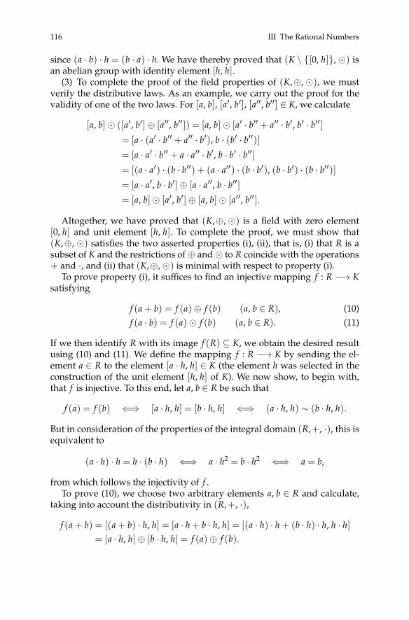
116 III The Rational Numbers
since (a · b) · h = (b · a) · h. We have thereby proved that (K \ {[0, h]},�) isan abelian group with identity element [h, h].
(3) To complete the proof of the field properties of (K,⊕,�), we mustverify the distributive laws. As an example, we carry out the proof for thevalidity of one of the two laws. For [a, b], [a′, b′], [a′′, b′′] ∈ K, we calculate
[a, b]� ([a′, b′]⊕ [a′′, b′′]) = [a, b]� [a′ · b′′ + a′′ · b′, b′ · b′′]= [a · (a′ · b′′ + a′′ · b′), b · (b′ · b′′)]= [a · a′ · b′′ + a · a′′ · b′, b · b′ · b′′]= [(a · a′) · (b · b′′) + (a · a′′) · (b · b′), (b · b′) · (b · b′′)]= [a · a′, b · b′]⊕ [a · a′′, b · b′′]= [a, b]� [a′, b′]⊕ [a, b]� [a′′, b′′].
Altogether, we have proved that (K,⊕,�) is a field with zero element[0, h] and unit element [h, h]. To complete the proof, we must show that(K,⊕,�) satisfies the two asserted properties (i), (ii), that is, (i) that R is asubset of K and the restrictions of⊕ and� to R coincide with the operations+ and ·, and (ii) that (K,⊕,�) is minimal with respect to property (i).
To prove property (i), it suffices to find an injective mapping f : R −→ Ksatisfying
f (a + b) = f (a)⊕ f (b) (a, b ∈ R), (10)f (a · b) = f (a)� f (b) (a, b ∈ R). (11)
If we then identify R with its image f (R) ⊆ K, we obtain the desired resultusing (10) and (11). We define the mapping f : R −→ K by sending the el-ement a ∈ R to the element [a · h, h] ∈ K (the element h was selected in theconstruction of the unit element [h, h] of K). We now show, to begin with,that f is injective. To this end, let a, b ∈ R be such that
f (a) = f (b) ⇐⇒ [a · h, h] = [b · h, h] ⇐⇒ (a · h, h) ∼ (b · h, h).
But in consideration of the properties of the integral domain (R,+, ·), this isequivalent to
(a · h) · h = h · (b · h) ⇐⇒ a · h2 = b · h2 ⇐⇒ a = b,
from which follows the injectivity of f .To prove (10), we choose two arbitrary elements a, b ∈ R and calculate,
taking into account the distributivity in (R,+, ·),
f (a + b) = [(a + b) · h, h] = [a · h + b · h, h] = [(a · h) · h + (b · h) · h, h · h]= [a · h, h]⊕ [b · h, h] = f (a)⊕ f (b).

6. The Rational Numbers 117
To prove (11), we choose two arbitrary elements a, b ∈ R and calculate,taking into account the associativity and commutativity of · ,
f (a · b) = [(a · b) · h, h] = [a · b · h, h] = [a · b · h · h, h · h]= [(a · h) · (b · h), h · h] = [a · h, h]� [b · h, h] = f (a)� f (b).
We have thus proved the structure-preserving properties of f asserted in(10) and (11), and so we see that (K,⊕,�) is indeed a field that satisfiesproperty (i).
To finish the proof, we show, finally, that the field (K,⊕,�) that we haveconstructed is minimal. To do so, we begin with the end of the proof ofTheorem 6.5 of Chapter II and show that if [a · h, h] ∈ K for a ∈ R, a 6= 0,then we have also [h, a · h] ∈ K, and K as a field must necessarily containall elements of the form [a, b] for a ∈ R and b ∈ R \ {0}, which proves theminimality of K. ut
Exercise 5.3. Complete the proof of Theorem 5.2 by proving the associativityof ⊕, the commutativity of �, and the second distributive law.
Definition 5.4. Let (R,+, ·) be an integral domain. The field (K,⊕,�) con-structed in Theorem 5.2 is called the field of fractions of R and is denoted byQuot(R). The elements [a, b] ∈ K are usually represented in the form a · b−1
or ab or a/b.
Exercise 5.5. Show that if (K,+, ·) is a field, then the construction of the fieldof fractions produces nothing new; that is, there exists a ring isomorphism(Quot(K),⊕,�) ∼= (K,+, ·).
6. The Rational Numbers
We would like now to consider in greater depth the field (K,⊕,�) con-structed in Theorem 5.2 from the integral domain (R,+, ·) = (Z,+, ·). Thiswill lead us to the field of rational numbers.
We note first that the equivalence relation ∼ defined on the Cartesianproduct Z× (Z \ {0}) now takes the form
(a, b) ∼ (c, d) ⇐⇒ a · d = b · c (a, b ∈ Z;b, d ∈ Z \ {0}).
The field (K,⊕,�) is given, by the proof of Theorem 5.2, by the set of allequivalence classes a
b = [a, b] of pairs (a, b) ∈ Z× (Z \ {0}) with the opera-tions
ab⊕ a′
b′=
a · b′ + a′ · bb · b′ and
ab� a′
b′=
a · a′b · b′ ,

118 III The Rational Numbers
for ab , a′
b′ ∈K. The zero element of (K,⊕,�) is given by 01 and the unit element
by 11 , where 0 and 1 denote the respective integers zero and one.
We see from the proof of Theorem 5.2 that the set of integers Z stands inbijection to the set { a
1 | a ∈ Z}. This bijection is induced by the assignmenta 7→ [a · 1, 1] = a
1 . Once we have identified the set of integers Z with theset { a
1 | a ∈ Z}, that is, once we set a = a1 , we may then consider Z to be a
subset of K.
Definition 6.1. We shall hereinafter denote the set (K,⊕,�) by (Q,+, ·),and we shall call it the field of rational numbers. We may represent Q as a setin the form
Q=
{ab
∣∣∣∣ a ∈ Z, b ∈ Z \ {0}}
.
We call the rational number ab a fraction or the quotient of the integers a and b.
Remark 6.2. (i) For fractions ab and a′
b′ , we can rediscover the well-knownoperations of addition, subtraction, and multiplication, namely
ab± a′
b′=
a · b′ ± a′ · bb · b′ and
ab· a′
b′=
a · a′b · b′ .
If ab 6= 0, then we have the familiar rule( a
b
)−1=
ba
.
(ii) The zero element 0 and unit element 1 of the integers Z are also, bythe identification made above, equal to the zero and unit elements of therational numbersQ.
(iii) In considering the quotient ab , one should always keep in mind the
underlying equivalence class, namely
35=
610
=915
= · · · .
That is, each of the pairs (3, 5), (6, 10), (9, 15), . . . is a representative of therational number 3
5 .Of course, behind this is lurking the fact that by construction, we have
ab=
cd⇐⇒ a · d = b · c.
Exercise 6.3. Show that every rational number r has exactly one represen-tation (a, b) ∈ Z × (Z \ {0}) such that a and b are relatively prime andb ∈N \ {0}.
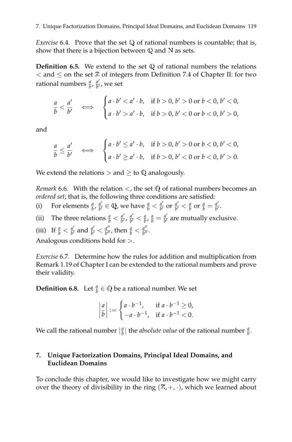
7. Unique Factorization Domains, Principal Ideal Domains, and Euclidean Domains 119
Exercise 6.4. Prove that the set Q of rational numbers is countable; that is,show that there is a bijection betweenQ andN as sets.
Definition 6.5. We extend to the set Q of rational numbers the relations< and ≤ on the set Z of integers from Definition 7.4 of Chapter II: for tworational numbers a
b , a′b′ , we set
ab<
a′
b′⇐⇒
a · b′ < a′ · b, if b > 0, b′ > 0 or b < 0, b′ < 0,
a · b′ > a′ · b, if b > 0, b′ < 0 or b < 0, b′ > 0,
and
ab≤ a′
b′⇐⇒
a · b′ ≤ a′ · b, if b > 0, b′ > 0 or b < 0, b′ < 0,
a · b′ ≥ a′ · b, if b > 0, b′ < 0 or b < 0, b′ > 0.
We extend the relations > and ≥ toQ analogously.
Remark 6.6. With the relation <, the set Q of rational numbers becomes anordered set; that is, the following three conditions are satisfied:(i) For elements a
b , a′b′ ∈Q, we have a
b < a′b′ or a′
b′ <ab or a
b = a′b′ .
(ii) The three relations ab < a′
b′ ,a′b′ <
ab , a
b = a′b′ are mutually exclusive.
(iii) If ab < a′
b′ and a′b′ <
a′′b′′ , then a
b < a′′b′′ .
Analogous conditions hold for >.
Exercise 6.7. Determine how the rules for addition and multiplication fromRemark 1.19 of Chapter I can be extended to the rational numbers and provetheir validity.
Definition 6.8. Let ab ∈Q be a rational number. We set∣∣∣∣ ab∣∣∣∣ :=
{a · b−1, if a · b−1 ≥ 0,−a · b−1, if a · b−1 < 0.
We call the rational number | ab | the absolute value of the rational number ab .
7. Unique Factorization Domains, Principal Ideal Domains, andEuclidean Domains
To conclude this chapter, we would like to investigate how we might carryover the theory of divisibility in the ring (Z,+, ·), which we learned about
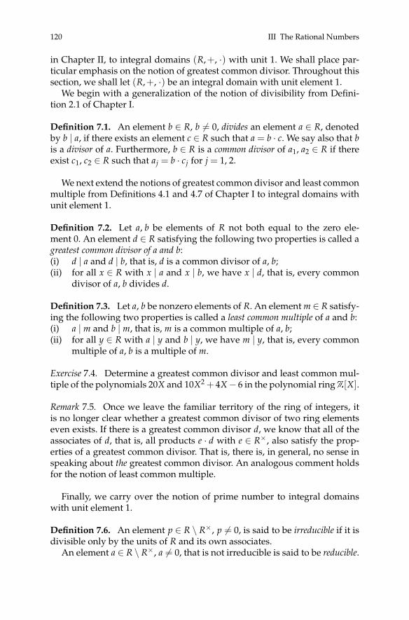
120 III The Rational Numbers
in Chapter II, to integral domains (R,+, ·) with unit 1. We shall place par-ticular emphasis on the notion of greatest common divisor. Throughout thissection, we shall let (R,+, ·) be an integral domain with unit element 1.
We begin with a generalization of the notion of divisibility from Defini-tion 2.1 of Chapter I.
Definition 7.1. An element b ∈ R, b 6= 0, divides an element a ∈ R, denotedby b | a, if there exists an element c ∈ R such that a = b · c. We say also that bis a divisor of a. Furthermore, b ∈ R is a common divisor of a1, a2 ∈ R if thereexist c1, c2 ∈ R such that aj = b · cj for j = 1, 2.
We next extend the notions of greatest common divisor and least commonmultiple from Definitions 4.1 and 4.7 of Chapter I to integral domains withunit element 1.
Definition 7.2. Let a, b be elements of R not both equal to the zero ele-ment 0. An element d ∈ R satisfying the following two properties is called agreatest common divisor of a and b:(i) d | a and d | b, that is, d is a common divisor of a, b;(ii) for all x ∈ R with x | a and x | b, we have x | d, that is, every common
divisor of a, b divides d.
Definition 7.3. Let a, b be nonzero elements of R. An element m ∈ R satisfy-ing the following two properties is called a least common multiple of a and b:(i) a | m and b | m, that is, m is a common multiple of a, b;(ii) for all y ∈ R with a | y and b | y, we have m | y, that is, every common
multiple of a, b is a multiple of m.
Exercise 7.4. Determine a greatest common divisor and least common mul-tiple of the polynomials 20X and 10X2 + 4X− 6 in the polynomial ringZ[X].
Remark 7.5. Once we leave the familiar territory of the ring of integers, itis no longer clear whether a greatest common divisor of two ring elementseven exists. If there is a greatest common divisor d, we know that all of theassociates of d, that is, all products e · d with e ∈ R×, also satisfy the prop-erties of a greatest common divisor. That is, there is, in general, no sense inspeaking about the greatest common divisor. An analogous comment holdsfor the notion of least common multiple.
Finally, we carry over the notion of prime number to integral domainswith unit element 1.
Definition 7.6. An element p ∈ R \ R×, p 6= 0, is said to be irreducible if it isdivisible only by the units of R and its own associates.
An element a ∈ R \ R×, a 6= 0, that is not irreducible is said to be reducible.
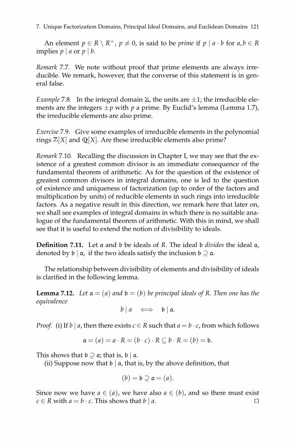
7. Unique Factorization Domains, Principal Ideal Domains, and Euclidean Domains 121
An element p ∈ R \ R×, p 6= 0, is said to be prime if p | a · b for a,b ∈ Rimplies p | a or p | b.
Remark 7.7. We note without proof that prime elements are always irre-ducible. We remark, however, that the converse of this statement is in gen-eral false.
Example 7.8. In the integral domain Z, the units are ±1; the irreducible ele-ments are the integers ±p with p a prime. By Euclid’s lemma (Lemma 1.7),the irreducible elements are also prime.
Exercise 7.9. Give some examples of irreducible elements in the polynomialrings Z[X] andQ[X]. Are these irreducible elements also prime?
Remark 7.10. Recalling the discussion in Chapter I, we may see that the ex-istence of a greatest common divisor is an immediate consequence of thefundamental theorem of arithmetic. As for the question of the existence ofgreatest common divisors in integral domains, one is led to the questionof existence and uniqueness of factorization (up to order of the factors andmultiplication by units) of reducible elements in such rings into irreduciblefactors. As a negative result in this direction, we remark here that later on,we shall see examples of integral domains in which there is no suitable ana-logue of the fundamental theorem of arithmetic. With this in mind, we shallsee that it is useful to extend the notion of divisibility to ideals.
Definition 7.11. Let a and b be ideals of R. The ideal b divides the ideal a,denoted by b | a, if the two ideals satisfy the inclusion b⊇ a.
The relationship between divisibility of elements and divisibility of idealsis clarified in the following lemma.
Lemma 7.12. Let a = (a) and b = (b) be principal ideals of R. Then one has theequivalence
b | a ⇐⇒ b | a.
Proof. (i) If b | a, then there exists c ∈ R such that a = b · c, from which follows
a= (a) = a · R = (b · c) · R ⊆ b · R = (b) = b.
This shows that b⊇ a; that is, b | a.(ii) Suppose now that b | a, that is, by the above definition, that
(b) = b⊇ a= (a).
Since now we have a ∈ (a), we have also a ∈ (b), and so there must existc ∈ R with a = b · c. This shows that b | a. ut

122 III The Rational Numbers
Definition 7.13. Let a and b be ideals of R. Then we call the set
a+ b := {a + b | a ∈ a, b ∈ b}
the sum of the ideals a and b.
Lemma 7.14. Let a and b be ideals of R. Then we have the following:(i) The sum a+ b of the ideals a and b is an ideal of R. It is the smallest ideal of
R containing a and b.(ii) The intersection a ∩ b of the ideals a and b is an ideal of R. It is the largest
ideal of R that is contained in the ideals a and b.
Proof. (i) Using the subgroup criterion, Lemma 2.25 of Chapter II, it is easyto verify that (a+ b, +) is a subgroup of (R, +). For r ∈ R and a + b ∈ a+ b,we obtain
r(a + b) = r · a + r · b ∈ a+ b.
This proves that a+ b is an ideal of R. Since an ideal is a group under ad-dition, it must contain all sums of its elements, and so an ideal containingboth a and b must contain all sums of the form a + b (with a ∈ a and b ∈ b).This shows that a+ b is the smallest ideal containing both a and b.
(ii) We leave this part of the proof as an exercise for the reader. ut
Exercise 7.15. Carry out part (ii) of the proof of Lemma 7.14.
Remark 7.16. We point out here that the union of two ideals is not, in gen-eral, an ideal. For example, the union of the ideals a= 2Z and b= 3Z is noteven closed under addition, since we have 2 + 3 = 5 /∈ 2Z∪ 3Z.
Lemma 7.14 together with Definition 7.11 motivates the following defini-tion.
Definition 7.17. Let a and b be ideals of R. Then the ideal a+ b, the sum ofthose ideals, is the greatest common divisor of the ideals a and b, for which wewrite (a, b).
The intersection ideal a∩ b is called the least common multiple of the idealsa and b, for which we write [a, b].
We now consider three types of integral domain (R,+, ·) with unit ele-ment 1 for which the greatest common divisor of two elements exists. Ineach case, we will show how to calculate the greatest common divisor. Weshall denote the greatest common divisor of a, b ∈ R by (a, b), as usual. Wemust keep in mind, however, that (a, b) is defined only up to multiplicationby a unit in R. In contrast, the principal ideal
((a, b)
)generated by (a, b) in
R is uniquely determined.

7. Unique Factorization Domains, Principal Ideal Domains, and Euclidean Domains 123
7.1 Unique Factorization Domains
Definition 7.18. An integral domain (R,+, ·) with unit element 1 is called aunique factorization domain (that is, a ring with unique prime decomposition)if every nonzero, nonunit element (that is, every a in R \ R×, a 6= 0) canbe represented uniquely (up to order and multiplication by a unit) as theproduct of powers of irreducible elements. Unique factorization domainsare also sometimes called factorial rings.
Example 7.19. (i) The ring (Z,+, ·) is a unique factorization domain byTheorem 1.8.
(ii) The set Q[X] of polynomials in the variable X with rational coeffi-cients and with the usual addition and multiplication of polynomials, thatis, (Q[X],+, ·), is an integral domain with unit element 1. It can be shownthat (Q[X],+, ·) is a unique factorization domain.
Lemma 7.20. Let (R,+, ·) be a unique factorization domain. Furthermore, let a, bbe elements of R not both equal to the zero element 0 with the unique (up to orderand multiplication by units) prime-power decompositions
a = ∏p∈R
p irreducible
pap , b = ∏p∈R
p irreducible
pbp
into irreducible elements. Then a greatest common divisor (a, b) of a and b is
(a, b) = ∏p∈R
p irreducible
pdp ,
where dp := min(ap, bp).
Proof. The proof is completely analogous to the proof of Theorem 4.3 ofChapter I. ut
Remark 7.21. Later, we shall see examples of rings that are not unique fac-torization domains. The following theorem, which we give without proof,suggests why it is not so easy to find integral domains that are not uniquefactorization domains.
Theorem 7.22 (Gauss’s theorem). If (R,+, ·) is a unique factorization domain,then the polynomial ring (R[X],+, ·) is also a unique factorization domain. ut

124 III The Rational Numbers
7.2 Principal Ideal Domains
Definition 7.23. An integral domain (R,+, ·) with unit element 1 is calleda principal ideal domain if every ideal of R is a principal ideal, that is, if everyideal a of R is generated by some a ∈ R, that is, a= (a).
Example 7.24. (i) The ring (Z,+, ·) is a principal ideal domain by Lem-ma 3.19.
(ii) It can be shown that the polynomial ring (Q[X],+, ·) is also a princi-pal ideal domain. See Example 7.34 below.
Exercise 7.25. We have already seen that (Z[X],+, ·) is not a principal idealdomain. Try to find other such examples.
The following theorem shows the relationship between unique factoriza-tion domains and principal ideal domains. We present it without proof.
Theorem 7.26. Every principal ideal domain is a unique factorization domain. ut
Remark 7.27. The converse is false: (Z[X],+, ·) is a unique factorization do-main by Gauss’s theorem, but it is not a principal ideal domain.
On the other hand, it can be shown that in principal ideal domains, ev-ery irreducible element is also a prime element. Thus in a principal idealdomain, the notions of primality and irreducibility are equivalent.
Lemma 7.28. Let (R,+, ·) be a principal ideal domain. Furthermore, let a, b beelements of R, not both equal to the zero element 0. Then the ideal (a) + (b) is aprincipal ideal. That is, there exists d ∈ R such that
(a) + (b) = (d).
Then d is a greatest common divisor of a and b. That is, d = (a, b).
Proof. We must show that d satisfies the following two properties:(i) d | a and d | b,(ii) for all x ∈ R with x | a and x | b, we have x | d.
Proof of (i): Since by construction, (a) ⊆ (a) + (b) = (d) and (b) ⊆ (a) +(b) = (d), we obtain at once using Lemma 7.12 that d | a and d | b.
Proof of (ii): Let x ∈ R be a common divisor of a and b. Then Lemma 7.12implies that
(a) ⊆ (x) and (b) ⊆ (x).
But then the ideal (d) = (a) + (b) is contained in the principal ideal (x); thatis, (d) ⊆ (x). Another application of Lemma 7.12 shows that x | d. ut

7. Unique Factorization Domains, Principal Ideal Domains, and Euclidean Domains 125
Lemma 7.29. Let (R,+, ·) be a principal ideal domain. Furthermore, let a, b beelements of R, not both equal to the zero element 0. Then there exist x, y ∈ R suchthat a greatest common divisor (a, b) of a, b is given by
(a, b) = x · a + y · b.
Proof. By Lemma 7.28, a greatest common divisor d = (a, b) of a, b is deter-mined by the equation of ideals
(d) = (a) + (b).
That is, we have in particular that d ∈ (a) + (b). Since now the elements ofthe ideal (a) + (b) are given by
(a) + (b) = {a′ + b′ | a′ ∈ (a), b′ ∈ (b)} = {r · a + s · b | r, s ∈ R},
we have that d is of the form
d = x · a + y · b,
with x, y ∈ R. ut
7.3 Euclidean Domains
Definition 7.30. An integral domain (R,+, ·) with unit element 1 is calleda Euclidean domain if there exists a valuation function w : R \ {0} −→Q sat-isfying the following two properties:(i) (Division with remainder). If a, b ∈ R, b 6= 0, then there exist q, r ∈ R such
that a = q · b + r with w(r) < w(b) or r = 0.(ii) For every s ∈Q, the set
W(s) :={
w(a) | a ∈ R \ {0}, w(a) < s}
is finite.
Example 7.31. The ring of integers (Z,+, ·) is a Euclidean domain with thevaluation function w : Z \ {0} −→Q given by the absolute value w(a) := |a|(a ∈ Z \ {0}). The validity of property (i) in Definition 7.30 is an immediateconsequence of Theorem 1.4, on division with remainder of integers. Prop-erty (ii) is satisfied because for a given rational number s, at most finitelymany integers have absolute value less than s.
Theorem 7.32. Every Euclidean domain (R,+, ·) is a principal ideal domain.
Proof. Let (R,+, ·) be a Euclidean domain with valuation function w : R \{0}−→ Q. We must show that every ideal a ⊆ R is principal. If a is the zero
126 III The Rational Numbers
ideal, then a= (0), and we are done. We may therefore assume that a 6= (0).Therefore, a has at least one element a0 6= 0. Let w0 := w(a0)∈Q be the valueof a0 under w. From property (ii) of Definition 7.30, we have that the set{
w(a) | a ∈ a \ {0}, w(a) < w0}
is finite. There exists, therefore, a ∈ a, a 6= 0, with minimal value w(a). Letnow b ∈ a be arbitrary. Using property (i), we divide b by a with remainder,that is, we determine q, r ∈ R such that
b = q · a + r
with r = 0 or w(r) < w(a). If we had r 6= 0, then r = b − q · a would be anonzero element of a with a value w(r) that was strictly less than the valuew(a) of a. This contradicts the choice of a, and so we must have r = 0. Wetherefore have b = q · a, whence a= (a). ut
Remark 7.33. We note that in Definition 7.30, we did not need to requirethe existence of a unit element 1, since the existence is a consequence of theother requirements. Namely, since (R,+, ·) is an integral domain, the ideala = R is nontrivial. That is, there exists a ∈ R, a 6= 0, with minimal valuew(a) ∈Q. If we now divide a with remainder by itself, we obtain, as in theproof above, a = e · a for some e ∈ R. Canceling the a yields the desired unitelement e = 1.
Example 7.34. We show that (Q[X],+, ·) is a Euclidean domain. First of all,(Q[X],+, ·) is an integral domain. If P ∈Q[X] is a nonzero polynomial, wemay map P to its degree deg(P), given as the largest natural number ap-pearing as an exponent in P. We thereby obtain the mapping
deg :Q[X] \ {0} −→N⊆Q.
Division with remainder of polynomials shows that property (i) in Defini-tion 7.30 is satisfied. The validity of property (ii) can be seen from the factthat there are only finitely many possibilities for the degree of a polynomialto be less than a given rational number.
In the previous subsection, we saw in Lemma 7.29 that in principal idealdomains (R,+, ·), one can represent a greatest common divisor d of twoelements a, b ∈ R as a linear combination d = x · a + y · b. However, beyondthe existence of x, y∈ R, we could say nothing about how to determine thoseelements. The following theorem clarifies the issue.
Theorem 7.35 (Euclidean algorithm). Let (R,+, ·) be a Euclidean domain. Weconsider, for a, b ∈ R with b 6= 0, an extended division with remainder that leads tothe following:

7. Unique Factorization Domains, Principal Ideal Domains, and Euclidean Domains 127
a = q1 · b + r1, 0 < w(r1) < w(b) or r1 = 0;b = q2 · r1 + r2, 0 < w(r2) < w(r1) or r2 = 0;
r1 = q3 · r2 + r3, 0 < w(r3) < w(r2) or r3 = 0;· · ·
rn−2 = qn · rn−1 + rn, 0 < w(rn) < w(rn−1) or rn = 0;rn−1 = qn+1 · rn + rn+1, 0 < w(rn+1) < w(rn) or rn+1 = 0;· · ·
This process ends after finitely many steps; that is, there exists n ∈ N such thatrn+1 = 0. Moreover, the last nonvanishing remainder rn is a greatest common divi-sor of a and b.
Proof. Since (R,+, ·) is a Euclidean domain, the set of values
W(w(b)
):={
w(a)∣∣ a ∈ R \ {0}, w(a) < w(b)
}is finite. This has the consequence that the extended division with remaindermust end after finitely many steps, that is, that there exists n ∈N such thatrn+1 = 0. In what follows, rn will denote the last nonvanishing remainder.
We now show that rn = (a, b). For rn, we have to verify the two propertiesof a greatest common divisor from Definition 7.2.
(i) We show first that rn is a common divisor of a and b. If we look at thelast line in the display above, we see that rn | rn−1. From the penultimateline, rn−2 = qn · rn−1 + rn, we conclude that rn | rn−2. Working our way up-ward through successive rows, we obtain rn | b and finally rn | a, and so rn isindeed a common divisor of a and b.
(ii) We show now that rn divides every common divisor x of a and b.From the first row of the above display, we obtain x | r1. We conclude fromthe second row that x | r2. Continuing in this way, we see that x must divideall the successive remainders, that is, we obtain in particular that x | rn, asasserted. ut
Remark 7.36 (Extended Euclidean algorithm). Let (R,+, ·) be a Euclidean do-main, and a, b ∈ R with b 6= 0. An analysis of Theorem 7.35 shows that fromthe data of the extended division with remainder, we can determine explicitelements x, y ∈ R such that
(a, b) = x · a + y · b.
From the penultimate row of the display given in Theorem 7.35, we canread off that rn = rn−2 − qn · rn−1. Using the third row from the end, that is,rn−3 = qn−1 · rn−2 + rn−1, we obtain

128 III The Rational Numbers
rn = rn−2 − qn · rn−1
= rn−2 − qn · (rn−3 − qn−1 · rn−2)
= (−qn) · rn−3 + (1 + qn · qn−1) · rn−2.
We see, then, that by working our way up the display, we can represent rn asa linear combination of two successive remainders rj, rj+1 (j = n− 2, . . . , 1).After n− 2 steps, we obtain
rn = x1 · r1 + x2 · r2
with suitable x1, x2 ∈ R. If in this equation we replace r2 by b− q2 · r1 andthen r1 by a− q1 · b, we obtain the desired x, y ∈ R.
To close the main part of this chapter, we would like to illustrate some ofthe concepts presented by means of an example.
Example 7.37. Consider the Euclidean domain (Z,+, ·) of integers. We wishto compute the greatest common divisor (a, b) for a = 113 and b = 29 andrepresent it as a linear combination of integers. Repeated division with re-mainder yields
113 = 3 · 29 + 26,29 = 1 · 26 + 3,26 = 8 · 3 + 2,3 = 1 · 2 + 1,2 = 2 · 1 + 0,
whence we have (113, 29) = 1. To obtain the desired integer linear combi-nation representing the greatest common divisor, we proceed through thedisplay above from bottom to top. We obtain
1 = 3− 1 · 2,= 3− 1 · (26− 8 · 3) = 9 · 3− 1 · 26,= 9 · (29− 1 · 26)− 1 · 26 = 9 · 29− 10 · 26,= 9 · 29− 10 · (113− 3 · 29) = −10 · 113 + 39 · 29,
and we have(113, 29) = 1 = −10 · 113 + 39 · 29.
Exercise 7.38. Carry out the Euclidean algorithm to determine the greatestcommon divisor (a, b) of a, b in the following two cases:(a) a = 123456789, b = 555555555 in the ring (Z,+, ·).(b) a = X4 + 2X3 + 2X2 + 2X + 1, b = X3 + X2 − X − 1 in the polynomial
ring (Q[X],+, ·).

C. Rational Solutions of Equations: A First Glimpse 129
C. Rational Solutions of Equations: A First Glimpse
We conclude this chapter with a first look at the solution of polynomialequations in rational numbers, which were introduced in Section 6 of thischapter. This will lead us to some classical questions, which in part wereresolved only relatively recently and some of which are topics of active re-search in number theory today.
C.1 The General Problem
In generalizing linear algebra, where one looks for common solutions to sev-eral linear equations in several variables X1, . . . , Xn in a field K (such as thefield of rational numbers Q, the field of real numbers R, and the field of com-plex numbers C, which will be constructed in the following chapters), in thefield of complex algebraic geometry one is interested in understanding themanifold of all common solutions of equations of the form
Pj(X1, . . . , Xn) = 0 (j = 1, . . . ,r),
where Pj = Pj(X1, . . . , Xn) are polynomials of arbitrary degree with coeffi-cients in C; that is, P1, . . . , Pr are elements of the polynomial ring C[X1, . . . , Xn].
In arithmetic algebraic geometry, one is interested in the analogous ques-tion about the field Q of rational numbers. In particular, one is interested inthe following two fundamental questions:
(A) Is there an n-tuple (x1, . . . , xn) of rational numbers such that
Pj(x1, . . . , xn) = 0
for j = 1, . . . ,r?
(B) If the answer to (A) is affirmative, is the number of such n-tuples finiteor infinite?
In what follows, we shall assume that question (A) has been answered inthe affirmative, and we shall investigate question (B) for the case of twovariables X = X1,Y = X2 and r = 1, that is, the case of a polynomial P =P1 ∈Q[X,Y].
Let, therefore, P = P(X,Y) be a polynomial in the two variables X,Y withrational coefficients. To answer the two questions posed above, we may as-sume without loss of generality that the coefficients of P are in fact integers.That is, we may assume that P is an element of the polynomial ring Z[X,Y].In regard to question (A), we are interested in whether there exist rationalnumbers x,y such that P(x,y) = 0. This question can be formulated geomet-rically as follows. The equation
P(X,Y) = 0

130 III The Rational Numbers
defines an algebraic curve C in the X,Y-plane. The question of rational solu-tions x,y of the polynomial equation P(X,Y) = 0 is thereby reduced to thequestion of points on the curve C that have rational coordinates. To studyquestion (A), we write
C(Q) := {(x,y) ∈Q2 |P(x,y) = 0}
and call this the set of rational points on C. For example, for the unit circlewith center at the origin, defined by the equation X2 + Y2 − 1 = 0, we seethat (3/5,4/5) is a rational point.
Beginning with the algebraic curve C defined by the equation P(X,Y) = 0,we may reformulate questions (A) and (B) as follows:
(A) Is the set C(Q) nonempty?
(B) If the answer to (A) is affirmative, is C(Q) finite or infinite?
In the following, we shall give a rough answer to question (B), and we shallproceed by studying the polynomial P for increasing values of its degree d.
C.2 Rational Points on Lines and Quadrics
Degree d = 1: Without loss of generality, we may assume that
P(X,Y) = aX + bY + c
with a,b, c ∈Z and a 6= 0. Since the curve C defined by P(X,Y) = 0 is in thiscase a straight line with rational slope, we see easily that
C(Q) =
{(x,y) ∈Q2
∣∣∣∣ x = − bt + ca
, y = t : t ∈Q
},
from which we conclude at once that the set C(Q) is always infinite. In par-ticular, it is never empty.
Degree d = 2: Without loss of generality, we may assume that P(X,Y) =aX2 + bXY + cY2 + d with a,b, c,d ∈ Z and a 6= 0. The curve C defined byP(X,Y) = 0 is a conic section, also called a quadric.
X
Y

C. Rational Solutions of Equations: A First Glimpse 131
As the example P(X,Y) = X2− 2 shows, a quadric defined over the rationalnumbers need not have any rational points. That the curve in this examplehas no rational points is equivalent to the fact that
√2 is irrational.
We now assume that the curve C has at least one rational point P ∈ C(Q).If we draw a line from the point P on C to a rational point Q on a line L withrational slope, that connecting line will also have rational slope, and it willintersect C in an additional point R. The X-coordinate of this point satisfies aquadratic equation one of whose solutions (the X-coordinate of the point P)is rational. Viète’s formula tells us that the X-coordinate of the intersectionpoint R, and therefore also its Y-coordinate, must also be rational. As can beseen in the figure below,
LC
P
Q1
Q2
Q3
R1
R2
R3
we obtain by this method infinitely many rational points on the quadric C,since L(Q) is infinite. We see, then, that the existence of one rational pointon a quadric C implies that C(Q) is infinite.
Remark C.1. The qualitative result on the infinitude of rational points on aquadric that we have just proved can be used quantitatively, as shown in thefollowing example. Let the quadric C be the unit circle X2 +Y2 − 1 = 0, andchoose the rational point to be P = (−1,0) and the line L with rational slopeto be the Y-axis.
X
Y
(0, t)
(−1,0)
(1−t2
1+t2 , 2t1+t2
)
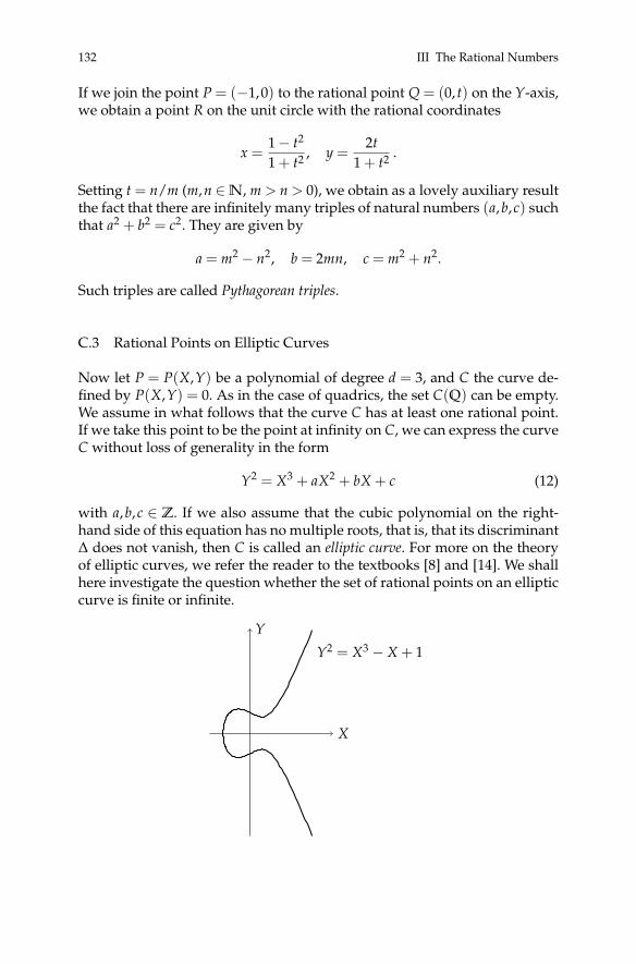
132 III The Rational Numbers
If we join the point P = (−1,0) to the rational point Q = (0, t) on the Y-axis,we obtain a point R on the unit circle with the rational coordinates
x =1− t2
1 + t2 , y =2t
1 + t2 .
Setting t = n/m (m,n ∈N, m > n > 0), we obtain as a lovely auxiliary resultthe fact that there are infinitely many triples of natural numbers (a,b, c) suchthat a2 + b2 = c2. They are given by
a = m2 − n2, b = 2mn, c = m2 + n2.
Such triples are called Pythagorean triples.
C.3 Rational Points on Elliptic Curves
Now let P = P(X,Y) be a polynomial of degree d = 3, and C the curve de-fined by P(X,Y) = 0. As in the case of quadrics, the set C(Q) can be empty.We assume in what follows that the curve C has at least one rational point.If we take this point to be the point at infinity on C, we can express the curveC without loss of generality in the form
Y2 = X3 + aX2 + bX + c (12)
with a,b, c ∈ Z. If we also assume that the cubic polynomial on the right-hand side of this equation has no multiple roots, that is, that its discriminant∆ does not vanish, then C is called an elliptic curve. For more on the theoryof elliptic curves, we refer the reader to the textbooks [8] and [14]. We shallhere investigate the question whether the set of rational points on an ellipticcurve is finite or infinite.
X
Y
Y2 = X3 − X + 1
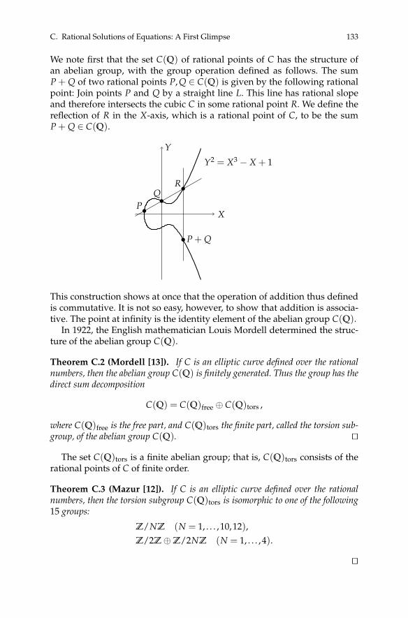
C. Rational Solutions of Equations: A First Glimpse 133
We note first that the set C(Q) of rational points of C has the structure ofan abelian group, with the group operation defined as follows. The sumP + Q of two rational points P, Q ∈ C(Q) is given by the following rationalpoint: Join points P and Q by a straight line L. This line has rational slopeand therefore intersects the cubic C in some rational point R. We define thereflection of R in the X-axis, which is a rational point of C, to be the sumP + Q ∈ C(Q).
X
Y
Y2 = X3 − X + 1
PQ
R
P + Q
This construction shows at once that the operation of addition thus definedis commutative. It is not so easy, however, to show that addition is associa-tive. The point at infinity is the identity element of the abelian group C(Q).
In 1922, the English mathematician Louis Mordell determined the struc-ture of the abelian group C(Q).
Theorem C.2 (Mordell [13]). If C is an elliptic curve defined over the rationalnumbers, then the abelian group C(Q) is finitely generated. Thus the group has thedirect sum decomposition
C(Q) = C(Q)free ⊕ C(Q)tors ,
where C(Q)free is the free part, and C(Q)tors the finite part, called the torsion sub-group, of the abelian group C(Q). ut
The set C(Q)tors is a finite abelian group; that is, C(Q)tors consists of therational points of C of finite order.
Theorem C.3 (Mazur [12]). If C is an elliptic curve defined over the rationalnumbers, then the torsion subgroup C(Q)tors is isomorphic to one of the following15 groups:
Z/NZ (N = 1, . . . ,10,12),Z/2Z⊕Z/2NZ (N = 1, . . . ,4).
ut
134 III The Rational Numbers
For the free part, one has the isomorphism
C(Q)free∼= ZrC = Z⊕ · · · ⊕Z︸ ︷︷ ︸
rC times
.
The number rC is called the rank of C(Q). If rC = 0, then C(Q) has onlyfinitely many rational points. If, on the other hand, we have rC > 0, thenC(Q) has rational points of infinite order and therefore infinitely many ra-tional points. In sum, we have
rC = 0 ⇐⇒ #C(Q) < ∞,rC > 0 ⇐⇒ #C(Q) = ∞.
The problem of describing the group C(Q) of elliptic curves C consists,therefore, essentially in determining its rank rC.
C.4 The Conjecture of Birch and Swinnerton-Dyer
As before, let C be an elliptic curve defined by an equation of the form (12).The conjecture of Birch and Swinnerton-Dyer provides an analytic tool todecide whether rC = 0 or rC > 0. To formulate the conjecture, we now con-sider (12) as a congruence modulo an arbitrary prime number p ∈ P anddefine the quantity
Np := #{
x,y ∈ {0, . . . , p− 1} | y2 ≡ x3 + ax2 + bx + c mod p}+ 1.
In [2], Bryan Birch and Peter Swinnerton-Dyer gave experimental evidencefor the equivalence
rC > 0 ⇐⇒ ∏p∈Pp≤x
Np
p−−−→x→∞
∞. (13)
Using the L-series LC(s) of the elliptic curve C, which for s ∈C with Re(s)>3/2 is defined by the convergent Euler product
LC(s) := ∏p∈P
p -2∆
11− (p + 1− Np)p−s + p1−2s ,
one can rewrite (13), at least formally, as the equivalence
rC > 0 ⇐⇒ LC(1) = 0.
C. Rational Solutions of Equations: A First Glimpse 135
After these preliminaries, we are in a position to formulate the conjecture ofBirch and Swinnerton-Dyer.
Conjecture (Birch–Swinnerton-Dyer conjecture [2]). Let C be an ellipticcurve defined by (12). Then we have the following:(i) The L-series LC(s) of C can be analytically continued to an entire function of
the complex plane C. In particular LC(s) is defined at the point s = 1.(ii) For the order ords=1LC(s) of vanishing of LC(s) at the point s = 1, one has
the equality rC = ords=1LC(s). Moreover, there is an explicit formula thatrelates the first nonvanishing coefficient of the Taylor development of LC(s) ats = 1 to the arithmetic of the curve C.
Aside from a few special cases, this conjecture has been proved essen-tially only for elliptic curves of ranks 0 and 1. More precisely, the followingresults are known. In 1977, John Coates and Andrew Wiles proved in [4] thefiniteness of C(Q) for elliptic curves C/Q with complex multiplication andLC(1) 6= 0. In 1986, Benedict Gross and Don Zagier proved in [7] that (mod-ular) elliptic curves C/Q with LC(1) = 0 but L′C(1) 6= 0 have infinitely manyrational points. Using this result and some new ideas, Victor AlexandrovichKolyvagin proved in 1989, in [9], that LC(1) 6= 0 implies rC = 0, and thatLC(1) = 0, L′C(1) 6= 0 implies rC = 1. His proof required an analytic assump-tion that was shortly afterward proved by Daniel Bump, Solomon Friedberg,and Jeffrey Hoffstein in [3]. We refer the reader to the survey article [17] byAndrew Wiles.
The most current results on the Birch–Swinnerton-Dyer conjecture canbe found in the fundamental works of Manjul Bhargava, for which he wasawarded the Fields Medal in 2014, the highest honor that can be bestowedon a mathematician. Together with Christopher Skinner and Wei Zhang, heproved in [1] that more than 66% of elliptic curves defined over Q satisfy theBirch–Swinnerton-Dyer conjecture.
The search for rational points on elliptic curves is related to the classicalcongruent number problem, which can be formulated simply as follows: LetF be a positive natural number. Is there a right triangle with rational sidelengths a,b, c and area F? That is, do there exist positive rational numbersa,b, c that satisfy the equations
a2 + b2 = c2,a · b
2= F ?
The Pythagorean triple (3,4,5) shows, for example, that for F = 6, there ex-ists such a triangle, in fact, one with not merely rational, but integral, sidelengths. If there exists such a rational right triangle for a given positive nat-ural number F, then we call F a congruent number. The congruent numberproblem is to determine whether a given number F is a congruent number.
The congruent number problem is related to the search for rational pointson elliptic curves as follows. We associate the positive natural number F

136 III The Rational Numbers
with the elliptic curve
CF : Y2 = X3 − F2X = X(X− F)(X + F).
It can be shown that F is a congruent number if and only if the rank rCF of CFis positive, which by the Birch–Swinnerton-Dyer conjecture is equivalent tothe vanishing of LCF (1). If rCF > 0, then there exists a rational point (x,y) ∈CF(Q) with y 6= 0 (since (x,0) would be a 2-torsion point on CF). We note,however, that conversely, if (x,y)∈ CF(Q) is a rational point with y 6= 0, then(x,y) has infinite order, since all rational points of finite order on CF canbe shown to be 2-torsion points and hence satisfy y = 0. We may thereforeassume without loss of generality that x < 0 and y > 0, and we obtain theside lengths of the desired right triangle with area F in the form
a =F2 − x2
y, b = −2xF
y, c =
F2 + x2
y.
Example C.4. For F = 5, the rational point (−5/9,100/27) ∈ CF(Q) has infi-nite order. We therefore obtain the right triangle with side lengths a = 20/3,b = 3/2, c = 41/6 and area F = 5.
For F = 6, we obtain for (−3,9) ∈ CF(Q) the familiar right triangle withsides of length a = 3, b = 4, c = 5.
For F = 1,2,3, it can be shown that rCF = 0, and so 1,2,3 are not congruentnumbers. Since F = 1 is not a congruent number, it follows that there is noright triangle with rational side lengths and area equal to the square of aninteger.
Some known results: If F satisfies one of the congruences F≡ 5,6,7 mod 8,then, as shown in [7], F is a congruent number if L′CF
(1) 6= 0. This conditionis satisfied, for instance, if F is a prime number with F ≡ 5,7 mod 8 (in thelatter case, 2F is also a congruent number). The most current result as thisbook goes to press is that of Ye Tian, who showed in [16] that for everypositive natural number k, there exist infinitely many square-free congruentnumbers F with exactly k distinct prime factors in each of the residue classesF ≡ 5,6,7 mod 8.
If, on the other hand, we have F ≡ 1,2,3 mod 8, it is conjectured that F isnot a congruent number. This conjecture has been proved in the case that Fis prime with F ≡ 3 mod 8 and in a number of additional cases, thanks tothe latest work of Ye Tian, Xinyi Yuan, and Shouwu Zhang.
C.5 Rational Points on Curves of Degree d > 3: Fermat’s Conjecture
We devote the last section of our tour d’horizon to answering our question (B)for algebraic curves C defined by a polynomial P ∈Z[X,Y] of degree d > 3.

C. Rational Solutions of Equations: A First Glimpse 137
To simplify the presentation, we assume that the curve C is nonsingular, thatis, that there exist no points (x,y) ∈ C such that
∂P∂X
(x,y) = 0 and∂P∂Y
(x,y) = 0
hold simultaneously. If we furthermore add the points at infinity to C andassume that the curve is nonsingular at those points as well, we obtain asmooth plane projective curve of degree d > 3, which we again denote byC. Louis Mordell conjectured in his work [13] mentioned above that in thiscase, C(Q) is finite. In 1983, a good sixty years later, Gerd Faltings publisheda proof of this conjecture that earned him a Fields Medal.
Theorem C.5 (Faltings’s theorem [6]). For a smooth plane projective curve Cof degree d > 3 defined over the rational numbers, the set of rational points is finite.
ut
Remark C.6. Faltings’s theorem applies not only to plane algebraic curves.To formulate the theorem in its general form, we recall that associated withevery smooth projective curve C is a natural number gC called the genus ofthe curve. In the case of a smooth plane projective curve C of degree d, thegenus gC is given by the formula
gC =(d− 1)(d− 2)
2.
The general form of Faltings’s theorem states that for a smooth projectivecurve C of genus gC > 1 defined over the rational numbersQ or over any al-gebraic number field K, the set ofQ-rational, respectively K-rational, pointsis finite.
Example C.7. A well-known example is the curve Cd defined by
P(X,Y) = Xd + Yd − 1
with d > 3. Faltings’s theorem states that each curve Cd has only finitelymany rational points.
Fermat’s famous conjecture from the seventeenth century tightens Falt-ings’s finiteness result for this example, since it states that
Cd(Q) =
{{(1,0), (0,1)}, for d odd,{(±1,0), (0,±1)}, for d even.
A complete proof of Fermat’s conjecture, however, was given only in 1995,by Andrew Wiles.
138 III The Rational Numbers
Theorem C.8 (Wiles’s theorem [18]). For d > 2, the equation
Xd + Yd = Zd
has no integer solutions x,y,z with xyz 6= 0. ut
For an overview of Wiles’s proof of Fermat’s last theorem and significantcontributions by other mathematicians, see the articles [10] and [11]. A moreadvanced treatment can be found in [5].
This completes our brief look at answers to question (B) in the search forrational solutions to polynomial equations in two variables, which has pro-vided a glimpse at the very rich arithmetic results that such a search yields.We also have seen that many questions on this topic remain unanswered.
The search for answers to questions (A) and (B) in the general case ofarbitrary systems of polynomials in several variables is a topic of currentresearch. In this case as well, one hopes that the answers will provide inter-esting arithmetic insights.
References
[1] M. Bhargava, C. Skinner, W. Zhang: A majority of elliptic curves over Q satisfy theBirch and Swinnerton-Dyer conjecture. Preprint, July 17, 2014. Available online atarXiv:1407.1826.
[2] B. Birch, H. P. F. Swinnerton-Dyer: Notes on elliptic curves I, II. J. Reine Angew.Math. 212 (1963), 7–25; 218 (1965), 79–108.
[3] D. Bump, S. Friedberg, J. Hoffstein: Non-vanishing theorems for L-functions ofmodular forms and their derivatives. Invent. Math. 102 (1990), 543–618.
[4] J. Coates, A. Wiles: On the conjecture of Birch and Swinnerton-Dyer. Invent. Math.39 (1977), 223–251.
[5] G. Cornell, J. H. Silverman, G. Stevens (eds.): Modular forms and Fermat’s lasttheorem. Springer, Berlin Heidelberg New York, 1997.
[6] G. Faltings: Endlichkeitssätze für abelsche Varietäten. Invent. Math. 73 (1983), 349–366.
[7] B. Gross, D. Zagier: Heegner points and derivatives of L-series. Invent. Math. 84(1986), 225–320.
[8] A.W. Knapp: Elliptic curves. Math. Notes 40, Princeton University Press, Prince-ton, New Jersey, 1992.
[9] V. A. Kolyvagin: On the Mordell–Weil and Shafarevich–Tate groups for elliptic Weilcurves. Math. USSR, Izv. 33 (1989), 473–499.
[10] J. Kramer: Über den Beweis der Fermat-Vermutung I, II. Elem. Math. 50 (1995),12–25; 53 (1998), 45–60.
[11] J. Kramer: Fermat’s last theorem – the solution of a 300 year old problem. In:M. Aigner, E. Behrends (eds.), Mathematics Everywhere, 175–183. AmericanMathematical Society, Providence, Rhode Island, 2010.
[12] B. Mazur: Modular curves and the Eisenstein ideal. Publ. Math. IHES 47 (1977),33–186.

C. Rational Solutions of Equations: A First Glimpse 139
[13] L. J. Mordell: On the rational solutions of the indeterminate equations of the third andfourth degrees. Proc. Cambridge Philos. Soc. 21 (1922), 179–192.
[14] J. H. Silverman, J. Tate: Rational points on elliptic curves. Springer, Cham, 2ndedition, 2015.
[15] I. Stewart, D. Tall: Algebraic number theory and Fermat’s last theorem. Chapmanand Hall/CRC, 4th edition, 2015.
[16] Y. Tian: Congruent numbers and Heegner points. Cambridge J. Math. 2 (2014),117–161.
[17] A. Wiles: The Birch and Swinnerton-Dyer conjecture. Available online atwww.claymath.org/sites/default/files/birchswin.pdf.
[18] A. Wiles: Modular elliptic curves and Fermat’s last theorem. Ann. Math. 141 (1995),443–551.
IV The Real Numbers
1. Decimal Representation of Rational Numbers
Let a be a nonzero natural number. At the end of Chapter I, we used repeateddivision with remainder to represent a in the form
a =`
∑j=0
qj · 10j, (1)
with natural numbers 0 ≤ qj ≤ 9 (j = 0, . . . , `) and q` 6= 0. For the sum (1),we introduced the decimal representation
a = q`q`−1 . . . q1q0.
This decimal notation can be carried over easily to the integers. Namely, ifthe integer a is negative, then a = −|a|. Thus the decimal representation ofthe natural number |a| gives us the decimal representation of a in the form
a = −q`q`−1 . . . q1q0,
again with natural numbers 0≤ qj ≤ 9 (j = 0, . . . , `) and q` 6= 0.We wish now to extend decimal representation to the rational numbers.
To this end, let ab represent a rational number; that is, a, b ∈ Z and b 6= 0.
Without loss of generality, we may assume that b > 0. Using division withremainder for integers, we find for a, b integers q, r with 0≤ r < b such that
a = q · b + r ⇐⇒ ab= q +
rb
.
For the integers q, we have the decimal representation
q = ±`
∑j=0
qj · 10j = ±q`q`−1 . . . q1q0.
We now consider the decimal representation of the rational number 0≤ rb <
1. We assume even that 0 < rb < 1. We rewrite this as
rb=
110· 10 · r
b(2)
© Springer International Publishing AG 2017
Springer Undergraduate Mathematics Series, https://doi.org/10.1007/978-3-319-69429-0_4J. Kramer and A.-M. von Pippich, From Natural Numbers to Quaternions,

142 IV The Real Numbers
and divide 10 · r with remainder by b. We thereby obtain natural numbersq−1, r−1 with 0≤ r−1 < b such that
10 · r = q−1 · b + r−1 ⇐⇒ 10 · rb
= q−1 +r−1
b. (3)
From the inequality rb < 1, we estimate
0≤ q−1 =10 · r
b− r−1
b<
10 · rb
< 10,
that is, 0≤ q−1 ≤ 9. Substituting (3) into (2) leads to
rb=
110· 10 · r
b=
110
(q−1 +
r−1
b
)=
q−1
10+
110· r−1
b=
q−1
10+
1102 ·
10 · r−1
b.
If r−1 6= 0, we divide 10 · r−1 with remainder by b and obtain natural num-bers q−2, r−2 with 0≤ r−2 < b such that
10 · r−1 = q−2 · b + r−2 ⇐⇒ 10 · r−1
b= q−2 +
r−2
b.
As before, we estimate 0≤ q−2 ≤ 9 and putting everything together, obtain
rb=
q−1
10+
1102 ·
10 · r−1
b=
q−1
10+
1102
(q−2 +
r−2
b
)=
q−1
10+
q−2
102 +1
103 ·10 · r−2
b.
Proceeding, we obtain natural numbers q−3,r−3 with 0 ≤ q−3 ≤ 9 and 0 ≤r−3 < b such that
rb=
q−1
10+
q−2
102 +q−3
103 +1
104 ·10 · r−3
b.
After k steps, we obtain natural numbers q−k,r−k with 0 ≤ q−k ≤ 9 and 0 ≤r−k < b such that
rb=
k
∑j=1
q−j
10j +1
10k+1 ·10 · r−k
b.
With this procedure there are two possibilities: either there exists k ∈N, k >0, such that r−k = 0, or the remainders r−j are nonzero for all j = 1, 2, 3, . . . .
Definition 1.1. With notation as above, we define the following for a, b ∈ Zand b 6= 0:(i) If r = 0 or there exists k ∈N, k > 0, with r−k = 0, we set

1. Decimal Representation of Rational Numbers 143
±q` . . . q0.q−1 . . . q−k := ±k
∑j=−`
q−j
10j
and call ±q` . . . q0.q−1 . . . q−k the decimal representation or decimal expan-sion of the rational number a
b .(ii) If all the r−j are nonzero, we set, formally,
±q` . . . q0.q−1 . . . q−k . . . := ±∞
∑j=−`
q−j
10j
and call ±q` . . . q0.q−1 . . . q−k . . . the decimal representation or decimal ex-pansion of the rational number a
b .
Remark 1.2. We note that the infinite sum (series) in Definition 1.1 (ii),
±∞
∑j=−`
q−j
10j = ±(
q` · 10` + · · ·+ q0 +q−1
10+
q−2
102 + · · ·)
,
makes no sense at the present moment. It is merely a symbolic notation. Incontrast, the finite sum in Definition 1.1 (i),
±k
∑j=−`
q−j
10j = ±(
q` · 10` + · · ·+ q0 +q−1
10+ · · ·+ q−k
10k
),
has a concrete significance and takes on the value ab ; that is, we have by
construction that ab= ±q` . . . q0.q−1 . . . q−k.
Definition 1.3. We call a nonterminating decimal expansion
±q` . . . q0.q−1 . . . q−k . . .
periodic if there exist natural numbers v ≥ 0 and p > 0 such that q−(v+j) =q−(v+j+p) = q−(v+j+2p) = · · · for j = 1, . . . , p. For brevity, we write this asfollows:
±q` . . . q0.q−1 . . . q−v q−(v+1) . . . q−(v+p) .
If v = 0, the decimal expansion is said to be purely periodic. The smallest nat-ural number p as defined above is called the period of the decimal expansionof the rational number a
b .
Proposition 1.4. Let a, b ∈ Z, b 6= 0. If the decimal expansion of ab does not ter-
minate, then it is periodic.
Proof. Suppose the number ab has a nonterminating decimal expansion. Look-
ing at the construction of the decimal expansion of ab , we see that the infi-

144 IV The Real Numbers
nite collection of remainders r0 := r, r−1, r−2, r−3, . . . is actually a subset of{0, . . . , b− 1}. Therefore, there must be at least two remainders r−j1 , r−j2 thatare identical. We may assume without loss of generality that j2 > j1 ≥ 0 andfor fixed j1, choose the difference p := j2 − j1 to be minimal. The algorithmfor obtaining the decimal expansion of a
b then shows that
r−j1 = r−(j1+p) = r−(j1+2p) = · · · ,r−(j1+1) = r−(j1+1+p) = r−(j1+1+2p) = · · · ,
· · ·r−(j1+p−1) = r−(j1+2p−1) = r−(j1+3p−1) = · · · .
If we now choose j1 to be minimal and set v := j1 ≥ 0, we obtain the assertionof the theorem. ut
Remark 1.5. The following questions arise:(i) Is there a set of numbers in which the formal infinite sum
±∞
∑j=−`
q−j
10j
can be given a precise meaning?(ii) Is there a set of numbers in which arbitrary infinite decimal expan-
sions, that is, those that are not necessarily periodic, have a well-definedmeaning, that is, in which infinite sums like
±∞
∑j=−`
q−j
10j
represent well-defined numbers?
Exercise 1.6.(a) Determine the decimal expansions of 1
5 , 13 , 1
16 , 111 , and 1
7 .(b) Formulate a criterion for when a fraction a
b (a, b ∈ Z; b 6= 0) possesses aterminating decimal expansion.
(c) Find a bound on the maximal period length of the decimal expansion ofa rational number as a function of its denominator. Give examples forwhich the period is maximal (with respect to this bound).
(d) Describe a process for obtaining the fraction ab from its periodic decimal
expansion. Use this process on the periodic decimal fraction 0.123.

2. Construction of the Real Numbers 145
2. Construction of the Real Numbers
In Chapter I, we constructed the set N of natural numbers on the basis ofthe Peano axioms, and we defined on that set the operations of addition andmultiplication, which satisfy the commutative, associative, and distributivelaws. In particular, we obtained (N, +) as a regular abelian semigroup,which we then, in Chapter II, extended to the abelian group (Z, +) of in-tegers. By carrying over the multiplicative structure of the natural numbersto the integers, we obtained, at the beginning of Chapter III, the integral do-main (Z,+, ·) of integers. We extended this at the end of Chapter III to thefield (Q,+, ·) of rational numbers. In the previous section, we have seen thatthe decimal expansion of a rational number either terminates or is periodic,and that led us to wonder whether there exists a set of numbers containingnumbers with infinite aperiodic decimal expansions. We shall now answerthat question in the affirmative. In doing so, we will be led to the construc-tion of the real numbers. We begin with the definition of a Cauchy sequence.
But first let us specify a few notational conventions. In what follows,we shall use Latin letters to denote rational numbers, which will be dis-tinguished from the real numbers, which we have yet to introduce, whichwill be denoted by Greek letters. The one exception will be the Greek letterepsilon, which in the set of rational numbers will be denoted by ε, and inthe set of real numbers, by ε.
Definition 2.1. A sequence (an) = (an)n≥0 with an ∈Q for all n∈N is calleda rational Cauchy sequence if for every ε ∈Q, ε > 0, there exists N(ε) ∈N suchthat for all m, n ∈Nwith m, n > N(ε), we have the inequality
|am − an| < ε.
A sequence (an) = (an)n≥0 with an ∈ Q for all n ∈ N is called a rationalnull sequence if for every ε ∈Q, ε > 0, there exists N(ε) ∈N such that for alln ∈Nwith n > N(ε), we have the inequality
|an| < ε.
Exercise 2.2.(a) Prove that the sequences
(1
n+1
)n≥0
and( n
2n
)n≥0 are rational null se-
quences.(b) Give further examples of rational null sequences.
Remark 2.3. (i) A rational null sequence (an) is, in particular, a rationalCauchy sequence. Namely, given ε/2 ∈ Q, ε > 0, there exists N(ε/2) ∈ Nsuch that for all m, n ∈Nwith m, n > N(ε/2), we have the inequality
|an| <ε
2.

146 IV The Real Numbers
Using the triangle inequality, we thereby obtain for m, n > N(ε/2) that
|am − an| ≤ |am|+ |an| <ε
2+
ε
2= ε.
Thus (an) is a rational Cauchy sequence.(ii) Every rational Cauchy sequence (an) is bounded, since for ε = 1 and
the associated N(1) ∈ N, which exists by the definition of a Cauchy se-quence, we have for all m, n ∈Nwith m, n > N(1), the inequality
|am − an| < 1.
From this, we obtain with m1 = N(1) + 1 and n > N(1) the bound
|an| = |an − am1 + am1 | ≤ |am1 − an|+ |am1 | < 1 + |am1 |.
We have, therefore, for all n ∈N, the inequality
|an| ≤max{|a0|, . . . , |aN(1)|, 1 + |am1 |}.
This proves the boundedness of the rational Cauchy sequence (an).
We consider now the set M of all rational Cauchy sequences, that is,
M ={(an)
∣∣ (an) is a rational Cauchy sequence}
.
We define on the set M operations of addition and multiplication, which wedenote by + and ·, as follows. For two rational Cauchy sequences (an), (bn),we set
(an) + (bn) := (an + bn) and (an) · (bn) := (an · bn).
We must, of course, convince ourselves that the sum and product of tworational Cauchy sequences are again rational Cauchy sequences. This willbe proved in the following lemma.
Lemma 2.4. Let (an), (bn) ∈ M. Then we have
(an) + (bn) ∈ M and (an) · (bn) ∈ M.
Proof. (i) We first prove that the sum (an) + (bn) of the two rational Cauchysequences (an), (bn) is again a rational Cauchy sequence. To this end, weobserve that the sums an + bn are rational for all n ∈N. We now choose anarbitrary ε ∈ Q, ε > 0, and note that there exist natural numbers N1(ε/2)and N2(ε/2) such that for all m, n > N := max{N1(ε/2), N2(ε/2)}, we havethe inequalities
|am − an| <ε
2and |bm − bn| <
ε
2.

2. Construction of the Real Numbers 147
It now follows from the bound
|(am + bm)− (an + bn)| ≤ |am − an|+ |bm − bn| <ε
2+
ε
2= ε,
for m, n > N, that (an + bn) is a rational Cauchy sequence, and so, therefore,is the sum (an) + (bn).
(ii) We prove now that the product (an) · (bn) of the two rational Cauchysequences (an), (bn) is also a rational Cauchy sequence. We note first that theproducts an · bn are rational for all n ∈ N. Remark 2.3, on the boundednessof rational Cauchy sequences, allows us to find c ∈Q such that for all n ∈N,we have the inequalities
|an| ≤ c and |bn| ≤ c.
Now choose an arbitrary ε ∈ Q, ε > 0, and observe that there exist nat-ural numbers N1
(ε/(2c)
)and N2
(ε/(2c)
)such that for all m, n > N :=
max{N1(ε/(2c)
), N2
(ε/(2c)
)}, we have the inequalities
|am − an| <ε
2cand |bm − bn| <
ε
2c.
We thereby obtain, for all m, n > N, the bound
|am · bm − an · bn| = |am · bm − am · bn + am · bn − an · bn|= |am · (bm − bn) + bn · (am − an)|≤ |am · (bm − bn)|+ |bn · (am − an)|= |am| · |bm − bn|+ |bn| · |am − an|≤ c · ε
2c+ c · ε
2c= ε.
Therefore, (an · bn) is a rational Cauchy sequence, which proves that theproduct (an) · (bn) is a rational Cauchy sequence. ut
Lemma 2.5. The set of rational Cauchy sequences M together with the additiveand multiplicative operations + and ·, that is, (M,+, ·), is a commutative ringwith unit element.
Proof. (i) We show first that (M, +) is an abelian group. We observe first thatM is not empty, since it contains the rational Cauchy sequence (0), consist-ing solely of zeros. The associativity of addition follows at once from theassociativity of addition of rational numbers. Namely, if we have (an), (bn),(cn) ∈ M, then we have also
148 IV The Real Numbers((an) + (bn)
)+ (cn) = (an + bn) + (cn) =
((an + bn) + cn
)=(an + (bn + cn)
)= (an) + (bn + cn)
= (an) +((bn) + (cn)
).
The commutativity of addition also follows at once from that of additionof rational numbers. The rational Cauchy sequence (0) mentioned above,consisting solely of zeros, is clearly the additive identity element, since for(an) ∈ M, we have
(0) + (an) = (0 + an) = (an) = (an + 0) = (an) + (0).
If (an) ∈ M, then we assert that the rational Cauchy sequence (−an) is theadditive inverse of (an). Indeed, we have
(−an) + (an) = (−an + an) = (0) = (an − an) = (an) + (−an).
We have thus shown that (M, +) is an abelian group.(ii) We now show that (M, ·) is an abelian monoid. We begin by noting
that M is nonempty, since it contains the rational Cauchy sequence (1), con-sisting solely of ones. The associativity of multiplication of sequences fol-lows at once from the associativity of multiplication of rational numbers.Namely, if (an), (bn), (cn) ∈ M, then we have(
(an) · (bn))· (cn) = (an · bn) · (cn) =
((an · bn) · cn
)=(an · (bn · cn)
)=(an) · (bn · cn
)= (an) ·
((bn) · (cn)
).
The commutativity of multiplication of sequences follows easily from that ofmultiplication of rational numbers. The rational Cauchy sequence (1) men-tioned above, consisting solely of ones, is clearly the multiplicative identityelement in (M, ·), since for (an) ∈ M, we have
(1) · (an) = (1 · an) = (an) = (an · 1) = (an) · (1).
We have thus proved that (M, ·) is an abelian monoid.(iii) The validity of the distributive laws for M follows easily from the
distributive laws for the rational numbers. For example, for (an), (bn), (cn)∈M, we have
(an) ·((bn) + (cn)
)= (an) · (bn + cn) =
(an · (bn + cn)
)= (an · bn + an · cn) = (an) · (bn) + (an) · (cn).
The proof of the lemma is thus complete. ut
Remark 2.6. If we associate with a rational number r the rational Cauchysequence (r), the sequence consisting solely of r’s, we obtain a mapping

2. Construction of the Real Numbers 149
f :Q−→ M. One may easily check that f is a ring homomorphism
f : (Q,+, ·) −→ (M,+, ·).
Since clearly, ker( f ) = {0}, the ring homomorphism f is injective.
Definition 2.7. We set
n :={(an) ∈ M
∣∣ (an) is a rational null sequence}
and call this set the ideal of rational null sequences. This name is justified bythe following lemma.
Lemma 2.8. The ideal n of rational null sequences is an ideal in the commutativering (M,+, ·).
Proof. (i) We must first convince ourselves that (n, +) is a subgroup of(M, +). Since the rational Cauchy sequence (0), consisting solely of zeros,is a rational null sequence, it follows that n is not empty. Invoking the sub-group criterion, Lemma 2.25 of Chapter II, we see that it suffices to showthat for (an), (bn) ∈ n, the difference (an)− (bn) is also in n. Since (an) and(bn) are rational null sequences, there exist for ε ∈ Q, ε > 0, natural num-bers Na(ε/2) and Nb(ε/2) such that for all n > Na(ε/2) and n > Nb(ε/2),we have the inequalities
|an| <ε
2and |bn| <
ε
2.
It follows then from the triangle inequality that we have
|an − bn| <ε
2+
ε
2= ε
for n > max{Na(ε/2), Nb(ε/2)}. That is, (an) − (bn) is a rational null se-quence. Therefore, (n, +) is a subgroup of (M, +).
(ii) Our second task is to show that the product of a rational null se-quence (bn) ∈ n and a rational Cauchy sequence (an) ∈M is again a rationalnull sequence. Since the rational Cauchy sequence (an) is bounded, by Re-mark 2.3 (ii), there exists c ∈ Q, c > 0, such that for all n ∈ N, we have theinequality |an| ≤ c. For an arbitrary ε∈Q, ε > 0, there then exists N(ε/c)∈Nsuch that for all n > N(ε/c), we have the inequality
|an · bn| = |an| · |bn| ≤ c · ε
c= ε.
Therefore, (an) · (bn) is in fact a rational null sequence, and that completesthe proof that n is an ideal of (M,+, ·). ut

150 IV The Real Numbers
Remark 2.9. We may now apply Theorem 3.21 of Chapter III to the commu-tative ring (M,+, ·) of rational Cauchy sequences and the ideal n of rationalnull sequences and obtain the commutative quotient ring (M/n,+, ·). Theelements of M/n are cosets of the form
α = (an) + n,
where (an) is a rational Cauchy sequence. The elements of each coset arerational Cauchy sequences, and the difference of each pair of elements inthe coset is a rational null sequence.
Definition 2.10. Let (an) be a rational sequence, and 0 ≤ n0 < n1 < n2 <· · ·< nk < · · · an increasing sequence of natural numbers. The sequence (ank )is called a subsequence of the sequence (an).
Lemma 2.11. Let (an) be a rational Cauchy sequence, and (ank ) a subsequence of(an). Then we have
(ak)− (ank ) = (ak − ank ) ∈ n.
Proof. Let ε ∈Q, ε > 0. Since (an) is a rational Cauchy sequence and nk ≥ k,there exists a natural number N(ε) such that for all k > N(ε), we have theinequality
|ak − ank | < ε.
This shows that the sequence (ak − ank ) is a rational null sequence, whichcompletes the proof. ut
Theorem 2.12. The quotient ring (M/n,+, ·) is a field.
Proof. By construction, the zero and unit elements of M/n are given by
(0) + n and (1) + n,
where (0) and (1) denote the rational Cauchy sequences that consist solelyof zeros and ones respectively.
Since we have already established that (M/n,+, ·) is a commutative ringwith unit element (1) + n, it remains only to show that every coset (an) + nother than the zero element of M/n, that is, for which we have
(an) + n 6= (0) + n ⇐⇒ (an) /∈ n,
has a multiplicative inverse. Since (an) /∈ n, there exist ε0 ∈ Q, ε0 > 0, andN(ε0) ∈N such that for all n > N(ε0), we have the inequality
|an| > ε0, or equivalently, an 6= 0. (4)
We therefore define the rational sequence (bn) by

2. Construction of the Real Numbers 151
bn :=
0, 0≤ n ≤ N(ε0),1an
, n > N(ε0).
We show first that (bn) is a rational Cauchy sequence and then that one canconstruct a multiplicative inverse to (an) + n.
For m, n > N(ε0), we obtain, using (4),
|bm − bn| =∣∣∣∣ 1am− 1
an
∣∣∣∣ = |am − an||am · an|
<|am − an|
ε20
.
Since (an) is a rational Cauchy sequence, there exists for ε ∈ Q, ε > 0, anumber N(ε2
0 · ε) such that for all m, n > N(ε20 · ε), we have
|am − an| < ε20 · ε.
We thereby obtain at once, for all m, n > max{N(ε0), N(ε20 · ε)} the inequal-
ity|bm − bn| < ε;
that is, we indeed have (bn) ∈ M.Finally, we claim that the element (bn) + n is the multiplicative inverse of
(an) + n. To prove this, we have only to show that((an) + n
)·((bn) + n
)= (1) + n,
that is, that (an) · (bn)− (1) ∈ n. For n > N(ε0), we have by construction that
an · bn = 1;
that is, the rational Cauchy sequence (an) · (bn)− (1) consists solely of zerosafter the first N(ε0) terms, and it is therefore a rational null sequence. ut
Definition 2.13. We call the field (M/n,+, ·) the field of real numbers anddenote it byR. In what follows, we shall denote the elements ofR by Greekletters. For example, we have
α ∈R ⇐⇒ α = (an) + n,
for some (an) ∈ M.
Lemma 2.14. The mapping that assigns to every rational number r the real num-ber (r) + n, where (r) is the rational Cauchy sequence each term of which is equalto r, induces an injective ring homomorphism
F : (Q,+, ·) −→ (R,+, ·).
Proof. For r1, r2 ∈Q, we verify at once that
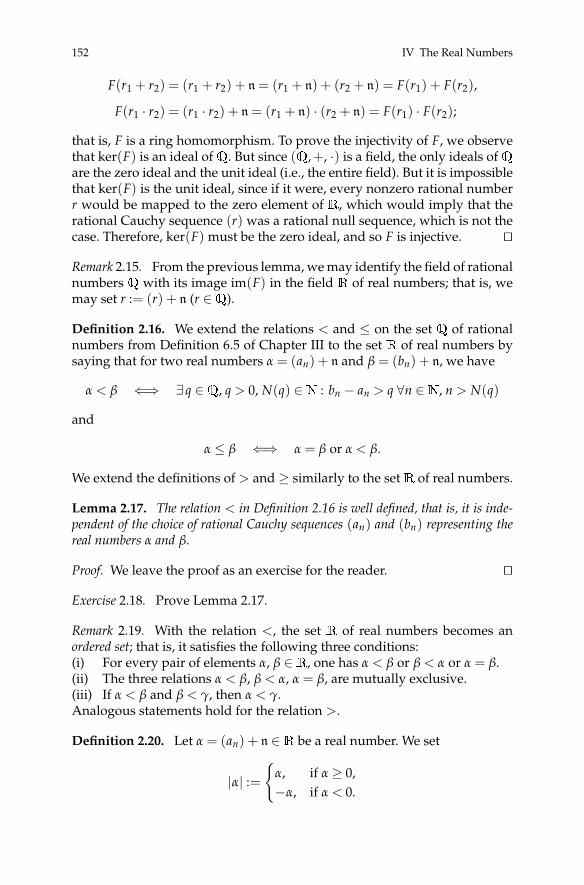
152 IV The Real Numbers
F(r1 + r2) = (r1 + r2) + n= (r1 + n) + (r2 + n) = F(r1) + F(r2),
F(r1 · r2) = (r1 · r2) + n= (r1 + n) · (r2 + n) = F(r1) · F(r2);
that is, F is a ring homomorphism. To prove the injectivity of F, we observethat ker(F) is an ideal ofQ. But since (Q,+, ·) is a field, the only ideals ofQare the zero ideal and the unit ideal (i.e., the entire field). But it is impossiblethat ker(F) is the unit ideal, since if it were, every nonzero rational numberr would be mapped to the zero element of R, which would imply that therational Cauchy sequence (r) was a rational null sequence, which is not thecase. Therefore, ker(F) must be the zero ideal, and so F is injective. ut
Remark 2.15. From the previous lemma, we may identify the field of rationalnumbers Q with its image im(F) in the field R of real numbers; that is, wemay set r := (r) + n (r ∈Q).
Definition 2.16. We extend the relations < and ≤ on the set Q of rationalnumbers from Definition 6.5 of Chapter III to the set R of real numbers bysaying that for two real numbers α = (an) + n and β = (bn) + n, we have
α < β ⇐⇒ ∃q ∈Q, q > 0, N(q) ∈N : bn − an > q ∀n ∈N, n > N(q)
and
α ≤ β ⇐⇒ α = β or α < β.
We extend the definitions of > and ≥ similarly to the setR of real numbers.
Lemma 2.17. The relation < in Definition 2.16 is well defined, that is, it is inde-pendent of the choice of rational Cauchy sequences (an) and (bn) representing thereal numbers α and β.
Proof. We leave the proof as an exercise for the reader. ut
Exercise 2.18. Prove Lemma 2.17.
Remark 2.19. With the relation <, the set R of real numbers becomes anordered set; that is, it satisfies the following three conditions:(i) For every pair of elements α, β ∈R, one has α < β or β < α or α = β.(ii) The three relations α < β, β < α, α = β, are mutually exclusive.(iii) If α < β and β < γ, then α < γ.Analogous statements hold for the relation >.
Definition 2.20. Let α = (an) + n ∈R be a real number. We set
|α| :={
α, if α ≥ 0,−α, if α < 0.

2. Construction of the Real Numbers 153
We call the real number |α| the absolute value of the real number α .
Lemma 2.21. The absolute value on the real numbers satisfies the following prop-erties:(i) |α · β| = |α| · |β| for all α, β ∈R.(ii) |α + β| ≤ |α|+ |β| for all α, β ∈R.
Proof. We leave the proof as an exercise for the reader. ut
Exercise 2.22. Prove Lemma 2.21.
We carry over the notion of a rational Cauchy sequence to the field(R,+, ·) of real numbers.
Definition 2.23. A sequence (αn) = (αn)n≥0 such that αn ∈R for all n ∈Nis called a real Cauchy sequence if for every ε ∈R, ε > 0, there exists N(ε) ∈Nsuch that for all m, n ∈Nwith m, n > N(ε), we have the inequality
|αm − αn| < ε.
Remark 2.24. Let (αn) be a real Cauchy sequence. The nth term of the se-quence, αn, is then given by αn = (an,k) + n, where (an,k) is a rational Cauchysequence. Moreover, ε ∈ R, ε > 0, is of the form ε = (εk) + n with the ratio-nal Cauchy sequence (εk). Using Definition 2.16 with the relation <, Def-inition 2.23 now takes the form that for m, n ∈ N with m, n > N(ε), thereexists a natural number M(m, n) such that for all k > M(m, n), we have theinequality
|am,k − an,k| < εk.
Exercise 2.25. Give examples of real null sequences whose terms are all ir-rational (that is, not rational) numbers.
Definition 2.26. A real sequence (αn) has a limit α ∈R , or equivalently, thesequence converges to α ∈ R, if for every ε ∈ R, ε > 0, there exists a naturalnumber N(ε) such that for all n ∈Nwith n > N(ε), we have the inequality
|αn − α| < ε.
In this case, we writeα = lim
n→∞αn.
Theorem 2.27. In the field (R,+, ·) of real numbers, every real Cauchy sequence(αn) has a limit α ∈R.
Proof. By Remark 2.24, we have αn = (an,k) + n with the rational Cauchysequence (an,k). We shall show that
154 IV The Real Numbers
(i) the rational sequence (an,n) is a Cauchy sequence;(ii) we have limn→∞ αn = α, where α := (an,n) + n.
(i) Let ε ∈ R, ε > 0; without loss of generality, we may choose ε to berational; that is, we may have ε = (ε) with ε∈Q. By Remark 2.24, there existsfor all m, n > N(ε), a natural number M(m, n) such that for all k > M(m, n),we have the inequality
|am,k − an,k| < ε.
We now show that there exists a natural number N0(ε) such that the in-equality
|am,k − an,k| < ε
holds for all m, n > N0(ε) and all k ∈ N. To this end, we observe first of allthat the rational Cauchy sequence (an,k) representing αn can be altered bypassage to a subsequence, which for simplicity we again denote by (an,k), insuch a way that
|an,k − an,n| <1n
(5)
for all k∈N. It then follows by the triangle inequality that for arbitrary k, k′ ∈N, we have
|an,k − an,k′ | ≤ |an,k − an,n|+ |an,n − an,k′ | <2n
.
We thereby obtain for all m, n > N(ε/2), k ∈N, and k′ > M(m, n) the bound
|am,k − an,k| ≤ |am,k − am,k′ |+ |am,k′ − an,k′ |+ |an,k′ − an,k|
<2m
+ε
2+
2n
.
If we now set N0(ε) := max{
N( ε2 ), [
8ε ]}
, we obtain, as desired, for all m, n >N0(ε) and all k ∈N, the bound
|am,k − an,k| < ε. (6)
If we now choose m, n > N0(ε) and set k = m in the inequalities (6) and (5),we obtain
|am,m − an,n| ≤ |am,m − an,m|+ |an,m − an,n|
< ε +1n< ε +
ε
8< 2ε.
We have thus shown that (an,n) is a rational Cauchy sequence by which wedefine the real number α; that is, we have α := (an,n) + n.
(ii) It remains to show that limn→∞ αn = α. Again let ε∈Q, ε > 0. We mustshow that for sufficiently large n,k, we have the inequality

3. The Decimal Expansion of a Real Number 155
|an,k − ak,k| < ε. (7)
Setting m = k into (6) and then choosing n, k > N0(ε), we obtain the desiredinequality (7), that is,
|αn − α| < ε
for all n > N0(ε). This proves the assertion. ut
Definition 2.28. Because of the fact proved in the previous theorem thatevery real Cauchy sequence in the field (R,+, ·) has a limit that itself is inR, we say that the real numbers are complete.
Remark 2.29. Let α = (an) + n ∈ R be a real number. The rational Cauchysequence (an) is in particular also a real Cauchy sequence, which we mayalso denote by (an) because we have identified Q with a subset of the realnumbersR. The proof of Theorem 2.27 shows that
α = limn→∞
an;
that is, every real number is the limit of a rational Cauchy sequence.
Exercise 2.30. Find a rational Cauchy sequence with limit√
2.
3. The Decimal Expansion of a Real Number
Definition 3.1. Let q−j be natural numbers with 0≤ q−j ≤ 9 for
j = −`, . . . , 0, 1, 2, . . .
and ` ∈N. Then we call the formal sum
±q` . . . q0.q−1q−2 . . . := ±∞
∑j=−`
q−j · 10−j
an (infinite) decimal. We set
D′ := {±q` . . . q0.q−1q−2 . . . | ±q` . . . q0.q−1q−2 . . . is a decimal}.
The decimal ±q` . . . q0.q−1q−2 . . . is said to be terminating if there exists anindex k≥ 0 such that q−j = 0 for j > k. The notion of periodicity of a decimalexpansion and the associated notions from Definition 1.3 can be carried overto decimals without further ado.
Remark 3.2. On the basis of our previous considerations, terminating andperiodic decimals can be identified with rational numbers. The remain-ing decimals have no clear meaning at this point. However, the following

156 IV The Real Numbers
lemma will allow us to identify them with real numbers. To this end, wemake an association between the set D′ of decimals and the set R of realnumbers.
Lemma 3.3. Let±q` . . . q0.q−1q−2 . . . be a decimal and (an) the rational sequencegiven by
an := ±q` . . . q0.q−1 . . . q−n.
With the assignment
±q` . . . q0.q−1q−2 . . . 7→ (an) + n,
we obtain a surjective mapping of sets
ϕ : D′ −→R.
Proof. (i) We must first demonstrate that the mapping ϕ is well defined, thatis, that the sequence (an) is a rational Cauchy sequence. To this end, let ε ∈Q, ε > 0, and N ∈N be such that 10−N < ε. Then by construction, we havethat for all m, n > N with m > n,
|am − an| < 0.0 . . . 0q−(n+1) . . . q−m < 10−N < ε,
which proves the Cauchy sequence property.(ii) We now prove the surjectivity of ϕ. It suffices to show that ϕ yields a
surjective mapping of the set of all nonnegative decimals
q` . . . q0.q−1q−2 . . . ∈D′
to the set of nonnegative real numbers. To construct a decimal expansion ofa given real number, we shall try to imitate the procedure given in Section 1for obtaining the decimal expansion of a rational number. However, we donot have, in general, division with remainder at our disposal. As a substi-tute, we shall use the fact that we can decompose a real number into itsinteger part and fractional part, the latter being nonnegative and less than 1.
Suppose, then, that we have α ∈R with α≥ 0. There then exist q ∈N andρ ∈R with 0≤ ρ < 1 such that
α = q + ρ.
For the natural number q, we have the decimal representation
q =`
∑j=0
qj · 10j = q`q`−1 . . . q1q0.
We writeρ =
110· 10 · ρ
3. The Decimal Expansion of a Real Number 157
and decompose 10 · ρ as before in the form
10 · ρ = q−1 + ρ−1
with q−1 ∈N and ρ−1 ∈ R with 0≤ ρ−1 < 1; since we have ρ < 1, it followsthat 0≤ q−1 ≤ 9. We thereby obtain
ρ =1
10(q−1 + ρ−1
)=
q−1
10+
ρ−1
10.
We again write10 · ρ−1 = q−2 + ρ−2,
where q−2 ∈N with 0≤ q−2 ≤ 9 and ρ−2 ∈R with 0≤ ρ−2 < 1. This yields
ρ =q−1
10+
1102
(q−2 + ρ−2
)=
q−1
10+
q−2
102 +ρ−2
102 .
Proceeding in this way, we obtain the decimal expansion
q` . . . q0.q−1q−2 . . . ∈D′.
The partial sumsan = q` . . . q0.q−1 . . . q−n
of this decimal expansion form a rational Cauchy sequence, which by con-struction, converges in R to α. We thereby see that
ϕ(q` . . . q0.q−1q−2 . . . ) = α.
This proves the surjectivity of ϕ. ut
Remark 3.4. The proof of the preceding Lemma 3.3 shows that the decimal±q` . . . q0.q−1q−2 . . . corresponds to the real number
α = ± limn→∞
n
∑j=−`
q−j · 10−j = ±∞
∑j=−`
q−j · 10−j
via the mapping ϕ. We have thus answered in the affirmative the questionraised in Section 1 of this chapter about the possible meaning of such series.
Remark 3.5. We now investigate the mapping ϕ : D′ −→R from Lemma 3.3with respect to injectivity. We shall see that ϕ is not injective. It will thereforebe our goal to measure the defect in injectivity. In what follows, we mayagain restrict our attention to the set of nonnegative decimals.
Lemma 3.6. Let
q` . . . q0.q−1q−2 . . . and q′`′ . . . q′0.q′−1q′−2 . . .

158 IV The Real Numbers
be nonnegative decimals such that
ϕ(q` . . . q0.q−1q−2 . . . ) = ϕ(q′`′ . . . q′0.q′−1q′−2 . . . ), (8)
where ϕ is the set mapping from D′ to R defined in Lemma 3.3. Then either the twodecimals are identical, or one of the two terminates and the other consists solely of9’s from some point in its decimal expansion onward.
Proof. We may, without loss of generality, assume `′ ≥ `. By Remark 3.4, weobtain from (8) the equality
q′`′ · 10`′+ · · ·+ q′`+1 · 10`+1 =
∞
∑j=−`
(q−j − q′−j) · 10−j.
If we divide this equation by 10`+1, we shall see that without loss of gener-ality, we may assume that ` = −1. We thus obtain
q′`′ · 10`′+ · · ·+ q′0 =
∞
∑j=1
(q−j − q′−j) · 10−j. (9)
Since 0≤ qj, q′j ≤ 9, we may estimate the right-hand side of (9), obtaining
0≤∣∣∣∣ ∞
∑j=1
(q−j − q′−j) · 10−j∣∣∣∣ ≤ ∞
∑j=1|q−j − q′−j| · 10−j ≤ 9 ·
∞
∑j=1
10−j
= 9( ∞
∑j=0
10−j − 1)= 9(
11− 1
10− 1)= 9(
109− 1)= 1.
We therefore obtain
0≤(q′`′ · 10`
′+ · · ·+ q′0
)≤ 1
for the left-hand side of (9); that is, we have `′ = 0 and q′0 = 1 or `′ = −1,whence q′0 = 0. Since the first case obtains precisely when equality holds inthe previous inequality for all j = 1, 2, . . . , we see that this case obtains onlyif for j = 1, 2, . . . , we have the equality
|q−j − q′−j| = 9.
Since this is all taking place with nonnegative numbers, this means that
q−j = 9 and q′−j = 0 (j = 1, 2, . . . ).
If the latter case obtains, then we proceed from the equality q0 = q′0 and lookfor an index −k such that q−k = q′−k, yet q−k−1 6= q′−k−1. Either there is nosuch index, in which case the two decimals are identical, or there indeed

4. Equivalent Characterizations of Completeness 159
exists such an index −k; if we then argue as above, we see that the decimal0, q−1q−2 . . . consists solely of 9’s from the (k + 1)st decimal place onward.
ut
Definition 3.7. We now define D⊂D′ as the subset containing no decimalscontaining only 9’s from some point on. We shall call the elements of D
genuine decimals.
Theorem 3.8. There is a bijection between the set D of genuine decimals and thesetR of real numbers.
Proof. The theorem follows directly from Lemmas 3.3 and 3.6. ut
Remark 3.9. Using Theorem 3.8, we may henceforward speak of the decimalrepresentation or decimal expansion of real numbers.
Moreover, with the help of the bijection between D and R from Theo-rem 3.8, we may carry over addition and multiplication of real numbers tothe set of genuine decimals. We thereby obtain the field (D,+, ·) of genuinedecimals.
Remark 3.10. Using the decimal representation of real numbers, it can beshown that the setR is uncountable. We are not going to discuss this further,and we refer the reader to the relevant literature. Since the set Q of rationalnumbers is countable, the set difference R \Q is not empty. This fact leadsto the following definition.
Definition 3.11. A real number α ∈R \Q is said to be irrational.
Exercise 3.12.(a) Think about why the number 0.101001000100001 . . . (that is, the num-
ber of zeros between ones is successively 1,2,3, . . . ) is irrational. Givefurther examples of irrational decimals.
(b) Compute the first ten decimal places of√
2 precisely.
4. Equivalent Characterizations of Completeness
In this section, we shall present some equivalent characterizations of thecompleteness of the real numbers. This will lead us to the notions of supre-mum and infimum.
Definition 4.1. A real sequence (αn) is said to be monotonically increasing iffor all n ∈ N, we have the inequality αn+1 ≥ αn, and it is said to be strictlymonotonically increasing if we have αn+1 > αn.

160 IV The Real Numbers
A real sequence (αn) is said to be monotonically decreasing if for all n ∈N,we have the inequality αn+1 ≤ αn, and it is said to be strictly monotonicallydecreasing if we have αn+1 < αn.
Exercise 4.2. Determine which of the following sequences are (strictly) mo-notonically increasing or (strictly) monotonically decreasing:(
121
n+1
)n≥0
,(
n3 − 2n2 − 2
)n≥0
,(
n2 + 22n
)n≥0
,(
n3 + 33n
)n≥0
,(
n1
n+1
)n≥0
.
Definition 4.3. A nonempty set M ⊆ R is said to be bounded from above ifthere exists γ ∈R such that for all µ ∈M, we have µ ≤ γ. The real numberγ is called an upper bound for the set M.
A nonempty set M ⊆ R is said to be bounded from below if there existsγ ∈R such that for all µ ∈M, we have µ ≥ γ. The real number γ is called alower bound for the set M.
A nonempty set M ⊆ R is said to be bounded if it is bounded both fromabove and from below.
Theorem 4.4. If a nonempty set M ⊆ R is bounded from above, then the set Mhas a least upper bound σ ∈R.
Proof. We choose α0 ∈R such that α0 is not an upper bound for M but suchthat β0 := α0 + 1 is such an upper bound. Then α0 +
12 is either an upper
bound for M or it is not. In the first case, we define
α1 := α0 and β1 := α0 +12
,
while in the second case, we define
α1 := α0 +12
and β1 := β0.
Proceeding in this fashion, we construct inductively two real sequences (αn)and (βn) that satisfy the following three properties:(1) The sequence (αn) is monotonically increasing.(2) The sequence (βn) is monotonically decreasing.(3) For all m, n ∈N, we have the inequality αn ≤ βm.
Choose now ε ∈R, ε > 0, and m ∈N such that 2−m < ε. Then for all n ∈Nwith n > m, we have by the nature of our construction that
|αm − αn| = αn − αm ≤ βm − αm ≤1
2m < ε.
We see, then, that (αn) is a real Cauchy sequence. Analogously, we see that(βn) is also a real Cauchy sequence. We set

4. Equivalent Characterizations of Completeness 161
α := limn→∞
αn, β := limn→∞
βn.
Sincelim
n→∞(βn − αn) = 0,
we conclude that α = β.We now claim that α is the desired least upper bound for the set M. Since
the real numbers βn are by construction upper bounds for M for all n ∈N,we have for all µ ∈M and n ∈N the inequality
µ ≤ βn,
that is,µ ≤ β = α.
Thus α is an upper bound for M.Now let ε ∈ R, ε > 0, be such that α′ := α − ε is a smaller upper bound
for M. By the monotonicity of the sequence (αn), we can find N(ε) ∈N suchthat for all n > N(ε), we have the inequality
αn ≥ α− ε = α′ .
But since αn by construction cannot be an upper bound for M for all n ∈N,there must exist µn ∈M such that µn > αn. If we now choose n > N(ε), weobtain the contradiction µn > α′. Therefore, α is the least upper bound forM, and the theorem is proved. ut
One can prove analogously the following theorem.
Theorem 4.5. If a nonempty set M ⊆ R is bounded from below, then the set Mhas a greatest lower bound σ ∈R. ut
Exercise 4.6. Give an example showing that there is no valid analogue ofTheorem 4.5 for the set of rational numbers.
Exercise 4.7. Find the greatest lower bound and the least upper bound forthe set { x
√x | x ∈Q, x ≥ 0}.
Definition 4.8. The least upper bound for a nonempty set M that is boundedabove, as described above in Theorem 4.4, is called the supremum of M andis denoted by sup(M).
The greatest lower bound for a nonempty set M that is bounded below iscalled the infimum of M and is denoted by inf(M).
Definition 4.9. A sequence of closed intervals
[αn, βn] := {δ ∈R | αn ≤ δ ≤ βn} ⊆R (n ∈N)

162 IV The Real Numbers
is called a sequence of nested intervals if the real sequences (αn) and (βn)satisfy the following three properties:(1) The sequence (αn) is monotonically increasing.(2) The sequence (βn) is monotonically decreasing.(3) We have the limit limn→∞(βn − αn) = 0.
Theorem 4.10. If the intervals [αn, βn] ⊆R for n ∈N form a sequence of nestedintervals, then we have
∞⋂n=0
[αn, βn] = {α}
for some real number α.
Proof. We begin by showing that the intersection
∞⋂n=0
[αn, βn]
is nonempty. To this end, we consider the nonempty set
A := {αn | n ∈N} ⊆R and B := {βn | n ∈N} ⊆R.
By definition, the set A is bounded from above, namely by the elements ofB. Similarly, the set B is bounded from below. By Theorems 4.4 and 4.5, wemay consider the supremum of A and the infimum of B, that is,
α := sup(A) ∈R and β := inf(B) ∈R.
By property (3) in Definition 4.9, we must have α = β. Since αn ≤ α = β≤ βnfor all n ∈N, we have found with α an element that belongs to every interval[αn, βn] (n ∈N).
We now show that α is the only element in the intersection under discus-sion. To this end, let γ ∈ ⋂∞
n=0[αn, βn] be arbitrary. Since αn ≤ γ ≤ βn for alln ∈N, we have
α = limn→∞
αn ≤ γ ≤ limn→∞
βn = β,
which shows that α = γ. ut
Remark 4.11. We may paraphrase the result of Theorem 4.10 by saying thatthe nested intervals principle holds in R. We have seen that the completenessof the real numbers, called the completeness principle, has as a consequencethe existence of a supremum (supremum principle) and an infimum (infimumprinciple), which in turn implies the nested intervals principle. We close thiscircle by showing that the nested intervals principle implies completeness.In sum, in the set of real numbers, the following are equivalent:– the completeness principle,

4. Equivalent Characterizations of Completeness 163
– the supremum and infimum principles,– the nested intervals principle.
Theorem 4.12. Consider the set (R,+, ·) of real numbers with its order relation< and assume the validity of the nested intervals principle. Then every real Cauchysequence (αn) has a limit in R; that is, the nested intervals principle implies thecompleteness principle.
Proof. Let ε ∈ R, ε > 0. Then there exists N(ε) ∈ N such that for all naturalnumbers m, n > N(ε), we have the inequality
|αm − αn| < ε.
If n0 := N(ε) + 1, then for all natural numbers n ≥ n0, we have
|αn − αn0 | < ε,
that is,|αn| < |αn0 |+ ε.
Settingµ := max{|α0|, . . . , |αn0−1|, |αn0 |+ ε},
we see that M := {αn | n ∈N} ⊆R is a bounded set; that is, there exist realnumbers µ0, ν0 such that for all n ∈N, we have the inequalities
µ0 ≤ αn ≤ ν0.
By repeated halving of the closed interval [µ0, ν0], we obtain a sequence ofnested intervals [µk, νk] (k ∈ N) such that infinitely many terms of the se-quence lie in each of the intervals; that is, for infinitely many indices n, wehave
µk ≤ αn ≤ νk.
The assumed validity of the nested intervals principle implies the existenceof a real number α that is determined by
∞⋂k=0
[µk, νk] = {α}.
There exists, therefore, a natural number K(ε) such that for all natural num-bers k > K(ε), we have the inequalities
α− ε < µk < νk < α + ε;
that is, for infinitely many indices m, we have the inequalities
α− ε < αm < α + ε ⇐⇒ |αm − α| < ε.

164 IV The Real Numbers
Increasing N(ε) if necessary, we may choose one of the infinitely many in-dices m = n0 and obtain
|αn0 − α| < ε.
It therefore follows that for all natural numbers n > N(ε), we have
|αn − α| ≤ |αn − αn0 |+ |αn0 − α| < 2ε.
This proves the convergence of the real Cauchy sequence (αn) and that theequality
limn→∞
αn = α
holds. ut
5. The Real Numbers and the Real Number Line
In this section, we shall construct a bijection between the elements of the setof real numbers and the points on a straight line. This will lead us to the no-tion of the real number line. To do so, we shall require the classical axioms ofplane Euclidean geometry. We shall use in particular that the plane consistsof points, that through every two points in the plane there passes exactly onestraight line and this line determines a unique line segment (connecting thetwo points), and that two distinct lines in the plane have exactly one pointof intersection unless they are parallel. We shall also require the fact that wecan mark off segments on a line using a compass. We shall also assume thevalidity of the important similarity theorems. We shall see, however, thatthe classical axioms do not suffice for carrying out our desired identificationof the set of real numbers with a straight line. We shall need an additionalaxiom, which we shall call the axiom of geometric completeness.
We begin with the set R of real numbers and a horizontal straight line Gin the plane. Our goal is to produce a bijection from the setR of real numbersto the line G. We begin by choosing a point P0 on the line G, which we callthe zero point. We choose the point P0 ∈ G as the image of the zero element0 ∈R.
G�
P0
After marking off an arbitrary but fixed unit distance on the line, we canmark equidistant points on the line G, beginning from the zero point P0 andmoving to the right, a unit distance apart, which we consider the images ofthe natural numbers 1, 2, 3, . . . . We denote these points by P1, P2, P3, . . . . Byreflecting in the zero point P0, we obtain the images of the negative integers−1,−2,−3, . . . on G, which we denote by P−1, P−2, P−3, . . . .
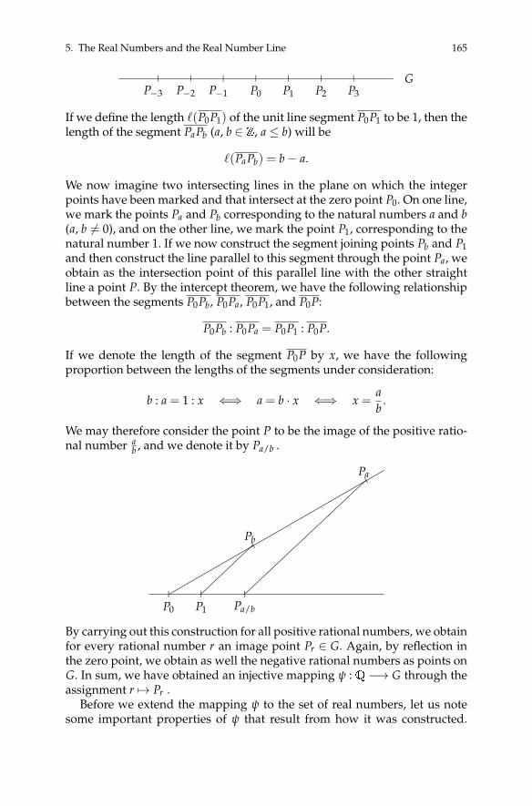
5. The Real Numbers and the Real Number Line 165
G�
P0
�
P3
�
P2
�
P1
�
P−1
�
P−2
�
P−3
If we define the length `(P0P1) of the unit line segment P0P1 to be 1, then thelength of the segment PaPb (a, b ∈ Z, a ≤ b) will be
`(PaPb) = b− a.
We now imagine two intersecting lines in the plane on which the integerpoints have been marked and that intersect at the zero point P0. On one line,we mark the points Pa and Pb corresponding to the natural numbers a and b(a, b 6= 0), and on the other line, we mark the point P1, corresponding to thenatural number 1. If we now construct the segment joining points Pb and P1and then construct the line parallel to this segment through the point Pa, weobtain as the intersection point of this parallel line with the other straightline a point P. By the intercept theorem, we have the following relationshipbetween the segments P0Pb, P0Pa, P0P1, and P0P:
P0Pb : P0Pa = P0P1 : P0P.
If we denote the length of the segment P0P by x, we have the followingproportion between the lengths of the segments under consideration:
b : a = 1 : x ⇐⇒ a = b · x ⇐⇒ x =ab
.
We may therefore consider the point P to be the image of the positive ratio-nal number a
b , and we denote it by Pa/b .
�
P0
�
P1
1Pb
�
Pa/b
1Pa
By carrying out this construction for all positive rational numbers, we obtainfor every rational number r an image point Pr ∈ G. Again, by reflection inthe zero point, we obtain as well the negative rational numbers as points onG. In sum, we have obtained an injective mapping ψ :Q−→ G through theassignment r 7→ Pr .
Before we extend the mapping ψ to the set of real numbers, let us notesome important properties of ψ that result from how it was constructed.

166 IV The Real Numbers
First, ψ preserves the order relation < on Q in the sense that for rationalnumbers r, s with r < s, the image point Pr lies to the left of the image pointPs. Moreover, the mapping ψ respects the addition and multiplication ofrational numbers. For example, for two positive rational numbers r, s, weobtain the image point Pr+s of the sum r + s as the point of G obtained as theconcatenation of the segments P0Pr and P0Ps. The difference of two rationalnumbers is interpreted similarly. The point Pr·s corresponding to the productr · s of two (positive) rational numbers r, s can be constructed by a suitableapplication of the intercept theorem to the segments P0Pr, P0Ps.
We are ready now to extend the mapping ψ : Q −→ G to the set R ofreal numbers. For simplicity of notation, we shall continue to denote thisextended mapping by ψ. We begin by defining the image of an interval[r, s] ⊆ R with rational endpoints r, s as the set of points on the segmentPrPs ⊆ G, that is,
ψ([r, s]) = PrPs.
We note that the length of the segment PrPs is given by
`(PrPs) = s− r.
Now let α∈R be an arbitrary real number. The construction of the real num-bers together with the nested intervals principle shows that we can obtainα as the intersection of the intervals In = [an, bn] (n ∈ N) of a sequence ofnested intervals with rational endpoints. The intervals In = [an, bn] (n ∈ N)are mapped by ψ to the segments Pan Pbn . To continue the mapping ψ fromQ toR, we require at this point an additional axiom.
Definition 5.1. The line G satisfies the axiom of geometric completeness if ev-ery sequence of nested line segments Pan Pbn (n ∈N) with
limn→∞
`(
Pan Pbn
)= 0
has a nonempty intersection, that is, if we have
∞⋂n=0
Pan Pbn 6= ∅. (10)
Remark 5.2. We see that the intersection (10) in Definition 5.1 consists of asingle point P∈G: First of all, the intersection (10) is nonempty by the axiomof geometric completeness. For the sake of obtaining a contradiction, let ussuppose that the intersection (10) contains at least the two points P, Q. Thesetwo points are separated by some positive distance d > 0. If we choose nlarge enough, then the length of the segment Pan Pbn will be less than d. Thisleads to a contradiction, since under these conditions, the points P, Q cannotboth belong to the intersection (10).
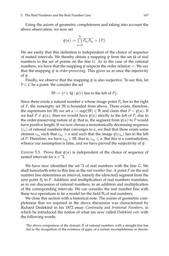
5. The Real Numbers and the Real Number Line 167
Using the axiom of geometric completeness and taking into account theabove observation, we now set
ψ(α) :=∞⋂
n=0Pan Pbn = {P}.
We see easily that this definition is independent of the choice of sequenceof nested intervals. We thereby obtain a mapping ψ from the set R of realnumbers to the set of points on the line G. As in the case of the rationalnumbers, we have that the mapping ψ respects the order relation <. We saythat the mapping ψ is order-preserving. This gives us at once the injectivityof ψ.
Finally, we observe that the mapping ψ is also surjective. To see this, letP ∈ G be a point. We consider the set
M := {r ∈Q | ψ(r) lies to the left of P}.
Since there exists a natural number a whose image point Pa lies to the rightof P, the nonempty set M is bounded from above. There exists, therefore,the supremum for M; we set α := sup(M) ∈ R and claim that P = ψ(α). Ifwe had P 6= ψ(α), then we would have ψ(α) strictly to the left of P, due tothe order-preserving nature of ψ; that is, the segment from ψ(α) to P wouldhave positive length. If we now choose a monotonically decreasing sequence(cn) of rational numbers that converges to α, we find that there exists someelement cn0 such that cn0 > α and such that the image ψ(cn0) lies to the leftof P. Therefore, we have cn0 ∈M, that is, cn0 ≤ α. But this is a contradiction,whence our assumption is false, and we have proved the surjectivity of ψ.
Exercise 5.3. Prove that ψ(α) is independent of the choice of sequence ofnested intervals for α ∈R.
We have now identified the set R of real numbers with the line G. Weshall henceforth refer to this line as the real number line. A point P on the realnumber line determines an interval, namely the (directed) segment from thezero point P0 to P. Addition and multiplication of real numbers translates,as in our discussion of rational numbers, to an addition and multiplicationof the corresponding intervals. We can consider the real number line withthese two operations to be a model for the fieldR of real numbers.
We close this section with a historical note. The axiom of geometric com-pleteness that we required in the above discussion was characterized byRichard Dedekind in his 1872 essay Continuity and Irrational Numbers, inwhich he introduced the notion of what are now called Dedekind cuts withthe following words:
The above comparison of the domain R of rational numbers with a straight line hasled to the recognition of the existence of gaps, of a certain incompleteness or discon-

168 IV The Real Numbers
tinuity of the former, while we ascribe to the straight line completeness, absence ofgaps, or continuity. In what then does this continuity consist? Everything must de-pend on the answer to this question, and only through it shall we obtain a scientificbasis for the investigation of all continuous domains. By vague remarks upon the un-broken connection in the smallest parts obviously nothing is gained; the problem is toindicate a precise characteristic of continuity that can serve as the basis for valid de-ductions. For a long time I pondered over this in vain, but finally I found what I wasseeking. This discovery will, perhaps, be differently estimated by different people; themajority may find its substance very commonplace. It consists of the following. In thepreceding section attention was called to the fact that every point p of the straightline produces a separation of the same into two portions such that every point of oneportion lies to the left of every point of the other.1
6. The Axiomatic Point of View
Definition 6.1. A field (K,+, ·) is said to be ordered if for all α ∈ K, thereexists a relation α > 0 satisfying the following two properties:(i) Exactly one of the following three possibilities holds: α > 0, α = 0, α < 0
(that is, −α > 0).(ii) If we have α, β ∈ K with α, β > 0, then we have α + β > 0 and α · β > 0.
Remark 6.2. If (K,+, ·) is an ordered field, then the order relation allows usto define an absolute value for the elements of K, which in turn allows us tointroduce the notion of a Cauchy sequence (αn) ⊆ K.
Definition 6.3. An ordered field (K,+, ·) is said to be complete if everyCauchy sequence (αn) ⊆ K converges to an element of K.
Remark 6.4. The field R of real numbers is a complete ordered field. As inthe case of the real numbers, completeness in an arbitrary ordered field canalso be characterized in terms of the supremum and infimum principles orthe nested intervals principle.
To complete the chapter, we sketch a proof of a theorem, which goes backto David Hilbert, stating that the field of real numbers R is (up to isomor-phism) the unique complete ordered field.
Theorem 6.5. A complete ordered field (K,+, ·) is uniquely determined up toorder-preserving ring isomorphism; that is, if (K′,+, ·) is an arbitrary completeordered field, then there exists a ring isomorphism
ϕ : (K,+, ·) −→ (K′,+, ·)
1 Translation by Wooster Woodruff Beman, 1901.
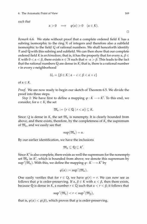
6. The Axiomatic Point of View 169
such thatα > 0 =⇒ ϕ(α) > 0 (α ∈ K).
ut
Remark 6.6. We state without proof that a complete ordered field K has asubring isomorphic to the ring Z of integers and therefore also a subfieldisomorphic to the field Q of rational numbers. We shall henceforth identifyZ andQwith this subring and subfield. We can then show that our completeordered field K is archimedean; that is, it has the property that for every α, β ∈K with 0 < α < β, there exists n ∈N such that n · α > β. This leads to the factthat the rational numbersQ are dense in K; that is, there is a rational numberr in every ε-neighborhood
Uε = {β ∈ K | α− ε < β < α + ε}
of α ∈ K.
Proof. We are now ready to begin our sketch of Theorem 6.5. We divide theproof into three steps.
Step 1: We have first to define a mapping ϕ : K −→ K′. To this end, weconsider, for α ∈ K, the set
Mα := {r ∈Q | r < α} ⊆ K.
Since Q is dense in K, the set Mα is nonempty. It is clearly bounded fromabove, and there exists, therefore, by the completeness of K, the supremumof Mα, and we easily see that
sup(Mα) = α.
By our earlier identification, we have the inclusions
Mα ⊆Q⊆ K′.
Since K′ is also complete, there exists as well the supremum for the nonemptyset Mα in K′, which is bounded from above; we denote this supremum bysup ′(Mα). With this, we define the mapping ϕ : K −→ K′ by
ϕ(α) := sup ′(Mα).
One easily verifies that for r ∈ Q, we have ϕ(r) = r. We can now see asfollows that ϕ is order-preserving. If α, β ∈ K with α < β, then there exists,becauseQ is dense in K, a number r ∈Q such that α < r < β; it follows that
sup ′(Mα) < r < sup ′(Mβ),
that is, ϕ(α) < ϕ(β), which proves that ϕ is order-preserving.

170 IV The Real Numbers
Step 2: We show here that the mapping ϕ is bijective. We begin with theproof of injectivity. If we have α, β ∈ K with α 6= β, then we may assumewithout loss of generality that α < β. Because ϕ is order-preserving, we havealso ϕ(α) < ϕ(β), that is, ϕ(α) 6= ϕ(β), which proves that ϕ is injective.
To show the surjectivity of ϕ, we choose α′ ∈ K′ and consider the setMα′ ⊆ K′, which we also, of course, view as a subset of K. We set α :=sup(Mα′) ∈ K. From the equality
sup(Mα) = α = sup(Mα′),
we see that the sets Mα and Mα′ are identical, whence
ϕ(α) = sup ′(Mα) = sup ′(Mα′) = α′.
This proves that ϕ is surjective.Step 3: We now show that ϕ is a ring homomorphism. We begin with the
additivity of ϕ. For α, β ∈ K, we consider the set
Nα,β := {r + s | r, s ∈Q, r < α, s < β}
and show that Nα,β =Mα+β. Namely, if t := r+ s∈Nα,β, that is, t = r+ s withr, s ∈Q and r < α, s < β, then we have t ∈Q and t < α + β, that is, t ∈Mα+β.That is, we have the inclusion Nα,β ⊆Mα+β. Conversely, if t ∈Mα+β, that is,t ∈Q and t < α + β, then using the density ofQ in K, we can find r ∈Q thatsatisfies
t− β < r < α.
Setting s := t− r, we obtain rational numbers r, s with r < α and s < β. Sincenow t = r + s with r, s ∈ Q and r < α, s < β, we see that we have t ∈ Nα,β,from which follows the inclusion Mα+β ⊆Nα,β.
It follows from the equality of sets Nα,β =Mα+β that
ϕ(α + β) = sup ′(Mα+β) = sup ′(Nα,β). (11)
It remains to show that sup ′(Nα,β) = ϕ(α)+ ϕ(β). To this end, we assert thatϕ(α) + ϕ(β) is an upper bound for Nα,β. Indeed, if t := r + s ∈Nα,β, that is,t = r + s with r, s ∈Q and r < α, s < β, then we have
t = r + s = ϕ(r) + ϕ(s) < ϕ(α) + ϕ(β),
from which follows the assertion. It remains now to show that ϕ(α) + ϕ(β)is the least upper bound for Nα,β. Let K′ 3 γ < ϕ(α) + ϕ(β) be a smallerupper bound for Nα,β. SinceQ is dense in K′, there exist t, r ∈Q such that
γ < t < ϕ(α) + ϕ(β), t− ϕ(β) < r < ϕ(α).

D. The p-adic Numbers: Another Completion ofQ 171
Setting s := t − r, we have obtained rational numbers r, s with r < α ands < β. Since now t = r + s with r, s ∈Q and r < α, s < β, we see that t ∈Nα,β.But since we have also γ < t, it follows that γ cannot be an upper bound forNα,β. Therefore, we have
ϕ(α) + ϕ(β) = sup ′(Nα,β).
The additivity of ϕ now comes from (11). If α > 0, then we obtain in partic-ular from the fact that ϕ is additive and order-preserving that
ϕ(α) > ϕ(0) = 0.
One proceeds similarly to prove the multiplicativity of ϕ. We shall omit theproof. This completes our sketch of the proof of Theorem 6.5. ut
Exercise 6.7. Fill in the missing details in the above proof sketch.
Remark 6.8. If we proceed from the axiomatic point of view, it is not cleara priori that a complete ordered field K even exists. Our construction of thereal numbers R in Section 2 has given us a model of such a field. An alter-native model is provided by the real number line.
D. The p-adic Numbers: Another Completion of
Following our construction of the real numbers, we end this chapter by in-troducing an alternative completion of the rational numbers that will leadus to the set of p-adic numbers. In what follows, we shall discuss the utilityof the p-adic numbers, which will give us interesting new insights that willagain lead us to some current problems in number theory.
D.1 The p-adic Absolute Value
We begin with the definition of the absolute value on the field Q of rationalnumbers.
Definition D.1. A mapping ‖ · ‖ : Q −→ R is called an absolute value if itsatisfies the following three properties:(i) For all r ∈Q, one has ‖r‖ ≥ 0 and ‖r‖ = 0 ⇐⇒ r = 0.(ii) For all r, s ∈Q, one has the product rule ‖r · s‖ = ‖r‖ · ‖s‖.(iii) For all r, s ∈Q, one has the triangle inequality ‖r + s‖ ≤ ‖r‖+ ‖s‖.
Example D.2. (i) The absolute value | · | of a rational number introducedin Definition 6.8 of Chapter III is clearly an absolute value in the above sense.We call it the archimedean absolute value on Q.
Q

172 IV The Real Numbers
(ii) If we define |r|triv := 1 for r ∈ Q, r 6= 0, and set |0|triv := 0, we obtainanother absolute value | · |triv, which we call the trivial absolute value on Q.
Remark D.3. We can construct yet another absolute value, one for eachprime number p, in the following way: If r = a/b is a nonzero rational num-ber, we can write r in the form
r =a′
b′pn,
where a′,b′ are nonzero integers relatively prime to p, and n is an integer(which by the fundamental theorem of arithmetic is uniquely determined).If we now set vp(r) := n and vp(0) := ∞, we obtain a mapping
vp : Q −→Z ∪ {∞},
which clearly possesses the following two properties:(i) For all r, s ∈Q, one has vp(r · s) = vp(r) + vp(s).(ii) For all r, s ∈Q, one has vp(r + s) ≥min(vp(r),vp(s)).We call the mapping vp the p-adic valuation on Q. With it, we define for r ∈Q
the quantity
|r|p := p−vp(r).
Using the properties of the p-adic valuation vp(·), one can verify at oncethat | · |p defines an absolute value. In particular, the validity of the triangleinequality can be seen as follows:
|r + s|p = p−vp(r+s) ≤ p−min(vp(r),vp(s)) = max(|r|p, |s|p) ≤ |r|p + |s|p,
that is, one has in fact the sharper inequality |r + s|p ≤max(|r|p, |s|p), whichis known as the ultrametric inequality.
Definition D.4. We call the absolute value | · |p constructed in the previousremark for an arbitrary prime p the p-adic absolute value on Q.
Remark D.5. If r is a nonzero rational number, then using the definition ofthe p-adic absolute value, one may easily verify the important formula
|r| · ∏p∈P
|r|p = 1,
known as the product formula.
The larger the power n of the prime number p that divides r ∈ Q, thesmaller the p-adic absolute value |r|p of r, and conversely. This is illustratedin the following examples.

D. The p-adic Numbers: Another Completion ofQ 173
Example D.6. (i) Let
r =96
9801=
25 · 31
34 · 112 .
Then v2(r) = 5, v3(r) =−3, v11(r) =−2, and vp(r) = 0 for all primes p suchthat p 6= 2,3,11. It follows that |r|2 = 1
32 , |r|3 = 27, |r|11 = 121, and |r|p = 1for all primes p such that p 6= 2,3,11.
(ii) Let r1 = 735 = 3 · 5 · 72, r2 = 3 · 5 · 712, and r3 = 3 · 5 · 7−10. Then
|r1|7 =149
, |r2|7 =1
712 =1
13841287201, |r3|7 = 710 = 282475249,
but |r1|p = |r2|p = |r3|p for all primes p such that p 6= 7.
We recall that two absolute values ‖ · ‖ and ‖ · ‖′ are said to be equivalentif there exists a positive real number σ such that ‖ · ‖′ = ‖ · ‖σ. With this inmind, we obtain the following theorem, due to Alexander Ostrowski.
Theorem D.7 (Ostrowski [5]). Every nontrivial absolute value
‖ · ‖ : Q −→R
defined on the field Q of rational numbers is equivalent either to the archimedeanabsolute value | · | or to a p-adic absolute value | · |p. ut
Remark D.8. For two distinct primes p,q, the associated absolute values | · |pand | · |q are inequivalent.
D.2 The p-adic Numbers
In analogy to the notions of a rational Cauchy sequence and rational nullsequence that we introduced in Definition 2.1 in relation to the archimedeanabsolute value, we can now also define rational Cauchy sequences and ra-tional null sequences with respect to the p-adic absolute value.
Definition D.9. A sequence (an) = (an)n≥0 with an ∈ Q for all n ∈ N iscalled a rational Cauchy sequence with respect to the p-adic absolute value if forevery ε ∈ Q, ε > 0, there exists N(ε) ∈ N such that for all m, n ∈ N withm, n > N(ε), the inequality
|am − an|p < ε
holds.A sequence (an) = (an)n≥0 with an ∈ Q for all n ∈ N is called a rational
null sequence with respect to the p-adic absolute value if for every ε ∈Q, ε > 0,

174 IV The Real Numbers
there exists N(ε) ∈N such that for all n ∈Nwith n > N(ε), the inequality
|an|p < ε
holds.
Example D.10. (i) The sequence (an) = (7n)n≥0 is a rational null sequencewith respect to the 7-adic absolute value; to see this, one has only to observethat |7n|7 = 7−n holds for all n ∈N. If, on the other hand, p is a prime dif-ferent from 7, then (7n)n≥0 is not a rational null sequence with respect to thep-adic absolute value, although it is a bounded sequence, since in this case,one has |7n|p = 1 for all n ∈N.
(ii) Let p be an arbitrary prime. Then the sequence (an) = ( 1n )n>0 is not
a rational null sequence with respect to the p-adic absolute value, since forthe subsequence (p−m)m≥0, one has∣∣∣ 1
pm
∣∣∣p= pm.
This shows that the sequence (an) = ( 1n )n>0 is not convergent.
(iii) The sequence (an) = (2−n)n≥0 is a bounded sequence with respect tothe 7-adic absolute value. It is not, however, a Cauchy sequence, since∣∣∣ 1
2n −1
2n+1
∣∣∣7=∣∣∣ 12n+1
∣∣∣7= 1.
These examples provide a first impression of a “calculus” of the p-adicabsolute value, known as p-adic analysis, which appears to contradict muchof our experience with real analysis. We refer the interested reader to theliterature on the subject, in particular, the books [1] and [3].
Remark D.11. In analogy to the construction of the real numbers, let us nowconsider the set Mp of all rational Cauchy sequences with respect to the p-acid absolute value, that is,
Mp ={(an)
∣∣ (an) is a rational Cauchy sequence with respect to the p-adic
absolute value}
.
If we equip Mp with a componentwise additive operation + and a multi-plicative operation ·, then (Mp,+, ·) becomes a commutative ring with unitelement. Analogously, we set
np ={(an) ∈ Mp
∣∣ (an) is a rational null sequence with respect to the p-adic
absolute value}
,

D. The p-adic Numbers: Another Completion ofQ 175
and we see that np is an ideal of Mp. As in the case of the archimedeanabsolute value, one can show that the quotient ring (Mp/np,+, ·) is a field.
Definition D.12. We call the field (Mp/np,+, ·) the field of p-adic numbersand denote it by Qp.
The field of p-adic numbers was discovered at the end of the nineteenthcentury by Kurt Hensel.
Theorem D.13. The mapping that associates with every rational number r the p-adic number (r) + np, where (r) denotes the rational Cauchy sequence with respectto the p-adic absolute value whose every term is equal to r, induces an injective ringhomomorphism
Fp : (Q,+, ·) −→ (Qp,+, ·).
Moreover, the field Qp of p-adic numbers is complete; that is, every Cauchy sequence(αn) ⊂ Qp with respect to the p-adic absolute value converges to a limiting valueα ∈Qp. ut
Remark D.14. In analogy to the decimal fraction representation of a realnumber, it can be shown that a p-adic number α ∈ Qp can be representedby a series
α =∞
∑j=`
qj pj
with ` ∈Z and qj ∈ {0, . . . , p− 1} = Fp. The set{α ∈Qp
∣∣∣∣α =∞
∑j=0
qj pj}
is called the set of p-adic integers and denoted by Zp; it can then be seen that(Zp,+, ·) is a commutative subring of the field of p-adic numbers (Qp,+, ·).From the definition of Zp, it can be seen at once that one has an isomorphism
Zp/pZp ∼= Fp.
D.3 The Local–Global Principle
For a polynomial P(X1, . . . , Xn) ∈ Z[X1, . . . , Xn] in the n variables X1, . . . , Xnwith integer coefficients, we called in Appendix C an n-tuple of rationalnumbers (x1, . . . , xn) such that P(x1, . . . , xn) = 0 a rational zero of the poly-nomial P(X1, . . . , Xn). We had previously not investigated the question of

176 IV The Real Numbers
the existence of rational zeros of polynomials. Rather, we considered thequestion of the existence of finitely or infinitely many zeros of polynomialsunder the assumption that at least one such zero existed. In this section, weshall investigate the question of existence by considering some examples.
Remark D.15. As earlier, let P(X1, . . . , Xn)∈Z[X1, . . . , Xn], and let (x1, . . . , xn)∈ Qn be a rational zero of P(X1, . . . , Xn). From the embedding of Q in the p-adic numbers Qp as well as in the real numbers R, the n-tuple (x1, . . . , xn) canalso be viewed as an element of Qn
p or of Rn. We thereby observe that theexistence of a rational zero of P(X1, . . . , Xn) entails the existence of a p-adiczero for all prime numbers p as well as a real zero. This, of course, raises atonce the converse question: If a polynomial P(X1, . . . , Xn) has for all primesp a p-adic zero as well as a real zero, does the polynomial P(X1, . . . , Xn) thennecessarily possess a rational zero?
To simplify the notation, we shall denote the set of real numbers R by Q∞and the archimedean absolute value | · | by | · |∞.
Definition D.16. A polynomial P(X1, . . . , Xn) ∈ Z[X1, . . . , Xn] satisfies thelocal–global principle if the existence of p-adic zeros for all p ∈ P ∪ {∞} im-plies the existence of a rational zero of the polynomial P(X1, . . . , Xn).
If the polynomial P(X1, . . . , Xn) satisfies the local–global principle, thenin the search for rational zeros, we are led to the search for p-adic zeros ofthe polynomial P(X1, . . . , Xn) for all p ∈P∪ {∞}. We shall now consider thisquestion for p ∈ P. We begin by recalling the following simple lemma.
Lemma D.17. Let P(X1, . . . , Xn) ∈ Z[X1, . . . , Xn] be a polynomial and p ∈ P aprime number. Then the following three statements are equivalent:(i) P(X1, . . . , Xn) has a zero in Qn
p,(ii) P(X1, . . . , Xn) has a primitive zero in Zn
p,(iii) P(X1, . . . , Xn) has a zero in (Z/pmZ)n for all m ∈N>0,where a zero (x1, . . . , xn)∈Zn
p is primitive if not all the xj (j = 1, . . . ,n) are divisibleby p. ut
This lemma reduces the question of p-adic zeros of a polynomial to thesolution of polynomial congruences modulo pm for all m ∈N>0 (we refer inthis regard to Section B.2). The following theorem shows under what condi-tions a zero modulo p already gives rise to a p-adic zero.
Theorem D.18. Let P(X1, . . . , Xn) ∈Z[X1, . . . , Xn] be a polynomial and p ∈ P aprime. Then every simple zero of P(X1, . . . , Xn) modulo p induces a p-adic zero ofP(X1, . . . , Xn). Here a zero (x1, . . . , xn) ∈Zn modulo p is called simple if(
∂P∂Xj
(x1, . . . , xn)
)j=1,...,n
6≡ (0, . . . ,0) mod p.

D. The p-adic Numbers: Another Completion ofQ 177
Proof. We carry out the proof first for the case n = 1 and for simplicity ofnotation write X = X1. Let x(0) ∈Z be a simple zero of the polynomial P(X)modulo p. That is, we have
P(x(0)) ≡ 0 mod p, i.e., P(x(0)) = p a with a ∈Z,
P′(x(0)) 6≡ 0 mod p, i.e., P′(x(0)) = b with b ∈Z, (b, p) = 1.
With an integer y yet to be determined, we set x(1) := x(0) + p y and obtain,with the help of Taylor’s formula,
P(x(1)) = P(
x(0))+ p y P′
(x(0)
)+ p2 c = p(a + y b) + p2 c,
for some c ∈ Z. Since b is relatively prime to p, there exists y ∈ Z such thata + y b ≡ 0 mod p. We thereby obtain
P(x(1)) ≡ 0 mod p2 and x(1) ≡ x(0) mod p.
If we proceed in the same way, that is, define x(2) := x(1)+ p2 z with some z∈Z yet to be determined, we obtain a sequence of integers (x(0), x(1), x(2), . . . )for which we have
P(x(j)) ≡ 0 mod pj+1 and x(j+1) ≡ x(j) mod pj+1 (j = 0,1,2, . . . ).
The sequence (x(0), x(1), x(2), . . . ) is clearly a Cauchy sequence with respectto the p-adic absolute value that converges to a p-adic number, say ξ. Byconstruction, we have P(ξ) = 0; that is, ξ is the desired p-adic zero.
Finally, we reduce the case n > 1 to the case n = 1. We begin with the sim-ple zero (x1, . . . , xn) of P(X1, . . . , Xn) modulo p and define for k ∈ {1, . . . ,n}the polynomial
Q(Xk) := P(x1, . . . , xk−1, Xk, xk+1, . . . , xn) ∈Z[Xk].
We then construct as previously, beginning with xk, a p-adic zero ξk of Q(Xk)(with a suitable choice of k). After interpreting the xj as p-adic numbers ξ j(j = 1, . . . ,n; j 6= k), we obtain, as desired, P(ξ1, . . . ,ξn) = 0. This completesthe proof of the theorem. ut
Remark D.19. The method employed in the previous proof of constructinga p-adic zero ξ of the polynomial P(X) by beginning with a zero x(0) ∈ Z
modulo p yields in the case of the field R of real numbers the well-knownNewton’s method of finding the zeros of a polynomial.

178 IV The Real Numbers
D.4 The Theorem of Hasse–Minkowski
In this section, we shall introduce a special class of polynomials for whichthe local–global principle is valid. To this end, we consider the set
Q :={
Q(X1, . . . , Xn) =n
∑j,k=1
aj,kXjXk
∣∣∣∣ aj,k = ak,j ∈Z, det(aj,k) 6= 0}
of nondegenerate quadratic forms over Z. We can now formulate the main the-orem of this section.
Theorem D.20 (Hasse–Minkowski). A quadratic form Q(X1, . . . , Xn) ∈ Qsatisfies the local–global principle. ut
We shall not prove Theorem D.20 here; we refer the interested reader tothe book [7]. Instead, we shall present some examples to indicate how onecan use the Hasse–Minkowski theorem to find nontrivial rational zeros ofnondegenerate quadratic forms over Z.
Remark D.21. Ernst S. Selmer showed that the Hasse–Minkowski theoremcannot, in general, be generalized to cubic polynomials. To that end, he in-troduced the polynomial
P(X1, X2, X3) = 3X31 + 4X3
2 + 5X33 ,
which has nontrivial p-adic zeros for all p ∈P ∪ {∞} but no nontrivial ratio-nal zeros. In contrast, Roger Heath-Brown showed that every cubic form inat least 14 variables satisfies the local–global principle (see [2]). Accordingto an idea introduced by Yuri I. Manin, the obstruction to the validity of thelocal–global principle for cubic forms is measured by the Brauer group, acertain second cohomology group (see [4]). In general, further obstructionsto the validity of the local–global principle for polynomials can arise. Onespeaks in this regard of the Brauer–Manin Obstruction (see [8]).
Remark D.22. By the Hasse–Minkowski theorem, a quadratic form Q(X1, . . . ,Xn) ∈ Q has a nontrivial rational zero if the underlying form has nontriv-ial p-adic zeros for all p ∈ P ∪ {∞}. This raises the question as to how onemight prove the existence of such zeros. In the real case, that is, if p = ∞, thismeans simply that the given quadratic form must be indefinite. For the casep ∈ P with p 6= 2, we have the following sufficient criterion.
Proposition D.23. A nondegenerate quadratic form
Q(X1, . . . , Xn) =n
∑j,k=1
aj,kXjXk ∈ Q
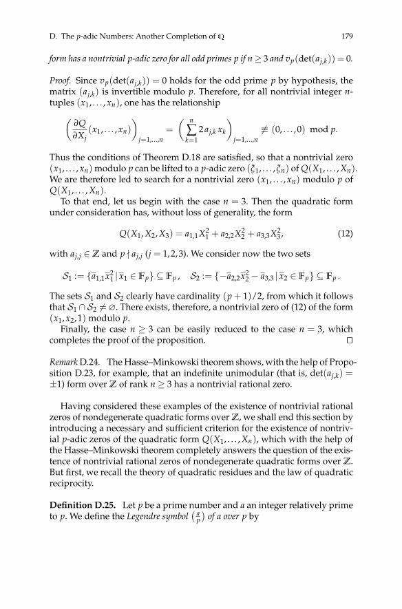
D. The p-adic Numbers: Another Completion ofQ 179
form has a nontrivial p-adic zero for all odd primes p if n≥ 3 and vp(det(aj,k)) = 0.
Proof. Since vp(det(aj,k)) = 0 holds for the odd prime p by hypothesis, thematrix (aj,k) is invertible modulo p. Therefore, for all nontrivial integer n-tuples (x1, . . . , xn), one has the relationship(
∂Q∂Xj
(x1, . . . , xn)
)j=1,...,n
=
( n
∑k=1
2 aj,k xk
)j=1,...,n
6≡ (0, . . . ,0) mod p.
Thus the conditions of Theorem D.18 are satisfied, so that a nontrivial zero(x1, . . . , xn) modulo p can be lifted to a p-adic zero (ξ1, . . . ,ξn) of Q(X1, . . . , Xn).We are therefore led to search for a nontrivial zero (x1, . . . , xn) modulo p ofQ(X1, . . . , Xn).
To that end, let us begin with the case n = 3. Then the quadratic formunder consideration has, without loss of generality, the form
Q(X1, X2, X3) = a1,1X21 + a2,2X2
2 + a3,3X23 , (12)
with aj,j ∈Z and p - aj,j (j = 1,2,3). We consider now the two sets
S1 := {a1,1x21 | x1 ∈ Fp} ⊆ Fp , S2 := {−a2,2x2
2 − a3,3 | x2 ∈ Fp} ⊆ Fp .
The sets S1 and S2 clearly have cardinality (p + 1)/2, from which it followsthat S1 ∩ S2 6=∅. There exists, therefore, a nontrivial zero of (12) of the form(x1, x2,1) modulo p.
Finally, the case n ≥ 3 can be easily reduced to the case n = 3, whichcompletes the proof of the proposition. ut
Remark D.24. The Hasse–Minkowski theorem shows, with the help of Propo-sition D.23, for example, that an indefinite unimodular (that is, det(aj,k) =±1) form over Z of rank n ≥ 3 has a nontrivial rational zero.
Having considered these examples of the existence of nontrivial rationalzeros of nondegenerate quadratic forms over Z, we shall end this section byintroducing a necessary and sufficient criterion for the existence of nontriv-ial p-adic zeros of the quadratic form Q(X1, . . . , Xn), which with the help ofthe Hasse–Minkowski theorem completely answers the question of the exis-tence of nontrivial rational zeros of nondegenerate quadratic forms over Z.But first, we recall the theory of quadratic residues and the law of quadraticreciprocity.
Definition D.25. Let p be a prime number and a an integer relatively primeto p. We define the Legendre symbol
( ap)
of a over p by

180 IV The Real Numbers(ap
):=
{+1, if a is a quadratic residue modulo p,−1, if a is a quadratic nonresidue modulo p.
Here a is a quadratic residue modulo p means that there exists x ∈Z such thatx2 ≡ a mod p; otherwise, a is a quadratic nonresidue modulo p. If p | a, we set( a
p)
:= 0.
Remark D.26. Since the Legendre symbol is multiplicative with respect tothe “numerator,” its evaluation can be reduced to the cases a = −1, a = 2,and a = q (q an odd prime). In the first two cases, one has(−1
p
)=
{+1, if p ≡ +1 mod 4,−1, if p ≡ −1 mod 4,
as well as (2p
)=
{+1, if p ≡ ±1 mod 8,−1, if p ≡ ±3 mod 8.
The calculation of( q
p)
proceeds with the help of the law of quadratic reci-procity: (
qp
)= (−1)
p−12
q−12
(pq
).
The Legendre symbol enables us to calculate the Hilbert symbol, whichwe now define for the field of p-adic numbers Qp.
Definition D.27. For α, β ∈Qp, we consider the quadratic form
−αX21 − βX2
2 + X23 (13)
and define the Hilbert symbol (α, β)p of α, β with respect to Qp as +1 if (13) hasa nontrivial solution (x1, x2, x3) ∈Q3
p and as −1 otherwise.
Remark D.28. The Hilbert symbol (α, β)p can be calculated as follows. Wewrite
α = u · pa, with u ∈Z×p and a ∈Z,
β = v · pb, with v ∈Z×p and b ∈Z;
here we can identify u and v with integers relatively prime to p on accountof the isomorphism Zp/pZp ∼= Z/pZ; we again denote these integers by uand v. Then if p is odd, we have

D. The p-adic Numbers: Another Completion ofQ 181
(α, β)p =
(−1p
)ab(up
)b( vp
)a
.
In the case p = 2, there is an equally simple formula.
Definition D.29. A nondegenerate quadratic form
Q(X1, . . . , Xn) =n
∑j,k=1
aj,kXjXk
defined over Z has two important invariants in addition to its degree n.The first invariant is given by the discriminant disc(Q) of Q, defined by
det(aj,k) mod(Q×)2.The second invariant is given by the following collection of Hilbert sym-
bols hilbp(Q) ∈ {±1} for p ∈ P ∪ {∞}: if we diagonalize the quadratic formQ(X1, . . . , Xn) by a suitable choice of basis, we may assume without loss ofgenerality that
Q(X1, . . . , Xn) = a1X21 + · · ·+ anX2
n.
We thereby set
hilbp(Q) := ∏j<k
(aj, ak
)p .
It can be shown that hilbp(Q) is equal to −1 for only a finite (even) num-ber of primes (including p = ∞) and that it satisfies the relation
∏p∈P∪{∞}
hilbp(Q) = +1.
We can now formulate the promised necessary and sufficient criterion.
Theorem D.30. A nondegenerate quadratic form
Q(X1, . . . , Xn) = a1X21 + · · ·+ anX2
n
defined over Qp has a nontrivial p-adic zero if and only if one of the followingconditions holds:(i) n = 2 and disc(Q) = −1.(ii) n = 3 and hilbp(Q) = (−1,−disc(Q))p.(iii) n = 4 and disc(Q) 6= +1 or disc(Q) = +1 and hilbp(Q) = (−1,−1)p.(iv) n ≥ 5.
Proof. For the proof, we refer the reader to the book [7]. ut

182 IV The Real Numbers
Remark D.31. We note that Theorem D.30 confirms the result given in Propo-sition D.23, since all Hilbert symbols appearing there are equal to +1.
This brings to an end this first look into the theory of p-adic numberswith examples that attest to its importance. In addition to the exampleswe have given, there are numerous further questions—some topics of cur-rent research—that can be initially investigated with p-adic methods, in thehope that the p-adic information obtained can lead to a global solution ofthe given problem.
References
[1] F. Q. Gouvêa: p-adic numbers: an introduction. Springer, Berlin Heidelberg NewYork, 2nd edition, 1997.
[2] D. R. Heath-Brown: Cubic forms in 14 variables. Invent. Math. 170 (2007), 199–230.
[3] N. Koblitz: p-adic numbers, p-adic analysis, and zeta functions. Springer, BerlinHeidelberg New York, 2nd edition, 1984.
[4] Y. I. Manin: Cubic forms. North-Holland Mathematical Library, Volume 4.North-Holland, Amsterdam, 2nd edition, 1986.
[5] A. Ostrowski: Über einige Lösungen der Funktionalgleichung ϕ(x)ϕ(y) = ϕ(xy).Acta Math. 41 (1918), 271–284.
[6] E. S. Selmer: The diophantine equation ax3 + by3 + cz3 = 0. Acta Math. 85 (1957),203–362.
[7] J.-P. Serre: A course in arithmetic. Translated from the French original. Springer,Berlin Heidelberg New York, 1973.
[8] A. Skorobogatov: Torsors and rational points. Cambridge Tracts in Mathematics144. Cambridge University Press, Cambridge, 2001.

V The Complex Numbers
1. The Complex Numbers as a Real Vector Space
Through the extension of the set of natural numbers to the integers and thento the field of rational numbers, it became possible to solve the linear equa-tion
a · x + b = c (a, b, c ∈Q, a 6= 0).
A natural question that arises is whether and how we might be able to solvequadratic equations, in particular the purely quadratic (i.e., no linear term)equation
x2 = a (1)
for a ∈Q. If a < 0, then the equation is a priori unsolvable for x ∈Q, sincethe square of a rational number is always nonnegative. Moreover, even fora > 0, the equation is not necessarily solvable in rational numbers, as theexample a = 2 shows. If there were such a solution, then there would existpositive natural numbers m, n such that
m2
n2 = 2 ⇐⇒ m2 = 2 · n2.
If we now take the prime factorizations of m and n, we see that on the left-hand side, all the prime factors appear to even powers, while the primenumber 2 on the right-hand side appears to an odd power, which contradictsunique factorization.
With our extension of the rational numbers Q to R, equation (1) is solv-able for a > 0. Indeed, such an equation can be solved for any positive realnumber α, for if we have α ∈R, α > 0, then as we shall now see, the purelyquadratic equation
x2 = α
has a real solution. We begin by choosing a real positive number β0 anddefine recursively, for n ∈N,
βn+1 :=α + β2
n2βn
. (2)
One can easily verify that this defines a monotonically decreasing sequence(βn) that is bounded from below. By the completeness of R, this real se-quence has a limit, namely
© Springer International Publishing AG 2017
Springer Undergraduate Mathematics Series, https://doi.org/10.1007/978-3-319-69429-0_5J. Kramer and A.-M. von Pippich, From Natural Numbers to Quaternions,

184 V The Complex Numbers
β := limn→∞
βn = infn∈N{βn}.
By passing to the limit on both sides of (2), we see that β2 = α. We notatethis by writing β =
√α and note that there is an additional solution, namely
β = −√α.On the other hand, the equation x2 = α remains unsolvable for α < 0 in
the field of real numbers, as can be seen in the example x2 = −1. We shalltherefore now undertake to enlarge the field R of real numbers in such away that the quadratic equation x2 = −1 has a solution. And we shall do soin such a way that the extension that we create is again a field.
Exercise 1.1. Using the above procedure, compute√
3 and√
5 to ten decimalplaces.
Definition 1.2. We define i :=√−1, that is, i2 = −1. We call i the imaginary
unit.
We now use the imaginary unit i to define the complex numbers.
Definition 1.3. The set of complex numbers C is defined to be the set of allreal linear combinations of the unit element 1 inR and the imaginary unit i.That is, we have
C := {α = α1 · 1 + α2 · i | α1, α2 ∈R}.
In place of α = α1 · 1 + α2 · i ∈ C, we use the shorthand notation α1 + α2i.The real number α1 is called the real part of α and is denoted by Re(α). Thereal number α2 is called the imaginary part of α and is denoted by Im(α). IfRe(α) = 0, then we say that α is purely imaginary.
Remark 1.4. We can view the set C of complex numbers as a 2-dimensionalreal vector space with basis {1, i}. In this way, we can identify C with theCartesian plane, which we call the complex plane in this case.
//R
OO Ri
;; α = α1 + α2i
α1
α2i
�
_
Fig. 1. The complex plane.

1. The Complex Numbers as a Real Vector Space 185
Remark 1.5. As an R-vector space, C has in particular the structure of anabelian group. Namely, if α = α1 + α2i, β = β1 + β2i ∈C, then we have
α + β = (α1 + α2i) + (β1 + β2i) = (α1 + β1) + (α2 + β2)i.
This addition is associative and commutative. The additive identity element,that is, the zero element ofC, is given by 0 := 0+ 0i. If α = α1 + α2i ∈C, thenthe additive inverse of α is given by
−α := (−α1) + (−α2)i = −α1 − α2i.
Definition 1.6. The product of two complex numbers α = α1 + α2i and β =β1 + β2i is given by
α · β = (α1 + α2i) · (β1 + β2i) := (α1 · β1 − α2 · β2) + (α1 · β2 + α2 · β1)i.
Theorem 1.7. The mathematical structure (C,+, ·) is a field with unit element1 := 1 + 0i that contains the field (R,+, ·) of real numbers as a subfield.
Furthermore, the quadratic equation
α · x2 + β · x + γ = 0, (3)
with α, β, γ ∈R, has solutions in C.
Proof. We have already shown that (C, +) is an abelian group with additiveidentity element 0. It is also easy to verify that the multiplication of twocomplex numbers that we have defined is associative and commutative andthat the unit element 1 is the multiplicative identity element. Once we haveverified the two distributive laws
α · (β + γ) = α · β + α · γ, (β + γ) · α = β · α + γ · α
for α, β, γ ∈C, we will have shown that (C,+, ·) is a commutative ring withunit element 1. To prove the field property of C, it remains to show thatevery α = α1 + α2i 6= 0 has a multiplicative inverse in C. Since α 6= 0, wemust have α1 6= 0 or α2 6= 0, whence we have α2
1 + α22 6= 0; using this fact, we
can see easily that
β =α1
α21 + α2
2− α2
α21 + α2
2i
is the multiplicative inverse of α.By the mapping
ψ : (R,+, ·) −→ (C,+, ·),given by the assignment α1 7→ α1 + 0i, we obtain an injective ring homomor-phism from (R,+, ·) to (C,+, ·). This shows that we may consider the fieldof real numbers to be a subfield of the field of complex numbers.
The quadratic equation (3) has the two solutions
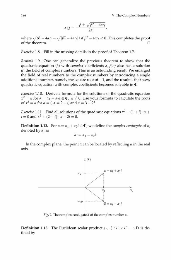
186 V The Complex Numbers
x1,2 =−β±
√β2 − 4αγ
2α,
where√
β2 − 4αγ =√|β2 − 4αγ| i if β2− 4αγ < 0. This completes the proof
of the theorem. ut
Exercise 1.8. Fill in the missing details in the proof of Theorem 1.7.
Remark 1.9. One can generalize the previous theorem to show that thequadratic equation (3) with complex coefficients α, β, γ also has a solutionin the field of complex numbers. This is an astounding result. We enlargedthe field of real numbers to the complex numbers by introducing a singleadditional number, namely the square root of−1, and the result is that everyquadratic equation with complex coefficients becomes solvable in C.
Exercise 1.10. Derive a formula for the solutions of the quadratic equationx2 = α for α = α1 + α2i ∈ C, α 6= 0. Use your formula to calculate the rootsof x2 = α for α = i, α = 2 + i, and α = 3− 2i.
Exercise 1.11. Find all solutions of the quadratic equations x2 + (1 + i) · x +i = 0 and x2 + (2− i) · x− 2i = 0.
Definition 1.12. For α = α1 + α2i ∈C, we define the complex conjugate of α,denoted by α, as
α := α1 − α2i.
In the complex plane, the point α can be located by reflecting α in the realaxis.
//R
OO Ri
;; α = α1 + α2i
α1
α2i
�
_
-α2i ##α = α1 − α2i
Fig. 2. The complex conjugate α of the complex number α.
Definition 1.13. The Euclidean scalar product 〈 · , · 〉 : C×C −→ R is de-fined by

2. Complex Numbers of Modulus 1 and the Special Orthogonal Group 187
〈α, β〉 := Re(α · β) = α1β1 + α2β2,
where α = α1 + α2i, β = β1 + β2i ∈C. The absolute value, or modulus, |α| of αis given by
|α| :=√
α · α =√
α21 + α2
2.
Exercise 1.14.(a) Prove that for all α, β ∈C, one has the product rule |α · β| = |α| · |β|.(b) Use part (a) of this exercise to prove the following: if each of two natural
numbers can be represented as the sum of the squares of two naturalnumbers, then the product of these two numbers can also be representedas the sum of the squares of two natural numbers.
Remark 1.15. Using the previous definition, the multiplicative inverse of 0 6=α ∈C can be written in the form
α−1 =α
|α|2 .
Moreover, one can easily check that the modulus function | · | has the prop-erties of a norm. It turns out that the field (C,+, ·) is complete with respectto this norm.
2. Complex Numbers of Modulus 1 and the Special Orthogonal Group
In this section, we are going to identify the set of complex numbers of unitmodulus with the special orthogonal group.
We begin by considering the noncommutative ring (M2(R), +, ·), whichconsists of all 2× 2 matrices with real entries,
M2(R) :={
A =
(α1 α2α3 α4
) ∣∣∣∣α1, α2, α3, α4 ∈R}
,
together with matrix addition and multiplication as it has been defined inExample 2.4 (iv) of Chapter III. We denote the unit element of M2(R) by
E :=(
1 00 1
).
If A =( α1 α2
α3 α4
)∈M2(R), then the transpose of A, denoted by At, is given by
At :=(
α1 α3α2 α4
)∈M2(R).
Definition 2.1. We define

188 V The Complex Numbers
S1 := {α ∈C | |α| = 1}
to be the set of all complex numbers of modulus 1.
Remark 2.2. The set S1 is a subgroup of the group (C \ {0}, ·).
Exercise 2.3. Verify the assertion of Remark 2.2.
In the following, we shall identify the field of complex numbers with asubring of the noncommutative ring (M2(R), +, ·).
Lemma 2.4. The mapping f : (C, +, ·) −→ (M2(R), +, ·) defined by
α = α1 + α2i 7→(
α1 α2−α2 α1
)is an injective ring homomorphism. The image
C := im( f ) ={(
α1 α2−α2 α1
) ∣∣∣∣α1, α2 ∈R}
is a field. In particular, f induces the isomorphism C∼= C.
Proof. We begin by proving that f is an injective ring homomorphism. Letα = α1 + α2i ∈C and β = β1 + β2i ∈C. We obtain
f (α + β) = f ((α1 + β1) + (α2 + β2)i) =(
α1 + β1 α2 + β2−(α2 + β2) α1 + β1
)=
(α1 α2−α2 α1
)+
(β1 β2−β2 β1
)= f (α) + f (β)
and
f (α · β) = f ((α1 · β1 − α2 · β2) + (α1 · β2 + α2 · β1)i)
=
(α1 · β1 − α2 · β2 α1 · β2 + α2 · β1−(α1 · β2 + α2 · β1) α1 · β1 − α2 · β2
)=
(α1 α2−α2 α1
)·(
β1 β2−β2 β1
)= f (α) · f (β).
Since we have ker( f ) = {0}, we have shown that f is an injective ring ho-momorphism. The image of f is the set
C = im( f ) ={(
α1 α2−α2 α1
) ∣∣∣∣α1, α2 ∈R}
.
By Lemma 3.4 of Chapter III, C is in fact a subring of (M2(R), +, ·). Finally,it follows from the homomorphism theorem for rings that we have the iso-

2. Complex Numbers of Modulus 1 and the Special Orthogonal Group 189
morphismC=C/ker( f ) ∼= im( f ) = C.
But since C is a field, C must also be a field, as asserted. ut
Exercise 2.5. Show that there are infinitely many subrings of (M2(R), +, ·)that are isomorphic to C.
Definition 2.6. The orthogonal group O2(R) is defined by
O2(R) := {A ∈M2(R) | A · At = E}.
The special orthogonal group SO2(R) is defined by
SO2(R) := {A ∈O2(R) | det(A) = 1}.
Remark 2.7. The orthogonal group (O2(R), ·) is a group whose operation ismatrix multiplication. The special orthogonal group SO2(R) is a subgroup,indeed a normal subgroup, of (O2(R), ·).
Exercise 2.8. Show that we have det(A) =±1 for A ∈O2(R), and verify theassertions in Remark 2.7.
Theorem 2.9. We have the group isomorphism
(S1, ·) ∼= (SO2(R), ·).
Proof. We note first that for an arbitrary matrix
A =
(α1 α2−α2 α1
)∈ C,
we have the equalities det(A) = α21 + α2
2 and
A · At =
(α1 α2−α2 α1
)·(
α1 −α2α2 α1
)=
(α2
1 + α22 0
0 α21 + α2
2
)= det(A) · E.
If we now have α = α1 + α2i ∈S1, that is, |α|= 1, then it follows that |α|2 =α2
1 + α22 = 1, and we therefore obtain under the mapping f from Lemma 2.4,
for
A = f (α) = f (α1 + α2i) =(
α1 α2−α2 α1
),
the equalities det(A) = α21 + α2
2 = 1 and A · At = det(A) · E = E. This provesthat A ∈ SO2(R). Thus the mapping f induces an injective group homomor-phism g := f |S1 : S1 −→ SO2(R) with image

190 V The Complex Numbers
im(g) ={
A ∈ C∣∣ det(A) = 1
}⊆ SO2(R).
To prove the surjectivity of g, we have to prove that SO2(R)⊆ im(g). To thisend, let
B :=(
α1 α2α3 α4
)∈ SO2(R).
We then have B · Bt = E, whence also B−1 = Bt. Since det(B) = 1, we havealso
B−1 =
(α4 −α2−α3 α1
).
We must therefore have α4 = α1 and α3 = −α2, which proves that B ∈ C.Since det(B) = 1, it then follows that
SO2(R) ⊆{
A ∈ C∣∣ det(A) = 1
}= im(g).
This completes the proof. ut
Corollary 2.10. Every complex number α ∈C \ {0} can be represented uniquelyin the form
α = |α| · (cos(ϕ) + i sin(ϕ)) (4)
for some ϕ ∈ [0,2π).
Proof. The proof of Theorem 2.9 shows in particular that every matrix A ∈SO2(R) can be represented in the form
A =
(α1 α2−α2 α1
)with α1, α2 ∈ R, where we have the relation α2
1 + α22 = 1. We must also
have α1, α2 ∈ [−1,1], and so there exists a uniquely determined ϕ ∈ [0,2π)with α1 = cos(ϕ) and α2 = sin(ϕ). Since we have α/|α| ∈ S1, there exists auniquely determined ϕ ∈ [0,2π) with
α
|α| = cos(ϕ) + i sin(ϕ),
from which the assertion of the corollary follows. ut
Remark 2.11. The representation (4) is called the polar-coordinate representa-tion of the complex number α. Using this representation, one can prove theimportant fact that it is possible to extract the kth root of a complex numberα for every k ∈ N, k > 1. We saw this earlier, in Exercise 1.10, for the casek = 2.

3. The Fundamental Theorem of Algebra 191
Exercise 2.12. Prove de Moivre’s theorem: Let α ∈ C \ {0} be represented inpolar coordinates as α = |α| · (cos(ϕ) + i sin(ϕ)). Then we have the equality
αm/n = |α|m/n ·(
cos(m
nϕ)+ i sin
(mn
ϕ))
for m, n ∈N and n 6= 0.
3. The Fundamental Theorem of Algebra
In this section, we shall give an elementary proof of the fundamental the-orem of algebra. In doing so, we shall use without proof the well-knownfact from calculus that a continuous real function of one or several variablesdefined on a closed, bounded set assumes a minimum value.
Theorem 3.1 (Fundamental theorem of algebra). Every polynomial
f (X) = αnXn + αn−1Xn−1 + · · ·+ α1X + α0
of degree n > 0 with complex coefficients α0, . . . , αn has at least one root in the fieldC. As a result, the polynomial f can be decomposed in C into linear factors. Thatis, there exist complex numbers ζ1, . . . , ζn such that
f (X) = αn · (X− ζ1) · · · (X− ζn).
Proof. Without loss of generality, we shall assume that αn = 1, and we write
f (X) = Xn + g(X),
with g(X) := αn−1Xn−1 + · · · + α1X + α0. We begin by showing that thereexists a complex number ζ0 ∈C such that
| f (ζ0)| ≤ | f (ζ)|
for all ζ ∈C. For the real number
r := 1 + |αn−1|+ · · ·+ |α1|+ |α0| ∈R,
we obtain for all ζ ∈Cwith |ζ| > r ≥ 1 the estimate
|g(ζ)| ≤ |ζn−1| ·(|αn−1|+ · · ·+
|α1||ζn−2| +
|α0||ζn−1|
)≤ |ζn−1| ·
(|αn−1|+ · · ·+ |α1|+ |α0|
)≤ |ζ|n−1 · (r− 1) < |ζ|n−1 · (|ζ| − 1).
This yields for ζ ∈Cwith |ζ| > r ≥ 1 the inequality

192 V The Complex Numbers
| f (ζ)| = |ζn + g(ζ)| ≥ |ζn| − |g(ζ)|≥ |ζ|n − |ζ|n−1 · (|ζ| − 1) = |ζ|n−1 ≥ |ζ| > r. (5)
To obtain an estimate for ζ ∈ C with |ζ| ≤ r, we identify C with the Carte-sian plane, as in Remark 1.4. By decomposing the (complex) variable X andthereby also f (X) into its real and imaginary parts, we may view f as a con-tinuous real mapping from R2 to R2. But then the function | f | defined onthe closed disk {ζ ∈C | |ζ| ≤ r} ⊆R2 must attain a minimum. That is, thereexists ζ0 ∈C, |ζ0| ≤ r, such that
| f (ζ0)| ≤ | f (ζ)| (6)
for all ζ ∈Cwith |ζ| ≤ r. In particular, we must have
| f (ζ0)| ≤ | f (0)| = |α0| < r. (7)
In sum, the estimates (5), (6), and (7), prove that the inequality | f (ζ0)| ≤| f (ζ)| holds for all ζ ∈C, as asserted.
We show now that ζ0 is a zero of f (X). Without loss of generality, we mayassume that ζ0 = 0, since otherwise, we could as well consider the polyno-mial f (X + ζ0). We shall carry out a proof by contradiction and assume thatf (0) = α0 6= 0. If k ∈ {1, . . . ,n} is minimal with αk 6= 0, then we can write
f (X) = Xk+1 · h(X) + αkXk + α0
for some polynomial h(X). Since we may extract the kth root of any complexnumber, there exists a complex number β ∈C, β 6= 0, such that
βk = −α0
αk.
We then define, for t ∈R, the function
q(t) := tβk+1 · h(tβ), i.e., f (tβ) = tk · q(t) + αktkβk + α0.
Since q(0) = 0 and the function |q(t)| is continuous, there exists t0 ∈R with0 < t0 < 1 such that
|q(t0)| < |α0|.We thereby obtain the estimate
| f (t0β)| =∣∣∣tk
0 · q(t0)− α0tk0 + α0
∣∣∣ ≤ ∣∣∣tk0 · q(t0)
∣∣∣+ |α0|(
1− tk0
)< tk
0 · |α0|+ |α0|(
1− tk0
)= |α0| = | f (0)|.

4. Algebraic and Transcendental Numbers 193
But this contradicts that | f | assumes its minimum at ζ0 = 0. Our assumptionmust therefore be false, and we must have f (0) = 0. That is, the polynomialf (X) has at least the zero ζ0 ∈C. ut
Remark 3.2. A field K in which the analogue of the fundamental theorem ofalgebra holds is said to be algebraically closed. Thus the field C of complexnumbers is algebraically closed.
4. Algebraic and Transcendental Numbers
Definition 4.1. A complex number α is said to be algebraic of degree n if it isthe root of a polynomial
f (X) = anXn + an−1Xn−1 + · · ·+ a1X + a0 (8)
of degree n > 0 with integer coefficients a0, . . . , an but is not a root of such apolynomial of lower degree.
We denote the set of algebraic numbers byQ.
Remark 4.2. The set Q of algebraic numbers contains all rational numbers,since every rational number r = m/n (m, n ∈ Z; n > 0) is algebraic of de-gree 1, namely as the root of the polynomial
f (X) = nX−m.
This means in addition that an algebraic number of degree n > 1 cannot berational.
Example 4.3. The irrational number√
2 is algebraic of degree 2, since it is aroot of the polynomial f (X) = X2 − 2.
Exercise 4.4. Let p be a prime number. Show that√
p is algebraic of degree 2.
Theorem 4.5. The setQ of algebraic numbers is countable.
Proof. To prove that the set of algebraic numbers is countable, it suffices toprove that the set (8) of polynomials is countable, since each polynomial hasonly finitely many roots. For a fixed degree n > 0, there are countably manypossibilities for each of the coefficients. Therefore, there are countably manypolynomials of degree n with integer coefficients. Since there are only count-ably many choices for the degree n of a polynomial, it follows that there arecountably many polynomials of positive degree with integer coefficients.This proves the theorem. ut
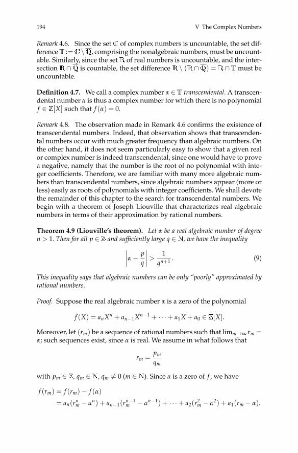
194 V The Complex Numbers
Remark 4.6. Since the setC of complex numbers is uncountable, the set dif-ference T :=C\Q, comprising the nonalgebraic numbers, must be uncount-able. Similarly, since the setR of real numbers is uncountable, and the inter-section R ∩Q is countable, the set difference R \ (R ∩Q) =R ∩T must beuncountable.
Definition 4.7. We call a complex number α ∈ T transcendental. A transcen-dental number α is thus a complex number for which there is no polynomialf ∈ Z[X] such that f (α) = 0.
Remark 4.8. The observation made in Remark 4.6 confirms the existence oftranscendental numbers. Indeed, that observation shows that transcenden-tal numbers occur with much greater frequency than algebraic numbers. Onthe other hand, it does not seem particularly easy to show that a given realor complex number is indeed transcendental, since one would have to provea negative, namely that the number is the root of no polynomial with inte-ger coefficients. Therefore, we are familiar with many more algebraic num-bers than transcendental numbers, since algebraic numbers appear (more orless) easily as roots of polynomials with integer coefficients. We shall devotethe remainder of this chapter to the search for transcendental numbers. Webegin with a theorem of Joseph Liouville that characterizes real algebraicnumbers in terms of their approximation by rational numbers.
Theorem 4.9 (Liouville’s theorem). Let α be a real algebraic number of degreen > 1. Then for all p ∈ Z and sufficiently large q ∈N, we have the inequality∣∣∣∣α− p
q
∣∣∣∣ > 1qn+1 . (9)
This inequality says that algebraic numbers can be only “poorly” approximated byrational numbers.
Proof. Suppose the real algebraic number α is a zero of the polynomial
f (X) = anXn + an−1Xn−1 + · · ·+ a1X + a0 ∈ Z[X].
Moreover, let (rm) be a sequence of rational numbers such that limm→∞ rm =α; such sequences exist, since α is real. We assume in what follows that
rm =pm
qm
with pm ∈ Z, qm ∈N, qm 6= 0 (m ∈N). Since α is a zero of f , we have
f (rm) = f (rm)− f (α)
= an(rnm − αn) + an−1(rn−1
m − αn−1) + · · ·+ a2(r2m − α2) + a1(rm − α).

4. Algebraic and Transcendental Numbers 195
Division by (rm − α) yields
f (rm)
rm − α= an(rn−1
m + rn−2m α + · · ·+ rmαn−2 + αn−1) + · · ·
+ a3(r2m + rmα + α2) + a2(rm + α) + a1.
Since limm→∞ rm = α, there exists N ∈N such that
|rm − α| < 1
for all m ≥ N. We therefore have |rm| < |α| + 1 for all m ≥ N. Using thetriangle inequality, we thereby obtain for sufficiently large m the estimate∣∣∣∣ f (rm)
rm − α
∣∣∣∣ < n · |an| · (|α|+ 1)n−1 + · · ·+ 3 · |a3| · (|α|+ 1)2
+ 2 · |a2| · (|α|+ 1) + |a1| =: M.
We note that the positive real number M is determined solely by α. In par-ticular, it is independent of m. We now choose the index m sufficiently largethat for the denominator qm of the approximating fraction rm = pm/qm, wehave qm > M. This leads to∣∣∣∣ f (rm)
rm − α
∣∣∣∣ < qm ⇐⇒ |α− rm| >| f (rm)|
qm. (10)
Now, the rational numbers rm cannot be zeros of the polynomial f , since wecould then factor out the linear factor (X− rm) from f , revealing α as a zeroof a polynomial of degree less than n, which cannot be the case. In otherwords, we have
| f (rm)| =∣∣∣∣ an pn
m + an−1 pn−1m qm + · · ·+ a1 pmqn−1
m + a0qnm
qnm
∣∣∣∣ 6= 0. (11)
Since the numerator in (11) is a nonzero integer, its absolute value must beat least 1. Using the estimates (10) and (11), we finally obtain∣∣∣∣α− pm
qm
∣∣∣∣ > | f (rm)|qm
≥ 1qn
m· 1
qm=
1qn+1
m.
This completes the proof of Liouville’s theorem. ut
Remark 4.10. With Liouville’s theorem at our disposal, we can now findtranscendental numbers as follows. Assume that a given real number α isalgebraic of degree n > 0. Showing that the inequality (9) cannot hold meansthat α must be transcendental. Standard examples of such numbers are realnumbers whose decimal expansions contain blocks of zeros of rapidly in-
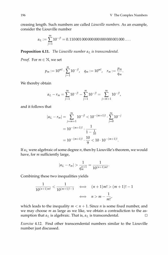
196 V The Complex Numbers
creasing length. Such numbers are called Liouville numbers. As an example,consider the Liouville number
αL :=∞
∑j=1
10−j! = 0.110001000000000000000001000 . . . .
Proposition 4.11. The Liouville number αL is transcendental.
Proof. For m ∈N, we set
pm := 10m! ·m
∑j=1
10−j!, qm := 10m!, rm :=pm
qm.
We thereby obtain
αL − rm =∞
∑j=1
10−j! −m
∑j=1
10−j! =∞
∑j=m+1
10−j!,
and it follows that
|αL − rm| =∞
∑j=m+1
10−j! < 10−(m+1)! ·∞
∑j=0
10−j
= 10−(m+1)! · 11− 1
10
= 10−(m+1)! · 109
< 10 · 10−(m+1)!.
If αL were algebraic of some degree n, then by Liouville’s theorem, we wouldhave, for m sufficiently large,
|αL − rm| >1
qn+1m
=1
10(n+1)m!.
Combining these two inequalities yields
110(n+1)m!
<1
10(m+1)!−1⇐⇒ (n + 1)m! > (m + 1)!− 1
⇐⇒ n > m− 1m!
,
which leads to the inequality m < n + 1. Since n is some fixed number, andwe may choose m as large as we like, we obtain a contradiction to the as-sumption that αL is algebraic. That is, αL is transcendental. ut
Exercise 4.12. Find other transcendental numbers similar to the Liouvillenumber just discussed.

5. The Transcendence of e 197
A transcendental number much better known than the Liouville numbersis Euler’s number e, the base of the natural logarithm, whose transcendencewe shall prove in the following section.
5. The Transcendence of e
Definition 5.1. Euler’s number e is defined by the infinite series
∞
∑j=0
1j!
.
Remark 5.2. The number e thus begins with the decimal expansion e =2.718281828459 . . . . It is the base of the exponential function, defined by
eX :=∞
∑j=0
X j
j!.
For real values of X, the exponential function is strictly monotonically in-creasing, and it assumes only positive values. It is infinitely differentiableand is equal to all its derivatives.
Before we prove that e is transcendental, we shall begin by showing thate is irrational.
Lemma 5.3. The number e is irrational.
Proof. We begin by assuming for the sake of obtaining a contradiction thate is rational, that is, that e = m
n for m, n ∈ N and n > 0. We now choosea natural number k > 2 and consider the following decomposition of thedefining series for e:
mn= e = sk + rk with sk :=
k
∑j=0
1j!
, rk :=∞
∑j=k+1
1j!
. (12)
We now estimate
rk =1
(k + 1)!
(1 +
1k + 2
+1
(k + 2)(k + 3)+ · · ·
)<
1(k + 1)!
∞
∑j=0
1(k + 2)j =
1(k + 1)!
· 11− 1
k+2
<2
(k + 1)!.

198 V The Complex Numbers
Multiplying (12) by k!, yields
mn· k! = e · k! = sk · k! + rk · k! ,
that is,mn· k!− sk · k! = rk · k! .
For k > n, the left-hand side of this last equation represents an integer,whereas on the right-hand side, since k > 2, we have
0 < rk · k! <2k!
(k + 1)!=
2k + 1
< 1.
This contradiction proves that our assumption of the rationality of e wasfalse. ut
Remark 5.4. In the following proof of the transcendence of e, we shall at-tempt to approximate the exponential function by a polynomial. We shalluse the fact that the exponential function is characterized as the unique dif-ferentiable function g :R−→R satisfying the following two properties:(1) g′(X) = g(X) (X ∈R),(2) g(0) = 1.This can be seen as follows. We consider the differentiable function e−X g(X),whose derivative is given by(
e−X g(X))′= e−X g′(X)− e−X g(X) = 0.
From this, we see that the function e−X g(X) is constant onR. Since e−0g(0) =1, this constant must be equal to 1, from which it follows that g(X) = eX .For approximating the exponential function, we shall attempt to construct apolynomial whose derivative is more or less equal to the polynomial itselfand whose value at the point X = 0 is equal to 1.
Theorem 5.5. The number e is transcendental.
Proof. We break the proof into six steps.Step 1: proof strategy. We shall assume the opposite of the statement of
the theorem, namely that e is algebraic of degree m, that is, that there exista0, . . . , am ∈ Zwith a0 6= 0 and am 6= 0 such that
amem + am−1em−1 + · · ·+ a1e + a0 = 0.
We sketch in this first step how we are going to manage to obtain a con-tradiction. We shall assume that there exists a polynomial H ∈ Q[X] thatsatisfies the following four properties:(i) H(0) 6= 0,

5. The Transcendence of e 199
(ii) H(j) ∈ Z (j = 0, . . . , m),(iii) ∑m
j=0 aj H(j) 6= 0,(iv)
∣∣∑mj=1 aj
(H(0)ej − H(j)
)∣∣ < 1.In the following steps, we shall construct such a polynomial. We then set
c :=m
∑j=0
aj H(j), (13)
ε j := H(0)ej − H(j) (j = 0, . . . , m), (14)
σ :=m
∑j=1
ajε j. (15)
Properties (ii) and (iii) show that c in (13) is a nonzero integer. Using prop-erty (i), we can transform (14) to
ej =H(j)H(0)
+ε j
H(0)(j = 0, . . . , m);
this can be interpreted as an approximation to the powers ej of e (j = 0, . . . ,m)by the polynomial H(X)/H(0). From property (iv), we see that for σ in (15),we have |σ| < 1. Putting everything together, we have
0 =m
∑j=0
ajej
=m
∑j=0
aj
(H(j)H(0)
+ε j
H(0)
)
=1
H(0)
m
∑j=0
ajH(j) +1
H(0)
m
∑j=0
ajε j
=c
H(0)+
σ
H(0).
After multiplying the last equation by H(0) on both sides and rearranging,we end up with the equation
c = −σ, that is, |c| = |σ|. (16)
But now we have c ∈ Z and c 6= 0; that is, |c| ≥ 1. But we also have |σ| <1. Therefore, (16) is impossible. This gives the desired contradiction to theassumption of the algebraicity of e. We conclude, then, that the number emust be transcendental.
Step 2: definition of H. We choose an arbitrary prime number p, which weshall specify more precisely later. We also define an auxiliary polynomial

200 V The Complex Numbers
f (X) := Xp−1(X− 1)p(X− 2)p · · · (X−m)p,
of degree N = p− 1+ m · p. From it, we construct another auxiliary polyno-mial, namely
F(X) := f (X) + f ′(X) + · · ·+ f (N)(X).
Since the (N + 1)st derivative of f vanishes identically, we have
F′(X) = f ′(X) + f ′′(X) + · · ·+ f (N)(X) = F(X)− f (X).
The derivative of the polynomial F would now more or less approximateF itself on the interval [0, m] if f were in some sense small there. To get ahandle on the size, we have to estimate the auxiliary polynomial f on theinterval [0, m]. We observe first that
|X(X− 1) · · · (X−m)| ≤ mm+1 (X ∈ [0, m]).
Setting M := mm+1 gives us the estimate
max0≤X≤m
| f (X)| ≤ Mp.
We see that f is not small on the interval [0, m]. For this reason, we consider,instead of F, the polynomial
H(X) :=F(X)
(p− 1)!.
These considerations lead to the equation
H′(X) = H(X)− f (X)
(p− 1)!;
and we have also
max0≤X≤m
∣∣∣∣ f (X)
(p− 1)!
∣∣∣∣ ≤ Mp
(p− 1)!.
Since the quantity Mp/(p − 1)! can be made arbitrarily small by choos-ing the prime p sufficiently large, we see that the normalized polynomialH(X)/H(0) approximates the exponential function eX well on the interval[0, m] if p is chosen sufficiently large.
Step 3: H satisfies property (i). We have
f (X) =N
∑k=0
bkXk
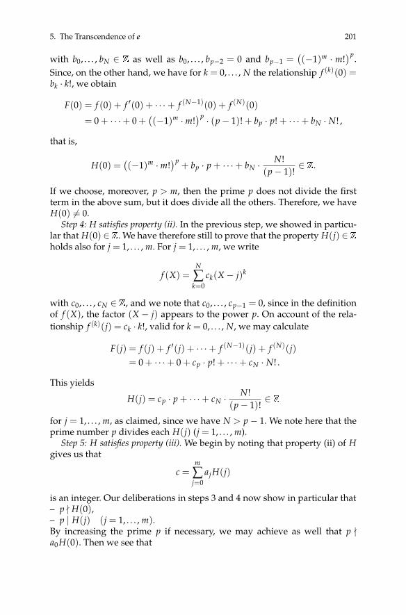
5. The Transcendence of e 201
with b0, . . . , bN ∈ Z as well as b0, . . . , bp−2 = 0 and bp−1 =((−1)m · m!
)p.Since, on the other hand, we have for k = 0, . . . , N the relationship f (k)(0) =bk · k!, we obtain
F(0) = f (0) + f ′(0) + · · ·+ f (N−1)(0) + f (N)(0)
= 0 + · · ·+ 0 +((−1)m ·m!
)p · (p− 1)! + bp · p! + · · ·+ bN · N! ,
that is,
H(0) =((−1)m ·m!
)p+ bp · p + · · ·+ bN ·
N!(p− 1)!
∈ Z.
If we choose, moreover, p > m, then the prime p does not divide the firstterm in the above sum, but it does divide all the others. Therefore, we haveH(0) 6= 0.
Step 4: H satisfies property (ii). In the previous step, we showed in particu-lar that H(0) ∈Z. We have therefore still to prove that the property H(j) ∈Zholds also for j = 1, . . . , m. For j = 1, . . . , m, we write
f (X) =N
∑k=0
ck(X− j)k
with c0, . . . , cN ∈ Z, and we note that c0, . . . , cp−1 = 0, since in the definitionof f (X), the factor (X − j) appears to the power p. On account of the rela-tionship f (k)(j) = ck · k!, valid for k = 0, . . . , N, we may calculate
F(j) = f (j) + f ′(j) + · · ·+ f (N−1)(j) + f (N)(j)= 0 + · · ·+ 0 + cp · p! + · · ·+ cN · N! .
This yields
H(j) = cp · p + · · ·+ cN ·N!
(p− 1)!∈ Z
for j = 1, . . . , m, as claimed, since we have N > p− 1. We note here that theprime number p divides each H(j) (j = 1, . . . , m).
Step 5: H satisfies property (iii). We begin by noting that property (ii) of Hgives us that
c =m
∑j=0
aj H(j)
is an integer. Our deliberations in steps 3 and 4 now show in particular that– p - H(0),– p | H(j) (j = 1, . . . , m).By increasing the prime p if necessary, we may achieve as well that p -a0H(0). Then we see that

202 V The Complex Numbers
p -(a0H(0) + a1H(1) + · · ·+ amH(m)
)⇐⇒ p - c.
Thus c is an integer that is not divisible by p; in particular, we have c 6= 0.Step 6: H satisfies property (iv). For t ∈R, we have the differential equation
ddt(
F(0)− F(t)e−t) = F(t)e−t − F′(t)e−t =(
F(t)− F′(t))e−t = f (t)e−t.
Applying the fundamental theorem of calculus to X ∈R yields
F(0)− F(X)e−X =∫ X
0f (t)e−t dt.
On dividing by (p− 1)!, we obtain at the point X = j ∈ {1, . . . , m} the equal-ity
H(0)− H(j)e−j =1
(p− 1)!
∫ j
0f (t)e−t dt .
From this, we obtain the estimate∣∣∣H(0)− H(j)e−j∣∣∣ ≤ 1
(p− 1)!max
0≤X≤m| f (X)|
∫ j
0e−t dt
≤ Mp
(p− 1)!(1− e−j)
≤ Mp
(p− 1)!.
On multiplying by ej, we obtain∣∣∣H(0)ej − H(j)∣∣∣ ≤ Mp
(p− 1)!ej,
whence ∣∣∣∣∣ m
∑j=1
ajε j
∣∣∣∣∣ =∣∣∣∣∣ m
∑j=1
aj
(H(0)ej − H(j)
)∣∣∣∣∣ ≤ Mp
(p− 1)!
m
∑j=1|aj|ej.
Since the sum ∑mj=1 |aj|ej is independent of p, and we can make the quantity
Mp/(p− 1)! arbitrarily small by choosing p sufficiently large, we obtain fora suitable choice of the prime p the estimate
|σ| =∣∣∣∣∣ m
∑j=1
ajε j
∣∣∣∣∣ < 1.
We have thereby finally shown that the polynomial H satisfies property (iv),which ensures the existence of the polynomial H having properties (i)–(iv)

5. The Transcendence of e 203
postulated in the first step. This completes the proof of the transcendenceofe. ut
Remark 5.6. Even more spectacular than the proof of the transcendence ofe is the proof of the transcendence of π. This result shows in particular thatthe number π is not constructible with straightedge and compass, which inturn proves the impossibility of squaring the circle. The proof of the tran-scendence of π follows along some of the same lines as that of the transcen-dence of e. However, at a certain point, it is necessary to bring in some of thetools of complex analysis, in particular Cauchy’s integral theorem, whichwould take us beyond the scope of this book.
Example 5.7. We will close out the main part of this chapter by presentingtwo examples that illustrate how the polynomial H constructed in the proofof Theorem 5.5 can be used to obtain good approximations to the number e.Recall from that theorem that
H(X) =F(X)
(p− 1)!
and that H(X)/H(0) = F(X)/F(0) is a “good” approximation to the expo-nential function eX on the interval [0, m]. To obtain an approximation to thenumber e itself, we consider the quotient F(1)/F(0).
(i) We choose m = 1, p = 3 and calculate
f (X) = X2(X− 1)3,
F(X) = X5 + 2X4 + 11X3 + 32X2 + 64X + 64,F(0) = 64, F(1) = 174.
We thereby obtainF(1)F(0)
= 2.71875,
which is already a fairly good approximation to e.(ii) We choose m = 2, p = 5 and calculate
f (X) = X4(X− 1)5(X− 2)5,
F(X) = X14 − X13 + 87X12 + 654X11 + · · ·+ 29141344128,F(0) = 29141344128, F(1) = 79214386200.
We now obtainF(1)F(0)
= 2.718281828458561 . . . ,
which agrees with the decimal expansion of e to ten decimal places.

204 V The Complex Numbers
Exercise 5.8. Compute in the way described above further approximationsto e.
E. Zeros of Polynomials: The Search for Solution Formulas
The point of departure for this appendix is the fundamental theorem of al-gebra, which we proved in this chapter as Theorem 3.1. The theorem saysthat every polynomial f (X) of positive degree n with complex coefficients,that is, f ∈ C[X], has all of its zeros in C.
Knowing as we do that the zeros of every quadratic polynomial can beexpressed through an explicit formula involving the four arithmetic opera-tions and the extraction of roots, the question naturally arises whether sim-ilar formulas exist for polynomials of higher degree. It is this question andits consequences that we wish to explore in this appendix. And as we do,we shall come to realize that efforts to resolve this problem extend to activeresearch in number theory today.
E.1 Zeros of Polynomials of Degree n ≤ 4
The zeros of linear and quadratic polynomials with complex coefficients areeasily determined. In the quadratic case, we presented the solution formulasin the proof of Theorem 1.7, in connection with which the reader should alsotake note of Remark 1.9.
We now turn to determining the zeros of an arbitrary third-degree poly-nomial f (X) with complex coefficients. First of all, we may, without loss ofgenerality, assume that f (X) has the form
f (X) = X3 + βX + γ (17)
with β,γ ∈ C. Namely, if f (X) = X3 + α′X2 + β′X + γ′, then one can obtainthe desired form (17) by means of the substitution X 7→ X− α′/3, known asthe Tschirnhaus transformation.
If we now decompose a zero ζ ∈ C of the polynomial (17) as ζ = ξ + η,we obtain the equation
3ξηζ + ξ3 + η3 = ζ3 = −βζ − γ.
Comparing coefficients yields
ξ3 + η3 = −γ and ξ · η = − β
3, whence ξ3 · η3 = −
(β
3
)3

E. Zeros of Polynomials: The Search for Solution Formulas 205
and thus ξ3 and η3 can be viewed as the two zeros of the quadratic polyno-mial
X2 + γX− β3
27.
This is, incidentally, the assertion of Viète’s theorem. This polynomial iscalled the quadratic resolvent of the cubic polynomial (17). The first zero of(17) thus takes the form
ζ1 =3
√−γ
2+
√γ2
4+
β3
27+
3
√−γ
2−√
γ2
4+
β3
27.
The other two zeros of the cubic polynomial (17) can be obtained with thehelp of a complex third root of unity ε, that is, a complex number ε satisfyingε3 = 1, for example,
ε = −12+
√3
2i.
Taking into account the relation ξη = −β/3, we obtain
ζ2 = ε3
√−γ
2+
√γ2
4+
β3
27+ ε2 3
√−γ
2−√
γ2
4+
β3
27,
ζ3 = ε2 3
√−γ
2+
√γ2
4+
β3
27+ ε
3
√−γ
2−√
γ2
4+
β3
27.
These solution formulas first appeared in Girolamo Cardano’s 1545 bookArs Magna and are therefore known as Cardano’s formulas; they had beendiscovered earlier by Niccolò Tartaglia. Altogether, we may state that in thecase of a cubic polynomial, its zeros can be expressed in terms of (squareand cube) roots of the polynomial’s coefficients.
We now turn our attention to determining the zeros of an arbitrary fourth-degree polynomial f (X) with complex coefficients. In analogy to the cubiccase, we may assume without loss of generality that f (X) is of the form
f (X) = X4 + βX2 + γX + δ, (18)
with β,γ,δ ∈ C. As in the previous case, the problem of finding the zerosof (18) will be reduced to determining the zeros of a polynomial of lowerdegree, the so-called cubic resolvent, which is given by the cubic polynomial
X3 + 2βX2 + (β2 − 4δ)X− γ2 . (19)
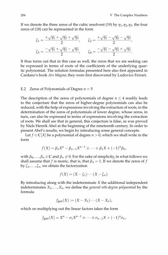
206 V The Complex Numbers
If we denote the three zeros of the cubic resolvent (19) by η1,η2,η3, the fourzeros of (18) can be represented in the form
ζ1 =+√
η1 +√
η2 +√
η3
2, ζ2 =
+√
η1 −√
η2 −√η3
2,
ζ3 =−√η1 +
√η2 −√η3
2, ζ4 =
−√η1 −√
η2 +√
η3
2.
It thus turns out that in this case as well, the zeros that we are seeking canbe expressed in terms of roots of the coefficients of the underlying quar-tic polynomial. The solution formulas presented here also first appeared inCardano’s book Ars Magna; they were first discovered by Ludovico Ferrari.
E.2 Zeros of Polynomials of Degree n = 5
The description of the zeros of polynomials of degree n ≤ 4 readily leadsto the conjecture that the zeros of higher-degree polynomials can also bereduced, with the help of expressions involving the extraction of roots, to thedetermination of the zeros of polynomials of lower degree, whose zeros, inturn, can also be expressed in terms of expressions involving the extractionof roots. We shall see that in general, this conjecture is false, as was provedby Niels Henrik Abel at the beginning of the nineteenth century. In order topresent Abel’s results, we begin by introducing some general concepts.
Let f ∈ C[X] be a polynomial of degree n > 0, which we shall write in theform
f (X) = βnXn − βn−1Xn−1 ± · · · ± β1X + (−1)nβ0 ,
with β0, . . . , βn ∈C and βn 6= 0. For the sake of simplicity, in what follows weshall assume that f is monic, that is, that βn = 1. If we denote the zeros of fby ζ1, . . . ,ζn, we obtain the factorization
f (X) = (X− ζ1) · · · (X− ζn).
By introducing along with the indeterminate X the additional independentindeterminates X1, . . . , Xn, we define the general nth-degree polynomial by theformula
fgen(X) := (X− X1) · · · (X− Xn),
which on multiplying out the linear factors takes the form
fgen(X) = Xn − σ1Xn−1 ± · · · ± σn−1X + (−1)nσn ,
E. Zeros of Polynomials: The Search for Solution Formulas 207
where the coefficients σ1, . . . ,σn are given by the elementary symmetric polyno-mials
σ1 = σ1(X1, . . . , Xn) =n
∑j=1
Xj,
σ2 = σ2(X1, . . . , Xn) =n
∑j,k=1j<k
XjXk,
· · ·σn = σn(X1, . . . , Xn) = X1 · · ·Xn .
The coefficients of fgen lie in the field of rational functions in the indetermi-nates σ1, . . . ,σn, that is, in the quotient field Quot(C[σ1, . . . ,σn]) of the polyno-mial ring C[σ1, . . . ,σn], whose elements are quotients of polynomials in theindeterminates σ1, . . . ,σn and which we denote by C(σ1, . . . ,σn). The zeros ofthe polynomial
fgen ∈ C(σ1, . . . ,σn)[X]
lie in the field of rational functions in the indeterminates X1, . . . , Xn, that is,in the field C(X1, . . . , Xn), which contains the field C(σ1, . . . ,σn).
Example E.1. The general polynomial of degree 2 is given by
fgen(X) = (X− X1) · (X− X2)
= X2 − (X1 + X2)X + X1X2
= X2 − σ1X + σ2.
Its coefficients are the elementary symmetric polynomials σ1 = σ1(X1, X2) =X1 + X2 and σ2 = σ2(X1, X2) = X1X2. We therefore have fgen ∈ C(σ1,σ2)[X].The two zeros X1 and X2 of fgen(X) are elements of the field C(X1, X2). Byspecializing σ1 and σ2, that is, by evaluating σ1 and σ2 at particular complexnumbers, one can obtain every monic second-degree polynomial f ∈ C[X].This explains why we call fgen(X) the general polynomial of degree 2.
Definition E.2. Let fgen ∈ C(σ1, . . . ,σn)[X] be the general polynomial of de-gree n. We say that the zeros X1, . . . , Xn can be expressed in terms of radicals ifthere exist m ∈N>0 and polynomials p0, p1, . . . , pm−1, R ∈ C(σ1, . . . ,σn) withR1/m /∈ C(σ1, . . . ,σn) such that every Xj can be represented in the form
Xj = p0 + p1R1/m + p2R2/m + · · ·+ pm−1R(m−1)/m (20)
or more generally as a finite iteration of such expressions. Here the depen-dence of the right-hand side of (20) on the index j (j = 1, . . . ,n) comes into

208 V The Complex Numbers
play, in that various choices of the radical R1/m can be made, which differfrom one another by an mth root of unity.
Example E.3. For the two zeros X1, X2 of the general quadratic polynomialfgen(X) = X2 − σ1X + σ2, one has
X1,2 =σ1 ±
√σ2
1 − 4σ2
2=
σ1
2± 1
2R1/2 ,
with p0 = σ1/2, p1 = 1/2, and R = σ21 − 4σ2 ∈ C(σ1,σ2). Thus the two zeros
X1, X2 of fgen(X) can be expressed in terms of radicals.
Similarly, one can easily see, using the solution formulas given above, thatthe zeros of the general cubic and quartic polynomials can also be expressedin terms of radicals. However, one has the following theorem.
Theorem E.4 (Abel). Let fgen ∈ C(σ1, . . . ,σ5)[X] denote the general polynomialof degree 5. Then the zeros X1, . . . , X5 of fgen(X) cannot be represented in terms ofradicals.
Proof. We shall briefly sketch the idea of the proof. We begin by supposing,in contradiction to the assertion of the theorem, that the zeros of fgen areindeed representable in terms of radicals. Based on that assumption, it turnsout that the zeros X1, . . . , X5 must satisfy an algebraic relation over C, whichcontradicts the assumption that fgen is the general polynomial of degree 5,whose zeros are therefore algebraically independent over C and thereforecan satisfy no polynomial relation over C. ut
E.3 The Bridge to Group Theory: Galois Theory
The negative result given by Abel’s theorem, Theorem E.4, raises the prob-lem of providing a conceptual characterization of the zeros of polynomialswhose coefficients lie in a fixed field K. With this in mind, we again considerthe general polynomial fgen ∈ C(σ1, . . . ,σn)[X] of degree n and observe thatK := C(σ1, . . . ,σn) can be characterized by the fact that K is the field con-structed of all rational functions from E := C(X1, . . . , Xn) that remain invari-ant under permutations of the indeterminates X1, . . . , Xn. This insight arisesfrom the nontrivial fact that a polynomial g ∈ C[X1, . . . , Xn] that remains in-variant under all permutations of the indeterminates X1, . . . , Xn must be apolynomial in the elementary symmetric polynomials σ1, . . . ,σn. This resultcarries over directly to rational functions in the indeterminates X1, . . . , Xnthat are invariant under all permutations of X1, . . . , Xn. We have thereby, ina natural way, associated with the field E and subfield K a characterizinggroup, the nth symmetric group Sn (see Example 2.8 (iv) of Chapter II). This

E. Zeros of Polynomials: The Search for Solution Formulas 209
association is the starting point of Galois theory, whose basic features weshall now present.
Definition E.5. Let K be an arbitrary field. A field E that contains the fieldK is called a field extension of K. The extension E⊇ K is denoted by E/K, andwe say “E over K.” A field extension E of K can be viewed naturally as aK-vector space, and such a field extension is said to be finite over K if E isfinite-dimensional as a K-vector space. We let [E : K] denote the dimensiondimK E and call this number the degree of E over K.
Definition E.6. Let K be an arbitrary field, and E/K a field extension. Wesay that an element α ∈ E is algebraic over K if α is a zero of a polynomialf ∈ K[X]. A field extension E of K is said to be algebraic over K if all of itselements are algebraic over K; we also say that we have an algebraic fieldextension E/K.
Example E.7. For K = Q and E = C, we saw in Section 4 of this chapter thata number α ∈ C is algebraic over Q precisely when α ∈ Q, that is, when αis an algebraic number. In particular, transcendental numbers are not alge-braic over Q. We have therefore that neither C/Q nor R/Q is an algebraicfield extension. We saw, however, in Section 1 of this chapter that C/R is analgebraic and finite field extension of degree [C : R] = dimR C = 2.
Remark E.8. One can see at once that a finite field extension E/K is algebraic,since the [E : K] + 1 powers
1, α, α2, . . . , α[E:K]
of an arbitrary element α ∈ E must be linearly dependent over K, whence αis a zero of a polynomial with coefficients in K.
Remark E.9. If α is a zero of a nontrivial polynomial in the polynomial ringK[X], then there exists a monic polynomial f of minimal degree with α as azero. Such a polynomial f is uniquely determined and is called the minimalpolynomial of α. The existence of such a polynomial f can be seen simplyby considering the set
aα := {g ∈ K[X] | g(α) = 0},
which is obviously a nontrivial ideal of K[X], and indeed, it is a principalideal, since K[X] is a Euclidean domain. That is, aα = ( f ) with f a polynomialof minimal positive degree, which can be made monic. The uniqueness canbe seen at once by applying the Euclidean algorithm. Moreover, one seesthat the minimal polynomial f of α is irreducible over K.
Example E.10. Let K = Q and
210 V The Complex Numbers
E ={
α = a + b√−3 | a,b ∈Q
}.
It is easily verified that E is a field that contains the field K = Q. The field ex-tension E/K is finite over K. Indeed, we have [E : K] = 2, since the elements1 and
√−3 constitute a basis of E over K. And so E is also algebraic over K.
The minimal polynomial of the element α =√−3 is f (X) = X2 + 3.
Remark E.11. In general, we can construct a field extension of K that con-tains the zero α of a polynomial f that is irreducible over K. To this end, weconsider the ring homomorphism ϕ : K[X]→ K[α] given by replacing theindeterminate X with the element α. Since the kernel of the homomorphismϕ is the ideal aα = ( f ), the homomorphism theorem for rings gives us theisomorphism
K[α] ∼= K[X]/( f ).
Since the polynomial f is irreducible over K, the principal ideal ( f ) is aprime ideal, indeed a maximal ideal, which means that the quotient ringK[X]/( f ) is a field. This field is the desired extension of K that contains theelement α. Moreover, our construction shows that the ring K[α] is in fact afield, equal to its field of quotients K(α). It is easy to see that K(α) is a finitefield extension of K and that [K(α) : K] = deg( f ). A basis of K(α) over K isgiven by the elements
1, α, α2, . . . , αdeg( f )−1.
One says that the field K(α) is constructed by adjoining α to K.
Example E.12. From these observations, we obtain for Example E.10 thatE = Q(
√−3). In particular, we conclude that Q ⊂ E ⊂ Q. By considering
additional square roots, one sees that there are infinitely many distinct fieldslying between Q and Q that are algebraic over Q.
Remark E.13. Every finite field extension E/K can be constructed by succes-sively adjoining finitely many elements α1, . . . ,αn that are algebraic over K.One thereby obtains E in the form
E = K(α1)(α2) · · · (αn) =: K(α1, . . . ,αn).
We shall now restrict our attention to finite field extensions E/K, and shallfurther assume that char(K) = 0.
Definition E.14. Let E/K be a finite field extension. A K-isomorphism of E isa field isomorphism of E into (some) field E′/K that leaves each element ofK fixed. We denote the set of K-isomorphisms of E (into some field E′/K) byIsoK(E).

E. Zeros of Polynomials: The Search for Solution Formulas 211
The subset of K-automorphisms of E is denoted by AutK(E). This set isclearly a group. If we have the equality AutK(E) = IsoK(E), then E is calleda Galois extension of K. The group
Gal(E/K) := AutK(E)
is called the Galois group of E/K.
Example E.15. For example, if α and α′ are zeros of the irreducible polyno-mial f ∈ K[X], then the assignment α 7→ α′ induces a K-isomorphism of K(α)to K(α′).
Remark E.16. If E/K is a Galois extension of K, then clearly, |Gal(E/K)| =[E : K].
Example E.17. The finite field extension Q(√−3)/Q from Example E.10 is
a Galois extension with Galois group Gal(Q(√−3)/Q) ∼= Z/2Z. The two
Q-automorphisms of Q(√−3) are given by the assignments
id : a + b√−3 7→ a + b
√−3 and σ : a + b
√−3 7→ a− b
√−3.
Example E.18. Let α = 3√
2 ∈ R be the real zero of X3 − 2. The other twozeros of X3 − 2 are not real, being given by ζα and ζ2α, with ζ = e2πi/3. Thefield extension Q(α)/Q is finite of degree [Q(α) : Q] = 3, but it is not a Galoisextension. Namely, if ϕ∈AutQ(Q(α)) is an arbitrary Q-automorphism, thenϕ(α) is a zero of the polynomial X3− 2, yet we must have ϕ(α) ∈Q(α)⊂R.This shows that ϕ(α) = α and therefore AutQ(Q(α)) = {id}; that is, we have|AutQ(Q(α))| = 1. Taking Remark E.16 into account, we see that Q(α)/Q
cannot be a Galois extension.
The fundamental theorem of Galois theory establishes the following cor-respondence between fields and groups.
Theorem E.19 (Fundamental theorem of Galois theory). With the forego-ing notation and assumptions, let E/K be a Galois extension with Galois groupGal(E/K). We consider the sets
K := {L a field | K ⊆ L ⊆ E},G := {H a group | {id} ≤ H ≤ Gal(E/K)}.
Then there exists a one-to-one correspondence between the sets K and G.
Proof. In the following proof sketch, we shall present the mutually inversemappings of K to G and from G to K without providing a rigorous proof ofbijectivity. To this end, we set G := Gal(E/K). The mapping

212 V The Complex Numbers
ϕ : K −→ G
is given by the assignment
L 7→ GL := {g ∈ G | g(α) = α, ∀α ∈ L};
it is easily verified that the set GL is in fact a group, and therefore belongs toG. The inverse mapping
ψ : G −→K
is given by the assignment
H 7→ EH := {α ∈ E | g(α) = α, ∀g ∈ H},
and again one easily checks that the set EH is a field with K⊆ EH , and there-fore belongs to K.
As we mentioned, the proof consists in showing that the two mappingsϕ and ψ are inverses of each other. ut
Remark E.20. The fundamental theorem of Galois theory, Theorem E.19,shows in particular that under the above assumptions, E is a Galois exten-sion of every intermediate field K ⊆ L ⊆ E with Galois group Gal(E/L) =Gal(E/K)L.
Example E.21. Let α = 3√
2 and ζ = e2πi/3 be as in Example E.18, K = Q, andE = Q
(α,ζα,ζ2α
)= Q(α,ζ). The field E is the smallest field that contains
all the zeros of the polynomial f (X) = X3 − 2 and is therefore, by Defini-tion E.24 below, a Galois extension of Q. The Galois group Gal(E/Q) con-sists of the Q-automorphisms induced by all the permutations of the threezeros α1 := α, α2 := ζα, α3 := ζ2α of the polynomial f (X). Since these sixpermutations lead to six distinct Q-automorphisms of E, we conclude thatthe Galois group of E/Q is the symmetric group S3. With the notation ofExample 4.23 of Chapter II, we thereby obtain
Gal(E/Q) = {π1,π2,π3,π4,π5,π6},
where the action of πj (j = 1, . . . ,6) on the zeros α1,α2,α3 is described by thecorresponding permutation of the indices.
In Exercise 2.26 of Chapter II, we showed that S3 has six subgroups: thegroup S3 itself and the following five proper subgroups:
〈π1〉 = {id}, 〈π2〉 = 〈π3〉 = {π1,π2,π3},〈π4〉 = {π1,π4}, 〈π5〉 = {π1,π5}, 〈π6〉 = {π1,π6} .
We therefore have

E. Zeros of Polynomials: The Search for Solution Formulas 213
G ={{id}, 〈π2〉, 〈π4〉, 〈π5〉, 〈π6〉,S3
}.
By the fundamental theorem of Galois theory, the trivial subgroup {id} cor-responds to the field Q(α,ζ), while the group S3 corresponds to the field Q.The field extension Q(α,ζ)/Q must therefore have precisely four strictly in-termediate fields. They are Q(ζ), Q(α), Q(ζα), Q(ζ2α), and they correspondto the four remaining subgroups, as shown in the following diagram, wherethe intermediate fields are shown on the left, and their corresponding sub-groups on the right at the corresponding locations.
E. Polynomiale Gleichungen – Die Suche nach Lösungsformeln 221
Q(a,z) {id}
Q(z) Q(a) Q(za) Q(z2a) hp2i hp4i hp5i hp6i
Q S3
xxxxxxxxxx
E.4 Nullstellen von Polynomen und Galoistheorie
Wir beginnen mit der folgenden Definition, die uns in die Gruppentheoriezurückführt.
Definition E.22. Es sei G eine endliche Gruppe mit neutralem Element e.Eine Normalreihe von G ist eine endlich absteigende Reihe von Untergruppen
G = G0 � G1 � . . . � Gn�1 � Gn = {e} (21)
derart, dass für j = 1, . . . ,n die Untergruppe Gj Normalteiler in Gj�1 ist.Eine Gruppe G heißt überdies auflösbar, wenn sie eine Normalreihe der
Form (21) besitzt, so dass die Faktorgruppen Gj�1/Gj für j = 1, . . . ,n kom-mutativ sind.
Beispiel E.23. Die symmetrische Gruppe S4 zu vier Elementen ist auflösbar,denn sie besitzt eine Normalreihe der Form
S4 > A4 > V4 > U2 > {id},
wobei A4 die alternierende Gruppe zu vier Elementen, V4 die KleinscheVierergruppe (d.h. V4
⇠= Z/2Z ⇥ Z/2Z) Haben diesen Begriff nicht ein-gefuehrt, oder? Besser D4? und V2 eine Gruppe der Ordnung zwei (d.h.U2 ⇠= Z/2Z) ist; für die sukzessiven Faktorgruppen bestehen die Gruppeni-somorphismen
S4/A4⇠= Z/2Z, A4/V4
⇠= Z/3Z, V4/U2 ⇠= Z/2Z, U2/{id} ⇠= Z/2Z.
Du meinst hier dreimal V2 statt U2 oder? Entsprechend einfach überlegt mansich, dass die symmetrischen Gruppen Sn für n = 1,2,3 auflösbar sind. Dem-gegenüber lässt sich zeigen, dass die symmetrischen Gruppen Sn für n � 5nicht auflösbar sind.
E.4 Zeros of Polynomials and Galois Theory
We begin with the following definition, which brings us back to group the-ory.
Definition E.22. Let G be a finite group with identity element e. A normalseries of G is a finite descending chain of subgroups
G = G0 ≥ G1 ≥ · · · ≥ Gn−1 ≥ Gn = {e} (21)
such that for j = 1, . . . ,n, the subgroup Gj is a normal subgroup of Gj−1.Furthermore, a group G is said to be solvable if it possesses a normal series
of the form (21) such that the quotient groups Gj−1/Gj for j = 1, . . . ,n areabelian.
Example E.23. The symmetric group S4 of permutations on four symbols issolvable, for it possesses the normal series
S4 > A4 > V4 > U2 > {id},
where A4 is the alternating group on four symbols,
V4 = {id, (12)(34), (13)(24), (14)(23)}
is a subgroup of order 4 isomorphic to the dihedral group D4 from Exam-ple 2.8 (iii) of Chapter II, and U2 = {id, (12)(34)} is a subgroup of order 2.Here the notation (jk) (j,k = 1, . . . ,4; j 6= k) represents the permutation (trans-position) in S4 that interchanges j and k while leaving all the other elements

214 V The Complex Numbers
fixed. For the successive quotient groups, we have the group isomorphisms
S4/A4∼= Z/2Z, A4/V4
∼= Z/3Z, V4/U2 ∼= Z/2Z, U2/{id} ∼= Z/2Z.
A similar analysis shows that the symmetric groups Sn for n = 1,2,3 aresolvable. In contrast, it can be shown that the symmetric groups Sn for n≥ 5are not solvable.
Definition E.24. Let f ∈ K[X] be a polynomial of degree n with zerosζ1, . . . ,ζn. Then the smallest field E that contains all these zeros is given bythe finite field extension E = K(ζ1, . . . ,ζn), called the splitting field of f . Thesplitting field E is a Galois extension of K. We define the Galois group Gal( f )of f to be the Galois group Gal(E/K).
Example E.25. The general polynomial fgen ∈ C(σ1, . . . ,σn)[X] of degree nhas the splitting field C(X1, . . . , Xn). The Galois group of fgen thus consistsof all C(σ1, . . . ,σn)-automorphisms that permute the n zeros X1, . . . , Xn of thepolynomial fgen(X) in all possible ways. That is, Gal( fgen) = Sn.
The following theorem concludes our discussion of the representation ofthe zeros of a polynomial f ∈ K[X] by radicals by providing a complete char-acterization of the Galois group Gal( f ) of f in terms of its group-theoreticproperties.
Theorem E.26 (Representation of zeros by radicals). The zeros of a polyno-mial f ∈ K[X] are representable by radicals if and only if Gal( f ), the Galois groupof f , is solvable as a group. ut
Remark E.27. Taking into account Examples E.23 and E.25, Theorem E.26gives a new proof of Abel’s theorem.
E.5 A Way Out of a Dilemma: The Case of the Ground Field Q
As a consequence of the negative result of Theorems E.4 and E.26, the ques-tion arises how we might somehow conceptually “get a handle” on the zerosof a polynomial f ∈ K[X]. The answer to this question is one of the centraltasks of algebraic number theory. In this last section, we would like to pro-vide an answer to this question in the case K = Q.
Since we know by Theorem E.26 that the zeros ζ1, . . . ,ζn of a polynomialf ∈ Q[X] of degree n ≥ 5 cannot in general be represented in terms of radi-cals and that therefore, the splitting field E = Q(ζ1, . . . ,ζn) is not easily acces-sible, it is clear that we need to find another way to pursue our investigationof the Galois group Gal( f ) = Gal(E/Q). Before we can do this, we needsome facts about the arithmetic properties underlying the field E in order
E. Zeros of Polynomials: The Search for Solution Formulas 215
to characterize the Galois group Gal(E/Q). This theory goes back to DavidHilbert. For this, we draw on the first chapter of the book [8].
If f is a polynomial of degree n = 1, then E = Q, and the arithmetic of thefield E is described by the ring of integers Z, which was our object of studyin Sections 2, 3, and 4 of Chapter I. Once the degree of the polynomial n isgreater than 1, we shall need an analogue in the field E of the ring of integersZ, whose arithmetic we shall be able to describe with the help of the idealtheory developed in Section 7 of Chapter III. In particular, the divisibility ofideals and the notions of prime ideal and maximal ideal will be our focus.For this, we collect in the following definition some terminology and facts.
Definition E.28. The ring of integersOE of a field extension E/Q consists of allα ∈ E that are zeros of a monic polynomial with rational integer coefficients,that is, with coefficients that are in Z.
Remark E.29. The ring of integers OE of the field extension E/Q is a com-mutative ring contained in the field E and containing the ring of rational in-tegers Z. In analogy to the fundamental theorem of arithmetic, Theorem 3.1of Chapter I, it turns out that on the level of ideals ofOE, every ideal a⊆OEcan be uniquely (up to order) represented as a product of positive powers ofprime ideals. That is,
a= pa11 · · ·par
r
for some r ∈N and distinct prime ideals p1, . . . ,pr with positive integer ex-ponents a1, . . . , ar.
Definition E.30. If p is a prime number, then the principal ideal (p) is anideal of the ring of integersOE with a prime ideal decomposition of the form
(p) = pe11 · · ·per
r . (22)
The exponent ej is called the ramification index of pj over p (j = 1, . . . ,r).Since the prime ideals pj must be maximal ideals (otherwise, they could
be further decomposed), the quotient rings OE/pj are fields, which areclearly finite field extensions of the field Fp with p elements. We set f j :=[OE/pj : Fp] and call it the residue class degree of pj over p (j = 1, . . . ,r).
Remark E.31. It turns out that among the quantities we have just defined,there exists the following fundamental relation:
r
∑j=1
ej f j = [E : Q] .
In the present case, this reduces to the equality e · f · r = [E : Q], since E isa Galois extension of Q, with the result that all the ramification indices and
216 V The Complex Numbers
all the residue class degrees are equal; that is, we have ej = e and f j = f forj = 1, . . . ,r. The quantities e, f ,r therefore depend solely on the prime numberp. The decomposition (22) can thus be simplified to
(p) = (p1 · · ·pr)e. (23)
Definition E.32. If for the Galois extension E/Q and prime number p thereexists a prime ideal decomposition (23) with e = 1, then p is said to be un-ramified in E.
Remark E.33. Since the splitting field E = Q(ζ1, . . . ,ζn) of f is a finite Galoisextension of Q, it follows that the OE/pj are also finite Galois extensionsof Fp. The Galois groups Gal(OE/pj
/Fp) turn out in the unramified case
(that is, e = 1) to be isomorphic to the subgroups
Dj := {σ ∈ Gal(E/Q) | σ(α) ≡ α mod pj, ∀α ∈ E}, j = 1, . . . ,r,
of Gal(E/Q), which are called the decomposition groups of pj and are all con-jugate to one another.
Since the finite fields OE/pj are finite Galois extensions of Fp, the Galoisgroups Gal(OE/pj
/Fp) are cyclic. Each is generated by the automorphism
that takes the residue class α = α mod pj ∈ OE/pj to αp.
Definition E.34. The automorphism of Gal(E/Q) just defined in the un-ramified case is called the Frobenius automorphism for pj and denoted byFrobpj . The Frobenius automorphisms Frobpj , for j = 1, . . . ,r, are conjugateto one another. The conjugation class depends only on the prime number p.
Remark E.35. If p is a prime that is unramified in E, this corresponds to acyclic subgroup Dj of the Galois group Gal(E/Q) that is generated by theFrobenius automorphism Frobpj and is uniquely determined up to conju-gation. By the fundamental theorem of Galois theory, Theorem E.19, asso-ciated with the subgroup Dj is an intermediate field Q ⊆ Lj ⊆ E such thatGal(E/Lj) = Dj. Since Dj is cyclic, the field extension E/Lj is, by Kummertheory (see, e.g., [8]), a radical extension; that is, E = Lj( mj
√αj) for suitable
mj ∈N and αj ∈ Lj, provided that Lj contains all the mjth roots of unity.
To end our discussion, let us summarize what we have learned: If f ∈Q[X] is an arbitrary polynomial of degree n with decomposition field E =Q(ζ1, . . . ,ζn), the Frobenius automorphisms of the primes unramified in Egive rise to intermediate fields between Q and E, so that E becomes a radicalextension over these intermediate fields. We thus conclude that one tries touse the fine structure of the Galois group Gal(E/Q) to describe the Galoisextension E/Q with the help of radical extensions.
It is thus plausible that the determination of the Frobenius automor-phisms plays a crucial role, something that is being investigated in current

E. Zeros of Polynomials: The Search for Solution Formulas 217
number-theoretic research with the help of what is known as (modular) Ga-lois representations of the Galois group Gal(E/Q). The prominence of thiscontemporary research area is revealed particularly in the fact that the the-ory of Galois representations played a central role in the proof of Fermat’slast theorem, that is, Theorem C.8, proved by Andrew Wiles. The reader in-terested in pursuing this topic is referred to the survey article [7].
References
[1] N. H. Abel: Mémoire sur les équations algébriques où l’on démontrel’impossibilité de la résolution de l’équation générale du cinquième degré.Christiania, de l’imprimerie de Groendahl, 1824. Available online atwww.abelprisen.no/c53201/binfil/download.php?tid=53608.
[2] E. Artin: Galois theory. Edited and supplemented with a section on applicationsby A. N. Milgram. 2nd edition, with additions and revisions, 5th reprinting.Notre Dame Mathematical Lectures, No. 2, University of Notre Dame Press,South Bend, IN, 1959.
[3] J. Bewersdorff: Galois theory for beginners. A historical perspective. Translatedfrom the second German 2004 edition by D. Kramer. American MathematicalSociety, Providence, RI, 2006.
[4] D. A. Cox: Galois Theory. John Wiley & Sons, Hoboken, NJ, 2nd edition, 2012.[5] J.-P. Escofier: Galois theory. Translated from the 1997 French original by
L. Schneps. Springer, Berlin Heidelberg New York, 2001.[6] D. Jörgensen: Der Rechenmeister. Aufbau Taschenbuch Verlag, 6. Auflage, 2004.[7] J. Kramer: Über den Beweis der Fermat-Vermutung I, II. Elem. Math. 50 (1995),
12–25; 53 (1998), 45–60.[8] S. Lang: Algebraic number theory. Springer, Berlin Heidelberg New York, 2nd
edition, 1994.[9] I. Stewart: Galois theory. Chapman and Hall/CRC, 4th edition, 2015.

VI Hamilton’s Quaternions
1. Hamilton’s Quaternions as a Real Vector Space
A question of an essentially academic nature is whether the field C of com-plex numbers can be enlarged to a field that, like the field C, is a finite-dimensional real vector space. It turns out that such an enlargement is im-possible. Nevertheless, there is such a larger set of numbers if one is willingto give up commutativity of multiplication. We are then led to the skew fieldH of quaternions, first described by William Rowan Hamilton, which we shallpresent in this chapter.
We begin by defining, in addition to the complex number i, two addi-tional imaginary units j, k such that the elements 1, i, j, k are linearly inde-pendent overR. This allows us to form the 4-dimensional vector space
H := {α = α1 · 1 + α2 · i + α3 · j + α4 · k | α1, α2, α3, α4 ∈R}.
Definition 1.1. We call the expression
α = α1 · 1 + α2 · i + α3 · j + α4 · k = α1 + α2i + α3 j + α4k
a quaternion, andH the set of quaternions.
Remark 1.2. By construction, the sum of two quaternions α = α1 + α2i +α3 j + α4k and β = β1 + β2i + β3 j + β4k is given by
α + β := (α1 + β1) + (α2 + β2)i + (α3 + β3)j + (α4 + β4)k.
This addition is clearly associative and commutative. The additive identityelement is the zero element 0 := 0 + 0i + 0j + 0k; the additive inverse of α isgiven by
−α := (−α1) + (−α2)i + (−α3)j + (−α4)k = −α1 − α2i− α3 j− α4k.
Definition 1.3. The product of two quaternions α = α1 + α2i+ α3 j+ α4k andβ = β1 + β2i + β3 j + β4k is defined by
α · β : = (α1β1 − α2β2 − α3β3 − α4β4) + (α1β2 + α2β1 + α3β4 − α4β3)i+ (α1β3 − α2β4 + α3β1 + α4β2)j + (α1β4 + α2β3 − α3β2 + α4β1)k.
Remark 1.4. We observe that this product is associative, but it is not commu-tative. In particular we have the following multiplication table for 1, i, j,k:
© Springer International Publishing AG 2017
Springer Undergraduate Mathematics Series, https://doi.org/10.1007/978-3-319-69429-0_6J. Kramer and A.-M. von Pippich, From Natural Numbers to Quaternions,

220 VI Hamilton’s Quaternions
i2 = j2 = k2 = −1,1 · i = i = i · 1, 1 · j = j = j · 1, 1 · k = k = k · 1,i · j = k = −j · i, j · k = i = −k · j, k · i = j = −i · k.
The multiplicative identity element is the unit element 1 := 1 + 0i + 0j + 0k.It is not difficult to prove the two distributive laws.
Remark 1.5. The noncommutativity of multiplication has as a consequencethe existence of polynomials inH[X] whose number of zeros is greater thanthe degree of the polynomial. Indeed, the number of zeros can be infinite.
Exercise 1.6. Verify the assertion of Remark 1.5.
Exercise 1.7. The center Z(H) ofH is defined by
Z(H) := {α ∈H | α · β = β · α, ∀β ∈H}.
Prove the equality Z(H) =R.
Remark 1.8. It is impossible to construct a 3-dimensional real vector spacethat contains C and extends the multiplication of C. For if we choose, inaddition to i, an additional imaginary number j such that the elements 1, i, jare linearly independent over R, and with them, form the 3-dimensionalreal vector space
H∗ := {α = α1 · 1 + α2 · i + α3 · j | α1, α2, α3 ∈R},
then we must have i · j ∈ H∗, that is, i · j = β1 · 1 + β2 · i + β3 · j for certainβ1, β2, β3 ∈R. But that gives us the equality
(−1) · j = (i · i) · j = i · (i · j) = β1 · i− β2 · 1 + β3 · (i · j)= β1 · i− β2 · 1 + β3 · (β1 · 1 + β2 · i + β3 · j)= (−β2 + β1β3) · 1 + (β1 + β2β3) · i + β2
3 · j.
Since the elements 1, i, j are linearly independent over R, we obtain in par-ticular β2
3 = −1. But this contradicts β3 ∈R.
Remark 1.9. If we write a quaternion α = α1 + α2i+ α3 j+ α4k∈H in the formα = z + wj with z := α1 + α2i, w := α3 + α4i ∈C, thenH can be considered a2-dimensional complex vector space.
Definition 1.10. Let α = α1 + α2i + α3 j + α4k ∈ H. The real number α1 iscalled the real part of α and is denoted by Re(α). The ordered triple (α2,α3,α4)of real numbers is called the imaginary part of α and is denoted by Im(α). Ifwe have Re(α) = 0 and α 6= 0, then α is said to by purely imaginary.

1. Hamilton’s Quaternions as a Real Vector Space 221
Definition 1.11. The set
Im(H) := {α2 · i + α3 · j + α4 · k | α2, α3, α4 ∈R} ⊆H
of all quaternions with zero real part is called the imaginary space ofH.
Remark 1.12. The imaginary space Im(H) is a 3-dimensional real vectorspace that can be identified with R3 via the bijective R-linear mappingh : Im(H) −→R3 given by
α = α2i + α3 j + α4k 7→ Im(α)t =
( α2α3α4
).
Remark 1.13. For α = α1 + α2i + α3 j + α4k ∈H, we shall frequently write
α = Re(α) + Im(α) · i,
where we set i := (i, j,k)t.
Exercise 1.14.(a) Show that Im(H) = {α ∈H | α /∈R \ {0} and α2 ∈R}.(b) Show that α · β + β · α ∈R for all α, β ∈ Im(H).
Exercise 1.15. Prove the following formula for the product of two purelyimaginary quaternions α = Im(α) · i and β = Im(β) · i ∈ Im(H):
α · β = −〈Im(α)t, Im(β)t〉+ (Im(α)t × Im(β)t) · i,
where 〈 · , · 〉 is the Euclidean scalar product onR3, and× is the vector prod-uct onR3.
Definition 1.16. In analogy to complex conjugation, we define the conjugatequaternion α to α = α1 + α2i + α3 j + α4k ∈H by
α := α1 − α2i− α3 j− α4k.
Definition 1.17. The Euclidean scalar product 〈 · , · 〉 : H×H −→ R is de-fined by
〈α, β〉 := Re(α · β) = α1β1 + α2β2 + α3β3 + α4β4,
where α = α1 + α2i + α3 j + α4k, β = β1 + β2i + β3 j + β4k ∈ H. The modulus|α| of α is then defined by
|α| :=√
α · α =√
α21 + α2
2 + α23 + α2
4.
Exercise 1.18. Show that the equality β · α · β = 2 · 〈α, β〉 · β− 〈β, β〉 · α holdsfor all α, β ∈H.

222 VI Hamilton’s Quaternions
Exercise 1.19.(a) Show that for all α, β ∈H, we have the equality α · β = β · α.(b) Show that for all α, β ∈H, we have the product rule |α · β| = |α| · |β|.(c) Consider how one could use part (a) to prove the following statement:
if each of two natural numbers can be represented as the sum of foursquares of natural numbers, then the product of those two numbers canalso be represented as the sum of four squares of natural numbers.
Theorem 1.20. The structure (H,+, ·) is a skew field with unit element 1 = 1 +0i + 0j + 0k that contains the fields of real and complex numbers.
Proof. We have only to show that every nonzero quaternion α has a mul-tiplicative inverse. This can be easily obtained, in analogy to the complexcase, by
α−1 =α
|α|2 .
The remaining assertions are easy to prove. ut
Exercise 1.21. Complete the proof of Theorem 1.20.
An immediate consequence of Theorem 1.20 is that the quaternions pos-sess the structure of anR-algebra.
Definition 1.22. An R-vector space V with a multiplication operation · :V×V −→V given by the assignment (v1,v2) 7→ v1 · v2 is called anR-algebraif the two distributive laws
(λ1v1 + λ2v2) · v3 = λ1(v1 · v3) + λ2(v2 · v3),v1 · (λ1v2 + λ2v3) = λ1(v1 · v2) + λ2(v1 · v3),
hold for all λ1, λ2 ∈R and v1,v2,v3 ∈ V. If the operation · is associative, thatis, if (v1 · v2) · v3 = v1 · (v2 · v3) for all v1,v2,v3 ∈ V, then the R-algebra iscalled an associative R-algebra. If the operation · is commutative, that is, ifv1 · v2 = v2 · v1 for all v1,v2 ∈ V, then the R-algebra is called a commutativeR-algebra. The dimension of V as an R-vector space is called the dimensionof theR-algebra V.
Definition 1.23. A nontrivial R-algebra V is called a division algebra if thetwo equations
v1 · x = v2 and y · v1 = v2
have unique solutions x and y for v1, v2 ∈ V, v1 6= 0, in V.
Example 1.24. (i) The fieldR is an associative and commutative divisionalgebra of dimension 1. The field C is an associative and commutative divi-sion algebra of dimension 2.
2. Quaternions of Modulus 1 and the Special Unitary Group 223
(ii) The R-vector space R3 together with the vector product × : R3 ×R3 −→R3 given by
v1 × v2 := (µ2ν3 − µ3ν2,µ3ν1 − µ1ν3,µ1ν2 − µ2ν1)t
for v1 = (µ1, µ2, µ3)t, v2 = (ν1, ν2, ν3)
t ∈R3, is an R-algebra of dimension 3that is neither associative nor commutative. The vector product × is, how-ever, anticommutative, that is, we have v1 × v2 =−v2 × v1 for all v1, v2 ∈R3.
(iii) TheR-vector space M2(R) together with matrix multiplication is anassociative R-algebra of dimension 22 = 4. The R-vector space M2(C) to-gether with matrix multiplication is an associative R-algebra of dimension2 · 22 = 8. TheR-algebras M2(R) and M2(C) are neither commutative alge-bras nor division algebras.
Exercise 1.25. Verify in detail the assertions of Example 1.24.
Corollary 1.26. The quaternions H have the structure of an associative divisionalgebra of dimension 4.
Proof. This result is a direct consequence of Theorem 1.20. ut
Exercise 1.27. An R-linear mapping f : V −→W of R-algebras with mul-tiplication operations ·V and ·W is called an R-algebra homomorphism if forall v1, v2 ∈ V, we have the equality f (v1 ·V v2) = f (v1) ·W f (v2). An R-vector subspace U ⊆ V is called an R-subalgebra of V if u1 ·V u2 ∈ U for allu1, u2 ∈U.
Show that the mapping f : C −→M2(R) of Lemma 2.4 of Chapter V isan injective R-algebra homomorphism and that the image im( f ) = C is anR-subalgebra of M2(R).
2. Quaternions of Modulus 1 and the Special Unitary Group
In this section, we shall identify the set of all quaternions of unit moduluswith the special unitary group.
We consider the noncommutative ring (M2(C), +, ·), that is, the set of all2× 2 matrices with complex entries,
M2(C) :={
A =
(α βγ δ
) ∣∣∣∣α, β, γ, δ ∈C}
,
together with the usual matrix addition and multiplication. If
A =
(α βγ δ
)∈M2(C),

224 VI Hamilton’s Quaternions
then the conjugate matrix to A, denoted by A, is defined as
A :=(
α β
γ δ
)∈M2(C).
Definition 2.1. We denote by
S3 := {α ∈H | |α| = 1}
the set of all quaternions of modulus 1.
Remark 2.2. The set S3 is a subgroup of the group (H \ {0}, ·).
Exercise 2.3. Verify the assertion of Remark 2.2.
In what follows, we shall begin by identifying the skew field of quater-nions with a subring of the noncommutative ring (M2(C), +, ·).
Lemma 2.4. The mapping f : (H, +, ·) −→ (M2(C), +, ·), given by
α = α1 + α2i + α3 j + α4k 7→(
α1 + α2i α3 + α4i−α3 + α4i α1 − α2i
),
is an injective ring homomorphism. The image
H := im( f ) ={(
z w−w z
) ∣∣∣∣ z, w ∈C}
is a skew field. In particular, f induces the isomorphismH∼=H.
Proof. We begin by proving that f is an injective ring homomorphism. Letα = α1 + α2i + α3 j + α4k ∈H and β = β1 + β2i + β3 j + β4k ∈H, and we writeα · β = γ1 + γ2i + γ3 j + γ4k ∈Hwith
γ1 := α1β1 − α2β2 − α3β3 − α4β4 , γ2 := α1β2 + α2β1 + α3β4 − α4β3 ,γ3 := α1β3 − α2β4 + α3β1 + α4β2 , γ4 := α1β4 + α2β3 − α3β2 + α4β1 .
We obtain
f (α + β) = f ((α1 + β1) + (α2 + β2)i + (α3 + β3)j + (α4 + β4)k)
=
((α1 + β1) + (α2 + β2)i (α3 + β3) + (α4 + β4)i−(α3 + β3) + (α4 + β4)i (α1 + β1)− (α2 + β2)i
)=
(α1 + α2i α3 + α4i−α3 + α4i α1 − α2i
)+
(β1 + β2i β3 + β4i−β3 + β4i β1 − β2i
)= f (α) + f (β)

2. Quaternions of Modulus 1 and the Special Unitary Group 225
and
f (α · β) = f (γ1 + γ2i + γ3 j + γ4k)
=
(γ1 + γ2i γ3 + γ4i−γ3 + γ4i γ1 − γ2i
)=
(α1 + α2i α3 + α4i−α3 + α4i α1 − α2i
)·(
β1 + β2i β3 + β4i−β3 + β4i β1 − β2i
)= f (α) · f (β),
where in the third step, we have used the equalities
γ1 + γ2i = (α1 + α2i)(β1 + β2i)− (α3 + α4i)(β3 + β4i) = γ1 − γ2i ,
γ3 + γ4i = (α1 + α2i)(β3 + β4i) + (α3 + α4i)(β1 + β2i) = −γ3 + γ4i.
Since we have ker( f ) = {0}, we have shown that f is an injective ring ho-momorphism. The image of f is given by the set
H = im( f ) ={(
z w−w z
) ∣∣∣∣ z, w ∈C}
.
By Lemma 3.4 of Chapter III,H is in fact a subring of (M2(C), +, ·). Finally,by the homomorphism theorem for rings, we have the isomorphism
H=H/ker( f ) ∼= im( f ) =H.
But since H is a skew field, it follows that H is also a skew field, and theproof of the lemma is complete. ut
Exercise 2.5. Find additional subrings of (M2(C), +, ·) that are isomorphictoH.
Exercise 2.6. Show that the mapping f : H −→M2(C) of Lemma 2.4 is aninjective R-algebra homomorphism and that the image im( f ) =H is an R-subalgebra of M2(C) (see Exercise 1.27).
Definition 2.7. The unitary group U2(C) is defined by
U2(C) := {A ∈M2(C) | A · At= E}.
The special unitary group SU2(C) is defined by
SU2(C) := {A ∈ U2(C) | det(A) = 1}.
Remark 2.8. The unitary group (U2(C), ·) is a group under the operationof matrix multiplication. The special unitary group SU2(C) is a subgroup,indeed a normal subgroup, of (U2(C), ·).

226 VI Hamilton’s Quaternions
Exercise 2.9. Show that |det(A)|= 1 for A∈U2(C) and verify the assertionsof Remark 2.8.
Theorem 2.10. We have the group isomorphism
(S3, ·) ∼= (SU2(C), ·).
Proof. We begin by noting that for an arbitrary matrix
A =
(z w−w z
)∈ H,
we have the equalities det(A) = |z|2 + |w|2 and
A · At=
(z w−w z
)·(
z −ww z
)=
(|z|2 + |w|2 00 |z|2 + |w|2
)= det(A) · E.
If we have α = α1 + α2i + α3 j + α4k ∈ S3, that is, if |α| = 1, then we willalso have |α|2 = α2
1 + α22 + α2
3 + α24 = 1, which yields, under the mapping f of
Lemma 2.4, the equalities det(A) = (α21 + α2
2) + (α23 + α2
4) = 1 and A · At=
det(A) · E = E for
A = f (α) =(
α1 + α2i α3 + α4i−α3 + α4i α1 − α2i
).
This proves that we have A ∈ SU2(C). Thus the mapping f induces an in-jective group homomorphism g := f |S3 : S3 −→ SU2(C) with image
im(g) ={
A ∈ H∣∣ det(A) = 1
}⊆ SU2(C).
To prove the surjectivity of g, we must show that SU2(C) ⊆ im(g). Let
B :=(
α βγ δ
)∈ SO2(C).
Then B · Bt= E, and hence B−1 = Bt. Since det(B) = 1, we have also
B−1 =
(δ −β−γ α
).
We must therefore have δ = α and γ =−β, which proves that we have B∈H.Since det(B) = 1, it then follows that
SU2(C) ⊆{
A ∈ H∣∣ det(A) = 1
}= im(g).
This completes the proof of the theorem. ut

3. Quaternions of Modulus 1 and the Special Orthogonal Group 227
3. Quaternions of Modulus 1 and the Special Orthogonal Group
In this section, we shall identify the set of all quaternions of unit moduluswith the special orthogonal group.
We show first that every quaternion of modulus 1 induces a mapping ofthe imaginary space into itself.
Lemma 3.1. Let α ∈ S3. The mapping gα : Im(H) −→ Im(H) defined by theassignment
γ 7→ α · γ · αis bijective and R-linear. Furthermore, we have gα·β = gα ◦ gβ for all α, β ∈ S3.Moreover, the equality gα = id holds if and only if α ∈ {±1}.
Proof. We begin with a proof that the mapping gα is well defined. For this, itsuffices to prove the equality gα(γ) = −gα(γ) for all α ∈ S3 and γ ∈ Im(H),which we obtain as follows:
gα(γ) = α · γ · α = γ · α · α = α · γ · α = α · (−γ) · α = −gα(γ).
For all γ, δ ∈ Im(H) and λ1, λ2 ∈R, we now have
gα(λ1 · γ + λ2 · δ) = α · (λ1 · γ + λ2 · δ) · α= λ1 · α · γ · α + λ2 · α · δ · α= λ1 · gα(γ) + λ2 · gα(δ);
that is, gα is R-linear. The bijectivity of gα is immediate from the definitionof gα.
To prove the second assertion, we note that we have the equality
gα·β(γ) = (α · β) · γ · α · β = α · (β · γ · β) · α= α · gβ(γ) · α = gα(gβ(γ)) = (gα ◦ gβ)(γ)
for all α, β ∈ S3 and γ ∈ Im(H); that is, we have gα·β = gα ◦ gβ.Finally, we obtain
gα(γ) = γ ⇐⇒ α · γ · α = γ ⇐⇒ α · γ = γ · α⇐⇒ α ∈R ⇐⇒ α ∈ {±1}
for all α ∈ S3 and γ ∈ Im(H), where for the third equivalence, we have usedthe fact that Z(H) = {α ∈ H | α · β = β · α, ∀β ∈ H} = R (see Exercise 1.7).This proves the third assertion of the lemma. ut
We now consider the noncommutative ring (M3(R), +, ·), that is, the setof all 3× 3 matrices with real entries under the operations of matrix additionand multiplication (cf. Chapter V). We denote the unit element of M3(R) by

228 VI Hamilton’s Quaternions
E :=
1 0 00 1 00 0 1
.
Definition 3.2. The orthogonal group O3(R) is defined by
O3(R) := {A ∈M3(R) | A · At = E}.
The special orthogonal group SO3(R) is defined by
SO3(R) := {A ∈O3(R) | det(A) = 1}.
Remark 3.3. The orthogonal group (O3(R), ·) is a group under matrix mul-tiplication. The special orthogonal group SO3(R) is a subgroup, indeed anormal subgroup, of (O3(R), ·).
Exercise 3.4. Show that det(A) =±1 for A∈O3(R) and verify the assertionsof Remark 3.3.
Remark 3.5. In linear algebra, one proves that every orientation-preservingrotation of R3 about a line passing through the origin is given by an R-linear mapping of the form v 7→ A · v (v ∈ R3) for some A ∈ SO3(R). Con-versely, every R-linear mapping v 7→ A · v (v ∈ R3) with A ∈ SO3(R) is anorientation-preserving rotation of R3 about a line through the origin. Withthe choice of a suitable basis forR3, the matrix A assumes the form
A = E + sin(ϕ) · N + (1− cos(ϕ)) · N2,
where we have set
N :=
0 −ν3 ν2ν3 0 −ν1−ν2 ν1 0
.
Here (ν1,ν2,ν3)t ∈ R3 is a unit vector that determines the axis of rotation,
and ϕ ∈ [0,2π) is the rotation angle.
Exercise 3.6. Prove the assertions of Remark 3.5.
Theorem 3.7. The mapping f : (S3, ·)−→ (SO3(R), ·) given by the assignment
α 7→α2
1 + α22 − α2
3 − α24 2(−α1α4 + α2α3) 2(α1α3 + α2α4)
2(α1α4 + α2α3) α21 − α2
2 + α23 − α2
4 2(−α1α2 + α3α4)2(−α1α3 + α2α4) 2(α1α2 + α3α4) α2
1 − α22 − α2
3 + α24
,
where α = α1 + α2i + α3 j + α4k ∈ S3, is a surjective group homomorphism. We

3. Quaternions of Modulus 1 and the Special Orthogonal Group 229
have the group isomorphism
S3/{±1} ∼= SO3(R).
Proof. We set Aα := f (α) for α = α1 + α2i + α3 j + α4k ∈ S3. We show firstthat the mapping f is well defined and surjective. If α ∈ {±1}, then Aα =E ∈ SO3(R). If α ∈ S3 \ {±1}, then α has a unique representation of the form
α = cos( ϕ
2
)+ sin
( ϕ
2
)· Im(ν)t · i
with ν = ν1i + ν2 j + ν3k ∈ Im(H) ∩ S3, where
νj :=αj+1√
α22 + α2
3 + α24
for j = 1, 2, 3, and ϕ ∈ (0,2π) has been chosen such that cos(ϕ/2) = α1 andsin(ϕ/2) = (α2
2 + α23 + α2
4)1/2. Using the identities
2α1(α22 + α2
3 + α24)
1/2 = 2sin( ϕ
2
)cos( ϕ
2
)= sin(ϕ),
2(α22 + α2
3 + α24) = 2sin
( ϕ
2
)2= 1− cos(ϕ),
we obtain the representation
Aα = E + 2α1
0 −α4 α3α4 0 −α2−α3 α2 0
+ 2
−α23 − α2
4 α2α3 α2α4α2α3 −α2
2 − α24 α3α4
α2α4 α3α4 −α22 − α2
3
= E + sin(ϕ) · Nα + (1− cos(ϕ)) · N2
α ,
where we have set
Nα :=
0 −ν3 ν2ν3 0 −ν1−ν2 ν1 0
.
Taking into account Remark 3.5, we see that this proves that A ∈ SO3(R)and that f is surjective.
We shall prove the remaining assertions with the help of Lemma 3.1. Tothis end, let us have α ∈ S3 and let gα : Im(H)−→ Im(H), γ 7→ α · γ · α, be thebijectiveR-linear mapping from Lemma 3.1. Furthermore, let h : Im(H)−→R3, γ 7→ Im(γ)t, be the bijective R-linear mapping from Remark 1.12. Webegin by showing that the following diagram commutes:

230 VI Hamilton’s Quaternions
Im(H) R3
Im(H) R3
h
gα
h
Aα
Recall that the diagram being commutative means that h(gα(γ)) = Aα · h(γ)for all γ ∈ Im(H). By the R-linearity of the mappings under consideration,it suffices to prove this equality for γ = i , j, k ∈ Im(H). One can prove eachof these by a short computation, which we shall demonstrate for γ = i. From
α · i · α = (−α2 + α1i + α4 j− α3k) · (α1 − α2i− α3 j− α4k) =
= (α21 + α2
2 − α23 − α2
4)i + 2(α1α4 + α2α3)j + 2(−α1α3 + α2α4)k
follows, as asserted, the equality
h(gα(i)) =(α2
1 + α22 − α2
3 − α24,2(α1α4 + α2α3),2(−α1α3 + α2α4)
)t
= Aα · (1,0,0)t = Aα · h(i).
In the same way, we can see that h(gα(j)) and h(gα(k)) give us the secondand third columns of the matrix Aα. Using Lemma 3.1, we obtain the equal-ity
Aα·β · v = (h ◦ gα·β ◦ h−1)(v) = (h ◦ gα ◦ gβ ◦ h−1)(v)
= ((h ◦ gα ◦ h−1) ◦ (h ◦ gβ ◦ h−1))(v) = (Aα · Aβ) · v
for all α, β ∈ S3 and v ∈ R3; that is, we have f (α · β) = Aα·β = Aα · Aβ =f (α) · f (β). This proves that f is a group homomorphism. Moreover, fromLemma 3.1, we obtain the equivalence
Aα · v = v, ∀v ∈R3⇐⇒ gα(h−1(v)) = h−1(v), ∀v ∈R3⇐⇒ α ∈ {±1}.
This proves that ker( f ) = {α ∈ S3 | Aα = E} = {±1}.Finally, by the homomorphism theorem for groups, we have the isomor-
phismS3/{±1} ∼= im( f ) = SO3(R).
This completes the proof. ut
Remark 3.8. Since we have the equality Nα · v = Im(ν)t × v for all v ∈ R3,the proof of Theorem 3.7 shows that the mapping gα : Im(H) −→ Im(H) ofLemma 3.1 can be described by the assignment

F. Extensions of Number Systems: What Comes after the Quaternions? 231
γ 7→(
cos(ϕ) · Im(γ)t + sin(ϕ) ·(Im(ν)t × Im(γ)t)
+(1− cos(ϕ)
)⟨Im(ν)t, Im(γ)t⟩ · Im(ν)t
)· i.
F. Extensions of Number Systems: What Comes after the Quaternions?
Beginning with the natural numbers, we have in this book systematicallygone on to construct the integers, and from them, the field of rational num-bers. Using the rational numbers, we then obtained the field of real numbers,which we then extended to the field of complex numbers. We have seen inthis chapter that the field of complex numbers cannot be enlarged unlesswe abandon commutativity of multiplication. We therefore arrived at theskew field of Hamilton’s quaternions, which contains the fields of real andcomplex numbers and possesses the structure of a real associative divisionalgebra of dimension 4.
To conclude this book, we shall investigate in this section the questionwhether and to what extent this process can be continued. We shall see inparticular that by further doing without associativity of multiplication, weare led to the number system of Cayley’s octonions, which contains the sys-temsR, C, andH.
F.1 Cayley’s Octonions
In October 1843, William Rowan Hamilton announced his discovery of thequaternions. In December of that same year, John Graves gave the first de-scription of the octonions, but his work remained unpublished until 1848.They were discovered independently by Arthur Cayley, who published hisresults in an 1845 article, and it is on that basis that his name has becomeassociated with the octonions. The octonions are also known as octaves(Graves’s term) or Cayley numbers. For further information on the histori-cal background of the octonions, the reader is referred, for example, to thebook [8].
In order to define the octonions, we require seven imaginary units i1, . . . , i7such that the elements 1, i1, i2, i3, i4, i5, i6, i7 are linearly independent overR.To simplify the notation, we frequently write i0 instead of 1.
Definition F.1. We define an 8-dimensional vector space
O := {α = α0 · 1 + α1 · i1 + · · ·+ α7 · i7 | α0, . . . ,α7 ∈R}.
We call α ∈ O an octonion and O the set of octonions. The real number α0is called the real part of α and is denoted by Re(α). The ordered 7-tuple(α1, . . . ,α7) of real numbers is called the imaginary part of α and is denoted
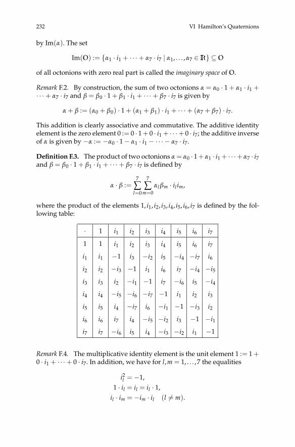
232 VI Hamilton’s Quaternions
by Im(α). The set
Im(O) := {α1 · i1 + · · ·+ α7 · i7 | α1, . . . ,α7 ∈R} ⊆O
of all octonions with zero real part is called the imaginary space of O.
Remark F.2. By construction, the sum of two octonions α = α0 · 1 + α1 · i1 +· · ·+ α7 · i7 and β = β0 · 1 + β1 · i1 + · · ·+ β7 · i7 is given by
α + β := (α0 + β0) · 1 + (α1 + β1) · i1 + · · ·+ (α7 + β7) · i7.
This addition is clearly associative and commutative. The additive identityelement is the zero element 0 := 0 · 1+ 0 · i1 + · · ·+ 0 · i7; the additive inverseof α is given by −α := −α0 · 1− α1 · i1 − · · · − α7 · i7.
Definition F.3. The product of two octonions α = α0 · 1+ α1 · i1 + · · ·+ α7 · i7and β = β0 · 1 + β1 · i1 + · · ·+ β7 · i7 is defined by
α · β :=7
∑l=0
7
∑m=0
αl βm · il im,
where the product of the elements 1, i1, i2, i3, i4, i5, i6, i7 is defined by the fol-lowing table:
· 1 i1 i2 i3 i4 i5 i6 i7
1 1 i1 i2 i3 i4 i5 i6 i7
i1 i1 −1 i3 −i2 i5 −i4 −i7 i6
i2 i2 −i3 −1 i1 i6 i7 −i4 −i5
i3 i3 i2 −i1 −1 i7 −i6 i5 −i4
i4 i4 −i5 −i6 −i7 −1 i1 i2 i3
i5 i5 i4 −i7 i6 −i1 −1 −i3 i2
i6 i6 i7 i4 −i5 −i2 i3 −1 −i1
i7 i7 −i6 i5 i4 −i3 −i2 i1 −1
Remark F.4. The multiplicative identity element is the unit element 1 := 1 +0 · i1 + · · ·+ 0 · i7. In addition, we have for l,m = 1, . . . ,7 the equalities
i2l = −1,1 · il = il = il · 1,
il · im = −im · il (l 6= m).
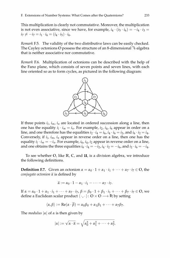
F. Extensions of Number Systems: What Comes after the Quaternions? 233
This multiplication is clearly not commutative. Moreover, the multiplicationis not even associative, since we have, for example, i4 · (i5 · i6) = −i4 · i3 =i7 6= −i7 = i1 · i6 = (i4 · i5) · i6.
Remark F.5. The validity of the two distributive laws can be easily checked.The Cayley octonions O possess the structure of an 8-dimensionalR-algebrathat is neither associative nor commutative.
Remark F.6. Multiplication of octonions can be described with the help ofthe Fano plane, which consists of seven points and seven lines, with eachline oriented so as to form cycles, as pictured in the following diagram:
i4
i1
i2
i3 i5 i6
i7
If three points il , im, in are located in ordered succession along a line, thenone has the equality il · im = in. For example, i2, i4, i6 appear in order on aline, and one therefore has the equalities i2 · i4 = i6, i4 · i6 = i2, and i6 · i2 = i4.Conversely, if il , im, in appear in reverse order on a line, then one has theequality il · im =−in. For example, i6, i4, i2 appear in reverse order on a line,and one obtains the three equalities i6 · i4 =−i2, i4 · i2 =−i6, and i2 · i6 =−i4.
To see whether O, like R, C, and H, is a division algebra, we introducethe following definitions.
Definition F.7. Given an octonion α = α0 · 1 + α1 · i1 + · · ·+ α7 · i7 ∈ O, theconjugate octonion α is defined by
α := α0 · 1− α1 · i1 − · · · − α7 · i7.
If α = α0 · 1 + α1 · i1 + · · ·+ α7 · i7, β = β0 · 1 + β1 · i1 + · · ·+ β7 · i7 ∈ O, wedefine a Euclidean scalar product 〈 · , · 〉 : O×O −→R by setting
〈α, β〉 := Re(α · β) = α0β0 + α1β1 + · · ·+ α7β7.
The modulus |α| of α is then given by
|α| :=√
α · α =√
α20 + α2
1 + · · ·+ α27.

234 VI Hamilton’s Quaternions
Remark F.8. As in Exercise 1.19, it is easily shown that for all α, β ∈ O, onehas the equalities α · β = β · α and α · α = α · α.
Remark F.9. If we identify i with i1, j with i2, and k with i3, we may theninterpret the quaternionsH in a natural way as anR-subalgebra of O. Usingthe identites i1i4 = i5, i2i4 = i6, and i3i4 = i7, we may write an octonion α =α0 · 1 + α1 · i1 + · · ·+ α7 · i7 as
α = a + b i4, (1)
with a := α0 · 1+ α1 · i1 + α2 · i2 + α3 · i3, b := α4 · 1+ α5 · i1 + α6 · i2 + α7 · i3 ∈H. For the product of two octonions α = a + b i4 and β = c + d i4, we have
α · β = (ac− db) + (da + bc)i4. (2)
Moreover, we have α = a− b i4.
Lemma F.10. The equality
α(αβ) = (αα)β (3)
holds for all α, β ∈O.
Proof. As in (1), we write α = a + b i4 and β = c + d i4. With α = a− b i4, weobtain, using (2), the equality
αβ = (ac + db) + (da− bc)i4.
Using (2) again and taking into account the associativity of multiplication inH, we obtain
α(αβ) =(a(ac + db)− (ad− cb)b
)+((da− bc)a + b(ca + bd)
)i4
=(|a|2 + |b|2)c +
((|a|2 + |b|2)d
)i4
= (αα)β,
as claimed. ut
F.2 The Octonions as a Real Division Algebra
We now proceed to show that the octonions O possess the structure of a real,normed, alternative division algebra.
Definition F.11. A nontrivial R-algebra V is said to be normed, or a com-position algebra, if V is a Euclidean vector space with scalar product 〈 · , · 〉 :V ×V −→R such that

F. Extensions of Number Systems: What Comes after the Quaternions? 235
|v · w| = |v| · |w|
for all v,w ∈ V, called the product rule.
We further define a weakened form of associativity.
Definition F.12. AnR-algebra V is said to be alternative if the equalities
v(vw) = v2w and (vw)w = vw2
hold for all v,w ∈ V.
Remark F.13. If anR-algebra V is alternative, we may compute
0 = (v(v + w))(v + w)− v(v + w)2
= (v2 + vw)(v + w)− v(v2 + vw + wv + w2)
= (vw)v− v(wv).
We therefore have the equality
(vw)v = v(wv)
for all v,w ∈ V, known as the flexible identity.
Example F.14. The R-algebras R, C, and H are normed, and since multipli-cation is associative, they are in particular alternative.
Theorem F.15. The structure (O,+, ·) is a real, normed, alternative division al-gebra of dimension 8 with unit element 1 = 1 + 0 · i1 + · · · + 0 · i7 that containsthe fields of real and complex numbers as well as the skew field of quaternions.
Proof. It is clear already that (O,+, ·) is an R-algebra of dimension 8 thatcontains R, C, and H. To prove that (O,+, ·) is a division algebra, we be-gin by showing that every nonzero octonion α possesses a multiplicativeinverse. This can be shown easily in analogy to the case of the complex num-bers or quaternions by writing
α−1 =α
|α|2 .
By Definition 1.23, we have now to show that the two equalities
α · ξ = β and η · α = β,
for α, β ∈O with α 6= 0, have unique solutions ξ,η ∈O. To this end, we shalluse the identity (3); setting ξ := α−1β = |α|−2 αβ, we then calculate

236 VI Hamilton’s Quaternions
α · ξ = |α|−2 α(αβ) = |α|−2 (αα)β = β.
Through conjugation of (3), we obtain the identity (βα)α = β(αα), whichleads to the equality
(βα)α = β(αα), (4)
valid for all α, β ∈O, since along with α, β ∈O, α, β run through all elementsof O. Setting η := βα−1 = |α|−2 βα, we thereby obtain
η · α = |α|−2(βα)α = |α|−2 β(αα) = β.
To prove that (O,+, ·) is an alternative algebra, we substitute α = 2Re(α)− αin (3) and obtain the identity
2Re(α)αβ− α(αβ) = 2Re(α)αβ− α2β,
which leads to the identity
α(αβ) = α2β
for all α, β ∈O. If we now substitute α = 2Re(α)− α in (4), we obtain analo-gously the equality
(βα)α = βα2
for all α, β ∈O. We have thereby shown that O is alternative.Finally, to show that the product rule holds, we first establish the identity
(αβ)(βα) = α((ββ)α) (5)
for all α, β ∈ O. Since this equality holds trivially for α = 0, we may assumethat α 6= 0, in which case there exists the multiplicative inverse α−1, and sinceO is a division algebra, it suffices to show that
((αβ)(βα))α = (α((ββ)α))α.
To prove this equality, we first calculate
((αβ)(βα))α = ((αβ)(αβ))α = (αβ)((αβ)α) = (αβ)((βα)α)
= (αβ)(β(αα)) = |α|2(αβ)β = |α|2α(ββ) = |α|2|β|2α,
where for the second equality, we have used (3), and for the fourth and sixthequalities, (4). But we also have
(α((ββ)α))α = (|β|2αα)α = |α|2|β|2α.

F. Extensions of Number Systems: What Comes after the Quaternions? 237
Altogether, this proves the equality (5). Finally, we calculate
|αβ|2 = (αβ)(αβ) = (αβ)(βα) = α((ββ)α) = |β|2αα = |α|2|β|2,
where for the third equality, we have used (5). This completes the proof. ut
Remark F.16. The product rule can be proved directly, but doing so is te-dious.
Remark F.17. We note that by making suitable use of the product rule, simi-larly to what was done in Exercise 1.19, one may prove the following asser-tion: If each of two natural numbers can be represented as the sum of eightsquares of natural numbers, then the product of those two numbers can alsobe represented as the sum of eight squares of natural numbers.
F.3 NormedR-Algebras
In this section, let (V, 〈 · , · 〉) be a finite-dimensional normedR-algebra withunit element 1. Conjugation on V is defined by
v := 2〈v,1〉 − v (6)
for all v ∈ V, from which one immediately deduces the relationship v = v.The validity of the product rule in its squared form
|v · w|2 = |v|2 · |w|2 (v,w ∈ V) (7)
has several immediate consequences, which we shall proceed to list.
Lemma F.18. For all t,u,v,w ∈ V, the following equalities hold:(i) 〈uv,uw〉 = |u|2〈v,w〉 and 〈vu,wu〉 = |u|2〈v,w〉.(ii) 〈tv,uw〉 = 2〈t,u〉〈v,w〉 − 〈uv, tw〉.(iii) 〈tv,w〉 = 〈v, tw〉 and 〈tv,w〉 = 〈t,wv〉.(iv) v = v and vw = w · v.
Proof. To prove (i), we consider the relationship
|v + w|2 = |v|2 + |w|2 + 2〈v,w〉 (v,w ∈ V), (8)
from which we conclude that
|uv + uw|2 = |uv|2 + |uw|2 + 2〈uv,uw〉. (9)
If, on the other hand, we replace v in (7) by u, and w by v + w, we obtain,taking into account the distributive law,
238 VI Hamilton’s Quaternions
|uv + uw|2 = |u|2 · |v + w|2 = |u|2 ·(|v|2 + |w|2 + 2〈v,w〉
), (10)
where for the last equality we have again made use of (8). Comparing (9)with (10) yields
|uv|2 + |uw|2 + 2〈uv,uw〉 = |u|2|v|2 + |u|2|w|2 + 2|u|2〈v,w〉,
which gives us the first equality on application of the product rule (7) anddivision by 2. The second equality can be proved analogously.
To prove (ii), we begin by using (i) to write(|t|2 + |u|2
)〈v,w〉 = 〈tv, tw〉+ 〈uv,uw〉,
thereby obtaining, again considering (i), the equality(|t|2 + |u|2
)〈v,w〉+ 〈tv,uw〉+ 〈uv, tw〉 = 〈(t + u)v, (t + u)w〉
= |t + u|2〈v,w〉 =(|t|2 + |u|2 + 2〈t,u〉
)〈v,w〉,
which implies the assertion.To prove (iii), we set u = 1 in (ii), which yields
〈tv,w〉 = 2〈t,1〉〈v,w〉 − 〈v, tw〉 = 〈v, (2〈t,1〉 − t)w〉 = 〈v, tw〉,
which proves the first equality. The second equality can be proved analo-gously.
To prove (iv), we have now only to prove the second equality, since thefirst has already been established. To this end, consider, using (iii), the equal-ity
〈vw,r〉 = 〈r · vw,1〉 = 〈r,vw〉 = 〈v · r,w〉 = 〈v,wr〉 = 〈w · v,r〉
for arbitrary r ∈ V, from which we conclude that vw = w · v. This completesthe proof of the lemma. ut
Definition F.19. The imaginary space of V is defined as the set
Im(V) = {v ∈ V | v /∈R \ {0} and v2 ∈R}.
Remark F.20. (i) We have Im(V) ∩ R = {0}, and v ∈ Im(V) implies λv ∈Im(V) for all λ ∈R.
(ii) Frobenius’s lemma says that Im(V) is an R-vector space and that V =R⊕ Im(V). In particular, we have the equivalence
v ∈ Im(V) ⇐⇒ 〈v,1〉 = 0,
and therefore the equality v = 2〈v,1〉 − v = −v for all v ∈ Im(V).

F. Extensions of Number Systems: What Comes after the Quaternions? 239
Theorem F.21. Every finite-dimensional normed R-algebra with unit element 1is an alternative division algebra.
Proof. First of all, by Lemma F.18 (iii) and (i), we have the respective equali-ties
〈v(vw),r〉 = 〈vw,vr〉 = |v|2〈w,r〉,〈(wv)v,r〉 = 〈wv,rv〉 = |v|2〈w,r〉,
for all r ∈ V, from which we obtain
v(vw) = |v|2w = (wv)v (11)
for all v,w ∈ V. For v ∈ V with v 6= 0, we set v−1 := v/|v|2. Multiplication of(11) by 1/|v|2 yields the equivalent equality
v−1(vw) = w = (wv)v−1, (12)
which on replacing v with v−1 and taking account of (v−1)−1 = v leads tothe equality
v(v−1w) = w = (wv−1)v.
We have thereby proved that the two equations
v · x = w and y · v = w
for v,w ∈ V with v 6= 0 possess the unique solutions x := v−1w ∈ V andy := wv−1 ∈ V, which completes the proof that V is a division algebra.
If we now substitute v = 2〈v,1〉 − v in (11), we obtain (2〈v,1〉 − v)(vw) =(v(2〈v,1〉 − v))w, from which we conclude at once that
v(vw) = v2w
for all v,w ∈ V. We prove analogously that
(vw)w = vw2
for all v,w ∈ V. Thus we have shown that V is an alternativeR-algebra. utFinally, we prove a theorem that will be of great importance in the fol-
lowing section. We recall that anR-subalgebra of V is anR-vector subspaceU ⊆ V such that for all u1,u2 ∈ U, the product u1 · u2 is also in U (see Exer-cise 1.27).
Theorem F.22. Let V be a finite-dimensional normedR-algebra with unit element1, and U (V a properR-subalgebra of V with 1 ∈U. Then there exists i = iU ∈V
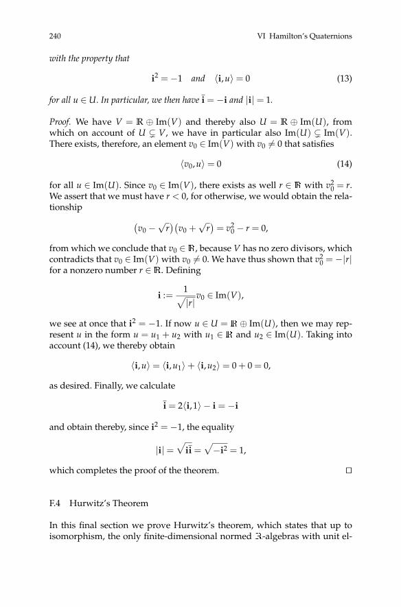
240 VI Hamilton’s Quaternions
with the property that
i2 = −1 and 〈i,u〉 = 0 (13)
for all u ∈U. In particular, we then have i = −i and |i| = 1.
Proof. We have V = R ⊕ Im(V) and thereby also U = R ⊕ Im(U), fromwhich on account of U ( V, we have in particular also Im(U) ( Im(V).There exists, therefore, an element v0 ∈ Im(V) with v0 6= 0 that satisfies
〈v0,u〉 = 0 (14)
for all u ∈ Im(U). Since v0 ∈ Im(V), there exists as well r ∈ R with v20 = r.
We assert that we must have r < 0, for otherwise, we would obtain the rela-tionship (
v0 −√
r)(
v0 +√
r)= v2
0 − r = 0,
from which we conclude that v0 ∈R, because V has no zero divisors, whichcontradicts that v0 ∈ Im(V) with v0 6= 0. We have thus shown that v2
0 =−|r|for a nonzero number r ∈R. Defining
i :=1√|r|
v0 ∈ Im(V),
we see at once that i2 = −1. If now u ∈ U = R⊕ Im(U), then we may rep-resent u in the form u = u1 + u2 with u1 ∈ R and u2 ∈ Im(U). Taking intoaccount (14), we thereby obtain
〈i,u〉 = 〈i,u1〉+ 〈i,u2〉 = 0 + 0 = 0,
as desired. Finally, we calculate
i = 2〈i,1〉 − i = −i
and obtain thereby, since i2 = −1, the equality
|i| =√
ii =√−i2 = 1,
which completes the proof of the theorem. ut
F.4 Hurwitz’s Theorem
In this final section we prove Hurwitz’s theorem, which states that up toisomorphism, the only finite-dimensional normed R-algebras with unit el-

F. Extensions of Number Systems: What Comes after the Quaternions? 241
ement 1 are the R-algebras R, C, H, and O. To prove this, we shall use theso-called Cayley–Dickson doubling process.
Proposition F.23. Let V be a finite-dimensional normed R-algebra with unit ele-ment 1. Let U ( V be a proper R-subalgebra of V with 1 ∈ U, and let i = iU ∈ Vbe an element with the property (13). Then for all a,b, c,d ∈U, the following condi-tions are satisfied:(i) 〈a + bi, c + di〉 = 〈a, c〉+ 〈b,d〉.(ii) a + bi = a− bi.(iii) bi = ib.(iv) (a + bi) · (c + di) = (ac− db) + (da + bc)i.In particular, U + Ui is anR-subalgebra of V.
Proof. To prove (i), we verify, using Lemma F.18 (iii) and (i) as well as prop-erties (13) of i the equalities
〈a,di〉 =⟨da, i
⟩= 0, 〈bi, c〉 =
⟨i,bc
⟩= 0,
and
〈bi,di〉 = |i|2〈b,d〉 = 〈b,d〉.
This gives us the first assertion.For the proof of (ii), we consider, taking into account Lemma F.18 (iii) and
(13), the equality
bi = 2〈bi,1〉 − bi = 2〈i,b〉 − bi = −bi,
from which a + bi = a + bi = a− bi follows at once.To prove (iii), we take a = 0 in (ii) and obtain, with the additional help of
Lemma F.18 (iv), the equality
−bi = bi = i · b = −ib.
This gives the third assertion.To prove (iv), we first calculate
(a + bi) · (c + di) = ac + a(di) + (bi)c + (bi)(di).
For an arbitrary v ∈ V we obtain, using Lemma F.18 (iii), the equality (iii)just proved, and Lemma F.18 (ii), the equality
〈a(di),v〉 = 〈di, av〉 = 〈id, av〉 = 0− 〈ad, iv〉 = 〈i(ad),v〉 = 〈(da)i,v〉,
where we note that 〈i, a〉 = 0. We conclude from this that a(di) = (da)i. Weverify analogously, for an arbitrary v ∈ V, using again Lemma F.18 (iii) andLemma F.18 (ii), the equality

242 VI Hamilton’s Quaternions
〈(bi)c,v〉 = 〈bi,vc〉 = 0− 〈vi,bc〉 = 〈v, (bc)i〉 = 〈(bc)i,v〉,
where we have noted that 〈i, c〉= 0. From this we conclude that (bi)c = (bc)i.Finally, we obtain analogously for an arbitrary v ∈V, using Lemma F.18 (iii),the just proved equality (iii), and Lemma F.18 (ii), the equality
〈(bi)(di),v〉 = 〈bi,v · di〉 = −〈ib,v(id)〉 = 0 + 〈vb, i(id)〉,
where we note that 〈b, id〉 = 0. A further application of Lemma F.18 (iii)and (i) now gives
〈(bi)(di),v〉 = −〈i(vb), id〉 = −|i|2〈vb,d〉 = −〈v,db〉 = 〈−db,v〉,
from which we obtain (bi)(di) = −db. Altogether, we thereby obtain
(a + bi) · (c + di) = ac + (da)i + (bc)i− db,
as asserted. This proves in particular that U + Ui is an R-subalgebra of V.ut
Remark F.24. The R-subalgebra U + Ui of V from Proposition F.23 is alsocalled the Cayley–Dickson double of U (with respect to i). The above propositionshows that whenever an R-algebra V possesses a proper R-subalgebra, itmust also contain its Cayley–Dickson double. If V is finite-dimensional, thenV itself must arise from its smallestR-subalgebra by a finite Cayley–Dicksondoubling process. In the following theorem, we shall see that the propertyof being normed allows only three Cayley–Dickson doubling processes.
Theorem F.25. Let V be a finite-dimensional normed R-algebra with unit ele-ment 1. In addition, let U ( V be a proper R-subalgebra of V with 1 ∈ U, andlet i = iU ∈ V be an element with properties (13). Then the following hold for theCayley–Dickson double U + Ui:(i) U + Ui is normed if and only if U is normed and associative.(ii) U +Ui is normed and associative if and only if U is normed, associative, and
commutative.(iii) U + Ui is normed, associative, and commutative if and only if U is normed,
associative, commutative, and invariant under conjugation.
Proof. (i) If U + Ui is normed, then U is normed. Furthermore, by Proposi-tion F.23 (iv), theR-algebra U + Ui is normed if and only if
|a + bi|2 · |c + di|2 = |(ac− db) + (da + bc)i|2
for all a,b, c,d ∈ U. By (8), (13), and Lemma F.18 (iii), this equality is equiva-lent to

F. Extensions of Number Systems: What Comes after the Quaternions? 243
(|a|2 + |b|2) · (|c|2 + |d|2) = |ac− db|2 + |da + bc|2
⇐⇒ 0 = −〈ac,db〉+ 〈da,bc〉⇐⇒ 〈d(ac),b〉 = 〈(da)c,b〉,
where we have made use of the product rule in U. This proves that U + Uiis normed if and only if d(ac) = (da)c for all a, c,d ∈ U, that is, if and only ifU is associative. Conversely, if U is normed and associative, then the aboveequivalences show that then U + Ui is normed as well.
(ii) If U + Ui is normed and associative, then U is also normed and asso-ciative. Moreover, by Proposition F.23 (iv), the equality
(ad)i = a(di) = (da)i
holds for all a,d ∈ U, which means that U is commutative. Conversely, ifU is normed, associative, and commutative, then by (i), it remains to showthat U + Ui is associative. To this end, we compute for a,b, c,d, e, f ∈ U theequalities(
(a + bi) · (c + di))· (e + f i) =
((ac− db) + (da + bc)i
)· (e + f i)
= (ac− db)e− f (da + bc) +(
f (ac− db) + (da + bc)e)i
= (ac)e− (db)e− f (da)− f (bc) +(
f (ac)− f (db) + (da)e + (bc)e)i
and
(a + bi) ·((c + di) · (e + f i)
)= (a + bi) ·
((ce− f d) + ( f c + de)i
)= a(ce− f d)− ( f c + de)b +
(( f c + de)a + b(ce− f d)
)i
= a(ce)− a( f d)− (c f )b− (ed)b +(( f c)a + (de)a + b(e c)− b(d f )
)i.
Since U is associative and commutative, these two expressions agree. Thisproves that U + Ui is associative.
(iii) If U + Ui is normed, associative, and commutative, then U is alsonormed, associative, and commutative. Moreover, we have then by Propo-sition F.23 (iii) the equality
ia = ai = ia
for all a ∈ U; that is, we have a = a for all a ∈ U. Therefore, U is invariantunder conjugation. Conversely, if U is normed, associative, commutative,and invariant under conjugation, then by (ii), it remains to show that U +Uiis commutative. To prove this, we calculate for a,b, c,d ∈U the equalities
(a + bi) · (c + di) = (ac− db) + (da + bc)i,
(c + di) · (a + bi) = (ca− bd) + (bc + da)i.

244 VI Hamilton’s Quaternions
Since U is associative, commutative, and invariant under conjugation, thetwo expressions agree. This proves that U + Ui is commutative. ut
Example F.26. Starting with the 1-dimensional associative, commutative,and conjugation-invariant R-algebra R, we obtain by the Cayley–Dicksondoubling process the 2-dimensional associative and commutativeR-algebraC ∼= R + Ri. If in a further step we apply the Cayley–Dickson doublingprocess to the R-algebra of complex numbers C, we will arrive at the 4-dimensional associativeR-algebraH∼=C+Cj. By Remark F.9, we obtain fi-nally in a third Cayley–Dickson step applied to theR-algebra of quaternionsthe 8-dimensional algebra O ∼=H+Hi4 of octonions. This example demon-strates quite clearly the successive loss of conjugation-invariance, commuta-tivity, and associativity through repeated application of the Cayley–Dicksondoubling process.
Theorem F.27 (Hurwitz’s theorem). The R-algebras R, C,H, and O are (up toisomorphism) the only finite-dimensional normed R-algebras with unit element 1.
Proof. Let V be a finite-dimensional normed R-algebra with unit element 1.We shall show that V is isomorphic to R, C,H, or O.
If V is 1-dimensional, then V is isomorphic to R. Otherwise, V has aproper R-subalgebra U1 ( V that is isomorphic to R. We have 1 ∈ U1,and by Theorem F.22, there exists i = iU1 ∈ V satisfying properties (13). ByTheorem F.25, the Cayley–Dickson double U1 + U1iU1 is a normed, asso-ciative, and commutative R-subalgebra of V, since U1
∼= R is normed, as-sociative, commutative, and invariant under conjugation. If we now haveV = U1 + U1iU1 , then V is isomorphic toR+RiU1
∼=C.Otherwise, V possesses a properR-subalgebra U2 (V that is isomorphic
to C. We again have 1 ∈ U2, and by Theorem F.22, there exists i = iU2 ∈V satisfying properties (13). By Theorem F.25, the Cayley–Dickson doubleU2 + U2iU2 is a normed and associative R-subalgebra of V, since U2 ∼= Cis normed, associative, and commutative. If we now have V = U2 + U2iU2 ,then V is isomorphic to C+CiU2
∼=H.Otherwise, V possesses a proper R-subalgebra U3 ( V isomorphic to H.
We again have 1 ∈U3, and by Theorem F.22, there exists i = iU3 ∈ V satisfy-ing properties (13). By Theorem F.25, the Cayley–Dickson double U3 +U3iU3is a normed R-subalgebra of V, since U3 ∼=H is normed and associative. Ifwe now have V = U3 + U3iU3 , then V is isomorphic toH+HiU3
∼= O.If now V were to contain a properR-subalgebra U4 (V isomorphic to O,
then we would again have 1 ∈ U4, and by Theorem F.22, there would existi = iU4 ∈ V satisfying properties (13). By Theorem F.25, the Cayley–Dicksondouble U4 + U4iU4 would not, however, be a normed R-subalgebra of V,since U4
∼= O is not associative. This contradicts the fact that V is normed.This case can therefore not occur, and the theorem is proved. ut

F. Extensions of Number Systems: What Comes after the Quaternions? 245
Remark F.28. The statement of Hurwitz’s theorem holds more generally forfinite-dimensional real division algebras that are not necessarily normed.In this context, Heinz Hopf showed in [5], already in 1940, that the dimen-sion of such a division algebra must be a power of 2. In 1958, Michel Ker-vaire and John Milnor proved in [7], independently of each other, that everyfinite-dimensional real division algebra has dimension 1, 2, 4, or 8. It thenfollows from this more general assumption that every such division algebrais isomorphic to R, C, H, or O. The proof of the deep theorem of Kervaire–Milnor uses methods of algebraic topology (see Chapter 10, contributed byFriedrich Hirzebruch, in [4]). As of today, there is no known purely algebraicproof.
If one applies the Cayley–Dickson doubling process again to the skewfield of octonions, one obtains the 16-dimensional R-algebra S of sedenions,which is neither commutative nor alternative; it is also not associative, and ithas zero divisors, and is therefore, as we know by now, no longer a divisionalgebra.
Remark F.29. We end this section with the observation that there is an al-ternative way to construct higher-dimensional R-algebras containing R, C,and H beginning with the real numbers and passing to the complex num-bers and the quaternions. To do so, we begin with an n-dimensional Eu-clideanR-vector space (V, 〈 · , · 〉); we note that we could as well begin moregenerally with a K-vector space, over an arbitrary field K, and an arbitraryscalar product. We then form the tensor algebra T(V) and consider its ideal
I(V) =⟨v⊗ w + w⊗ v + 2 · 〈v,w〉
∣∣v,w ∈ V⟩.
We then define the so-called Clifford algebra
C(V, 〈 · , · 〉) := T(V)/I(V),
in which we denote the product by · as usual. The Clifford algebra is by con-struction an associativeR-algebra of dimension 2n. Namely if {e1, . . . , en} isan ordered orthonormal basis of V, then C(V, 〈 · , · 〉) has the basis
{1; e1, . . . , en; e1 · e2, e1 · e3, . . . , en−1 · en; . . . ; e1 · · · en},
from which, on account of(n0
)+
(n1
)+
(n2
)+ · · ·+
(nn
)= 2n,
we can easily read off the dimension of C(V, 〈 · , · 〉).If n = 0, we obtain C(V, 〈 · , · 〉) ∼=R. For n = 1, we have C(V, 〈 · , · 〉) ∼=C.
Namely, if V is generated by i := e1, then C(V, 〈 · , · 〉) is generated by 1 and iwith i2 =−1. For n = 2, we obtain C(V, 〈 · , · 〉)∼=H; namely, if V is generated

246 VI Hamilton’s Quaternions
by i := e1 and j := e2, then C(V, 〈 · , · 〉) will be generated by 1, i, j, and k :=e1 · e2, where i2 = j2 = k2 = −1 and i · j = k = −j · i. For n = 3, one obtains,however, C(V, 〈 · , · 〉) ∼=H×H; associativity is preserved, but one loses theproperty of being a division algebra, since now C(V, 〈 · , · 〉) is no longer freeof zero divisors.
The Clifford algebra C(V, 〈 · , · 〉) associated with an n-dimensional Eu-clidean vector space (V, 〈 · , · 〉) makes it possible to generalize the relation-ship described in Section 3 of this chapter between the special orthogonalgroup SO3(R) and the quaternions S3 of modulus 1 with the help of thespinor representation of the special orthogonal group SOn(R) in the group ofinvertible elements of C(V, 〈 · , · 〉).
References
[1] J. C. Baez: The octonions. Bull. Amer. Math. Soc. (N.S.) 39 (2002), 145–205.[2] J. C. Baez: Errata for: “The octonions” [Bull. Amer. Math. Soc. (N.S.) 39 (2002),
145–205]. Bull. Amer. Math. Soc. (N.S.) 42 (2005), 213.[3] J. H. Conway and D. A. Smith: On quaternions and octonions: their geometry, arith-
metic, and symmetry. A K Peters, Natick, MA, 2003.[4] H. Ebbinghaus et al.: Numbers. Translated from the 2nd German 1988 edition
by H. L. S. Orde. Springer, Berlin Heidelberg New York, 1991.[5] H. Hopf: Ein topologischer Beitrag zur reellen Algebra. Comm. Math. Helvetici 13
(1940/41), 427–440.[6] A. Hurwitz: Über die Komposition der quadratischen Formen. Math. Ann. 88
(1922), 1–25.[7] J. Milnor: Some consequences of a theorem of Bott. Ann. of Math. (2) 68 (1958),
444–449.[8] B. L. van der Waerden: A history of algebra. From al-Khwarizmi to Emmy Noether.
Springer, Berlin Heidelberg New York, 1985.

Solutions to Exercises
In this chapter we present solutions to some exercises along with hints forhelping to solve others.
Solutions to Exercises in Chapter I
Exercise 1.8. We prove first the validity of the associative law of addition,that is, the equality
n + (m + p) = (n + m) + p (1)
for all n, m, p ∈N. We do this by induction on p. For p = 0, the assertion isclear. Suppose, then, that assertion (1) holds for an arbitrary but fixed p ∈Nand for all n, m ∈N. Then from the definition of addition and the inductionhypothesis, we have the equality
(n + m) + p∗ = ((n + m) + p)∗ = (n + (m + p))∗
= n + (m + p)∗ = n + (m + p∗),
as desired. This proves the associativity of addition. The first distributivelaw, that is, the equality
(n + m) · p = n · p + m · p (2)
for all n, m, p ∈N, can be proved using the associativity and commutativityof addition along with induction on p. For p = 0, the assertion is clear. Sup-pose now that (2) holds for an arbitrary but fixed p ∈N and for all n, m ∈N.Then we have
(n + m) · p∗ = (n + m) · p + (n + m) = (n · p + m · p) + (n + m)
= (n · p + n) + (m · p + m) = n · p∗ + m · p∗,
as desired. This proves the asserted distributivity. Using the first distributivelaw, one can then prove the commutativity of multiplication by induction.This then also yields the validity of the second distributive law. Finally, onecan prove the associativity of multiplication by induction.
Exercise 1.10. Let m, n ∈ N. If m = 0 or n = 0, then one immediately hasthe equality m · n = 0 by Definition 1.5 (2) and the commutativity of mul-
© Springer International Publishing AG 2017
Springer Undergraduate Mathematics Series, https://doi.org/10.1007/978-3-319-69429-0J. Kramer and A.-M. von Pippich, From Natural Numbers to Quaternions,
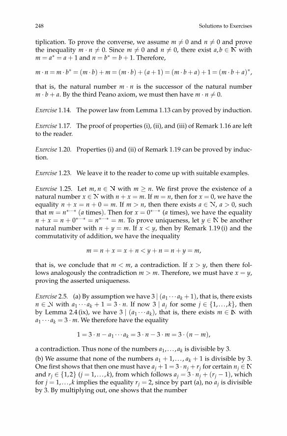
248 Solutions to Exercises
tiplication. To prove the converse, we assume m 6= 0 and n 6= 0 and provethe inequality m · n 6= 0. Since m 6= 0 and n 6= 0, there exist a,b ∈ N withm = a∗ = a + 1 and n = b∗ = b + 1. Therefore,
m · n = m · b∗ = (m · b) +m = (m · b) + (a+ 1) = (m · b+ a) + 1 = (m · b+ a)∗,
that is, the natural number m · n is the successor of the natural numberm · b + a. By the third Peano axiom, we must then have m · n 6= 0.
Exercise 1.14. The power law from Lemma 1.13 can by proved by induction.
Exercise 1.17. The proof of properties (i), (ii), and (iii) of Remark 1.16 are leftto the reader.
Exercise 1.20. Properties (i) and (ii) of Remark 1.19 can be proved by induc-tion.
Exercise 1.23. We leave it to the reader to come up with suitable examples.
Exercise 1.25. Let m, n ∈ N with m ≥ n. We first prove the existence of anatural number x ∈N with n + x = m. If m = n, then for x = 0, we have theequality n + x = n + 0 = m. If m > n, then there exists a ∈ N, a > 0, suchthat m = n∗···∗ (a times). Then for x = 0∗···∗ (a times), we have the equalityn + x = n + 0∗···∗ = n∗···∗ = m. To prove uniqueness, let y ∈ N be anothernatural number with n + y = m. If x < y, then by Remark 1.19 (i) and thecommutativity of addition, we have the inequality
m = n + x = x + n < y + n = n + y = m,
that is, we conclude that m < m, a contradiction. If x > y, then there fol-lows analogously the contradiction m > m. Therefore, we must have x = y,proving the asserted uniqueness.
Exercise 2.5. (a) By assumption we have 3 | (a1 · · · ak + 1), that is, there existsn ∈ N with a1 · · · ak + 1 = 3 · n. If now 3 | aj for some j ∈ {1, . . . ,k}, thenby Lemma 2.4 (ix), we have 3 | (a1 · · · ak), that is, there exists m ∈ N witha1 · · · ak = 3 ·m. We therefore have the equality
1 = 3 · n− a1 · · · ak = 3 · n− 3 ·m = 3 · (n−m),
a contradiction. Thus none of the numbers a1, . . . , ak is divisible by 3.(b) We assume that none of the numbers a1 + 1, . . . , ak + 1 is divisible by 3.One first shows that then one must have aj + 1 = 3 · nj + rj for certain nj ∈Nand rj ∈ {1,2} (j = 1, . . . ,k), from which follows aj = 3 · nj + (rj − 1), whichfor j = 1, . . . ,k implies the equality rj = 2, since by part (a), no aj is divisibleby 3. By multiplying out, one shows that the number

Solutions to Exercises in Chapter I 249
a1 · · · ak − 1 =k
∏j=1
(3 · nj + 1)− 1
is divisible by 3. But this contradicts the assumption that a1 · · · ak + 1 is di-visible by 3. Therefore, at least one of the numbers a1 + 1, . . . , ak + 1 must bedivisible by 3.
Exercise 2.12. To make the proceedings clear, we calculate first, with a1 = 2and an+1 = (an − 1) · an + 1 for n ∈ N, n ≥ 1, the numbers a2 = 3, a3 = 7,a4 = 43, a5 = 1807, a6 = (1807− 1) · 1806+ 1 = 3263443. WithMn = {p∈P |p | an}, we obtain the first six sets,
M1 = {2}, M2 = {3}, M3 = {7}, M4 = {43},M5 = {13, 139}, M6 = {3263443}.
We claim that we have the equality an = 5 · bn + rn with bn ∈N and rn ∈ {2,3}(n ∈N, n≥ 1). This can be proved by induction on n. If n = 1, the assertion isclear. We now assume that the assertion holds for arbitrary but fixed n ∈N,n ≥ 1. Then we have
an+1 = (an − 1) · an + 1 = (5 · bn + rn − 1) · (5 · bn + rn) + 1
= 5 · (5b2n + 2bnrn − bn) + r2
n − rn + 1.
If rn = 2, then r2n− rn + 1 = 3; if rn = 3, then r2
n− rn + 1 = 5+ 2. Therefore, inboth cases, an+1 is of the form 5 · bn+1 + rn+1 with bn+1 ∈N and rn+1 ∈ {2,3},as desired. We have thus shown that 5 - an, that is, 5 /∈ Mn, for all n ∈ N,n ≥ 1.
Exercise 2.13. Let us assume, contrary to the assertion, that there are onlyfinitely many prime numbers p1, . . . , pn in 2 + 3 ·N. We then consider thenatural number
a := 3 · p1 · · · pn − 1.
We have that a > 1, and by Lemma 2.9, a has a prime divisor p. Since 3 - a,it follows that p 6= 3. We now show that p ∈ 2 + 3 ·N; that is, we must showthat 3 | (p + 1). If p = a, we are done. If p < a, then there exists q ∈N, q > 1,with a = p · q. Since 3 | (p · q + 1), it follows by Exercise 2.5 (b) that 3 | (p + 1)or 3 | (q + 1). In the first case, we are done. In the second case, we repeat theprocess for a prime divisor of q. Finally, after finitely many steps, we obtaina prime divisor p of a with p ∈ 2 + 3 ·N. We now proceed as in Euclid’sproof, for on the assumption that there are only finitely many prime num-bers in the set 2+ 3 ·N, we must have p∈ {p1, . . . , pn}. In particular, we havep | (p1 · · · pn). However, since we have the divisibility relation p | a, we musthave p | 1 from the divisibility rules, which is a contradiction.
Exercise 2.15. We prove the contrapositive of the asserted implication.

250 Solutions to Exercises
(i) Suppose that n is not a prime. Then there exist natural numbers a,b ∈Nwith n = a · b and 1 < a,b < n. We thus obtain
2n − 1 = 2a·b − 1 = (2a − 1) · (2a·(b−1) + 2a·(b−2) + · · ·+ 2a + 1).
Since 1 < 2a − 1 < 2n − 1, it follows that 2a − 1 is a nontrivial divisor of2n − 1, which proves that 2n − 1 is not prime.(ii) Let n ∈ N, n > 0, with n not a power of 2. Then n > 2, and there existnatural numbers a,b ∈ N, b odd, with n = a · b and 1 ≤ a < n, 1 < b ≤ n.Since b is odd, we obtain
2n + 1 = 2a·b + 1 = (2a + 1) · (2a·(b−1) ∓ · · · − 2a + 1).
Since 1 < 2a + 1 < 2n + 1, it follows that 2a + 1 is a nontrivial divisor of2n + 1, which proves that 2n + 1 is not prime.
Exercise 2.18. Let {a1, . . . , an} and {b1, . . . , bm} denote the sets of all divisorsof a and all divisors of b. Since a and b are relatively prime, the set of alldivisors of a · b is equal to {aj · bk | j = 1, . . . , n; k = 1, . . . , m}. It follows that
S(a) · S(b) = (a1 + · · ·+ an) · (b1 + · · ·+ bm) =n
∑j=1
m
∑k=1
aj · bk = S(a · b).
This completes the proof of the assertion.
Exercise 2.19. The assertion can be proved by induction on m.
Exercise 2.20. (a) We have the equalities
S(220)− 220 = 1 + 2 + 4 + 5 + 10 + 11 + 20 + 22 + 44 + 55 + 110 = 284,S(284)− 284 = 1 + 2 + 3 + 71 + 142 = 220.
Therefore, we have S(220) = 220 + 284 = S(284), which proves that thenumbers 220 and 284 are amicable.(b) We must show that S(a) = a + b = S(b). Since x,y,z are distinct oddprimes, it follows that
S(a) = S(2n · x · y) = S(2n) · S(x) · S(y) = (2n+1 − 1)(x + 1)(y + 1),
S(b) = S(2n) · S(z) = (2n+1 − 1)(z + 1),
where we have used the well-known equality S(2n) = 2n+1 − 1. A directcalculation shows that x · y = 9 · 22n−1 − 9 · 2n−1 + 1, and therefore, x · y +x + y = z. This implies S(a) = (2n+1− 1)(z + 1) = S(b). Finally, we calculate
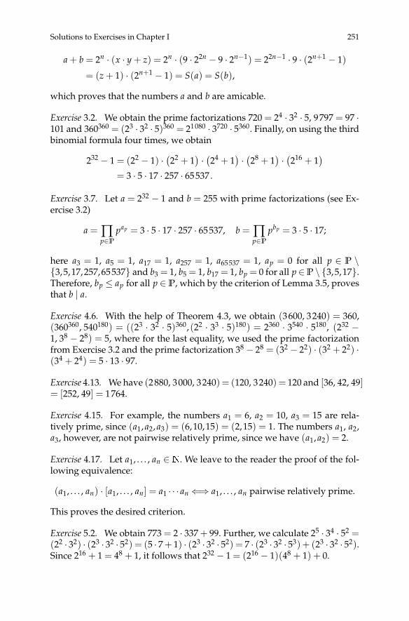
Solutions to Exercises in Chapter I 251
a + b = 2n · (x · y + z) = 2n · (9 · 22n − 9 · 2n−1) = 22n−1 · 9 · (2n+1 − 1)
= (z + 1) · (2n+1 − 1) = S(a) = S(b),
which proves that the numbers a and b are amicable.
Exercise 3.2. We obtain the prime factorizations 720 = 24 · 32 · 5, 9797 = 97 ·101 and 360360 = (23 · 32 · 5)360 = 21080 · 3720 · 5360. Finally, on using the thirdbinomial formula four times, we obtain
232 − 1 = (22 − 1) ·(22 + 1
)·(24 + 1
)·(28 + 1
)·(216 + 1
)= 3 · 5 · 17 · 257 · 65537.
Exercise 3.7. Let a = 232 − 1 and b = 255 with prime factorizations (see Ex-ercise 3.2)
a = ∏p∈P
pap = 3 · 5 · 17 · 257 · 65537, b = ∏p∈P
pbp = 3 · 5 · 17;
here a3 = 1, a5 = 1, a17 = 1, a257 = 1, a65537 = 1, ap = 0 for all p ∈ P \{3,5,17,257,65537} and b3 = 1, b5 = 1, b17 = 1, bp = 0 for all p∈P \ {3,5,17}.Therefore, bp ≤ ap for all p ∈ P, which by the criterion of Lemma 3.5, provesthat b | a.
Exercise 4.6. With the help of Theorem 4.3, we obtain (3600, 3240) = 360,(360360, 540180) = ((23 · 32 · 5)360, (22 · 33 · 5)180) = 2360 · 3540 · 5180, (232 −1, 38 − 28) = 5, where for the last equality, we used the prime factorizationfrom Exercise 3.2 and the prime factorization 38 − 28 = (32 − 22) · (32 + 22) ·(34 + 24) = 5 · 13 · 97.
Exercise 4.13. We have (2880, 3000, 3240) = (120, 3240) = 120 and [36, 42, 49]= [252, 49] = 1764.
Exercise 4.15. For example, the numbers a1 = 6, a2 = 10, a3 = 15 are rela-tively prime, since (a1, a2, a3) = (6,10,15) = (2,15) = 1. The numbers a1, a2,a3, however, are not pairwise relatively prime, since we have (a1, a2) = 2.
Exercise 4.17. Let a1, . . . , an ∈N. We leave to the reader the proof of the fol-lowing equivalence:
(a1, . . . , an) · [a1, . . . , an] = a1 · · · an⇐⇒ a1, . . . , an pairwise relatively prime.
This proves the desired criterion.
Exercise 5.2. We obtain 773 = 2 · 337 + 99. Further, we calculate 25 · 34 · 52 =(22 · 32) · (23 · 32 · 52) = (5 · 7+ 1) · (23 · 32 · 52) = 7 · (23 · 32 · 53)+ (23 · 32 · 52).Since 216 + 1 = 48 + 1, it follows that 232 − 1 = (216 − 1)(48 + 1) + 0.

252 Solutions to Exercises
Exercise 5.4. This process can be carried out for arbitrary natural numbersg > 1. One obtains the unique representation
n = q` · g` + q`−1 · g`−1 + · · ·+ q1 · g1 + q0 · g0
with natural numbers 0≤ qj ≤ g− 1 (j = 0, . . . , `) and q` 6= 0, called the g-adicrepresentation of the natural number n.
Solutions to Exercises in Chapter II
Exercise 1.3. For a, b, c ∈ Rn, one has the equalities
(a⊕ b)⊕ c =Rn(a + b)⊕ c =Rn(Rn(a + b) + c),a⊕ (b⊕ c) = a⊕Rn(b + c) =Rn(a +Rn(b + c)).
Division with remainder of a + b and b + c by n yields the uniquely deter-mined numbers q1, q2 ∈N such that
a + b = q1 · n +Rn(a + b) and b + c = q2 · n +Rn(b + c),
whence follows
Rn(Rn(a + b) + c) =Rn(a + b + c− q1 · n) =Rn(a + b + c)=Rn(a + b + c− q2 · n) =Rn(a +Rn(b + c)).
We have thereby shown that the operation ⊕ is associative. Analogously,one can prove that the operation � is associative.
Exercise 1.4. (a) The set 2 ·N = {2 · n | n ∈N} of even natural numbers is anonempty subset ofN. If 2 ·m, 2 · n ∈ 2 ·N, then
2 ·m + 2 · n = 2 · (m + n) ∈ 2 ·N, (2 ·m) · (2 · n) = 2 · (m · 2 · n) ∈ 2 ·N.
Thus both + and · are operations on 2 ·N. Since the operations + onN and· onN are associative, it follows that in particular, the operations + on 2 ·Nand · on 2 ·N are associative. Therefore, both (2 ·N, +) and (2 ·N, ·) aresemigroups.
The set 2 · N + 1 = {2 · n + 1 | n ∈ N} of odd natural numbers is anonempty subset ofN. If 2 ·m + 1 and 2 · n + 1 are in 2 ·N+ 1, then
(2 ·m + 1) + (2 · n + 1) = 2 · (m + n + 1) ∈ 2 ·N,(2 ·m + 1) · (2 · n + 1) = 2 · (m · 2 · n + m + n) + 1 ∈ 2 ·N+ 1.

Solutions to Exercises in Chapter II 253
Therefore, while · is an operation on 2 ·N+ 1, we see that + is not an opera-tion on 2 ·N+ 1. Therefore, (2 ·N+ 1, +) is not a semigroup. The operation ·on N is associative, and so in particular, the operation · on 2 ·N+ 1 is asso-ciative. Therefore, (2 ·N+ 1, ·) is a semigroup.(b) Let k ∈ N, k > 1. The set k ·N = {k · n | n ∈ N} is a nonempty subset ofN. One shows, as in (a), that both (k ·N, +) and (k ·N, ·) are semigroups.
Exercise 1.5. Because of the inequality
(2 ◦ 3) ◦ 2 = (23) ◦ 2 = (23)2 = 23·2 = 26 6= 29 = 2 ◦ (32) = 2 ◦ (3 ◦ 2),
the operation ◦ on N is not associative, and therefore (N, ◦) is not a semi-group.
Exercise 1.8. If A1 = {a1} is a one-element set, then
map(A1) = {id},
where the mapping id : A1 −→ A1 is given by the assignment a1 7→ a1. Thesemigroup (map(A1),◦) is abelian. If A2 = {a1, a2, . . .} is an arbitrary setthat contains at least two elements a1 6= a2, then
map(A2) = {id, f , g, . . .},
where the mapping id : A2 −→ A2 is given by aj 7→ aj (aj ∈ A2), the mappingf : A2−→ A2 by a1 7→ a2, aj 7→ aj (aj ∈ A2 \ {a1}), and the mapping g : A2−→A2 by a2 7→ a1, aj 7→ aj (aj ∈ A2 \ {a2}). But then we have
( f ◦ g)(a1) = f (g(a1)) = f (a1) = a2 6= a1 = g(a2) = g( f (a1)) = (g ◦ f )(a1),
whence (map(A2), ◦) is a nonabelian semigroup.
Exercise 1.12. Let e` be a left identity element and er a right identity elementof H. Then
e` = e` ◦ er = er,
where the first equality follows from the fact that er is a right identity el-ement of H, and the second from the fact that e` is a left identity elementof H.
Exercise 1.14. (a) By Exercise 1.4, (2 ·N,+) and (2 ·N, ·) are semigroups.It remains to show that there exists an additive identity element in 2 ·N.By the definition of addition, 0 is this element. Since 1 6∈ 2 ·N, there is nomultiplicative identity element, so that (2 ·N, ·) is only a semigroup.(b) We leave it to the reader to find other examples of semigroups that arenot monoids.

254 Solutions to Exercises
Exercise 2.3. (a) Suppose that g′ and g′′ are two inverse elements to an ele-ment g ∈ G. Then
g′ = g′ ◦ e = g′ ◦ (g ◦ g′′) = (g′ ◦ g) ◦ g′′ = e ◦ g′′ = g′′ ,
where the second equality follows from the fact that g′′ is in particular aright inverse to g, and the fourth equality follows from the fact that g′ is inparticular a left inverse to g.(b) Let g′` be a left inverse and g′r a right inverse to an element g ∈ G. Then itfollows that
g′` = g′` ◦ e = g′` ◦ (g ◦ g′r) = (g′` ◦ g) ◦ g′r = e ◦ g′r = g′r,
analogously to part (a).
Exercise 2.6. (a) Let g−1 ∈ G be the inverse element to g ∈ G. Then
g ◦ g−1 = e = g−1 ◦ g.
Thus g is the inverse element to g−1, that is, (g−1)−1 = g.(b) Let g−1 ∈ G be the inverse element to g ∈ G and h−1 ∈ G the inverseelement to h ∈ G. Then
(h−1 ◦ g−1) ◦ (g ◦ h) = h−1 ◦ (g−1 ◦ g) ◦ h = h−1 ◦ e ◦ h = h−1 ◦ h = e,
(g ◦ h) ◦ (h−1 ◦ g−1) = g ◦ (h ◦ h−1) ◦ g−1 = g ◦ e ◦ g−1 = g ◦ g−1 = e.
Thus h−1 ◦ g−1 is the inverse element to g ◦ h, that is, (g ◦ h)−1 = h−1 ◦ g−1.The calculational rules (c) and (d) follow directly from the definition.
Exercise 2.9. We compare only the groups that have the same numbers of el-ements. The Cayley tables of the groups (R4,⊕), (R5 \ {0},�), and (D4, ◦)have, reading from left to right, the following form:
⊕ 0 1 2 30 0 1 2 31 1 2 3 02 2 3 0 13 3 0 1 2
� 1 2 3 41 1 2 3 42 2 4 1 33 3 1 4 24 4 3 2 1
◦ d0 d1 s0 s1
d0 d0 d1 s0 s1d1 d1 d0 s1 s0s0 s0 s1 d0 d1s1 s1 s0 d1 d0
One may conclude from the Cayley tables that all three groups under con-sideration are abelian. We now determine the smallest nonzero natural num-ber n such that gn = e for g 6= e. In the group (R4,⊕), we have e = 0 and
12 = 2, 13 = 3, 14 = 0; 22 = 0; 32 = 2, 33 = 1, 34 = 0.
In the group (R5 \ {0},�), we have e = 1 and

Solutions to Exercises in Chapter II 255
22 = 4, 23 = 3, 24 = 1; 32 = 4, 33 = 2, 34 = 1; 42 = 1.
Thus in each group there are two elements with n = 4 and one element withn = 2. In the group (D4, ◦), however, d2
1 = s20 = s2
1 = e with e = d0, that is,there is no element with n = 4.The Cayley tables for (R6,⊕) and (D6, ◦), reading from left to right, havethe following form:
⊕ 0 1 2 3 4 50 0 1 2 3 4 51 1 2 3 4 5 02 2 3 4 5 0 13 3 4 5 0 1 24 4 5 0 1 2 35 5 0 1 2 3 4
◦ d0 d1 d2 s0 s1 s2
d0 d0 d1 d2 s0 s1 s2d1 d1 d2 d0 s2 s0 s1d2 d2 d0 d1 s1 s2 s0s0 s0 s1 s2 d0 d1 d2s1 s1 s2 s0 d2 d0 d1s2 s2 s0 s1 d1 d2 d0
From these tables, one can see that the group (R6,⊕) is abelian. The group(D6, ◦) is nonabelian, since s0 ◦ s1 = d2 6= d1 = s1 ◦ s0. We again determinethe smallest nonzero natural number n such that gn = e for g 6= e. In (R6,⊕),we have e = 0 and
12 = 2, 13 = 3, 14 = 4, 15 = 5, 16 = 0; 22 = 4, 23 = 0; 32 = 0;
42 = 2, 43 = 0; 52 = 4, 53 = 3, 54 = 2, 55 = 1, 56 = 0.
There exist, therefore, in (R6,⊕) two elements with n = 6, two elementswith n = 3, and one element with n = 2. In (D6, ◦), we have e = d0 and
d21 = d2, d3
1 = d0; d22 = d1, d3
2 = d0; s20 = d0, s2
1 = d0, s22 = d0.
There exist, therefore, in (D6, ◦) no element with n = 6, two elements withn = 3, and three elements with n = 2.
Exercise 2.10. (a) One shows using the Cayley table
� 1 21 1 22 2 1
for (R3 \ {0},�) and the Cayley table from Exercise 2.9 for (R5 \ {0},�)that (R3 \ {0},�) and (R5 \ {0},�) are groups.(b) We leave to the reader the task of verifying the assertions of Exam-ple 2.8 (iii) regarding the dihedral group (D2n, ◦).(c) Let n ≥ 3. We consider the elements
π1 =
(1 2 3 · · · n2 1 3 · · · n
), π2 =
(1 2 3 · · · n3 1 2 · · · n
)

256 Solutions to Exercises
of Sn, where for n > 3, each of the elements 4, . . . ,n is mapped to itself. Then
π1 ◦ π2 =
(1 2 3 · · · n3 2 1 · · · n
)6=(
1 2 3 · · · n1 3 2 · · · n
)= π2 ◦ π1,
where for n > 3, each of the elements 4, . . . ,n is mapped to itself. This provesthat (Sn, ◦) for n ≥ 3 is nonabelian.
Exercise 2.13. This is proved by induction on n.
Exercise 2.19. We have S3 = {π1, π2, π3, π4, π5, π6} with
π1 =
(1 2 31 2 3
), π2 =
(1 2 32 3 1
), π3 =
(1 2 33 1 2
),
π4 =
(1 2 31 3 2
), π5 =
(1 2 33 2 1
), π6 =
(1 2 32 1 3
).
We calculate ord(π1) = 1, ord(π2) = ord(π3) = 3, and ord(π4) = ord(π5) =ord(π6) = 2.
Exercise 2.23. Since dk1 = dk (k = 0, . . . ,n − 1) and dn
1 = d0, we have 〈d1〉 ={d0, . . . , dn−1}. Using the subgroup criterion, one can show that the nonemptysubset 〈g〉= {. . . , (g−1)2, g−1, g0 = e, g1 = g, g2, . . .} ⊆ G is a subgroup of Gfor every group G. In particular, 〈d1〉 = {d0, . . . , dn−1} is a subgroup of D2n.
Exercise 2.26. We have S3 = {π1, π2, π3, π4, π5, π6} with πj (j = 1, . . . ,n) asin Exercise 2.19. We have the cyclic subgroups
〈π1〉 = {π1}, 〈π2〉 = {π1,π2,π3} = 〈π3〉 ,〈π4〉 = {π1,π4}, 〈π5〉 = {π1,π5}, 〈π6〉 = {π1,π6} ,
and the subgroup S3 itself, which is not cyclic. One can see that S3 has noother subgroups.
Exercise 3.3. We have S3 = {π1, π2, π3, π4, π5, π6} with πj (j = 1, . . . ,n) asin Exercise 2.19 and D6 = {d0, d1, d2, d0 ◦ s0, d1 ◦ s0, d2 ◦ s0}, where s0 is re-flection in the median of the side joining vertices 1 and 2. By the definitionof the group homomorphism f : D6 −→ S3, we have
f (d0) = π1, f (d1) = π3, f (d2) = π2,f (d0 ◦ s0) = π6, f (d1 ◦ s0) = π5, f (d2 ◦ s0) = π4,
which proves that f is bijective and therefore in fact a group isomorphism.
Exercise 3.5. Let dj1 ◦ sk10 and dj2 ◦ sk2
0 with j1, j2 ∈ {0, . . . , n− 1} and k1, k2 ∈{0, 1} be two elements of D2n. Since dj ◦ s0 = s0 ◦ d−1
j , we have

Solutions to Exercises in Chapter II 257
(dj1 ◦ sk10 ) ◦ (dj2 ◦ sk2
0 ) =
dj1 ◦ dj2 , if k1 = 0, k2 = 0;dj1 ◦ dj2 ◦ s0, if k1 = 0, k2 = 1;dj1 ◦ d−1
j2, if k1 = 1, k2 = 1;
dj1 ◦ d−1j2◦ s0, if k1 = 1,k2 = 0.
It follows that
sgn((
dj1 ◦ sk10)◦(dj2 ◦ sk2
0))
= k1 ⊕ k2 = sgn(dj1 ◦ sk1
0)⊕ sgn
(dj2 ◦ sk2
0).
Therefore, sgn is a group homomorphism, and we have im(sgn) = R2 andker(sgn) = {dj | j = 0, . . . , n− 1}.
Exercise 3.7. By Lemma 3.6, we have f injective⇐⇒ ker( f ) = {eG}. It there-fore suffices to prove, under the assumption |G| < ∞, the equivalence f in-jective⇐⇒ f surjective. We have
f injective ⇐⇒ g 6= h for g, h ∈ G implies f (g) 6= f (h)
⇐⇒|G|<∞
| f (G)| = |G|
⇐⇒ for every g ∈ G there exists h ∈ G with f (h) = g⇐⇒ f surjective.
This proves the assertion.
Exercise 3.8. If g ∈ G and ord(g) = n, then e = f (e) = f (gn) = f (g)n, whichimplies ord
(f (g)
)≤ n = ord(g).
Exercise 3.9. Suppose that f : D24 −→ S4 is a group isomorphism. Then foreach g ∈ D24, we must have the equality
ord(g) = ord( f (g)).
Since ord(d2) = 12, we must have that f (d2) ∈ S4 is an element of order12. We first determine the orders of the elements of S4. We obtain the nineelements of order 2,(
1 2 3 42 1 3 4
),(
1 2 3 43 2 1 4
),(
1 2 3 44 2 3 1
),(
1 2 3 41 3 2 4
),(
1 2 3 41 4 3 2
),(
1 2 3 41 2 4 3
),(
1 2 3 42 1 4 3
),(
1 2 3 43 4 1 2
),(
1 2 3 44 3 2 1
),
the eight elements of order 3,

258 Solutions to Exercises(1 2 3 42 3 1 4
),(
1 2 3 43 1 2 4
),(
1 2 3 42 4 3 1
),(
1 2 3 44 1 3 2
),(
1 2 3 43 2 4 1
),(
1 2 3 44 2 1 3
),(
1 2 3 41 3 4 2
),(
1 2 3 41 4 2 3
),
and the six elements of order 4,(1 2 3 42 3 4 1
),(
1 2 3 42 4 1 3
),(
1 2 3 43 4 2 1
),(
1 2 3 43 1 4 2
),(
1 2 3 44 3 1 2
),(
1 2 3 44 1 2 3
).
The group S4 has, therefore, only elements of orders 1, 2, 3, and 4. There cantherefore be no group isomorphism between D24 and S4.
Exercise 3.11. (a) If f : (R4,⊕)−→ (R4,⊕) is a group homomorphism, thenf (0) = 0. SinceR4 = 〈1〉, it follows that
f (2) = f (1⊕ 1) = f (1)⊕ f (1), f (3) = f (1⊕ 1⊕ 1) = f (1)⊕ f (1)⊕ f (1),
that is, f is uniquely determined by specifying the image of f (1). Therefore,there are precisely four distinct group homomorphisms, f1, f2, f3, f4, givenby the assignments
f1(0) = 0, f1(1) = 0, f1(2) = 0, f1(3) = 0,f2(0) = 0, f2(1) = 1, f2(2) = 2, f2(3) = 3,f3(0) = 0, f3(1) = 2, f3(2) = 0, f3(3) = 2,f4(0) = 0, f4(1) = 3, f4(2) = 2, f4(3) = 1,
whence follows ker( f1) =R4, ker( f2) = {0}, ker( f3) = {0,2}, ker( f4) = {0},im( f1) = {0}, im( f2) =R4, im( f3) = {0,2}, im( f4) =R4. This shows in par-ticular that f2 and f4 are bijective.(b) Since Rp = 〈1〉, every group homomorphism g : (Rp,⊕) −→ (Rn,⊕)is uniquely determined by specifying the image g(1). One now shows thatonly g(1) = 0 is possible, since n and p are relatively prime. There is, there-fore, only one group homomorphism g, which is given by the assignmentg(m) = 0 (m ∈ Rp). We have ker(g) =Rp and im(g) = {0}.
Exercise 4.3. (a) The verification of the statement of Example 4.2 is left to thereader.(b) The order relation ≤ is not an equivalence relation on N, since ≤ is notsymmetric.(c) The relation ∼ is not an equivalence relation on N, since ∼ is not transi-tive.
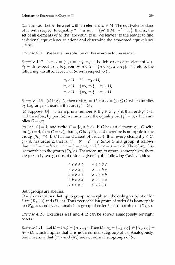
Solutions to Exercises in Chapter II 259
Exercise 4.6. Let M be a set with an element m ∈ M. The equivalence classof m with respect to equality “=” is Mm = {m′ ∈ M | m′ = m}, that is, theset of all elements of M that are equal to m. We leave it to the reader to findadditional equivalence relations and determine the associated equivalenceclasses.
Exercise 4.11. We leave the solution of this exercise to the reader.
Exercise 4.12. Let U = 〈π4〉 = {π1, π4}. The left coset of an element π ∈S3 with respect to U is given by π ◦ U = {π ◦ π1, π ◦ π4}. Therefore, thefollowing are all left cosets of S3 with respect to U:
π1 ◦U = U = π4 ◦U,π2 ◦U = {π2, π6} = π6 ◦U,π3 ◦U = {π3, π5} = π5 ◦U.
Exercise 4.15. (a) If g ∈ G, then ord(g) = |U| for U = 〈g〉 ≤ G, which impliesby Lagrange’s theorem that ord(g) | |G|.(b) Suppose |G| = p for a prime number p. If g ∈ G, g 6= e, then ord(g) > 1,and therefore, by part (a), we must have the equality ord(g) = p, which im-plies G = 〈g〉.(c) Let |G| = 4, and write G = {e, a, b, c}. If G has an element g ∈ G withord(g) = 4, then G = 〈g〉, that is, G is cyclic, and therefore isomorphic to thegroup (R4,⊕). If G has no element of order 4, then every element g ∈ G,g 6= e, has order 2, that is, a2 = b2 = c2 = e. Since G is a group, it followsthat a ◦ b = c = b ◦ a, a ◦ c = b = c ◦ a, and b ◦ c = a = c ◦ b. Therefore, G isisomorphic to the group (D4, ◦). Therefore, up to group isomorphism, thereare precisely two groups of order 4, given by the following Cayley tables:
◦ e a b ce e a b ca a b c eb b c e ac c e a b
◦ e a b ce e a b ca a e c bb b c e ac c b a e
Both groups are abelian.One shows further that up to group isomorphism, the only groups of order6 are (R6,⊕) and (D6, ◦). Thus every abelian group of order 6 is isomorphicto (R6,⊕), and every nonabelian group of order 6 is isomorphic to (D6, ◦).
Exercise 4.19. Exercises 4.11 and 4.12 can be solved analogously for rightcosets.
Exercise 4.21. Let U = 〈π4〉= {π1, π4}. Then U ◦π2 = {π2, π5} 6= {π2, π6}=π2 ◦U, which implies that U is not a normal subgroup of S3. Analogously,one can show that 〈π5〉 and 〈π6〉 are not normal subgroups of S3.
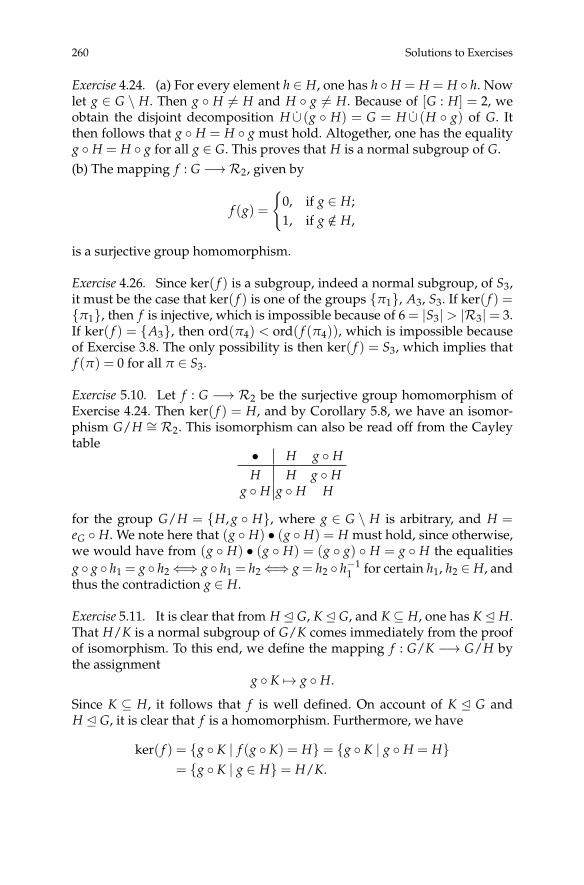
260 Solutions to Exercises
Exercise 4.24. (a) For every element h ∈ H, one has h ◦ H = H = H ◦ h. Nowlet g ∈ G \ H. Then g ◦ H 6= H and H ◦ g 6= H. Because of [G : H] = 2, weobtain the disjoint decomposition H ∪ (g ◦ H) = G = H ∪ (H ◦ g) of G. Itthen follows that g ◦ H = H ◦ g must hold. Altogether, one has the equalityg ◦ H = H ◦ g for all g ∈ G. This proves that H is a normal subgroup of G.(b) The mapping f : G −→R2, given by
f (g) =
{0, if g ∈ H;1, if g /∈ H,
is a surjective group homomorphism.
Exercise 4.26. Since ker( f ) is a subgroup, indeed a normal subgroup, of S3,it must be the case that ker( f ) is one of the groups {π1}, A3, S3. If ker( f ) ={π1}, then f is injective, which is impossible because of 6 = |S3|> |R3|= 3.If ker( f ) = {A3}, then ord(π4) < ord( f (π4)), which is impossible becauseof Exercise 3.8. The only possibility is then ker( f ) = S3, which implies thatf (π) = 0 for all π ∈ S3.
Exercise 5.10. Let f : G −→ R2 be the surjective group homomorphism ofExercise 4.24. Then ker( f ) = H, and by Corollary 5.8, we have an isomor-phism G/H ∼= R2. This isomorphism can also be read off from the Cayleytable
• H g ◦ HH H g ◦ H
g ◦ H g ◦ H H
for the group G/H = {H, g ◦ H}, where g ∈ G \ H is arbitrary, and H =eG ◦ H. We note here that (g ◦ H) • (g ◦ H) = H must hold, since otherwise,we would have from (g ◦ H) • (g ◦ H) = (g ◦ g) ◦ H = g ◦ H the equalitiesg ◦ g ◦ h1 = g ◦ h2⇐⇒ g ◦ h1 = h2⇐⇒ g = h2 ◦ h−1
1 for certain h1, h2 ∈ H, andthus the contradiction g ∈ H.
Exercise 5.11. It is clear that from H E G, K E G, and K ⊆ H, one has K E H.That H/K is a normal subgroup of G/K comes immediately from the proofof isomorphism. To this end, we define the mapping f : G/K −→ G/H bythe assignment
g ◦ K 7→ g ◦ H.
Since K ⊆ H, it follows that f is well defined. On account of K E G andH E G, it is clear that f is a homomorphism. Furthermore, we have
ker( f ) = {g ◦ K | f (g ◦ K) = H} = {g ◦ K | g ◦ H = H}= {g ◦ K | g ∈ H} = H/K.
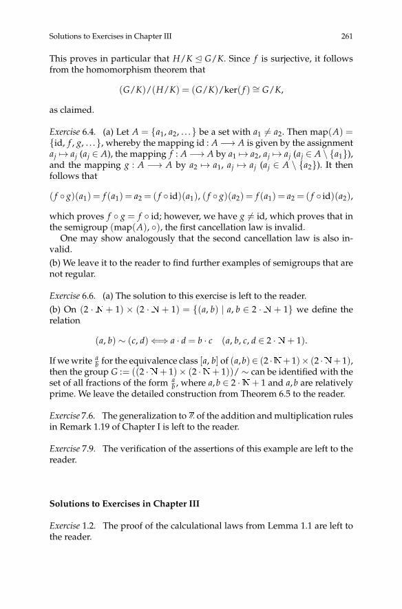
Solutions to Exercises in Chapter III 261
This proves in particular that H/K E G/K. Since f is surjective, it followsfrom the homomorphism theorem that
(G/K)/(H/K) = (G/K)/ker( f ) ∼= G/K,
as claimed.
Exercise 6.4. (a) Let A = {a1, a2, . . .} be a set with a1 6= a2. Then map(A) ={id, f , g, . . .}, whereby the mapping id : A−→ A is given by the assignmentaj 7→ aj (aj ∈ A), the mapping f : A−→ A by a1 7→ a2, aj 7→ aj (aj ∈ A \ {a1}),and the mapping g : A −→ A by a2 7→ a1, aj 7→ aj (aj ∈ A \ {a2}). It thenfollows that
( f ◦ g)(a1) = f (a1) = a2 = ( f ◦ id)(a1), ( f ◦ g)(a2) = f (a1) = a2 = ( f ◦ id)(a2),
which proves f ◦ g = f ◦ id; however, we have g 6= id, which proves that inthe semigroup (map(A), ◦), the first cancellation law is invalid.
One may show analogously that the second cancellation law is also in-valid.(b) We leave it to the reader to find further examples of semigroups that arenot regular.
Exercise 6.6. (a) The solution to this exercise is left to the reader.(b) On (2 ·N + 1) × (2 ·N + 1) = {(a, b) | a, b ∈ 2 ·N + 1} we define therelation
(a, b) ∼ (c, d)⇐⇒ a · d = b · c (a, b, c, d ∈ 2 ·N+ 1).
If we write ab for the equivalence class [a, b] of (a,b)∈ (2 ·N+ 1)× (2 ·N+ 1),
then the group G := ((2 ·N+ 1)× (2 ·N+ 1))/∼ can be identified with theset of all fractions of the form a
b , where a,b ∈ 2 ·N+ 1 and a,b are relativelyprime. We leave the detailed construction from Theorem 6.5 to the reader.
Exercise 7.6. The generalization toZ of the addition and multiplication rulesin Remark 1.19 of Chapter I is left to the reader.
Exercise 7.9. The verification of the assertions of this example are left to thereader.
Solutions to Exercises in Chapter III
Exercise 1.2. The proof of the calculational laws from Lemma 1.1 are left tothe reader.

262 Solutions to Exercises
Exercise 1.5. The proof of Theorem 1.4 is left to the reader.
Exercise 1.9. We give an idea of the proof. We assume that
a = e · p1 · · · pr = e · q1 · · ·qs
for e ∈ {±1} and for prime numbers p1, . . . , pr, q1, . . . ,qs (r ∈ N, s ∈ N), notnecessarily distinct. Since now we have p1 | a and therefore p1 | e · q1 · · ·qs, itfollows with the help of Euclid’s lemma, Lemma 1.7, that p1 | qj for some j =1, . . . , s. Since p1 is prime, we must have p1 = qj. Without loss of generality,we may assume (by renumbering if necessary) that p1 = q1. Application ofthe cancellation law implies the equality
p2 · · · pr = q2 · · ·qs. (3)
Since p2 divides the left-hand side of (3), p2 must also divide the right-handside. As in the first step, we conclude that p2 = q2. Proceeding in this way,we obtain the equalities r = s and pj = qj for j = 1, . . . ,r, which proves theasserted uniqueness.
Exercise 2.5. We leave it to the reader to prove that the polynomial ring(R[X],+, ·) is a commutative ring if and only if (R,+, ·) is commutative.
Exercise 2.6. Let A be a nonempty set and (R,+R, ·R) a ring. Then, 0R ∈ R,and therefore, the mapping 0 : A−→ R, a 7→ 0R, is an element of map(A, R).Hence, the set map(A, R) is not empty. We now show that + on map(A, R)is associative. To this end, let f , g, h∈map(A, R). Then for all a∈ A, we have
(( f + g) + h)(a) =def of +
( f + g)(a) +R h(a) =def of +
( f (a) +R g(a)) +R h(a)
=+R associative,since R is a ring
f (a) +R (g(a) +R h(a))
=def of +
f (a) +R (g + h)(a) =def of +
( f + (g + h))(a),
which proves that + is associative. The mapping 0 : A −→ R is the identityelement with respect to +, since for all f ∈map(A, R), we have the equality
(0 + f )(a) =def. of +
0(a) +R f (a) =def. of 0
0R +R f (a) =0R id. el.w.r.t. +R
f (a)
and analogously the equality ( f + 0)(a) = f (a) for all a ∈ A. The other ringproperties of map(A, R) are proved similarly using the ring properties of R.
Exercise 2.7. The solution of this exercise is left to the reader.

Solutions to Exercises in Chapter III 263
Exercise 2.11. If n > 1 is not prime, then there exist natural numbers a, b ∈Rn, a > 1, b > 1, with a · b = n. But then we have a� b = 0. Therefore, a andb are zero divisors ofRn.
Exercise 2.12. We show here only that the lack of zero divisors in (R,+, ·)implies the lack of zero divisors in (R[X],+, ·). We assume that the ring R[X]has zero divisors and show that then the ring R must have zero divisors. Let,then, f (X) = an · Xn + · · ·+ a1 · X + a0 (an 6= 0) and g(X) = bm · Xm + · · ·+b1 · X + b0 (bm 6= 0) be zero divisors in R[X], so that
f (X) · g(X) = (an · bm) · Xn+m + · · ·+ (a1 · b0 + a0 · b1) · X + a0 · b0 = 0,
where 0 denotes the zero element of R[X], i.e., the zero polynomial. In par-ticular, we must have an · bm = 0, which proves that R has zero divisors.
Exercise 2.13. The ring (map(A, R),+, ·) from Exercise 2.6 has as its zeroelement 0 : A −→ R, a 7→ 0R. If now, for example, we have R = (R6,⊕,�),then for f : A −→ R, a 7→ 2 (a ∈ A) and g : A −→ R, a 7→ 3 (a ∈ A), we havethe equality
( f · g)(a) =def of ·
f (a)� g(a) =def of f , g
2� 3 = 0 = 0(a),
that is, f and g are zero divisors of (map(A, R),+, ·). Therefore, the ring(map(A, R),+, ·) also has zero divisors if R has zero divisors. We note thatthe ring (map(A, R),+, ·) can possess zero divisors even if R has no zerodivisors.
Exercise 2.19. In the polynomial ring (Z[X],+, ·), the unit element is givenby the unit polynomial 1. Let f (X) = an · Xn + · · ·+ a1 · X + a0 (an 6= 0) be aunit in Z[X]. Then there exists a polynomial g(X) = bm · Xm + · · ·+ b1 · X +b0 (bm 6= 0) in Z[X] such that
f (X) · g(X) = (an · bm) · Xn+m + · · ·+ (a1 · b0 + a0 · b1) · X + a0 · b0 = 1.
If n > 0, then we must have in particular that an · bm = 0, in contradictionto the fact that Z has no zero divisors. Therefore, f and hence g must beof the form f (X) = a0 and g(X) = b0. The equality a0 · b0 = 1 shows that fand g are units if and only if a0 ∈ {1,−1} and a0 = b0. The polynomial ring(Z[X],+, ·) has therefore only the units {1,−1}.
Exercise 2.20. That the units of a ring (R,+, ·) with unit element 1 form agroup under multiplication with multiplicative identity element 1 followsdirectly from how units are defined.
Exercise 2.21. The group of units of R5 is (R5 \ {0},�) and is thereforeisomorphic to the group (R4,⊕). The group of units ofR8 is ({1, 3, 5, 7},�).
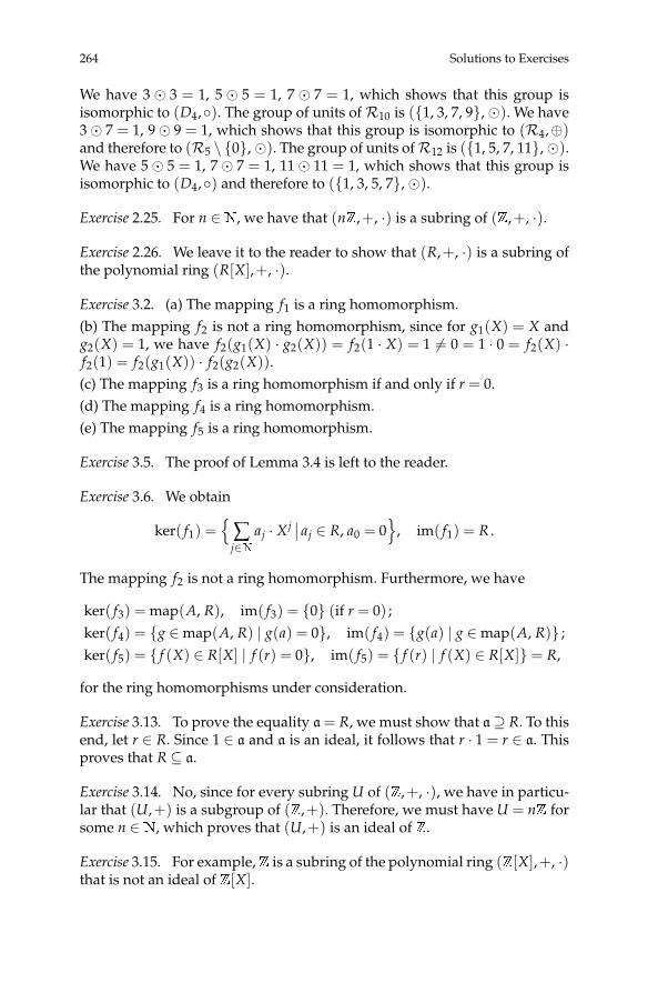
264 Solutions to Exercises
We have 3 � 3 = 1, 5 � 5 = 1, 7 � 7 = 1, which shows that this group isisomorphic to (D4,◦). The group of units ofR10 is ({1, 3, 7, 9},�). We have3� 7 = 1, 9� 9 = 1, which shows that this group is isomorphic to (R4,⊕)and therefore to (R5 \ {0},�). The group of units ofR12 is ({1, 5, 7, 11},�).We have 5� 5 = 1, 7� 7 = 1, 11� 11 = 1, which shows that this group isisomorphic to (D4,◦) and therefore to ({1, 3, 5, 7},�).
Exercise 2.25. For n ∈N, we have that (nZ,+, ·) is a subring of (Z,+, ·).
Exercise 2.26. We leave it to the reader to show that (R,+, ·) is a subring ofthe polynomial ring (R[X],+, ·).
Exercise 3.2. (a) The mapping f1 is a ring homomorphism.(b) The mapping f2 is not a ring homomorphism, since for g1(X) = X andg2(X) = 1, we have f2(g1(X) · g2(X)) = f2(1 · X) = 1 6= 0 = 1 · 0 = f2(X) ·f2(1) = f2(g1(X)) · f2(g2(X)).(c) The mapping f3 is a ring homomorphism if and only if r = 0.(d) The mapping f4 is a ring homomorphism.(e) The mapping f5 is a ring homomorphism.
Exercise 3.5. The proof of Lemma 3.4 is left to the reader.
Exercise 3.6. We obtain
ker( f1) ={
∑j∈N
aj · X j ∣∣ aj ∈ R, a0 = 0}
, im( f1) = R .
The mapping f2 is not a ring homomorphism. Furthermore, we have
ker( f3) = map(A, R), im( f3) = {0} (if r = 0) ;ker( f4) = {g ∈map(A, R) | g(a) = 0}, im( f4) = {g(a) | g ∈map(A, R)} ;ker( f5) = { f (X) ∈ R[X] | f (r) = 0}, im( f5) = { f (r) | f (X) ∈ R[X]} = R,
for the ring homomorphisms under consideration.
Exercise 3.13. To prove the equality a= R, we must show that a⊇ R. To thisend, let r ∈ R. Since 1 ∈ a and a is an ideal, it follows that r · 1 = r ∈ a. Thisproves that R ⊆ a.
Exercise 3.14. No, since for every subring U of (Z,+, ·), we have in particu-lar that (U,+) is a subgroup of (Z,+). Therefore, we must have U = nZ forsome n ∈N, which proves that (U,+) is an ideal of Z.
Exercise 3.15. For example,Z is a subring of the polynomial ring (Z[X],+, ·)that is not an ideal of Z[X].

Solutions to Exercises in Chapter III 265
Exercise 3.16. The principal ideals of Z[X] are of the form {h · f | f ∈ Z[X]}for some h ∈ Z[X]. We leave it to the reader to show that the ideal
a := {2 · f + X · g | f , g ∈ Z[X]}
is not a principal ideal of (Z[X],+, ·).
Exercise 3.18. We have ker( f1) = (X) and ker( f5) = (X − r). If the ring Rpossesses a unit element, then ker( f3) = (1).
Exercise 3.27. Let a ∈ Z. Then the mapping f : Z[X] −→ Z given by the as-signment f (X) 7→ f (a) is a surjective ring homomorphism with ker( f ) =(X − a) by Exercises 3.2, 3.6, and 3.18. Invoking Corollary 3.25, we see thatZ[X]/(X− a) ∼= Z is a ring isomorphism, as desired.
Exercise 3.28. An analogy to the group isomorphism from Exercise 5.11 ofChapter II can also be formulated and proved for rings by replacing “sub-group” and “normal subgroup” throughout with “ideal” and observing thatthe group homomorphisms that arise are also ring homomorphisms. Weleave this task to the reader.
Exercise 4.4. This is impossible, since one can show that every skew fieldwith finitely many elements is in fact a field.
Exercise 5.3. The proofs of associativity of ⊕, commutativity of �, and thesecond distributive law are left to the reader.
Exercise 5.5. We consider the ring homomorphism f : K −→Quot(K) givenby a 7→ [a, 1]. The ring homomorphism f is well defined, since K is a field,and therefore, we have 1 ∈ K. Moreover, f is injective, which can be shownas follows: Assume that [a, 1] = [b, 1] for a, b ∈ K. Then (a, 1)∼ (b, 1), whichimplies a · 1 = 1 · b and hence a = b. We now show that f is also surjective.To this end, let [a, b] ∈Quot(K) with a, b ∈ K, b 6= 0, be an arbitrary element.Since K is a field, there exists an inverse b−1 ∈ K to b. Therefore, we havea · b−1 ∈ K and
f (a · b−1) = [a · b−1, 1] = [a, b],
where the last equality follows from (a · b−1, 1) ∼ (a, b) ⇐⇒ a · b−1 · b =1 · a⇐⇒ a = a. Therefore, f is a ring isomorphism, and we have the ringisomorphism K ∼= Quot(K).
Exercise 6.3. Let r = s/t for s ∈ Z and t ∈N \ {0}. Then r corresponds to theelement [s, t] ∈ Z× (Z \ {0}). If now d = (s, t) > 0 is the greatest commondivisor of s and t, then we may write s = d · a and t = d · b with a ∈ Z,b ∈ N \ {0}, and a, b relatively prime. From the equality s · b = (d · a) · b =(d · b) · a = t · a we infer the equality [s, t] = [a, b]. This proves the existence

266 Solutions to Exercises
of the claimed representative. To prove the uniqueness of the representative,we assume that [c, d] with c ∈Z, d ∈N \ {0}, and c, d relatively prime is alsoan element such that [s, t] = [c, d]. Then in particular, we have [a, b] = [c, d],and therefore
a · d = b · c.
If p is a prime number such that p | a, then we must have p | b · c and conse-quently, since p is prime, p | b or p | c. But since a and b are relatively prime,we must have p | c. Conversely, one can show that for an arbitrary prime pwith p | c, we must also have p | a. From this it follows that a | c and also c | a,which, since a and c have the same sign, proves the equality a = c. We con-clude by an analogous argument the equality b = d, completing the proof ofuniqueness.
Exercise 6.4. Since one usually learns this proof in a first course in real anal-ysis, we leave this exercise to the reader.
Exercise 6.7. The generalizations of the addition and multiplication rulesfrom Remark 1.19 of Chapter I are left to the reader.
Exercise 7.4. We obtain in Z[X] the decompositions 20X = 22 · 5 · X and10X2 + 4X − 6 = 2 · (X + 1) · (5X − 3). Therefore, 2 is the greatest commondivisor, and 22 · 5 · X · (X + 1) · (5X − 3) = 100X3 + 40X2 − 60X the leastcommon multiple, of the polynomials 20X and 10X2 + 4X− 6 in Z[X].
Exercise 7.9. We leave it to the reader to come up with relevant examples.
Exercise 7.15. Part (ii) of the proof of Lemma 7.14 is left to the reader.
Exercise 7.25. For example, the polynomial ring K[X,Y] in two variablesover a field K is not a principal ideal domain, since the ideal
a := {X · f + Y · g | f , g ∈ K[X,Y]}
is not principal.
Exercise 7.38. (a) We obtain (123456789,555555555) = 9.(b) We calculate
X4 + 2X3 + 2X2 + 2X + 1 = (X + 1) · (X3 + X2 − X− 1) + (2X2 + 4X + 2) ,
X3 + X2 − X− 1 =(1
2X− 1
2
)· (2X2 + 4X + 2) + 0.
We thereby obtain (X4 + 2X3 + 2X2 + 2X + 1, X3 + X2 − X − 1) = 2X2 +4X + 2.
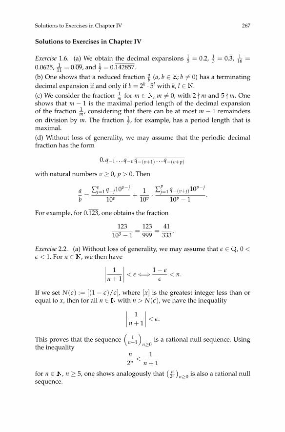
Solutions to Exercises in Chapter IV 267
Solutions to Exercises in Chapter IV
Exercise 1.6. (a) We obtain the decimal expansions 15 = 0.2, 1
3 = 0.3, 116 =
0.0625, 111 = 0.09, and 1
7 = 0.142857.(b) One shows that a reduced fraction a
b (a, b ∈ Z; b 6= 0) has a terminatingdecimal expansion if and only if b = 2k · 5l with k, l ∈N.(c) We consider the fraction 1
m for m ∈ N, m 6= 0, with 2 - m and 5 - m. Oneshows that m − 1 is the maximal period length of the decimal expansionof the fraction 1
m , considering that there can be at most m − 1 remainderson division by m. The fraction 1
7 , for example, has a period length that ismaximal.(d) Without loss of generality, we may assume that the periodic decimalfraction has the form
0.q−1 . . . q−v q−(v+1) . . . q−(v+p)
with natural numbers v ≥ 0, p > 0. Then
ab=
∑vj=1 q−j10v−j
10v +1
10v ·∑
pj=1 q−(v+j)10p−j
10p − 1.
For example, for 0.123, one obtains the fraction
123103 − 1
=123999
=41
333.
Exercise 2.2. (a) Without loss of generality, we may assume that ε ∈Q, 0 <ε < 1. For n ∈N, we then have∣∣∣∣ 1
n + 1
∣∣∣∣ < ε⇐⇒ 1− ε
ε< n.
If we set N(ε) := [(1− ε)/ε], where [x] is the greatest integer less than orequal to x, then for all n ∈Nwith n > N(ε), we have the inequality∣∣∣∣ 1
n + 1
∣∣∣∣ < ε.
This proves that the sequence(
1n+1
)n≥0
is a rational null sequence. Usingthe inequality
n2n <
1n + 1
for n ∈N, n ≥ 5, one shows analogously that( n
2n
)n≥0 is also a rational null
sequence.

268 Solutions to Exercises
(b) Other examples of rational null sequences are the sequences(
1(n+1)k
)n≥0with k ∈N, k ≥ 2.
Exercise 2.18. Let α = (an) + n, β = (bn) + n be two real numbers with α <β, that is, there exist q ∈ Q, q > 0, N(q) ∈ N with bn − an > q for all n ∈N with n > N(q). To prove the asserted independence of the choice of therepresenting rational Cauchy sequences, we assume that (an) + n= (a′n) + nand (bn) + n = (b′n) + n for rational Cauchy sequences (a′n) and (b′n). Thenin particular, we must have (a′n) = (an) + (cn) = (an + cn) and (b′n) = (bn) +(dn) = (bn + dn) for rational null sequences (cn) and (dn). This yields
b′n − a′n = (bn − an) + (dn − cn) ≥ (bn − an)− |dn − cn|. (4)
Since, moreover, (dn − cn) is a rational null sequence, there exists for ε :=q/2 ∈ Q an N(ε) ∈ N such that for all n ∈ N with n > N(ε), we have theinequality |dn − cn| < ε. So if we set q′ := q− ε = q/2 ∈Q, we have q′ > 0,and with (4) we obtain the inequality
b′n − a′n > q− ε = q′
for all n ∈ N with n > N(q′) := max(N(q), N(ε)). This proves the claimedindependence of representative.
Exercise 2.22. We leave the proof of Lemma 2.21 to the reader.
Exercise 2.25. Real null sequences whose elements are irrational numbersinclude, for example, the sequences
( √2
(n+1)k
)n≥0
with k ∈N, k ≥ 1.
Exercise 2.30. We begin by considering that for a rational number a0 ∈ Q,a0 > 0, we have the following equivalences with an error of δ0:
a0 + δ0 =√
2⇐⇒ (a0 + δ0)2 = 2⇐⇒ 2a0δ0 + δ2
0 = 2− a20
⇐⇒ δ0 =2− a2
02a0
− δ20
2a0.
So if we set
a1 := a0 +2− a2
02a0
=2 + a2
02a0
,
then because a0 > 0, we have the inequality a21 > 2, that is, a1 >
√2. This
implies(2− a2
1)/(2a1) < 0, and we therefore have for
a2 := a1 +2− a2
12a1
=2 + a2
12a1

Solutions to Exercises in Chapter IV 269
both a1 > a2 and a22 > 2, that is, a2 >
√2. We consider now the rational se-
quence (an)n≥0 with a0 ∈Q, a0 > 0, arbitrary and
an+1 :=2 + a2
n2an
(n ∈N,n ≥ 1). (5)
One first shows by induction that both an > an+1 for all n ∈ N, n ≥ 1, anda2
n > 2, that is, an >√
2, for all n ∈ N, n ≥ 1. Using these inequalities, onethen shows in a second step that (an)n≥0 is a rational Cauchy sequence. Thisrational Cauchy sequence has limit α ∈ R, α > 0. Because of the recurrenceformula (5), we see that α satisfies the equation
α =2 + α2
2α⇐⇒ α =
√2,
as desired.
Exercise 3.12. (a) The decimal representation 0.101001000100001 . . . is nei-ther terminating nor periodic. Therefore, this number cannot be rational.One can find analogous examples, such as 0.121331222133331 . . . .(b) Using the rational Cauchy series (an)n≥0 constructed in Exercise 2.30for calculating
√2, one obtains
√2 ≈ 1.4142135623, accurate to ten decimal
places, by choosing, for example, a0 = 1 and iterating four times.
Exercise 4.2. We consider, for example, the sequence
(an)n≥0 :=(
n2 + 22n
)n≥0
.
We have a0 = 2 and a1 = a2 = 3/2. For n∈N, n≥ 3, one shows the inequality2(n2 + 2) > (n + 1)2 + 2. Since
2(n2 + 2) > (n + 1)2 + 2⇐⇒ n2 + 22n >
(n + 1)2 + 22n+1 ⇐⇒ an > an+1
for n ∈ N, n ≥ 3, it follows that the sequence (an)n≥0 is monotonically de-creasing, but not strictly. One shows analogously that the sequences(
121
n+1
)n≥0
,(
n3 + 33n
)n≥0
are strictly monotonically decreasing and that the sequence(n3 − 2n2 − 2
)n≥0

270 Solutions to Exercises
is monotonically increasing. The sequence(n
1n+1
)n≥0
is neither monotonically increasing nor monotonically decreasing. How-ever, the sequence (
n1
n+1
)n≥4
is strictly monotonically decreasing.
Exercise 4.6. The subset M ⊆Q consisting of all sequence terms an (n > 0)in the rational Cauchy sequence (an)n≥0 constructed in Exercise 2.30, whichis bounded below, has greatest lower bound
√2 /∈Q.
Exercise 4.7. The greatest lower bound of the set { x√
x | x ∈Q, x ≥ 0} is at-tained when x = 0 and is equal to zero. The least upper bound is e
√e.
Exercise 5.3. The solution of this exercise is left to the reader.
Exercise 6.7. We leave the completion of the details in the sketch of the proofof Theorem 6.5 to the reader.
Solutions to Exercises in Chapter V
Exercise 1.1. The solution of this exercise is left to the reader.
Exercise 1.8. The completion of the proof of Theorem 1.7 is left to the reader.
Exercise 1.10. Let α = α1 + α2i∈C, α 6= 0. If α2 = 0 and α1 > 0, then±√α1 arethe solutions to the equation x2 = α. If α2 = 0 and α1 < 0, then ±
√|α1|i are
the solutions to the equation x2 = α. It remains to consider the case α2 6= 0.Let β = β1 + β2i ∈Cwith β1 6= 0. We then have the equivalence
β2 = α⇐⇒ (β21 − β2
2) + (2β1β2)i = α1 + α2i⇐⇒ β21 − β2
2 = α1, 2β1β2 = α2.
If we substitute the second equation, β2 = α2/(2β1), in the first equation,we obtain the equation 4β4
1 − 4α1β21 − α2
2 = 0. Setting y := β21, we obtain the
quadratic equation 4y2 − 4α1y− α22 = 0, which has the solutions
y1,2 =α1 ±
√α2
1 + α22
2=
α1 ± |α|2
.

Solutions to Exercises in Chapter V 271
Since now β1 ∈R, we need consider only the nonnegative solution y1. Withβ1 = ±
√y1 and β2 = ±α2/(2
√y1), we obtain the solution formula
β = ±√
α1 + |α|√2
± α2i√2(α1 + |α|
) .
Altogether, we obtain for the solutions to the equation x2 = α the followingsolution formula:
x1,2 =
±√α1 , if α1 > 0, α2 = 0;
±√|α1| i , if α1 < 0, α2 = 0;
±(√ |α|+α1
2 +√|α|−α1
2 i)
, if α2 > 0;
±(√ |α|+α1
2 −√|α|−α1
2 i)
, if α2 < 0.
From this it follows that the solutions to the equation x2 = i are
x1,2 = ±1 + i√
2,
those to the equation x2 = 2 + i are
x1,2 = ±(√√
5 + 2√2
+
√√5− 2√2
i)
,
and those to the equation x2 = 3− 2i are
x1,2 = ±(√√
13 + 3√2
−√√
13− 3√2
i)
.
Exercise 1.11. Since by Exercise 1.10 we have the equality ((1+ i)/2)2 = i/2,we obtain, on completing the square,
x2 + (1 + i) · x + i = 0⇐⇒(
x +1 + i
2
)2+
i2= 0.
If we now substitute y := x + (1 + i)/2, we obtain the quadratic equationy2 = −i/2. With the solution formula from Exercise 1.10, we obtain the so-lution
x1,2 = y1,2 −1 + i
2= ±1
2∓ i
2− 1 + i
2,
that is, x1 =−i and x2 =−1 are the solutions of x2 + (1+ i) · x + i = 0, whichcan be easily checked by substitution. One can prove analogously that theequation x2 + (2− i) · x− 2i = 0 has the solutions x1 = i and x2 = −2.

272 Solutions to Exercises
Exercise 1.14. (a) First, one verifies the equality α · β = α · β for all α, β ∈C.One then has
|α · β|2 = (α · β) · α · β = α · α · β · β = |α|2 · |β|2,
which proves the assertion.(b) Let α1, α2, β1, β2 ∈ N. The product rule from part (a) with α = α1 + α2iand β = β1 + β2i yields
(α21 + α2
2) · (β21 + β2
2) = (α1β1 − α2β2)2 + (α1β2 + α2β1)
2.
This implies the assertion.
Exercise 2.3. The statement of Remark 2.2 results immediately from use ofthe product rule from Exercise 1.14.
Exercise 2.5. Let A ∈M2(R) be an invertible matrix. One may convince one-self that the mapping fA : (C, +, ·) −→ (M2(R), +, ·) given by
α = α1 + α2i 7→ A ·(
α1 α2−α2 α1
)· A−1
is an injective ring homomorphism. In particular, f induces an isomorphismC∼= im( f ), that is, C is isomorphic to the subring im( f ) of M2(R).
Exercise 2.8. The solution of this exercise is left to the reader.
Exercise 2.12. We first observe that for two complex numbers α, β ∈C \ {0} with polar coordinate representations α = |α| · (cos(ϕ) + i sin(ϕ))and β = |β| · (cos(ψ) + i sin(ψ)), one has the following multiplication for-mula:
α · β = |α||β| ·(cos(ϕ)cos(ψ)− sin(ϕ)sin(ψ)
+ i(sin(ϕ)cos(ψ) + cos(ϕ)sin(ψ)
))= |α||β| ·
(cos(ϕ + ψ) + i sin(ϕ + ψ)
),
where for the second equality we have invoked the addition theorems forsine and cosine. From this follows for m ∈N the equality
αm = |α|m ·(cos(mϕ) + i sin(mϕ)
).
Likewise, for n ∈Nwith n 6= 0, we obtain the equality
α1n = |α| 1n ·
(cos( ϕ
n
)+ i sin
( ϕ
n
)).
This completes the proof of the general formula.

Solutions to Exercises in Chapter VI 273
Exercise 4.4. Let p be a prime number. Then f (X) = X2 − p is a quadraticpolynomial with integer coefficients, and we have f (
√p) = 0. We now as-
sume that there exists a linear polynomial g(X) = aX + b (a, b ∈ Z, a 6= 0)with g(
√p) = 0. But then we must have
√p = −b/a ∈ Q, a contradiction.
We have therefore shown that√
p is algebraic of degree 2.
Exercise 4.12. We leave it to the reader to find additional transcendentalnumbers following the pattern of the Liouville number.
Exercise 5.8. The calculation of better approximations to e is left to thereader.
Solutions to Exercises in Chapter VI
Exercise 1.6. For example, the quadratic polynomial X2 + 1∈H[X] has zeros±i,±j,±k and every purely imaginary quaternion α2i + α3 j + α4k ∈ Im(H),that satisfies the condition α2
2 + α23 + α2
4 = 1.
Exercise 1.7. It is clear that R ⊆ Z(H). We therefore have to show thatZ(H) ⊆ R. To this end, let α = α1 + α2i + α3 j + α4k ∈ Z(H). For each β =β1 + β2i + β3 j + β4k ∈H, we then have α · β = β · α. Since
α · β = (α1β1 − α2β2 − α3β3 − α4β4) + (α1β2 + α2β1 + α3β4 − α4β3)i+ (α1β3 − α2β4 + α3β1 + α4β2)j + (α1β4 + α2β3 − α3β2 + α4β1)k
and
β · α = (β1α1 − β2α2 − β3α3 − β4α4) + (β1α2 + β2α1 + β3α4 − β4α3)i+ (β1α3 − β2α4 + β3α1 + β4α2)j + (β1α4 + β2α3 − β3α2 + β4α1)k,
however, we have
α · β = β · α⇐⇒ 2(α3β4 − α4β3)i + 2(−α2β4 + α4β2)j + 2(α2β3 − α3β2)k = 0⇐⇒ α3β4 = α4β3 ∧ α4β2 = α2β4 ∧ α2β3 = α3β2.
If α2 6= 0, then from the third equality, it follows that β3 = (α3α−12 ) · β2 for
every β ∈H. This contradiction implies that we must have α2 = 0. Similarly,one shows that we must also have α3 = 0 and α4 = 0. Altogether, therefore,we have that α = α1 ∈R. This proves the inclusion Z(H) ⊆R.
Exercise 1.14. (a) Let α = α1 + α2i + α3 j + α4k. We then calculate

274 Solutions to Exercises
α2 = (α21 − α2
2 − α23 − α2
4) + 2α1α2i + 2α1α3 j + 2α1α4k
= −(α21 + α2
2 + α23 + α2
4) + 2α1α,
which yields the desired result.(b) This can be established by a direct calculation.
Exercise 1.15. Let α = Im(α) · i with Im(α) = (α2,α3,α4) and β = Im(β) · iwith Im(β) = (β2, β3, β4). We calculate
α · β = (α2i + α3 j + α4k) · (β2i + β3 j + β4k)= (−α2β2 − α3β3 − α4β4) + (α3β4 − α4β3)i+ (−α2β4 + α4β2)j + (α2β3 − α3β2)k
= −⟨Im(α)t, Im(β)t⟩+ (Im(α)t × Im(β)t) · i,
which proves the assertion.
Exercise 1.18. Let α, β ∈H. We calculate
2 · 〈α, β〉 = 2 · Re(α · β) = α · β + α · β = α · β + β · α.
Multiplication of this equality on the right by β yields
2 · 〈α, β〉 · β = α · β · β + β · α · β,
which on account of β · β = 〈β, β〉 ∈R proves the result.
Exercise 1.19. (a) The equality α · β = β · α can be verified by a direct calcu-lation.(b) Using part (a), one obtains
|α · β|2 = (α · β) · α · β = α · (β · β) · α = |β|2 · (α · α) = |β|2 · |α|2 = |α|2 · |β|2,
which proves the assertion.(c) Let α1, α2, α3, α4, β1, β2, β3, β4 ∈N. Using the product rule from part (a),we obtain
(α21 + α2
2 + α23 + α2
4) · (β21 + β2
2 + β23 + β2
4)
= (α1β1 − α2β2 − α3β3 − α4β4)2 + (α1β2 + α2β1 + α3β4 − α4β3)
2
+ (α1β3 + α3β1 + α4β2 − α2β4)2 + (α1β4 + α4β1 + α2β3 − α3β2)
2.
This implies the assertion.
Exercise 1.21. The completion of the proof of Theorem 1.20 is left to thereader.

Solutions to Exercises in Chapter VI 275
Exercise 1.25. Verification of the assertions of this problem is left to thereader.
Exercise 1.27. The solution to this problem is left to the reader.
Exercise 2.3. The statement of Remark 2.2 is an immediate result of the prod-uct rule from Exercise 1.19.
Exercise 2.5. Let A ∈M2(C) be an arbitrary invertible matrix. One may con-vince oneself that the mapping f : (H, +, ·) −→ (M2(C), +, ·) given by
α = α1 + α2i + α3 j + α4k 7→ A ·(
α1 + α2i α3 + α4i−α3 + α4i α1 − α2i
)· A−1
is an injective ring homomorphism. In particular, f induces an isomorphismH∼= im( f ), that is,H is isomorphic to the subring im( f ) of M2(C).
Exercise 2.6. We show that f is an R-linear mapping. Let α = α1 + α2i +α3 j + α4k ∈H and β = β1 + β2i + β3 j + β4k ∈H. For arbitrary µ,ν ∈R, onehas
f (µα + νβ) = f ((µα1 + νβ1) + (µα2 + νβ2)i + (µα3 + νβ3)j + (µα4 + νβ4)k)
=
((µα1 + νβ1) + (µα2 + νβ2)i (µα3 + νβ3) + (µα4 + νβ4)i−(µα3 + νβ3) + (µα4 + νβ4)i (µα1 + νβ1)− (µα2 + νβ2)i
)= µ
(α1 + α2i α3 + α4i−α3 + α4i α1 − α2i
)+ ν
(β1 + β2i β3 + β4i−β3 + β4i β1 − β2i
)= µ f (α) + ν f (β),
that is, f is R-linear. The verification of the remaining assertions are left tothe reader.
Exercise 2.9. The solution to this problem is left to the reader.
Exercise 3.4. The solution to this problem is left to the reader.
Exercise 3.6. We first prove that every R-linear mapping v 7→ A · v (v ∈R3)with A ∈ SO3(R) is an orientation-preserving rotation of R3 about an axispassing through the origin. To this end, we begin by noting that for A ∈SO3(R), on account of
det(A− E) = 1 · det(A− E) = det(At) · det(A− E)
= det(At · (A− E)) = det(E− At) = det(E− A)t
= det(E− A) = (−1) · det(A− E),

276 Solutions to Exercises
we have the equality det(A− E) = 0, which proves that 1 is an eigenvalueof A. Now let a1 denote a normalized (to have length 1) eigenvector of Aassociated with the eigenvalue 1. We shall see that the mapping v 7→ A · v(v ∈ R3) describes a rotation about an axis passing through the origin thatis determined by a1. For this, we extend a1 to an orthonormal basis of R3
by choosing an additional vector a2 ∈ R3, normed to have length 1, that isperpendicular to a1, and then setting a3 := a1× a2. If now S∈M2(R) denotesa matrix with S · (1,0,0)t = a1, S · (0,1,0)t = a2, and S · (0,0,1)t = a3, then wemust have S ∈ SO3(R). We further obtain
S−1 · A · S · (1,0,0)t = S−1 · A · a1 = S−1 · a1 = (1,0,0)t,
which implies the equality
S−1 · A · S =
1 0 00 α β0 γ δ
for certain α, β, γ, δ ∈ R. But since because of A,S ∈ SO3(R), we have alsothe inclusion S−1 · A · S ∈ SO3(R) and thereby(
α βγ δ
)∈ SO2(R),
it follows that there exists a uniquely determined ϕ ∈ [0,2π) with
S−1 · A · S =
1 0 00 cos(ϕ) −sin(ϕ)0 sin(ϕ) cos(ϕ)
=: Dϕ.
The mapping v 7→ Dϕ · v (v ∈R3) is an orientation-preserving rotation in thex2, x3-plane through the angle ϕ about the x1-axis (counterclockwise if a1points toward the observer). Altogether, we have shown that the mappingv 7→ A · v (v ∈ R3) is an orientation-preserving rotation in the a2, a3-planethrough the angle ϕ about the a1-axis (counterclockwise if a1 points towardthe observer).
We now describe, conversely, an arbitrary orientation-preserving rotationofR3 through the angle ϕ ∈ [0,2π) about an axis passing through the originthat is determined by the vector (normed to have length 1) a1 := (ν1,ν2,ν3)
t ∈R3. To this end, we first consider the matrices
D1 :=
ν1√
ν21+ν2
30 ν3√
ν21+ν2
30 1 0
− ν3√ν2
1+ν23
0 ν1√ν2
1+ν23
, D2 :=
√
ν21 + ν2
3 ν2 0
−ν2
√ν2
1 + ν23 0
0 0 1
∈ SO3(R).

Solutions to Exercises in Chapter VI 277
If in the first step we apply D1 to a1, we rotate a1 about the x2-axis in such away that D1 · a1 lies in the x1, x2-plane. If in the second step we apply D2 toD1 · a1, then we rotate D1 · a1 about the x3-axis, so that finally, D2 · D1 · a1 isparallel to the x1-axis. Altogether, the orientation-preserving rotation underdiscussion is given by the mapping v 7→ A · v (v ∈R3) with A := D−1
1 ·D−12 ·
Dϕ · D2 · D1. Multiplying out yields
A =
ν21 µ + cos(ϕ) ν1ν2µ− ν3 sin(ϕ) ν1ν3µ + ν2 sin(ϕ)
ν1ν2µ + ν3 sin(ϕ) ν22 µ + cos(ϕ) ν2ν3µ− ν1 sin(ϕ)
ν1ν3µ− ν2 sin(ϕ) ν2ν3µ + ν1 sin(ϕ) ν23 µ + cos(ϕ)
,
where we have set µ := 1− cos(ϕ); this can now be easily decomposed as
A = E + sin(ϕ) · N + (1− cos(ϕ)) · N2
with
N :=
0 −ν3 ν2ν3 0 −ν1−ν2 ν1 0
,
as asserted.
Selected Literature
The following list of books on (elementary) number theory and algebra canserve to fill in some of the gaps in this book’s presentation. Some of thesebooks will take the reader much deeper into various topics. The literatureon the concept of number and the representation of numbers is of cultural-historical significance, while the works of a historical nature provide insightinto the historical development of algebra and number theory. Finally, weoffer the interested reader two books on approaches to the teaching of alge-bra and number theory.
Selected literature for the appendices is listed at the end of the respectiveappendix.
Literature on Number Theory
[1] D. Burton: Elementary number theory. McGraw-Hill Education, 7th edi-tion, 2010.
[2] W. A. Coppel: Number theory. An introduction to mathematics. Springer,Berlin Heidelberg New York, 2nd edition, 2009.
[3] G. H. Hardy, E. M. Wright: An introduction to the theory of numbers. Ox-ford University Press, 6th edition, 2008.
[4] H. Hasse: Number theory. Translated from the 3rd German edition. Sprin-ger, Berlin Heidelberg New York, 1980.
[5] L. -K. Hua: Intoduction to number theory. Translated from the Chineseoriginal by P. Shiu. Springer, Berlin Heidelberg New York, 1982.
[6] K. Ireland, M. Rosen: A classical introduction to modern number theory.Springer, Berlin Heidelberg New York, 2nd edition, 1990.
[7] F. Jarvis: Algebraic number theory. Springer, Cham Heidelberg New YorkDordrecht London, 2014.
[8] G. A. Jones, J. M. Jones: Elementary number theory. Springer, London,1998.
[9] M. B. Nathanson: Elementary methods in number theory. Springer, BerlinHeidelberg New York, 2000.
[10] I. Niven, H. S. Zuckerman, H. L. Montgomery: An introduction to the the-ory of numbers. John Wiley & Sons, Hoboken, NJ, 5th edition, 2008.
[11] D. Redmond: Number theory. Marcel Dekker, New York, 1996.[12] K. H. Rosen: Elementary number theory and its applications. Pearson, Bos-
ton, 6th edition, 2010.
© Springer International Publishing AG 2017
Springer Undergraduate Mathematics Series, https://doi.org/10.1007/978-3-319-69429-0J. Kramer and A.-M. von Pippich, From Natural Numbers to Quaternions,
280 Selected Literature
[13] W. Sierpinski: Elementary theory of numbers. Elsevier, Amsterdam, PWN,Warsaw, 2nd edition, 1988.
[14] A. Weil: Basic number theory. Springer, Berlin Heidelberg New York,3rd edition, 1995.
Literature on Abstract Algebra
[15] M. Artin: Algebra. Pearson, Boston, 2nd edition, 2017.[16] R. Cooke: Classical algebra: its nature, origins, and uses. John Wiley &
Sons, Hoboken, NJ, 2008.[17] D. S. Dummit, R. M. Foote: Abstract algebra. John Wiley & Sons, Hobo-
ken, NJ, 3rd edition, 2003.[18] B. Fine, A. M. Gaglione, G. Rosenberger: Introduction to abstract algebra.
Johns Hopkins University Press, Baltimore, MD, 2014.[19] J. Gallian: Contemporary abstract algebra. Brooks Cole, 9th edition, 2016.[20] R. S. Irving: Integers, polynomials, and rings. Springer, Berlin Heidelberg
New York, 2004.[21] S. Lang: Algebra. Springer, Berlin Heidelberg New York, 3rd edition,
2002.[22] F. Lorenz: Algebra. Volume I. Fields and Galois theory. Translated from the
1987 German edition by S. Levy. Springer, Berlin Heidelberg New York,2006.
[23] W. K. Nicholson: Introduction to abstract algebra. John Wiley & Sons,Hoboken, NJ, 4th edition, 2012.
[24] J. J. Rotman: A first course in abstract algebra. Pearson, Boston, 3rd edi-tion, 2005.
[25] L. H. Rowen: Algebra: groups, rings and fields. A K Peters, Wellesley, MA,1994.
[26] J. Stillwell: Elements of algebra: geometry, numbers, equations. Springer,Berlin Heidelberg New York, 1994.
[27] B. L. van der Waerden: Algebra. Volume I. Springer, Berlin HeidelbergNew York, 9th edition, 1993.
Literature on the Concept of Number
[28] J. H. Conway, R. K. Guy: The book of numbers. Springer Copernicus, NewYork, 1996.
[29] L. Corry: A brief history of numbers. Oxford University Press, Oxford,2015.
[30] H. Ebbinghaus et al.: Numbers. Translated from the 2nd German 1988edition by H. L. S. Orde. Springer, Berlin Heidelberg New York, 1991.
[31] G. Ifrah: From one to zero: a universal history of numbers. Translated fromthe French original by L. Bair. Penguin Books, New York, 1987.

281
[32] K. Menninger: Number words and number symbols: a cultural history ofnumbers. Translated from the German revised edition by P. Broneer.Dover, New York, 1992.
[33] R. Taschner: Numbers at work: a cultural perspective. Translated from the2005 German original by O. Binder and D. Sinclair-Jones. A K Peters,Wellesley, MA, 2007.
Literature on the History of Algebra and Number Theory
[34] I. G. Bashmakova, G. S. Smirnova: The beginnings and evolution of algebra.Translated from the Russian original by A. Shenitzer. Mathematical As-sociation of America, Washington, DC, 2000.
[35] V. J. Katz, K. H. Parshall: Taming the unknown: a history of algebra from an-tiquity to early twentieth century. Princeton University Press, Princeton,NJ, 2014.
[36] A. Weil: Number theory. Birkhäuser Boston, Boston, MA, 1984.
Literature on the Teaching of Algebra and Number Theory
[37] A. Arcavi, P. Drijvers, K. Stacey: The learning and teaching of algebra. IM-PACT Series, Routledge, 2016.
[38] J. D. Sally, P. J. Sally: Integers, fractions, and arithmetic: a guide for teachers.American Mathematical Society, Providence, RI, 2012.

Index
associative operation, 45
bounded set, 160
Cauchy sequenceof an ordered field, 168rational, 145real, 153
Cayley table, 51Cayley’s octonions, 231characteristic, 101completeness
axiom of geometric, 166of an ordered field, 168of real numbers, 155
completeness principle, 162complex numbers, 184
absolute value, 187complex conjugate, 186imaginary part, 184modulus, 187purely imaginary, 184real part, 184
complex plane, 184coset, 61
left, 59right, 61
decimal, 155genuine, 159infinite, 155terminating, 155
decimal expansionperiod, 143periodic, 143purely periodic, 143
Dedekind cuts, 167division with remainder, 30, 95, 125divisor, 15, 94, 120, 121
common, 15, 95, 120greatest common, 25, 97, 120, 122proper, 17trivial, 17, 95
domain, 100
elementidentity, 47inverse, 48, 101irreducible, 120left identity, 47left inverse, 48, 101prime, 121right identity, 47right inverse, 48, 101unit, 98zero, 98
equivalence class, 57equivalence relation, 57Euclid’s lemma, 23, 96Euclidean algorithm, 126
extended, 127Euclidean domain, 125exponential function, 197
field, 110absolute value, 168algebraically closed, 193archimedean, 169order, 168
field of fractions, 117fraction, 76, 118fundamental theorem
of algebra, 191of arithmetic, 22, 96
group, 48abelian/commutative, 49alternating, 68cyclic, 52dihedral, 50symmetric, 51
group homomorphism, 54group isomorphism, 54
Hamilton’s quaternions, 219homomorphism theorem
for groups, 66for rings, 108
ideal, 104
© Springer International Publishing AG 2017
Springer Undergraduate Mathematics Series, https://doi.org/10.1007/978-3-319-69429-0J. Kramer and A.-M. von Pippich, From Natural Numbers to Quaternions,

284 Index
divisibility, 121greatest common divisor, 122intersection, 122least common multiple, 122principal, 105sum, 122unit, 105zero, 105
imageof a group homomorphism, 55of a ring homomorphism, 104
index of a subgroup, 61induction, 9infimum, 161infimum principle, 162integers, 74
absolute value, 76decimal representation, 141difference, 75order, 75product, 93quotient, 118
integral domain, 100
kernelof a group homomorphism, 55of a ring homomorphism, 104
least common multiple, 26, 97, 120, 122lower bound, 160
monoid, 47multiplicative group of a ring, 111
natural numbers, 9decimal representation, 31difference, 14, 75order, 13product, 11sum, 10
nested intervals, 162nested intervals principle, 162normal subgroup, 61null sequence
rational, 145number
algebraic, 193amicable, 21Euler, 197irrational, 159Liouville, 196perfect, 20transcendental, 194
octonions, 231order
of a group, 52of an element, 53
orthogonal groupO2(R), 189O3(R), 228
Peano axioms, 9predecessor, 9prime number, 17, 95
Fermat, 19Mersenne, 19
principal ideal domain, 124
quaternions, 219conjugate quaternion, 221imaginary part, 220imaginary space, 221modulus, 221purely imaginary, 220real part, 220
quotient group, 65quotient ring, 108
R-algebra, 222associative, 222commutative, 222dimension, 222division algebra, 222R-subalgebra, 223
R-algebra homomorphism, 223rational numbers, 118
absolute value, 119decimal representation, 143order, 119
real number line, 164real numbers, 151
absolute value, 153decimal expansion, 159decimal representation, 159order, 152
real sequence(strictly) monotonically decreas-ing, 160(strictly) monotonically increasing,159convergence, 153limit, 153
relatively prime, 28pairwise, 28
ring, 97commutative, 98factorial, 123
Index 285
polynomial, 99zero, 98
ring homomorphism, 103ring isomorphism, 103
semigroup, 45abelian/commutative, 46regular, 69
skew field, 110special orthogonal group
SO2(R), 189SO3(R), 228
special unitary groupSU2(C), 225
subgroup, 53subgroup criterion, 53subring, 102subring criterion, 102successor, 9supremum, 161
supremum principle, 162
theoremGauss’s, 123Lagrange’s, 60Liouville’s, 194of Euclid, 18
unique factorization domain, 123unit, 101
imaginary, 184unitary group
U2(C), 225upper bound, 160
well-ordering principle, 14
zero divisor, 100left, 100right, 100
Top Related