


Languages
Pages
Legal


Intra- and Inter-Brain Synchronization during MusicalImprovisation on the GuitarViktor Muller*, Johanna Sanger, Ulman Lindenberger
Center for Lifespan Psychology, Max Planck Institute for Human Development, Berlin, Germany
Abstract
Humans interact with the environment through sensory and motor acts. Some of these interactions require synchronizationamong two or more individuals. Multiple-trial designs, which we have used in past work to study interbrain synchronizationin the course of joint action, constrain the range of observable interactions. To overcome the limitations of multiple-trialdesigns, we conducted single-trial analyses of electroencephalography (EEG) signals recorded from eight pairs of guitaristsengaged in musical improvisation. We identified hyper-brain networks based on a complex interplay of differentfrequencies. The intra-brain connections primarily involved higher frequencies (e.g., beta), whereas inter-brain connectionsprimarily operated at lower frequencies (e.g., delta and theta). The topology of hyper-brain networks was frequency-dependent, with a tendency to become more regular at higher frequencies. We also found hyper-brain modules thatincluded nodes (i.e., EEG electrodes) from both brains. Some of the observed network properties were related to musicalroles during improvisation. Our findings replicate and extend earlier work and point to mechanisms that enable individualsto engage in temporally coordinated joint action.
Citation: Muller V, Sanger J, Lindenberger U (2013) Intra- and Inter-Brain Synchronization during Musical Improvisation on the Guitar. PLoS ONE 8(9): e73852.doi:10.1371/journal.pone.0073852
Editor: Olaf Sporns, Indiana University, United States of America
Received December 18, 2012; Accepted July 25, 2013; Published September 10, 2013
Copyright: � 2013 Muller et al. This is an open-access article distributed under the terms of the Creative Commons Attribution License, which permitsunrestricted use, distribution, and reproduction in any medium, provided the original author and source are credited.
Funding: This work was supported by the Max Planck Society and the German Research Foundation. The funders had no role in study design, data collection andanalysis, decision to publish, or preparation of the manuscript.
Competing Interests: The authors have declared that no competing interests exist.
* E-mail: [email protected]
Introduction
In daily life, people must often coordinate their actions with
those of others. Recent research indicates that synchronized brain
activity accompanies coordinated behavior [1–6]. Oscillatory
couplings also have been observed for other biological functions,
such as respiration and cardiac activity during choir singing [7].
However, the neural mechanisms that implement interpersonally
coordinated behavior remain elusive [8–10].
In a previous study [4], we observed duets of guitarists playing a
short melody in unison. We found that phase synchronization
within and between brains increased significantly during periods of
preparatory metronome tempo setting and coordinated play onset.
In addition, phase alignment extracted from within-brain dynam-
ics was related to behavioral play onset asynchrony between
guitarists. Using a similar paradigm, Sanger et al. [6] found that
phase locking as well as within-brain and between-brain phase-
coherence connection strengths were enhanced at frontal and
central electrodes during periods that put particularly high
demands on musical coordination. Phase locking was modulated
in relation to the experimentally assigned musical roles of leader
and follower, corroborating the functional significance of synchro-
nous oscillations in dyadic music performance. In addition, graph
theory analyses revealed within-brain and hyper-brain networks
with small-world properties that were enhanced during musical
coordination periods as well as community structures encompass-
ing electrodes from both brains, termed hyper-brain modules. Taken
together, these findings suggest that between-brain synchroniza-
tion during duet playing cannot be reduced to processing
similarities induced by attending to similar or identical external
stimuli. Instead, between-brain synchronization also reflects, to
some extent at least, the behavioral dynamics between the two
players.
Related work from other groups supports the view that
interbrain synchronization is functionally related to interpersonal
action coordination. Dumas and colleagues [3] investigated the
spontaneous imitation of hand movements recorded with a dual-
video and dual-EEG setup. Using video recordings, they classified
segments of behavior as synchronous or non-synchronous. When
comparing the two, they found statistically significant phase
locking across time between electrodes of the model and the
imitator, predominantly in episodes of synchrony among alpha-
mu, beta and gamma frequency bands. Others have investigated
directed coupling between different electrodes or cortical regions
both within and between brains [1,2,11,12] with measures based
on the concept of Granger Causality [13]. In this context,
measures derived from graph theory, which is increasingly popular
in the neurosciences in general [14–21], have also been
successfully applied in inter-brain studies [1,2,6]. The functional
role of the different frequency bands combined with a graph-
theoretical approach (GTA) has been taken into account in these
studies (e.g., [1,2,6]), however, the differential contributions of
different frequencies to intra- and inter-brain couplings have
remained unclear. Furthermore, frequency-specific properties of
hyper-brain network topology during interpersonal action coordi-
nation or musical improvisation have not been studied thus far.
In this study, we aim to describe and quantify the individual and
joint brain networks of guitarists improvising jazz together in pairs.
For this purpose, we applied new coupling measures based on the
PLOS ONE | www.plosone.org 1 September 2013 | Volume 8 | Issue 9 | e73852

phase dynamics of synchronous brain oscillations within and
between the brains, which we then fed into a graph-theoretical
evaluation of ‘‘hyper-brain networks’’ [2,6]. In doing so, we
wished to investigate three sets of key issues.
First, we examined the general properties of brain networks
during an activity that is likely to involve all of the following: (a)
many degrees of freedom (e.g., improvisation instead of playing
from a score), (b) a strong emphasis on interpersonal action
coordination, and (c) a strong need to engage in mentalizing (e.g.,
trying to imagine what the musical partner will do next). We
assumed that an activity marked by these properties would give
rise to a hyper-brain module that is defined by coordinated activity
within and between the two brains.
Second, we were interested in exploring differential contribu-
tions of within-brain and between-brain partitions of the network
to the hyper-brain network as a whole. For this purpose, we
analyzed the intra- and inter-brain connectivity for 17 frequency
components or frequencies of interest (FOI) between 2 and 28 Hz.
Based on findings in the literature that are related to coordinated
behavior [4,6,22,23], we decided to restrict our analyses to
frequency bands below 30 Hz. This decision was further
motivated by evidence indicating that low-frequency EEG or
MEG (magnetoencephalography) oscillations (up to 30 Hz) are
involved in limb and hand movement control [24–28] and in
sensorimotor integration [29], which are essential during guitar
playing. For this reason, we expected that inter-brain synchroni-
zation at higher gamma frequency, which has been observed in a
few studies [1,3], would be of minor importance. We expected that
intra- and inter-brain coupling would involve different oscillatory
networks, either preferring high (e.g., within brains) or low (e.g.,
between brains) communication frequencies. This expectation was
based on the assumption that inter-brain communication is
operating at longer timescales than intra-brain coupling.
Third, we explored whether different musical roles would map
onto differences in brain network properties. We expected that the
coupling strength would be stronger when the two guitarists were
playing together than when one guitarist was playing and the other
was listening, as the former, on average, may require more
coordination. For the same reason, we expected differences in
network topology in these two different situations, which would
also be frequency dependent, given the assumed differential
contributions of intra-brain and inter-brain portions of the
network to the hyper-brain structure.
Methods
ParticipantsNine pairs of professional guitarists participated in the study.
One pair was excluded from data analysis because of recording
artifacts. Analyses presented here are based on the remaining eight
pairs of guitarists. One guitarist was a member of four of the pairs.
Each of the remaining four pairs involved different guitarists. Thus
altogether, 13 guitarists participated in the study. Participants’
mean age was 29.5 years (SD = 10.0). All participants were right-
handed and had been playing the guitar professionally for more
than 5 years (mean = 15.7 years, SD = 9.3). The Ethics Committee
of Max Planck Institute for Human Development approved the
study, and it was performed in accordance with the ethical
standards laid down in the 1964 Declaration of Helsinki. All
participants volunteered for this experiment and gave their written
informed consent prior to their inclusion in the study. The subject
of the movie (Movie S1) had given written informed consent, as
outlined in the PLOS consent form, for the publication of the
movie.
EEG Data Acquisition and PreprocessingEEG measurement took place in an acoustically and electro-
magnetically shielded cabin. Each pair of participants took part in
three sessions of 5–7 min each. During the first session, guitarist A
freely played a melody (improvisation) while guitarist B was
listening (Play A). During the second session, guitarist B played
and guitarist A listened (Play B). During the third session, both
guitarists played a duet improvisation (Play AB). Typically, this
would mean that one guitarist played a melody, while the other
one was accompanying him or her with chords. Seven of the pairs
switched roles several times during the improvisation; in the
remaining two pairs, one of the two guitarists played the melody
all the time. In contrast to our previous studies [4,6], we did not
use a metronome. Hence, guitarists were free to choose their
preferred tempo.
Measurement took place continuously throughout the sessions.
Through one microphone each, the sounds of the guitars were
recorded on two EEG channels simultaneously with the EEG
recordings. In addition, video and sound were recorded using
Video Recorder Software (Brain Products, Munich, Germany),
synchronized with EEG data acquisition (a video recording of a
pair of guitarists playing an improvisation together, with the
corresponding EEG and microphone-channel recordings can be
found in the Movie S1). Microphone and video recordings were
used for the offline setting of event triggers in the EEG recordings
later on. EEG was simultaneously recorded from both participants
using two electrode caps with 64 Ag/AgCl electrodes each, placed
according to the international 10–10 system, with the reference
electrode at the right mastoid. The vertical and horizontal
electrooculogram (EOG) was recorded to control for eye blinks
and eye movements. The sampling rate was 5000 Hz. Recorded
frequency bands ranged from 0.01 to 1000 Hz. Different
amplifiers with separate grounds were used for each individual,
optically coupled to the same computer. Given the possibility of
mastoid asymmetries, data were re-referenced offline to an average
of the left and right mastoid separately for each participant. EEG
recordings were band-pass filtered from 0.5 to 70 Hz and
corrected for eye movements using the Gratton and Coles
algorithm [30]. This algorithm corrects ocular artifacts by
subtracting the voltages of EOG channels scaled by the correction
or propagation factor. The correction factor is estimated by linear
least-square regression between EOG and EEG, whereby the
EOG serves as the independent variable. As stated by Hoffmann
and Falkenstein [31], regression-based eye correction methods
(e.g., Gratton and Coles algorithm) provide comparable results to
an independent component analysis (ICA) approach.
Spontaneous EEG activity was resampled at 250 Hz and
divided into10-s epochs. Eye blink and movement artifacts were
rejected based on a gradient criterion with a maximum admissible
voltage step of 50 mV, and a difference criterion with a maximum
admissible absolute difference of 200 mV between two values in a
segment. A visual inspection in a semiautomatic mode was also
performed. Only artifact-free epochs were chosen for further
analyses. To reduce the amount of data and to overcome the
problem of volume conduction between neighboring electrodes,
we selected 21 electrodes based on the 10220 system (Fp1, Fpz,
Fp2, F7, F3, Fz, F4, F8, T7, C3, Cz, C4, T8, P7, P3, Pz, P4, P8,
O1, Oz, and O2). These electrodes are distributed across the
entire cortex, so that the information of the remaining electrodes
would be rather redundant.
Phase Synchronization (Coupling) MeasuresTo investigate phase coupling in a directed and frequency-
resolved manner (cf. [7]), we applied an analytic or complex-
Inter-Brain Couplings during Musical Improvisation
PLOS ONE | www.plosone.org 2 September 2013 | Volume 8 | Issue 9 | e73852

Inter-Brain Couplings during Musical Improvisation
PLOS ONE | www.plosone.org 3 September 2013 | Volume 8 | Issue 9 | e73852
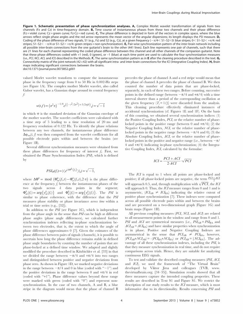
valued Morlet wavelet transform to compute the instantaneous
phase in the frequency range from 0 to 50 Hz in 0.002-Hz steps
(see Figure 1A). The complex mother Morlet wavelet, also called
Gabor wavelet, has a Gaussian shape around its central frequency
f:
w(t,f )~ s2p� �{1=4
e {t2=2s2ð Þz3=2pjftð Þ,j~ffiffiffiffiffiffiffiffi{1p
in which s is the standard deviation of the Gaussian envelope of
the mother wavelet. The wavelet coefficients were calculated with
a time step of 5 leading to a time resolution of 20 ms and
frequency resolution of 0.122 Hz. To identify the phase relations
between any two channels, the instantaneous phase difference
DQmn(t, f) was then computed from the wavelet coefficients for all
possible electrode pairs within and between the brains (see
Figure 1B).
Several different synchronization measures were obtained from
these phase differences for frequency of interest fi. First, we
obtained the Phase Synchronization Index (PSI), which is defined
by
PSIW(fi)~DSejDWk fið ÞTD,j~ffiffiffiffiffiffiffiffi{1p
,
where DWk~ mod Wkm fi,tð Þ{Wk
n fi,tð Þ,2:p� �
is the phase differ-
ence at the frequency fi between the instantaneous phases of the
two signals across k data points in the segment;
Wkm fið Þ~ arg yk
m fið Þ� �
and Wkn fið Þ~ arg yk
n fið Þ� �
. The PSI is
similar to phase coherence, with the difference that the PSI
measures phase stability or phase invariance across time within a
trial or time series (e.g., [32]).
In addition to the PSI (see Figure 1C), which is independent
from the phase angle in the sense that PSI can be high at different
phase angles (phase angle differences), we calculated further
synchronization indexes reflecting in-phase synchronization be-
tween two electrodes, that is, the extent to which the angle of
phase differences approximates 0 [7]. Given the estimates of the
phase difference between pairs of signals (channels), it is possible to
ascertain how long the phase difference remains stable in defined
phase angle boundaries by counting the number of points that are
phase-locked at a defined time window. We adapted and slightly
modified the procedure described in Kitzbichler et al. [33] in that
we divided the range between 2p/4 and +p/4 into two ranges
and distinguished between positive and negative deviations from
phase zero. As shown in Figure 1D, we marked negative deviations
in the range between 2p/4 and 0 in blue (coded with ‘‘21’’) and
the positive deviations in the range between 0 and +p/4 in red
(coded with ‘‘+1’’). Phase difference values beyond these range
were marked with green (coded with ‘‘0’’) and represent non-
synchronization. In the case of two channels, A and B, a blue
stripe in the diagram would mean that the phase of channel B
precedes the phase of channel A and a red stripe would mean that
the phase of channel A precedes the phase of channel B. We then
counted the number of data points that are phase-locked,
separately, in each of these two ranges. Before counting, successive
points in the defined range (between 2p/4 and +p/4) with a time
interval shorter than a period of the corresponding oscillation at
the given frequency (Ti = 1/fi) were discarded from the analysis.
This cleaning procedure effectively eliminated instances of
accidental synchronization (cf. Figures 1E and 1F). On the basis
of this counting, we obtained several synchronization indices: (1)
the Positive Coupling Index, PCI, or the relative number of phase-
locked points in the positive range (between 0 and +p/4); (2) the
Negative Coupling Index, NCI, or the relative number of phase-
locked points in the negative range (between 2p/4 and 0); (3) the
Absolute Coupling Index, ACI, or the relative number of phase-
locked points in the positive and negative range (i.e., between 2p/
4 and +p/4) indicating in-phase synchronization; (4) the Integra-
tive Coupling Index, ICI, calculated by the formulae:
ICI~PCIzACI
2:ACI:ffiffiffiffiffiffiffiffiffiPCIp
The ICI is equal to 1 when all points are phase-locked and
positive; if all phase-locked points are negative, the term PCIzACI2
will approach 0.5, and, through multiplication withffiffiffiffiffiffiffiffiffiPCIp
, the ICI
will approach 0. Thus, the ICI measure ranges from 0 and 1 and is
asymmetric, (ICIAB ? ICIBA) indicating the relative extent of
positive phase synchronization [7]. These indexes were computed
across all possible electrode pairs within and between the brains
and are presented on a two-dimensional graph (Figure 1G) and
brain maps (Figure 1H).
All previous coupling measures (PCI, NCI, and ACI) are related
to all measurement points in the window and range from 0 and 1.
PSI and ACI are symmetrical measures (i.e., PSIAB = PSIBA and
ACIAB = ACIBA) and have similar properties when synchronization
is in phase. Positive and Negative Coupling Indexes are
asymmetrical in the sense that PCIAB ? PCIBA, however,
(PCIAB+NCIAB) = –(PCIBA+NCIBA) or PCIAB = |NCIBA|. The ad-
vantage of all these synchronization indexes, including the PSI, is
that they measure synchronization in real time, and do not require
comparisons across trials. Hence, they are suitable for analyzing
continuous EEG signals.
To test and validate the described coupling measures (PSI, ACI,
and ICI), we used the framework of ‘‘The Virtual Brain’’
developed by Viktor Jirsa and colleagues (TVB, www.
thevirtualbrain.org; [34–35]). Simulation results showed that all
three measures capture the intended coupling properties. These
results are described in Text S1 and Figure S1. We restrict the
description of our study results to the ICI measure, which is most
informative due to its directionality. Results concerning PSI and
Figure 1. Schematic presentation of phase synchronization analyses. A, Complex Morlet wavelet transformation of signals from twochannels (Fz and Cz) in time-frequency domain. B, Time course of instantaneous phases from these two channels and their phase difference(Fz = violet curve; Cz = green curve; Fz-Cz = red curve). C, The phase difference is depicted in form of the vectors in complex space, where the bluearrows reflect single phase angles and the red arrow represents the mean vector of the angular dispersions; its length displays the PSI measure. D,Coding of the phase difference of two signals, S1 (e.g., Fz) and S2 (e.g., Cz), at a given frequency (2p/4, S1–S2,0: blue stripes; 0, S1–S2, +p/4: redstripes; S1–S2, 2p/4 or S1–S2. +p/4: green stripes = non-synchronization). E, Pair-wise synchronization pattern of the inter-brain network includingall possible inter-brain connections from the one guitarist’s brain to the other (441 lines). Each line represents one pair of channels, such that thereare 21 lines for each channel representing the coded phase difference between this channel and all other channels of the companion guitarist. Notethat these phase differences coded with +1 (red), 0 (green), or –1 (blue) at each time point are used to calculate the four synchronization measures(i.e., PCI, NCI, ACI, and ICI) described in the Methods. F, The same synchronization pattern as in E after the cleaning procedure described in the text. G,Connectivity matrix of the joint network (42642) with all significant intra- and inter-brain connections for the ICI (Integrative Coupling Index). H, Brainmaps indicating significant connections between the brains.doi:10.1371/journal.pone.0073852.g001
Inter-Brain Couplings during Musical Improvisation
PLOS ONE | www.plosone.org 4 September 2013 | Volume 8 | Issue 9 | e73852
ACI can also be found in the Text S1 and corresponding
Supplementary Figures.
Graph-Theoretical Approach (GTA)Threshold determination. To determine the network
properties, the thresholds of the synchronization or coupling
measures were calculated first. For this purpose we generated
surrogate data through a random permutation of available data
points (‘‘shuffling’’) of all epochs at all channels included in the
analyses, and then calculated the corresponding synchronization
measures between all possible electrode pairs on the basis of these
surrogate data. Thereafter, we applied a bootstrapping procedure
with 1,000 resamples of the coupling measures obtained from the
surrogate data set and determined the threshold as the boot-
strapping mean plus the confidence interval at a significance level
of p,0.0001 [36–38]. We used a high threshold level to obtain
sparse networks with highly reliable connections. Only coupling
values larger than the threshold value were considered as a link or
edge in the given network.
Degrees and strengths. As ICI is a directed measure, we
obtained the degree as the sum of in- and out-degrees, in which
the in-degree is the sum of all incoming connections, kini ~
Pj[N
aji,
and the out-degree is the sum of all outgoing connections,
kouti ~
Pj[N
aij . To calculate strengths, we then replaced the sum of
the links with the sum of weights, kwi ~
Pj[N
wij . Thus, the strength
can be considered as the weighted degree [20]. We determined
degrees and strengths for the whole network of each guitarist pair
and then calculated them for the within-brain network of each
guitarist (A and B) separately. To exclusively determine the
between-brain degrees and strengths, we subtracted degrees (and
respectively strengths) of the within-brain network from the
corresponding links of the network including both brains.
Clustering Coefficient (CC) and Characteristic Path
Length (CPL). If the nearest neighbors of a node are also
directly connected to each other, they form a cluster. For an
individual node, the CC is defined as the proportion of the existing
number of connections to the total number of possible connec-
tions:
Ci~2ti
ki(ki{1)or Cw
i ~2tw
i
ki(ki{1)
for binary and weighted networks, respectively, with
ti~12
Pj,h[N
aijaihajhbeing the number of triangles around a node i.
Usually, Ci is averaged over all nodes to obtain a mean clustering
coefficient (CC) of the graph:
CC~1
n
Xi[N
Ci:
In the case of a directed graph, the mean CC is calculated by the
formula:
CC~1
n
Xi[N
Cdi ~
1
n
Xi[N
tdi
(kouti zkout
i )(kouti zkout
i {1){2Pj[N
aijaji
:
Random networks have low average clustering coefficients,
whereas complex or small-world networks have high clustering
coefficients (associated with high local efficiency of information
transfer and robustness). Thus, the clustering coefficient is a
measure of segregation.
Another important measure is the CLP. In the case of an
unweighted graph, the shortest path length or distance di,j between
two nodes i and j is the minimal number of edges that have to be
passed to go from i to j. This is also called the geodesic path
between the nodes i and j. The CLP of a graph is the mean of the
path lengths between all possible pairs of vertices:
CPL~1
n
Xi[N
Li~1
n
Xi[N
Pj[N,j=i dij
n{1:
In the case of a weighted and directed graph the weight and
direction of the links will be considered.
Random and complex real networks (or small-world networks,
SWNs) have a short CPL (high global efficiency of parallel
information transfer), whereas regular lattices have a long CPL. In
this sense, CPL shows the degree of network integration, with a
short CPL indicating higher network integration.
Small-worldness coefficients. To investigate the small-
world properties of a network, it is common practice to compare
its clustering coefficient and characteristic path length to those of
regular lattices and random graphs. For this purpose, we
constructed regular (lattice) and random networks that have the
same number of nodes and the same mean degree as the observed
networks. Random networks were constructed through random-
ization of the edges in the observed network. Lattice networks
were configured like random networks, but edges were addition-
ally redistributed after an initial random permutation such that
they lie close to the main diagonal [39]. These network
reconstructions for random and regular networks were carried
out 20 times for each individual network. Average CC and CPL
were then determined for these individual control networks.
Using these graph metrics, specific quantitative small-world
metrics were obtained. The first small-world metric, the so-called
small-world coefficient s, is related to the main metrics of a
random graph (CCrand and CPLrand) and is determined on the basis
of two ratios c~CC=CCrand and l~CPL=CPLrand :
s~c
l~
CC=CCrand
CPL=CPLrand
The small-world coefficient s has been used in numerous
networks showing small-world properties and has been found to be
greater than 1 in the SWN (s .1). The second small-world metric,
the so-called small-world coefficient v, is defined by comparing
the clustering coefficient of the observed network to that of an
equivalent lattice network and comparing the characteristic path
length of the observed network to that of an equivalent random
network:
v~CPLrand
CPL{
CC
CClatt
This metric is ranged between 21 and +1 and is close to zero
for SWN (CPLSWN<CPLrand and CCSWN<CClatt). Thereby,
negative values indicate a graph with more regular properties
Inter-Brain Couplings during Musical Improvisation
PLOS ONE | www.plosone.org 5 September 2013 | Volume 8 | Issue 9 | e73852

(CPLSWN..CPLrand and CCSWN<CClatt), and positive values of vindicate a graph with more random properties (CPLSWN<CPLrand
and CCSWN,,CClatt ). The clear advantage of the metric vcompared to s is the possibility to define how much the network of
interest is like its regular or random equivalents [40].
Community structures and definition of node roles within
the brain networks. To further investigate the topological
properties of the hyper-brain networks, community structures for
weighted undirected and directed networks, as well as indices of
modularity (M), the within-module degree (Zi) and the participa-
tion coefficient (Pi) were determined (cf. [20]). For this calculation,
the modularity optimization methods [41,42] were used, which are
implemented in the Brain Connectivity Toolbox (https://sites.
google.com/site/bctnet/; cf. [20]). The optimal community
structure is a subdivision of the network into non-overlapping
groups of nodes in a way that maximizes the number of within-
module edges, and minimizes the number of between-module
edges. The modularity (M) is a statistic that quantifies the degree to
which the network may be subdivided into such clearly delineated
groups or modules and is given for weighted networks by the
formula [42]:
Mw~1
lw
Xi,j[N
wij{kw
i kwj
lw
� �:dmi ,mj ,
where lw~P
ij wij and wij represents the weight of the edge
between i and j, N is the total number of nodes in the network, kwi
and kwj are weighted degrees or strengths of the nodes i and j, mi is
the module containing node i, mj is the module containing node j,
and dmi ,mjis the Kronecker delta, where dmi ,mj
= 1 if mi = mj, and 0
otherwise. For directed unweighted networks, modularity was
calculated in similar way by the formula [41]:
M?~1
l
Xi,j[N
aij{kin
i kouti
l
� �:dmi ,mj ,
where l~P
ij aij is the number of edges in the graph, and aij is
defined to be 1 if there is an edge from j to i and zero otherwise, kini
and kouti are the in- and out-degrees of the node i, and dmi ,mj
is
again the Kronecker delta. High modularity values indicate strong
separation of the nodes into modules. M = 0 if nodes are placed at
random into modules or if all nodes are in the same cluster [43].
The within-module degree Zi indicates how well node i is
connected to other nodes within the module mi. It is determined
by
Zi~ki(mi){�kk(mi)
sk(mi ),
where ki(mi) is the within-module degree of node i (the number of
links between i and all other nodes in mi). �kk(mi) and sk(mi ) are the
mean and standard deviation of the within-module degree
distribution of mi. The within-module degree Zi is 0 if all the
nodes of the module have the same number of edges (e.g., if all the
nodes within the module are fully interconnected with each other);
otherwise, it has negative or positive values depending on the
number of links at the different nodes.
The participation coefficient Pi describes how well the nodal
connections are distributed across different modules:
Pi~1{Xm[M
ki(mi)
ki
2
,
M is the set of modules, ki(mi) is the number of links between
node i and all other nodes in module mi, and ki is the total degree
of node i in the network. Correspondingly, Pi of a node i is close to
1 if its links are uniformly distributed among all the modules and 0
if all of its links lie within its own module. Zi- and Pi-values are
characteristic for the different roles of the nodes in the network
[43].
Following Guimera and Amaral [43], we heuristically defined
eight different universal roles, each characterized by Z- and P-
values dividing the Z-P parameter space into eight different
regions:
R1 (Z,1.4; P,0.05) – non-hub ultra-peripheral nodes,
R2 (Z,1.4; 0.05,P,0.5) – non-hub peripheral nodes,
R3 (Z,1.4; 0.5,P,0.8) – non-hub connector nodes,
R4 (Z,1.4; P.0.8) – non-hub kinless nodes,
R5 (Z.1.4; P,0.05) – hub ultra-peripheral nodes,
R6 (Z.1.4; 0.05,P,0.5) – hub peripheral nodes,
R7 (Z.1.4; 0.5,P,0.8) – hub connector nodes,
R8 (Z.1.4; P.0.8) – hub kinless nodes.
The community structures and corresponding measures (M, Zi,
and Pi) were determined for the joint networks of the two guitarists
and for each individual brain separately. As the separate within-
brain networks showed relatively low modularity values (M ,0.30;
cf. [44,45]), we only report results for the joint networks. All GTA
measures described here were determined using the Brain
Connectivity Toolbox (cf. [20]) for 17 frequency components: 2,
3, 4, 5, 6, 7, 8, 9, 10, 11, 12, 14, 16, 18, 20, 24, and 28 Hz.
EEG Data Reduction and Statistical AnalysesFor statistical analyses, we collapsed frequencies into five bands:
delta (2–3 Hz), theta (4–7 Hz), alpha (8–12 Hz), beta1 (14–20 Hz)
and beta2 (24–28 Hz). Also, individual electrodes were collapsed
into three regions along the anterior-posterior axis (frontal, central
and parieto-occipital). Degrees and strengths were statistically
evaluated for hyper-brain networks and separately for within- and
between-brains connections. A four-way repeated-measures AN-
OVA with a between-subject factor Guitarist (guitarist A vs.
guitarist B) and three within-subject factors Play Condition (Play
A, Play B, and Play AB), Frequency Band (delta, theta, alpha,
beta1, and beta2), and Site (frontal, central, and parietal) was used
for all the coupling measures (PSI, ACI, and ICI). CC, CPL, and M,
which were determined for hyper-brain networks only, were tested
using a two-way repeated-measures ANOVA with two within-
subject factors Play Condition and Frequency Band.
Results
By simultaneously recording the EEG of two people, we
measured the electrophysiological brain activity of eight pairs of
guitarists during musical improvisation. The two guitarists were
either playing simultaneously, or one of them was playing while
the other was listening. A video recording of a pair of guitarists
playing together with the corresponding EEG is available as a
Movie S1. As mentioned in the Methods section, we restrict the
description of our results to the directed ICI measure. Results
regarding PSI and ACI can be found in the Supporting
Information files. With a few exceptions, the pattern of results
Inter-Brain Couplings during Musical Improvisation
PLOS ONE | www.plosone.org 6 September 2013 | Volume 8 | Issue 9 | e73852

obtained with PSI and ACI matched the pattern of results obtained
with ICI.
Phase Synchronization and Brain Connectivity PatternsIn Figure 2, we illustrate time-frequency diagrams of synchro-
nization patterns between two electrodes within (Fza to Pza or Fzb
to Pzb; see Figure 2A and 2B, respectively) and between (Fza to
Fzb and Pza to Pzb, see Figure 2C and 2D, respectively) the brains
in the frequency range between 0 and 30 Hz while (i) guitarist A is
playing and guitarist B is listening; (ii) guitarist B is playing and
guitarist A is listening; and (iii) both guitarists are playing together.
It can be seen that in all these cases there is a complex interplay of
synchronization patterns across frequencies and time, with the
direction of temporal phase differences marked in blue and red,
respectively. It is not surprising that synchronization within the
brains is always stronger than that between the brains, but
synchronization both within and between the brains seems to be
strongly related to the plucked notes or chords that are played
(compare Figure 2E). Furthermore, there is strong phase
alignment across frequencies, which indicates coactivity between
different networks operating in different frequency domains.
Within-brains synchronization patterns at the frequency of
interest (fi = 6 Hz) across all possible electrode pairs for guitarists A
and B are presented in Figures 3A and 3B, respectively. The
between-brains synchronization pattern is depicted in Figure 3C.
Corresponding recordings of acoustic channels for guitarists A and
B as well as the AB duet are presented below in the respective
synchronization patterns in Figure 3D. The connectivity matrices
corresponding to the individual and duet synchronization patterns
can be found in Figure 3E. The brain maps for ICI within and
between the brains are presented in Figures 3F (within) and 3G
(between). All panels in Figure 3 represent three playing conditions
(Play A, Play B, and Play AB). For better visualization, brain maps
containing the strongest within- and between-brain connections
are depicted. Figure S2 shows the entire network with all
significant connections within and between the brains.
Intra-brain connections were distributed across the entire cortex
involving different brain regions or networks (prefrontal, motor,
auditory, visual cortices, etc.) in both the playing and the listening
guitarist, with slightly stronger interconnectivity within the playing
guitarist’s brain. The inter-brain connectivity differed between the
two guitarists: While guitarist A showed strong outgoing connec-
tions from frontal and central regions, the outgoing connections of
guitarist B are distributed across different regions, with a relatively
high number of connections going to frontal and occipital (e.g.,
Oz) electrodes of guitarist A. However, it should be noted here
that connectivity patterns varied from pair to pair and across
segments within pairs. To describe these changes in greater detail,
we used the GTA.
Statistical Evaluation of GTA MeasuresDegrees and strengths. Strengths averaged across partici-
pants separately for the three play conditions and 21 electrode sites
are represented in Figure S3 for some frequencies of interest (6, 10,
16 and 28 Hz). At higher frequencies (8 Hz and higher), strengths
(in- and out-strengths) of the playing guitarists within their brains
were higher than that of listening guitarists. This is particularly the
case when playing solo. In addition, there were low strengths
between the brains in the duet-playing condition in the alpha
frequency range (e.g., 10 Hz), and high strengths between the
brains in the beta1 frequency range, especially at 16 Hz.
For statistical analyses, we collapsed frequencies into five bands:
delta (2–3 Hz), theta (4–7 Hz), alpha (8–12 Hz), beta1 (14–20 Hz)
and beta2 (24–28 Hz). Also, individual electrodes were collapsed
into three regions along the anterior-posterior axis (frontal, central
and parieto-occipital). We obtained relatively similar results for
degrees and strengths as well as in- and out-degrees/2strengths.
Therefore, we only present out-strengths here, which are more
informative than degrees since they account for the weights of the
network links. The out-strengths were determined for the whole
network of the duet, encompassing both within- and between-
brain connections as well as separately for within- and between-
brain networks. For the joint networks, a four-way repeated-
measures ANOVA (Guitarist6Play Condition6Frequency Band
6 Site) for ICI revealed significant main effects of Frequency
Band, F(4,56) = 28.2, P,0.0001, g2 = 0.67, and Site,
F(2,28) = 28.0, P,0.0001, g2 = 0.67, indicating an increase in
strengths with higher frequency and a decrease in strengths from
frontal to parieto-occipital regions. Furthermore, significant
interactions of Guitarist 6 Play Condition, F(2,28) = 4.0,
P,0.05, g2 = 0.22, and Guitarist 6Play Condition 6Frequency
Band, F(8,112) = 10.1, P,0.0001, g2 = 0.42, were found, indicat-
ing higher strengths in the playing guitarist compared to his or her
listening partner. This difference was especially pronounced for
both beta frequency bands (i.e., beta1 and beta2). When both
guitarists were playing, there were no significant differences
between them. Similar results were found for within-brain
networks: Frequency Band, F(4,56) = 67.8, P,0.0001, g2 = 0.83;
Site, F(2,28) = 24.4, P,0.0001, g2 = 0.64; Guitarist 6 Play
Condition, F(2,28) = 4.1, P,0.05, g2 = 0.23; Guitarist 6 Play
Condition 6 Frequency Band, F(8,112) = 11.4, P,0.0001,
g2 = 0.45. In the between-brain network, however, statistical
analyses of strengths showed a significant decrease of strengths
with increasing frequency, indicated by the significant main effect
Frequency Band, F(4,56) = 216.0, P,0.0001, g2 = 0.94, and the
significant Frequency Band 6 Play Condition interaction,
F(8,112) = 3.0, P,0.05, g2 = 0.18. This inverse relationship
reflected variations in both within- and between-brains connec-
tions: increasing strength with higher frequency within the brains,
and decreasing strength with higher frequency between the brains
(see Table 1).
Clustering Coefficient (CC) and Characteristic Path
Length (CPL). CC and CPL were determined across all pairs
of guitarists for different frequency bins and play conditions, taking
into account intra- and inter-brain connections. Particular
frequencies were then collapsed into the five frequency bands
and analyzed using two-way repeated measures ANOVA (Play
Condition 6Frequency Band).
The rmANOVA showed a significant main effect of Frequency
Band only, indicating significant changes across the frequency
bands: CC increased with higher frequencies, F(4,28) = 158.8,
P,0.0001, g2 = 0.96), and CPL decreased, at least for beta1 und
beta2 frequency bands, F(4,28) = 29.6, P,0.0001, g2 = 0.81.
Small-worldness of hyper-brain networks. The small-
world characteristics (s and v) for the ICI measure in the different
frequency bands averaged across the three play conditions and all
guitarist pairs are presented in Figure 4. According to the small-
world coefficient s, the ICI-based hyper-brain networks corre-
spond to the SWN, wherein s is always greater than 1 and
increases with higher frequency. The small-world coefficient vdecreases with higher frequency and ranges between –0.22 and
0.05. This indicates that networks based on ICI possess more
random characteristics for the delta frequency band and more
regular characteristics for the beta frequency band. Statistical
analysis revealed only a significant main effect of Frequency Band
for both coefficients (s and v): s, F(4,28) = 46.38, P,0.0001,
g2 = 0.87), and v, F(4,28) = 72.08, P,0.0001, g2 = 0.91).
Inter-Brain Couplings during Musical Improvisation
PLOS ONE | www.plosone.org 7 September 2013 | Volume 8 | Issue 9 | e73852

Modularity, community structures and the Z-P
parameter space. Modularity (M), which was analyzed in the
same way as CC and CPL, showed a significant increase with
frequency, F(4,28) = 178.1, P,0.0001, g2 = 0.96, indicating the
stronger partitioning of networks synchronizing or communicating
at high frequencies (e.g., beta frequency bands).
To define how nodes were positioned in their own module and
with respect to other modules, we calculated the within-module
Figure 2. Phase synchronization patterns across frequencies (0–30 Hz) of one pair of guitarists under the three playing conditions(Play A, Play B, and Play AB). A, Phase synchronization patterns within the brain of guitarist A (Fza to Pza). B, Phase synchronization patternswithin the brain of guitarist B (Fzb to Pzb). C, Phase synchronization patterns between the brains at the frontal electrode sites (Fza to Fzb). D, Phasesynchronization patterns between the brains at the parietal electrode sites (Pza to Pzb). E, Microphone traces of guitar A (yellow) B (purple),respectively. Play A: Guitarist A is playing and guitarist B is listening; Play B: Guitarist B is playing and guitarist A is listening; Play AB: Both guitarist Aand B are playing.doi:10.1371/journal.pone.0073852.g002
Inter-Brain Couplings during Musical Improvisation
PLOS ONE | www.plosone.org 8 September 2013 | Volume 8 | Issue 9 | e73852

Inter-Brain Couplings during Musical Improvisation
PLOS ONE | www.plosone.org 9 September 2013 | Volume 8 | Issue 9 | e73852

degree (Zi) and participation coefficient (Pi) of the node i for the
whole network of a given pair. The within-module degree
measures how ‘well-connected’ node i is to other nodes in the
module, whereas the participation coefficient reflects how ‘well-
distributed’ the links of the node i are among the other modules. Zi
and Pi form together the so-called Z-P parameter space, with
different regions indicating specific roles of the nodes in this space
or these regions.
Figure 5 displays community structures and Z-P parameter
spaces for the three play conditions (Play A, Play B, and Play AB)
for all pairs of guitarists across the 10 different trials (see
Figures 5A, 5B, and 5C). When comparing community structures
at different frequencies (see Figure S4), we noticed that (i) the
brains of the two guitarists being in different musical roles can
always be differentiated independently of the frequency and the
number of modules, (ii) the number of modules decreased with
increasing frequency from about 3–4 (sometimes 5) in the delta
and theta band to about 2–3 modules in the beta2 band, and (iii)
there were cases at all frequencies in which some electrodes from
different brains shared the same module (see Figures 5D and 5E).
Regarding the Z-P parameter space, we noticed for all the
measures a clear separation at P = 0.5 dividing the Z-P space into
two regions: peripheral nodes (P#0.5) and connectors (P.0.5).
According to the within-module degree, nodes with Z $1.4 were
defined as hubs and nodes with Z ,1.4 were defined as non-hubs.
This separation Z-value was chosen arbitrarily but it corresponds
to the definition of hubs as nodes containing much more edges
than the most of the nodes in the module (cf. [43]). The number of
hubs varied between 0.6% and 2.8% for all the three measures at
different frequencies. Depending on the participation coefficient,
we further divided hubs and non-hubs into eight different roles:
(R1) ultra-peripheral non-hubs (P#0.05), (R2) peripheral non-
hubs (0.05,P#0.5), (R3) connector non-hubs (0.5,P#0.8), (R4)
kinless non-hubs (0.8,P#1.0), and R5–R8 are then ultra-
peripheral, peripheral, connector, and kinless hubs, respectively.
We calculated the number of nodes falling into these regions.
Results of this calculation for the ICI at different frequencies are
displayed in Figure 6. It can be seen that the number of peripheral
nodes, especially of ultra-peripheral nodes, increased with higher
frequency, whereas the number of connectors decreased. These
tendencies apply to both hubs and non-hubs. Interestingly, the low
number of peripheral nodes was compensated by the high number
of ultra-peripheral nodes, and vice versa (e.g., at the beta
frequency 14–28 Hz). Furthermore, there was a higher number
of non-hub connectors during separate playing (Play A and Play B)
than during joint playing (Play AB) at the alpha frequency (8–
12 Hz), whereas the joint playing was accompanied by a higher
number of hub-connectors at the delta (2–3 Hz) and theta (5–
7 Hz) frequency. We note that the present observations of
differences between joint and separate playing are not backed
up by inference statistics but are descriptive, and hence should be
treated with caution. Please note that results regarding ACI and
PSI measures are presented in Text S1, Tables S1 and S2, and
Figures S5, S6, S7, and S8.
Discussion
The primary objective of this study was to investigate the intra-
and inter-brain dynamics in pairs of guitarists improvising
together. In contrast to our previous studies [4,6], where phase
synchronization was measured across trials, we were interested in
obtaining phase synchronization indices that can be applied to
continuous data, or single trial analyses. Hence, we established
directed and undirected synchronization or coupling measures
derived from instantaneous changes in phase synchronization or
phase differences between two EEG signals across time at different
frequencies. These coupling indices measure different aspects of
phase synchronization and are suitable for single-trial analysis (see
also Text S1).
We observed phase synchronization patterns in the time-
frequency domain and showed that intra- and inter-brain phase
synchronization were operating at overlapping frequencies with
different modes, such that the phase of a given signal at a given
frequency can precede or follow another signal in phase.
Generally, however, phase alignment across frequencies was a
prominent feature of the data. Frequencies aligned in phase
support the hypothesis that cell assemblies both within and
between the brains synchronize during activities that require
Figure 3. Phase synchronization patterns at the frequency of interest (6 Hz) for all possible electrode pairs within and between thebrains under the three play conditions (Play A, Play B, and Play AB). A, Phase synchronization patterns within the brain of guitarist A. B,Phase synchronization patterns within the brain of guitarist B. C, Phase synchronization patterns between the brains of the guitarists A and B. D,Microphone traces of guitar A (yellow) and B (purple), respectively. E, Connectivity matrices of the joint network (42642) with all significant intra- andinter-brain connections for the ICI (Integrative Coupling Index). F, Brain maps indicating significant connections within the brains. G, Brain mapsindicating significant connections between the brains.doi:10.1371/journal.pone.0073852.g003
Table 1. Mean and standard deviation for strength of ICImeasures calculated separately for intra- and inter-brainconnections in the five frequency bands.
Frequency bands Intra-brain Inter-brain
Delta 7.42 (1.21) 2.28 (0.11)
Theta 8.05 (1.33) 1.86 (0.16)
Alpha 8.22 (1.50) 1.40 (0.13)
Beta 1 9.25 (1.39) 1.15 (0.09)
Beta 2 10.24 (1.43) 1.18 (0.14)
doi:10.1371/journal.pone.0073852.t001
Figure 4. Small-worldness coefficients sigma (s) and omega (v)for the ICI measure in the five frequency bands (delta, theta,alpha, beta 1,and beta 2). The X-axis corresponds to the fivefrequency bands: De = Delta, Th = Theta, Al = Alpha, Be1 = Beta 1, andBe2 = Beta 2.doi:10.1371/journal.pone.0073852.g004
Inter-Brain Couplings during Musical Improvisation
PLOS ONE | www.plosone.org 10 September 2013 | Volume 8 | Issue 9 | e73852

Inter-Brain Couplings during Musical Improvisation
PLOS ONE | www.plosone.org 11 September 2013 | Volume 8 | Issue 9 | e73852

interpersonal action coordination in the time domain, such as
musical improvisation. Phase-specific differences in phase state
may suggest that the putative causal influence from one signal to
the other is frequency dependent and may go in different
directions at the same time.
Graph-theoretical Measures: Degrees and StrengthsNext, we used graph-theoretical measures to describe the
properties of intra- and inter-brain networks while improvising on
the guitar in pairs. We found that (i) the strengths of outgoing
connections increased with higher frequencies and were strongest
at frontal sites, irrespective of the frequency, and (ii) the guitarist
playing alone showed higher out-strengths than the listening
guitarist, especially at the beta1 and beta2 frequencies, while no
significant differences (between the two guitarists) were found
when both guitarists were playing. Another interesting result was
that strengths decreased with frequency in the between-brain
networks, but increased with frequency in the within-brain
networks. This inverse association suggests that intra-brain and
inter-brain synchronization are operating at different modal
frequencies.
In the study of Dumas et al. [3], three different inter-brain
synchronization clusters among alpha-mu, beta and gamma
frequency bands were found during spontaneous imitation
episodes. In accordance with our findings, inter-brain synchroni-
zation measured by Phase Locking Value (PLV, a measure like PSI
in our study) was higher in the alpha-mu frequency band than in
the beta and gamma frequency bands. Furthermore, inter-brain
synchronization comparing induced imitation episodes with ‘‘No
View Motion’’ baseline could be found in the theta band only. The
present results also replicate our earlier work, where inter-brain
synchronization in guitarist duets as measured by Inter-Brain
Phase Coherence (IPC) was predominantly observed in the delta
and theta frequency bands [4,6]. Taken together, the findings
suggest a preponderance of low frequencies in inter-brain
synchronization. Using the directed ICI measure, which reflects
both strength and earliness in the phase angle, we were able to
further specify this observation in the present study.
As indicated by a Frequency Band6Play Condition interaction
for the inter-brain strengths, solo playing was accompanied by
higher strengths in the alpha frequency range, while joint playing
requires higher strengths in the beta1 frequency range (e.g., 16 Hz
as shown in Figure S3). Joint playing is more of an interaction than
solo playing and requires fast action coordination, which may be
supported by faster frequencies. We have shown that inter-brain
coupling generally prefers lower frequencies but faster frequencies
may sometimes be required to support highly coordinative actions.
Small-worldness, Segregation and Integration of Hyper-brain Networks
As a graph theory description of brain networks, we also
computed the CC and the CPL as measures of segregation and
integration, respectively [20,46,47]. We found that both the CC
and CPL of the joint network of the two guitarists’ brains were
frequency dependent. Whereas the CC increased with higher
frequency, CPL decreased. Thus, directed networks measured by
ICI showed stronger segregation and stronger integration at higher
frequencies (e.g., beta1 and beta2). This tendency generalized
across the two playing conditions.
To investigate the small-world properties of the hyper-brain
networks, we compared their CC and CPL to those of regular
lattices and random graphs. In general, random networks have a
low average clustering coefficient, whereas complex or small-world
networks have a high clustering coefficient (associated with the
high local efficiency of information transfer and robustness).
Random and small-world networks have a short CPL (high global
efficiency of parallel information transfer), whereas regular
networks (e.g., lattices) have a long CPL. To investigate small-
world properties of the guitarists hyper-brain networks, we
constructed regular and random networks with the same number
of nodes and mean degree as our real networks and calculated two
different small-worldness coefficients (i.e., s and v). According to
the small-world coefficient s, the directed hyper-brain networks
correspond to SWN, whereby s increases with higher frequency.
This increase of s for ICI with higher frequency corresponds to
the increase of CC and decrease of CPL mentioned above. The fact
that the small-worldness coefficient v decreases with higher
frequency and goes from positive (e.g., delta frequency band) to
negative (especially for beta frequency band) indicates that ICI-
based hyper-brain networks become more regular at higher
frequencies. This seems to be a general tendency of the hyper-
brain networks, because their small-world coefficients did not vary
as a function of the play condition. In an MEG study, Stam [48]
showed that binary unweighted networks correspond to SWNs for
the delta and theta frequency bands, but are regular for the alpha
and beta frequency bands. In an EEG study [49], where SWN
properties were investigated using the synchronization measure at
different frequencies, a decrease of small-worldness with higher
frequency was also shown. The small-world index was not
calculated by the authors, but can be obtained from changes in
relative CC (c) and CPL (l); it approaches 1 at high frequencies.
Other studies also have reported changes in network topology with
a shift to more regular or more random networks, dependent on
frequency or frequency bands [50–53]. There is also neuro-
physiological evidence that small-world characteristics (e.g., CC
and CPL or c and l) can vary as a function of age [47,54,55] or
neuropathology [49,51,56–61], with a shift to a more regular or
more random network topology (for a review, see [62] as well as
[63]). According to a recent report, reduction in small-worldness is
associated with a decrease in local efficiency and with an abnormal
rise in interhemispheric connectivity [64]. Nevertheless, despite
the currently available data on variations in small-worldness, our
understanding of these differences is incomplete (see also results
regarding PSI and ACI measures in Text S1). Also, it needs to be
kept in mind that the results mentioned above all refer to single-
brain studies (cf. [65]). Thus, even less is known regarding inter-
brains networks. Further systematic research is needed to provide
better understanding of this very important issue.
Modular Properties of the Guitarists’ NetworksModularity (M) measured for joint networks revealed a
significant increase with higher frequencies, indicating a stronger
Figure 5. Community structures and distribution of nodes in a Z-P parameter space under the three play conditions (Play A, Play B,and Play AB). A–C, Community structure and Z-P parameter space for Play A, Play B and Play AB conditions. Community structure: In the X-axis(Cases), 10 trials of each of the 8 guitarist pairs are displayed. In the Y-axis (Electrodes), 21 electrodes of each guitarist in the pair are displayed. Thecolor indicates the electrodes’ module affiliation. Z-P parameter space: The X- and Y-axes correspond to Partition coefficient (P) and Within-moduledegree (Z), respectively. Yellow circles display guitarist A, and red circles – guitarist B. D–E, A case in which some electrode sites from different brainsshare the same module, is displayed.doi:10.1371/journal.pone.0073852.g005
Inter-Brain Couplings during Musical Improvisation
PLOS ONE | www.plosone.org 12 September 2013 | Volume 8 | Issue 9 | e73852
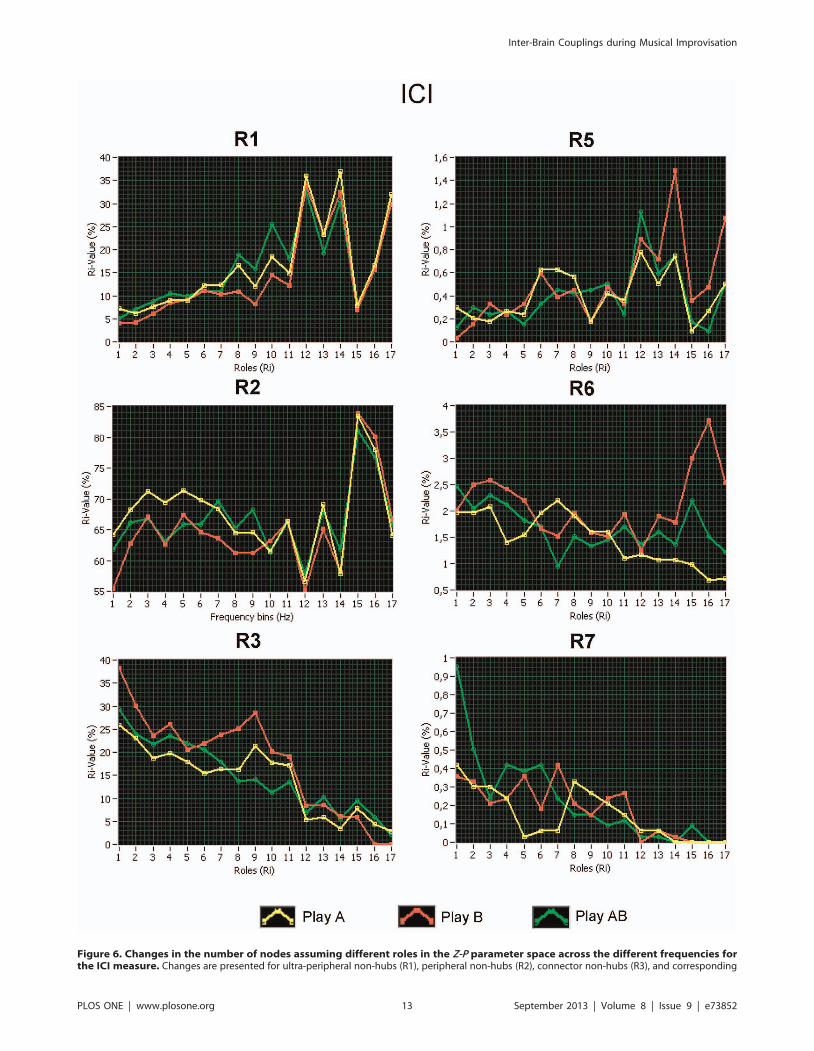
Figure 6. Changes in the number of nodes assuming different roles in the Z-P parameter space across the different frequencies forthe ICI measure. Changes are presented for ultra-peripheral non-hubs (R1), peripheral non-hubs (R2), connector non-hubs (R3), and corresponding
Inter-Brain Couplings during Musical Improvisation
PLOS ONE | www.plosone.org 13 September 2013 | Volume 8 | Issue 9 | e73852

partitioning of networks at higher frequencies. This stronger
partitioning was accompanied by a reduced number of modules,
with mostly two modules corresponding to the two brains of
guitarist A and B, respectively (e.g., at beta2 frequency). As
observed in our previous study [6], some nodes (electrode sites)
that comprised in the same module belonged to different brains.
The sharing of electrode sites from different brains in a common
module suggests that the brain areas under these electrodes may
participate in a function that engages both brains. Future research
needs to determine whether and in what way these brain areas
implement neuronal mechanisms of social interaction.
Next, we examined the Z-P parameter space of the joint
network by looking at the within-module degree (Z) and the
participation coefficient (P), which subdivide the Z-P parameter
space into the eight regions corresponding to eight different roles
of the nodes in the network: ultra-peripheral, peripheral,
connectors, and kinless hubs, and corresponding non-hubs. Non-
hub connectors are characterized by a low number of degrees or
strengths within the module, and by a relatively high number of
these between the modules. In contrast, hub-connectors have a
relatively a high number of degrees or strengths both within and
between the modules [43,66]. We calculated the number of nodes
assuming these different roles. A higher number of non-hub
connectors during solo playing (Play A and Play B) as compared to
joint playing (Play AB) could be found at the alpha frequency (8–
12 Hz), whereas the joint playing was accompanied by higher
number of hub-connectors at the delta (2–3 Hz) and theta (5–
7 Hz) frequency. Thus, coordinated guitar playing during jazz
improvisation increases the number of nodes having high
connectivity within and between the modules. In light of the
finding that strengths and degrees between brains increased at low
frequencies, we suggest that the increase of connector hubs at low
frequencies (e.g., delta and theta) during joint playing may be
related, at least in part, to between-brain connections. In sum, we
have shown that joint networks of guitarists’ duets during music/
jazz improvisation, derived from connectivity analyses using
different coupling measures, have a non-random modular
organization, where the nodes or electrode sites have different
functional roles within and between the modules, possibly
contributing to interpersonal action coordination (e.g., playing
guitar in duets).
Limitations and Issues for Future ResearchThe present study has limitations and leaves room for questions
to be addressed in future research. First, the sample size of our
study was small. Further studies with larger samples would provide
additional and more reliable information about coupling mech-
anisms during interpersonal action coordination. Second, certain
features of our data-analytic approach to the study of network
properties, such as the thresholding of coupling parameters and
the definition of topological roles in Z-P parameter space, are
somewhat arbitrary. Third, the synchronization measures used in
this study reflect 1:1 synchronization or synchronization at a given
frequency. Relative (i.e., n:m) as well as nonlinear (or weak)
synchronization [67,68] may also fulfill important functions during
interpersonal action coordination and should be investigated in the
future. Cross-frequency coupling between low and high frequen-
cies may be of particular importance, given that these frequencies
are differentially related to the coupling dynamics within and
between brains, as shown in the present study. Finally, and
perhaps most importantly, analyses of intra- and inter-brain
synchronization, such as the ones reported in this article, need to
be combined with detailed observations of the microstructure of
task-relevant behavior (e.g., gestures, eye movements) to better
understand how inter-brain synchronization is initiated and how
temporally specified expectations about the other person’s actions
are updated.
Conclusions
Extending a previous experimental design [4,6], we found that
within- and between-brain oscillatory couplings can also be
observed during musical improvisation on the guitar. Further-
more, these couplings were also present when one guitarist was
playing and the other was listening.
We found that synchronization patterns during guitar impro-
visation show a complex interplay of different frequencies. With
increasing frequencies, strengths increased in within-brain net-
works, but decreased in between-brain networks, suggesting that
intra-brain networks tend to operate at higher frequencies,
whereas inter-brain networks tend to operate at lower frequencies.
Furthermore, we found that the guitarist playing solo showed
higher out-strengths than the listening guitarist at higher
frequencies, while no significant differences (between the two
guitarists) were found when both guitarists were playing. Joint
playing was also accompanied by higher strengths in the beta1
frequency range, whereas solo playing was accompanied by higher
strengths in the alpha frequency range.
The inspection of community structures showed a higher
number of non-hub connectors during solo playing at the alpha
frequency (8–12 Hz), whereas the joint playing was accompanied
by a higher number of hub-connectors at the delta (2–3 Hz) and
theta (5–7 Hz) frequency. We also found that hyper-brain network
topology is frequency-dependent and approximates regular
networks with increasing frequency, independent of play condi-
tion. Finally, we identified modules composed of nodes from both
brains, so-called hyper-brain modules. The areas captured by
these nodes may point to brain regions that implement mecha-
nisms of interpersonal action coordination.
Supporting Information
Figure S1 Results of PSI, ACI, and ICI distributions forsimulated data at the three different frequencies. A–C,In this simulation, 5, 10, and 20 Hz oscillations with additive noise
were used. The oscillations were divided pairwise into epochs of
3,000 ms, thereby the second oscillation in the pair was randomly
shifted in phase, with a uniform distribution between –p and +p.
The coupling (PSI, ACI, and ICI) was determined for 10,000 such
epochs in total. Note that all three phase synchronization measures
capture the intended coupling properties (see text for details).
(TIF)
Figure S2 Network patterns and corresponding intra-and inter-brain maps at the frequency of interest (6 Hz)for the three coupling measures (PSI, ACI and ICI) underthe three play conditions. A, Connectivity matrices of the
joint network (42642) with all significant intra- and inter-brain
connections for the PSI (Phase Synchronization Index). B, Brain
maps indicating significant connections (PSI) within the brains. C,Brain maps indicating significant connections (PSI) between the
hubs (R5–R7) under the three conditions (Play A = yellow, Play B = red, and Play AB = green). Kinless hubs and non-hubs are excluded from thepresentation because the number of nodes assuming these roles was very low. X-axis: Frequency bins; Y-axis: Percentage of number of nodes.doi:10.1371/journal.pone.0073852.g006
Inter-Brain Couplings during Musical Improvisation
PLOS ONE | www.plosone.org 14 September 2013 | Volume 8 | Issue 9 | e73852
brains. D, Connectivity matrices of the joint network (42642) with
all significant intra- and inter-brain connections for the ACI
(Absolute Coupling Index). E, Brain maps indicating significant
connections (ACI) within the brains. F, Brain maps indicating
significant connections (ACI) between the brains. G, Connectivity
matrices of the joint network (42642) with all significant intra- and
inter-brain connections for the ICI (Absolute Coupling Index). H,Brain maps indicating significant connections (ICI) within the
brains. I, Brain maps indicating significant connections (ICI)
between the brains.
(TIF)
Figure S3 Out- and In-Strengths within and between thebrains separately for guitarist A and B at somefrequencies of interest (6, 10, 16 and 28 Hz) for the ICImeasure under the three play conditions (Play A, Play B,and Play AB). The X-axis represents 21 electrode (Fp1, Fpz,
Fp2, F7, …, O1, Oz, and O2) of each participant. The different
colours represent the play conditions: Play A = red, Play B = green,
and Play AB = blue.
(TIF)
Figure S4 Community structures for the ICI measure atsome frequencies of interest (2, 10, 16 and 28 Hz) underthe three play conditions (Play A, Play B, and Play AB). In
the X-axis (Cases), 10 trials of each of the 8 guitarist pairs are
displayed. In the Y-axis (Electrodes), 42 electrodes (21 of each
guitarist in the pair) are displayed. The color indicates the
electrodes’ module affiliation.
(TIF)
Figure S5 Strengths within and between the brainsseparately for guitarist A and B at some frequencies ofinterest (6, 10, 16 and 28 Hz) for the two undirectedmeasures PSI and ACI under the three play conditions(Play A, Play B, and Play AB). The X-axis represents 21
electrode (Fp1, Fpz, Fp2, F7, …, O1, Oz, and O2) of each
participant. The different colours represent the play conditions:
Play A = red, Play B = green, and Play AB = blue.
(TIF)
Figure S6 Small-worldness coefficients s and v for ACIand PSI measures in the five frequency bands (delta,theta, alpha, beta 1,and beta 2). A, Small-worldness
coefficients s and v for ACI. B, Small-worldness coefficients sand v for PSI. The X-axis corresponds to the five frequency bands:
De = Delta, Th = Theta, Al = Alpha, Be1 = Beta 1,and Be2 = Beta
2.
(TIF)
Figure S7 Changes in the number of nodes assumingdifferent roles in the Z-P parameter space across thedifferent frequencies for the PSI measure. Changes are
presented for ultra-peripheral non-hubs (R1), peripheral non-hubs
(R2), connector non-hubs (R3) and corresponding hubs (R5–R7)
under the three conditions (Play A = yellow, Play B = red, and Play
AB = green). Kinless hubs and non-hubs are excluded from the
presentation because the number of nodes assuming these roles
was very low. X-axis: Frequency bins; Y-axis: Percentage of
number of nodes.
(TIF)
Figure S8 Changes in the number of nodes assumingdifferent roles in the Z-P parameter space across thedifferent frequencies for the ACI measure. Changes are
presented for ultra-peripheral non-hubs (R1), peripheral non-hubs
(R2), connector non-hubs (R3) and corresponding hubs (R5–R7)
under the three conditions (Play A = yellow, Play B = red, and Play
AB = green). Kinless hubs and non-hubs are excluded from the
presentation because the number of nodes assuming these roles
was very low. X-axis: Frequency bins; Y-axis: Percentage of
number of nodes.
(TIF)
Table S1 Mean and standard deviation for strength of ACI and
PSI measures calculated separately for intra- and inter-brain
connections in the five frequency bands.
(DOCX)
Table S2 ANOVA results (F, P, and g2 values) for strength of
ACI and PSI measures calculated for hyperbrain, intrabrain and
interbrain connections.
(DOCX)
Text S1 This text describes validation of the couplingmeasures on the simulation and results of the ACI andPSI measures.
(DOCX)
Movie S1 File name: Video S1.mp4. File format: mp4.
Description of data: This movie shows the simultaneous video
and EEG recordings of a pair of guitarists playing an
improvisation. EEG from 15 channels (F7, F3, Fz, F4, F8, T7,
C3, Cz, C4, T8, P7, P3, Pz, P4, and P8) of both guitarist (A and B)
are shown.
(MP4)
Acknowledgments
We thank Thomas Holzhausen and the other guitarists for participation in
the study. Nadine Pecenka’s and Zurab Schera’s technical assistance
during data acquisition is greatly appreciated. The authors thank Daphna
Raz for language assistance.
Author Contributions
Conceived and designed the experiments: VM UL. Performed the
experiments: VM. Analyzed the data: VM JS. Contributed reagents/
materials/analysis tools: VM. Wrote the paper: VM JS UL.
References
1. Astolfi L, Toppi J, De Vico Fallani F, Vecchiato G, Salinari S, et al. (2010)
Neuroelectrical hyperscanning measures simultaneous brain activity in humans.
Brain Topogr 23: 243–256.
2. De Vico Fallani F, Nicosia V, Sinatra R, Astolfi L, Cincotti F, et al. (2010)
Defecting or not defecting: How to ‘‘read’’ human behavior during cooperative
games by EEG measurements. PLoS ONE 5(12): e14187. doi:10.1371/
journal.pone.0014187.
3. Dumas G, Nadel J, Soussignan R, Martinerie J, Garnero L (2010) Inter-brain
synchronization during social interaction. PLoS ONE 5(8): e12166.
doi:10.1371/journal.pone.0012166.
4. Lindenberger U, Li S-C, Gruber W, Muller V (2009) Brains swinging in concert:
cortical phase synchronization while playing guitar. BMC Neurosci 10: 22.
5. Sanger J, Muller V, Lindenberger U (2011) Interactive brains, social minds.
Commun Integr Biol 4: 655–663.
6. Sanger J, Muller V, Lindenberger U (2012) Intra- and interbrain synchroniza-
tion and network properties when playing guitar in duets. Front Hum Neurosci
6: 312.
7. Muller V, Lindenberger U (2011) Cardiac and respiratory patterns synchronize
between persons during choir singing. PLoS ONE 6(9): e24893. doi:10.1371/
journal.pone.0024893.
8. Frith U, Frith CD (2003) Development and neurophysiology of mentalizing.
Philos Trans R Soc Lond B Biol Sci 358: 459–473.
9. Thompson E, Varela FJ (2001) Radical embodiment: neural dynamics and
consciousness. Trends Cogn Sci 5: 418–425.
Inter-Brain Couplings during Musical Improvisation
PLOS ONE | www.plosone.org 15 September 2013 | Volume 8 | Issue 9 | e73852

10. Tomasello M, Carpenter M, Call J, Behne T, Moll H (2005) Understanding and
sharing intentions: the origins of cultural cognition. Behav Brain Sci 28: 675–735.
11. Babiloni F, Astolfi L, Cincotti F, Mattia D, Tocci A, et al. (2007) Cortical activity
and connectivity of human brain during the prisoner’s dilemma: an EEGhyperscanning study. Conference Proceedings of the International Conference
of IEEE Engineering in Medicine and Biology Society 2007: 4953–4956.12. Babiloni F, Cincotti F, Mattia D, De Vico Fallani F, Tocci A, et al. (2007) High
resolution EEG hyperscanning during a card game. Conference Proceedings of
the International Conference of IEEE Engineering in Medicine and BiologySociety 2007: 4957–4960.
13. Granger CWJ (1969) Investigating causal relations by econometric models andcross-spectral methods. Econometrica 37: 424–438.
14. Bassett DS, Bullmore ET, Meyer-Lindenberg A, Apud JA, Weinberger DR, etal. (2009) Cognitive fitness of cost-efficient brain functional networks. Proc Natl
Acad Sci U S A 106: 11747–11752.
15. Bassett DS, Bullmore E, Verchinski BA, Mattay VS, Weinberger DR, et al.(2008) Hierarchical organization of human cortical networks in health and
schizophrenia. J Neurosci 28: 9239–9248.16. Bassett DS, Meyer-Lindenberg A, Achard S, Duke T, Bullmore E (2006)
Adaptive reconfiguration of fractal small-world human brain functional
networks. Proc Natl Acad Sci U S A 103: 19518–19523.17. Liao W, Ding J, Marinazzo D, Xu Q, Wang Z, et al. (2011) Small-world directed
networks in the human brain: multivariate Granger causality analysis of resting-state fMRI. NeuroImage 54: 2683–2694.
18. Palva S, Monto S, Palva JM (2010) Graph properties of synchronized corticalnetworks during visual working memory maintenance. NeuroImage 49: 3257–
3268.
19. Polanıa R, Paulus W, Antal A, Nitsche MA (2011) Introducing graph theory totrack for neuroplastic alterations in the resting human brain: a transcranial direct
current stimulation study. NeuroImage 54: 2287–2296.20. Rubinov M, Sporns O (2010) Complex network measures of brain connectivity:
uses and interpretations. NeuroImage 52: 1059–1069.
21. Schwarz AJ, McGonigle J (2011) Negative edges and soft thresholding incomplex network analysis of resting state functional connectivity data. Neuro-
Image 55: 1132–1146.22. Sebanz N, Bekkering H, Knoblich G (2006) Joint action: bodies and minds
moving together. Trends Cogn Sci 10: 70–76.23. Tognoli E, Lagarde J, DeGuzman GC, Kelso JAS (2007) The phi complex as a
neuromarker of human social coordination. Proc Natl Acad Sci U S A 104:
8190–8195.24. Andres FG, Mima T, Schulman AE, Dichgans J, Hallett M, et al. (1999)
Functional coupling of human cortical sensorimotor areas during bimanual skillacquisition. Brain 122: 855–870.
25. Deiber MP, Caldara R, Ibanez V, Hauert CA (2001) Alpha band power changes
in unimanual and bimanual sequential movements, and during motortransitions. Clin Neurophysiol 112: 1419–1435.
26. Grosse P, Cassidy MJ, Brown P (2002) EEG-EMG, MEG-EMG and EMG-EMG frequency analysis: physiological principles and clinical applications. Clin
Neurophysiol 113: 1523–1531.27. Kilner JM, Baker SN, Salenius S, Hari R, Lemon RN (2000) Human cortical
muscle coherence is directly related to specific motor parameters. J Neurosci 20:
8838–8845.28. Waldert S, Preissl H, Demandt E, Braun C, Birbaumer N, et al. (2008) Hand
movement direction decoded from MEG and EEG. J Neurosci 28: 1000–1008.29. Caplan JB, Madsen JR, Schulze-Bonhage A, Aschenbrenner-Scheibe R,
Newman EL, et al. (2003) Human theta oscillations related to sensorimotor
integration and spatial learning. J Neurosci 23: 4726–4736.30. Gratton G, Coles MG, Donchin E (1983) A new method for off-line removal of
ocular artifact. Electroencephalography and Clin Neurophysiol 55: 468–484.31. Hoffmann S, Falkenstein M (2008) The correction of eye blink artefacts in the
EEG: a comparison of two prominent methods. PLoS ONE 3(8): e3004.
doi:10.1371/journal.pone.0003004.32. Mizuhara H, Wang LQ, Kobayashi K, Yamaguchi Y (2005) Long-range EEG
phase synchronization during an arithmetic task indexes a coherent corticalnetwork simultaneously measured by fMRI. Neuroimage 27: 553–563.
33. Kitzbichler MG, Smith ML, Christensen SR, Bullmore E (2009) Broadbandcriticality of human brain network synchronization. PLoS Comput Biol 5:
e1000314. doi:10.1371/journal.pcbi.1000314.
34. Jirsa V, Muller V (2013) Cross-frequency coupling in real and virtual brainnetworks. Front Comput Neurosci 7: 78. doi:10.3389/fncom.2013.00078.
35. Jirsa VK, Sporns O, Breakspear M, Deco G, McIntosh AR (2010) Towards thevirtual brain: network modeling of the intact and the damaged brain. Arch Ital
Biol 148: 189–205.
36. Lachaux JP, Rodriguez E, Martinerie J, Varela FJ (1999) Measuring phasesynchrony in brain signals. Hum Brain Mapp 8: 194–208.
37. McIntosh AR, Lobaugh NJ (2004) Partial least squares analysis of neuroimagingdata: applications and advances. NeuroImage 23 Suppl 1: S250–263.
38. Zou C, Denby KJ, Feng J (2009) Granger causality vs. dynamic Bayesiannetwork inference: a comparative study. BMC Bioinformatics 10: 122.
39. Sporns O, Honey CJ, Kotter R (2007) Identification and classification of hubs in
brain networks. PLoS ONE 2(10): e1049. doi:10.1371/journal.pone.0001049.40. Telesford QK, Joyce KE, Hayasaka S, Burdette JH, Laurienti PJ (2011) The
ubiquity of small-world networks. Brain Connectivity 1: 367–375.
41. Leicht E, Newman M (2008) Community structure in directed networks. PhysRev Lett 100: 118703(1–4).
42. Newman MEJ (2004) Analysis of weighted networks. Phys Rev E 70: 1–9.doi:10.1103/PhysRevE.70.056131.
43. Guimera R, Amaral LAN (2005) Functional cartography of complex metabolic
networks. 433: 895–900. doi:10.1038/nature03286.1.44. Meunier D, Achard S, Morcom A, Bullmore E (2009) Age-related changes in
modular organization of human brain functional networks. NeuroImage 44:715–723.
45. Newman M, Girvan M (2004) Finding and evaluating community structure innetworks. Phys Rev E 69: 1–15.
46. Sporns O, Zwi JD (2004) The small world of the cerebral cortex. Neuroinfor-
matics 2: 145–162.47. Supekar K, Musen M, Menon V (2009) Development of large-scale functional
brain networks in children. PLoS Biol 7(7): e1000157. doi:10.1371/journal.-pbio.1000157.
48. Stam CJ (2004) Functional connectivity patterns of human magnetoencephalo-
graphic recordings: a ‘‘small-world’’ network? Neurosci Lett 355: 25–28.49. Micheloyannis S, Pachou E, Stam CJ, Vourkas M, Erimaki S, et al. (2006) Using
graph theoretical analysis of multi channel EEG to evaluate the neural efficiencyhypothesis. Neurosci Lett 402: 273–277.
50. Achard S, Salvador R, Whitcher B, Suckling J, Bullmore E (2006) A resilient,low-frequency, small-world human brain functional network with highly
connected association cortical hubs. J Neurosci 26: 63–72.
51. De Haan W, Pijnenburg YAL, Strijers RLM, Van der Made Y, Van der FlierWM, et al. (2009) Functional neural network analysis in frontotemporal
dementia and Alzheimer’s disease using EEG and graph theory. BMC Neurosci10: 101.
52. Joudaki A, Salehi N, Jalili M, Knyazeva MG (2012) EEG-based functional brain
networks: Does the network size matter? PLoS ONE 7(4): e35673. doi:10.1371/journal.pone.0035673.
53. Stam CJ, De Haan W, Daffertshofer a, Jones BF, Manshanden I, et al. (2009)Graph theoretical analysis of magnetoencephalographic functional connectivity
in Alzheimer’s disease. Brain 132: 213–224.54. Boersma M, Smit DJ a, De Bie HMA, Van Baal GCM, Boomsma DI, et al.
(2011) Network analysis of resting state EEG in the developing young brain:
structure comes with maturation. Hum Brain Mapp 32: 413–425.55. Smit DJA, Boersma M, Schnack HG, Micheloyannis S, Boomsma DI, et al.
(2012) The brain matures with stronger functional connectivity and decreasedrandomness of its network. PLoS ONE 7(5): e36896. doi:10.1371/journal.-
pone.0036896.
56. Jin C, Gao C, Chen C, Ma S, Netra R, et al. (2011) A preliminary study of thedysregulation of the resting networks in first-episode medication-naive
adolescent depression. Neurosci Lett 503: 105–109.57. Ponten SC, Bartolomei F, Stam CJ (2007) Small-world networks and epilepsy:
graph theoretical analysis of intracerebrally recorded mesial temporal lobeseizures. Clin Neurophysiol 118: 918–927.
58. Rubinov M, Knock SA, Stam CJ, Micheloyannis S, Harris AWF, et al. (2009)
Small-world properties of nonlinear brain activity in schizophrenia. Hum BrainMapp 30: 403–416.
59. Stam CJ, Jones BF, Manshanden I, Van Cappellen van Walsum AM, Montez T,et al. (2006) Magnetoencephalographic evaluation of resting-state functional
connectivity in Alzheimer’s disease. NeuroImage 32: 1335–1344.
60. Stam CJ, Jones BF, Nolte G, Breakspear M, Scheltens P (2007) Small-worldnetworks and functional connectivity in Alzheimer’s disease. Cereb Cortex 17:
92–99.61. Supekar K, Menon V, Rubin D, Musen M, Greicius MD (2008) Network
analysis of intrinsic functional brain connectivity in Alzheimer’s disease. PLoS
Computat Biol 4(6): e1000100. doi:10.1371/journal.pcbi.1000100.62. Pievani M, De Haan W, Wu T, Seeley WW, Frisoni GB (2011) Functional
network disruption in the degenerative dementias. Lancet Neurol 10: 829–843.63. Van Straaten ECW, Stam CJ (2013) Structure out of chaos: Functional brain
network analysis with EEG, MEG, and functional MRI. Eur Neuropsycho-pharmacol 23: 7–18.
64. De Vico Fallani F, Pichiorri F, Morone G, Molinari M, Babiloni F, et al. (in
press) Multiscale topological properties of functional brain networks duringmotor imagery after stroke. Neuroimage. doi:org/10.1016/j.neuro-
image.2013.06.032.65. Bassett DS, Bullmore E (2006) Small-world brain networks. Neuroscientist 12:
512–523.
66. Guimera R, Sales-Pardo M, Amaral LAN (2007) Classes of complex networksdefined by role-to-role connectivity profiles. Nat Phys 3: 63–69.
67. Muller V, Lindenberger U (2012) Lifespan differences in nonlinear dynamicsduring rest and auditory oddball performance. Dev Sci 15: 540–556.
68. Pereda E, Quiroga RQ, Bhattacharya J (2005) Nonlinear multivariate analysis ofneurophysiological signals. Prog Neurobiol 77: 1–37.
Inter-Brain Couplings during Musical Improvisation
PLOS ONE | www.plosone.org 16 September 2013 | Volume 8 | Issue 9 | e73852
Top Related