


Languages
Pages
Legal


Acta Polytechnica Hungarica Vol. 12, No. 5, 2015
– 7 –
Intelligent Robust Control for Uncertain
Nonlinear Multivariable Systems using
Recurrent Cerebellar Model Neural Networks
Chiu-Hsiung Chen1, Chang-Chih Chung
2, Fei Chao
3,
Chih-Min Lin4*
, Imre J. Rudas5
1 Electronic System Research Division, Chung-Shan Institute of Science and
Technology, Tao-Yuan 320, Taiwan, E-mail: [email protected]
2 Department of Electrical Engineering, Yuan Ze University, Chung-Li, Tao-Yuan
320, Taiwan, E-mail: [email protected]
3 Department of Congnitive Science, Xiamen University, Xiamen, China
4* Corresponding Author, School of Information Science and Engineering,
Xiamen University, Xiamen, China; Department of Electrical Engineering and
Innovation Center for Big Data and Digital Convergence, Yuan Ze University,
Chung-Li, Tao-Yuan 320, Taiwan, E-mail: [email protected]
5 Institute of Intelligent Engineering Systems, John von Neumann Faculty of
Informatics, Óbuda University 1034, Budapest, Hungary, e-mail: rudas@uni-
obuda.hu
Abstract: This paper develops an intelligent robust control algorithm for a class of
uncertain nonlinear multivariable systems by using a recurrent-cerebellar-model-
articulation-controller (RCMAC) and sliding mode technology. The proposed control
algorithm consists of an adaptive RCMAC and a robust controller. The adaptive RCMAC is
a main tracking controller utilized to mimic an ideal sliding mode controller, and the
parameters of the adaptive RCMAC are on-line tuned by the derived adaptive laws from
the Lyapunov function. Based on the H control approach, the robust controller is
employed to efficiently suppress the influence of residual approximation error between the
ideal sliding mode controller and the adaptive RCMAC, so that the robust tracking
performance of the system can be guaranteed. Finally, computer simulation results on a
Chua’s chaotic circuit and a three-link robot manipulator are performed to verify the
effectiveness and feasibility of the proposed control algorithm. The simulation results
confirm that the developed control algorithm not only can guarantee the system stability
but also achieve an excellent robust tracking performance.

C-H. Chen et al. Intelligent Robust Control for Uncertain Nonlinear Multivariable Systems using Recurrent Cerebellar Model Neural Networks
– 8 –
Keywords: recurrent-cerebellar-model-articulation-controller (RCMAC); sliding mode
control; H control; nonlinear multivariable systems
1 Introduction
In recent year, controls of uncertain nonlinear systems have been one of active
research topics for many control engineering. Various control efforts have been
utilized to design and analyze the uncertain nonlinear systems. Sliding mode
control (SMC) has been confirmed as a powerful robust scheme for controlling the
nonlinear systems with uncertainties [1], [2]. The most outstanding features of
SMC are insensitive to system parameter variations, fast dynamic response and
external disturbance rejection [1]. However, in practical applications, SMC suffers
two main disadvantages. One is that it requires the system models that may be
difficult to obtain in some cases. The other is that because the magnitude of
uncertainty bound is unknown, the large uncertainty bound is often required to
achieve robust characteristics; however, this will lead the control input chattering.
Neural networks (NNs) possess several advantages such as parallelism, fault
tolerance, generalization and powerful approximation capabilities, so that NNs
have been applied for system identifications and controls [3]-[6]. Some significant
results indicate that the main property of NNs is adaptive learning so that it can
uniformly approximate arbitrary input-output linear or nonlinear mappings on
closed subsets. Based on this property, a number of researchers have proposed the
NN-based adaptive sliding mode controllers which combine the advantages of the
sliding mode control with robust characteristics and the NNs with on-line adaptive
learning ability; so that the stability, convergence and robustness of the system can
be improved [7]-[9]. For example, Lin and Hsu presented an NN-based hybrid
adaptive sliding mode control system [7]; in this approach, NN is used as a
compensation controller. In [8], Tsai etc. presented a neuro-sliding mode control
that utilized two parallel neural networks to realize equivalent control and
corrective control; thus the system performance can be improved and the
chattering can be eliminated. In [9], Da introduced an identification-based sliding
mode control and the bound of uncertainties is also not required. However, the
above approaches suffer the computational complexity.
On the neural network structure aspect, NNs can be classified as feedforward
neural network (FNN [3], [5], [8], [9]) and recurrent neural network (RNN [4], [6],
[7]). As known, FNN is a static mapping. Moreover, the weight updates of FNNs
do not utilize the internal network information so that the function approximation
is sensitive to the training data. For RNNs, of particular interest is their ability to
deal with time varying input or output through their own natural temporal
operation [7]. Thus, RNN is a dynamic mapping and demonstrates good control
performance in the presence of unmodelled dynamics. However, no matter for

Acta Polytechnica Hungarica Vol. 12, No. 5, 2015
– 9 –
FNNs or RNNs, the learning is slow since all the weights are updated during each
learning cycle. Therefore, the effectiveness of NN is limited in problems requiring
on-line learning.
Cerebellar-model-articulation-controller (CMAC) is classified as a non-fully
connected perceptron-like associative memory network with overlapping
receptive-fields [10]; and it intends to resolve the fast size-growing problem and
the learning difficult in currently available types of neural networks (NNs).
Comparing to neural networks, CMACs possess good generalization capability,
fast learning ability and simple computation [10], [11]. This network has already
been shown to be able to approximate a nonlinear function over a domain of
interest to any desired accuracy [11]-[13]. For the reasons, CMACs have adopted
widely for the closed-loop control of complex dynamical systems in recent
literatures [14]-[17]. However, the major drawback of existing CMACs is that
their application domain is limited to static problem due to their inherent network
structure.
In order to resolve the static CMAC problem and preserve the main advantage of
SMC with robust characteristics, this paper develops an intelligent robust control
algorithm for a class of uncertain nonlinear multivariable systems via sliding
mode technology. The proposed control system is comprised of an adaptive
recurrent CMAC (RCMAC) and a robust controller. The adaptive RCMAC is a
main tracking controller utilized to mimic an ideal sliding mode controller, and the
parameters of the adaptive RCMAC are on-line tuned by the derived adaptive
laws. Moreover, based on the H control approach, the robust controller is
employed to efficiently suppress the influence of residual approximation error
between the ideal sliding mode controller and the adaptive RCMAC, so that the
robust tracking performance of the system can be guaranteed. Finally, two
examples are presented to support the validity of the proposed control algorithm.
2 System Description
Consider the nth-order multivariable nonlinear systems expressed in the following
form:
)()())(())(()()( tttttnduxGxfx ,
)()( tt xy (1)
where
])( , ,)(,)([)(21
mT
mtututut u is the control input vector of the system,
mT
m txtxtxtt ])( , ,)(,)([)()( 21 xy is the system output vector,
mnTTnTT tttt ])(, ,)(,)([)( 1)-(xxxx is the state vector of the system,

C-H. Chen et al. Intelligent Robust Control for Uncertain Nonlinear Multivariable Systems using Recurrent Cerebellar Model Neural Networks
– 10 –
))(( mt xf is an unknown but bounded smooth nonlinear function,
mmt ))((xG is an unknown but bounded control input gain matrix,
mT
mtdtdtdt ])( , ,)(,)([)(
21d is an external bounded disturbance.
Assume that the nominal model of the multivariable nonlinear systems (1) can be
represented as
)())(()(
)( tttnn
nuGxfx , (2)
where ))(( tn
xf is the nominal function of ))(( txf and n
G is the nominal
constant gain of .))(( txG By appropriately choosing the control parameters and
suitably arranging the control inputs and their directions, n
G can be chosen to be
positive definite and invertible. If the external disturbance and uncertainties are
included, the multivariable nonlinear systems (1) can be described as
)()( ]))((Δ[))((Δ))(()()( ttttttnn
nduxGGxfxfx
)),(()( ))(( tttt nn xluGxf , (3)
where ))((Δ txf and ))((Δ txG denote the system uncertainties, ),)(( ttxl is
referred to as the lumped uncertainty, defined as
).()())((Δ ))((Δ ),)(( tttttt duxGxfxl Then (1) can be expressed as state
and output equations as follows:
)]),(()( ))(([)()(
ttttttnnmm
xluGxfBxAx ,
)()( tt T
m xCy , (4)
where
0000
000
000
000
I
I
I
Am
,
I
B
0
0
0
m
,
0
0
0
I
Cm
.
The objective of a control system is to design a suitable controller such that the
system state vector )(tx can track a desired trajectory
.])(, ,)(,)([)( 1)-( mnTTn
d
T
d
T
ddtttt xxxx To begin with, define the tracking
error ,)()()( m
d ttt xxe and the tracking error vector of the system is
defined as .)](,),(),([)( )1( mnTTnTT tttt eeee The reference trajectory
dynamic equation can be expressed as
)()()( )( ttt n
dmdmdxBxAx . (5)

Acta Polytechnica Hungarica Vol. 12, No. 5, 2015
– 11 –
Subtracting (4) from (5), gives
)]),(()( ))(()([)()(
)( ttttttt nn
n
dmm xluGxfxBeAe . (6)
3 Sliding Mode Control System
Sliding mode control (SMC) is one of the effective nonlinear robust control
schemes since it provides system dynamics with an invariance property to
uncertainties once the system dynamics are controlled in the sliding mode [1], [2].
In general, SMC design can be derived into two phases, that is the reaching phase
and the sliding phase. The system state trajectory in the period of time before
reaching the sliding surface is called the reaching phase. Once the system
trajectory reaching the sliding surface, it stays on it and slides along the sliding
surface to the origin is the sliding phase. When the states of the controlled system
enter the sliding mode, the dynamics of the system are determined by the pre-
specified sliding surface and are independent of uncertainties. In order to
implement SMC, the first step is to select a sliding surface that models the desired
closed-loop performance in state variable space. Then, design the control law such
that the system state trajectories are forced toward the sliding surface and stay on
it. Thus, the sliding hyperplane can be defined as:
)()())((
1
ttλdt
dt T
n
eKees
, (7)
where mmnTnn λnλ ],,)1(,[ 21IIIK satisfies that all roots of the
equation:
0 IIII
1221 )1()1( nnnn λqλnλqnq (8)
are in the open left half-plane, in which q is the Laplace operator. The process of
SMC can be divided into two phases, that is the reaching phase with 0))(( tes
and the sliding phase with 0))(( tes . If the sliding mode exists on the sliding
surface, then the motion of the system is governed by the linear differential
equation presented in (7) whose behavior is dictated by the sliding surface design
[1], [2]. Thus, the tracking error vector decays exponentially to zero, so that
perfect tracking can be asymptotically achieved. Thus the control objective
becomes the design of a control law to force 0))(( tes . A sufficient condition for
the existence and reachable of the sliding hyperplane in the system state space is
to choose the control law such that the following reaching condition is satisfied:
)()()())(())(()))(())(((2
1
11
tsσtststtttdt
di
m
iii
m
ii
TT
eseseses , (9)
C-H. Chen et al. Intelligent Robust Control for Uncertain Nonlinear Multivariable Systems using Recurrent Cerebellar Model Neural Networks
– 12 –
where iσ is a small positive constant. Taking the time derivative of both sides of
(7) and using (6), yields
)),(()( ))(()()()())(( )( tttttttt nn
n
dm
TTxluGxfxeAKeKes . (10)
Therefore, an ideal sliding mode controller ISMC
u which guarantees the reaching
condition must satisfy the following condition:
)]),(()( ))(()()())[(())(())(( )( ttttttttt nn
n
dm
TTTxluGxfxeAKeseses
)(1
tsσi
m
i
i
. (11)
If the system dynamics and the lumped uncertainty are exactly known, an ideal
sliding mode controller can be designed as follows to satisfy inequality (11)
] )))((( )()(),)(())(([ )(1 tsgnttttt m
Tn
dnnISMC esσeAKxxlxfGu , (12)
where ) (sgn is a sign function and ) ,...., ,.... ,(1 mi
σσσdiagσ . However, in
practical applications, the dynamical functions are not precisely known, and the
lumped uncertainty is always unknown. Therefore, the ideal sliding mode
controller in (12) is unobtainable. Thus, an intelligent robust control algorithm
based on RCMAC and sliding mode technology is proposed in the following
section to achieve robust tracking performance.
4 Intelligent Robust Control Algorithm
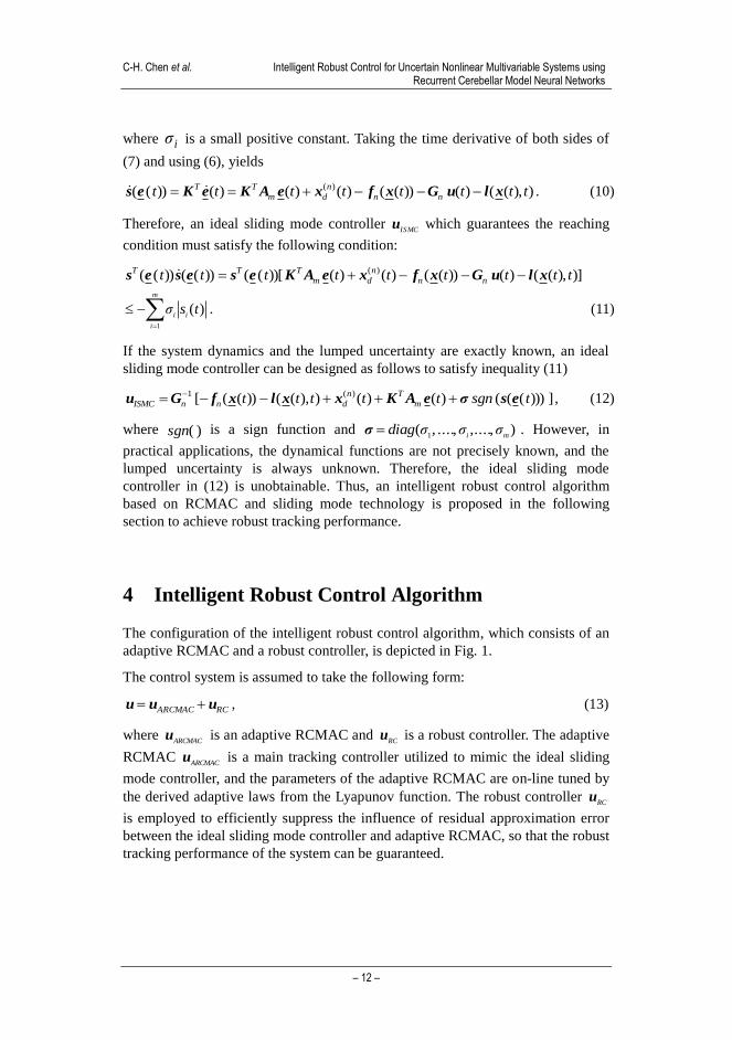
The configuration of the intelligent robust control algorithm, which consists of an
adaptive RCMAC and a robust controller, is depicted in Fig. 1.
The control system is assumed to take the following form:
RCARCMAC uuu , (13)
where ARCMAC
u is an adaptive RCMAC and RC
u is a robust controller. The adaptive
RCMAC ARCMAC
u is a main tracking controller utilized to mimic the ideal sliding
mode controller, and the parameters of the adaptive RCMAC are on-line tuned by
the derived adaptive laws from the Lyapunov function. The robust controller RC
u
is employed to efficiently suppress the influence of residual approximation error
between the ideal sliding mode controller and adaptive RCMAC, so that the robust
tracking performance of the system can be guaranteed.
Acta Polytechnica Hungarica Vol. 12, No. 5, 2015
– 13 –
Figure 1
The configuration of the intelligent robust control system
4.1 Description of RCMAC
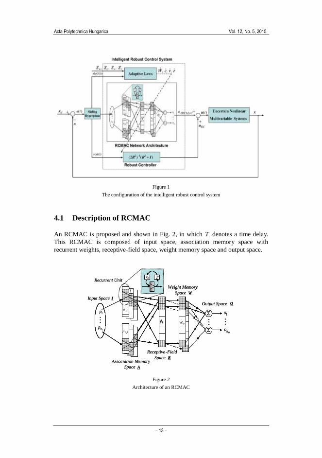
An RCMAC is proposed and shown in Fig. 2, in which T denotes a time delay.
This RCMAC is composed of input space, association memory space with
recurrent weights, receptive-field space, weight memory space and output space.
Input Space
Receptive -Field
Space
Weight Memory
Space
Association Memory
Space
Recurrent Unit
k1
nk
Output Space
kow
-
kpw anp
1p k1
kna
k
ikr Tikr
Ono
1o
I
A
R
W
O
Input Space
Receptive -Field
Space
Weight Memory
Space
Association Memory
Space
Recurrent Unit
k1
nk
Output Space
kow
-
kpw anp
1p k1
kna
k
ikr Tikrikr TTikr
Ono
1o
I
A
R
W
O
Figure 2
Architecture of an RCMAC

C-H. Chen et al. Intelligent Robust Control for Uncertain Nonlinear Multivariable Systems using Recurrent Cerebellar Model Neural Networks
– 14 –
The signal propagation and the basic function in each space are described as
follows.
1) Input space I : For a given a
a
nT
nppp ],,,[
21p , where
an is the
number of input state variables, each input state variable i
p must be quantized
into discrete regions (called elements) according to given control space. The
number of elements,e
n , is termed as a resolution.
2) Association memory space A : Several elements can be accumulated as a block,
the number of blocks, b
n , is usually greater than or equal to two. A denotes an
association memory space with c
n (bac
nnn ) components. In this space, each
block performs a receptive-field basis function, the Gaussian function is adopted
here as the receptive-field basis function, which can be represented as
2
2)(
ik
ikrik
ikv
cpexp , for
bnk ,2,1 , (14)
where ik
represents the output of the k-th receptive-field basis function for the i-
th input with the mean ik
c and variance . ik
v In addition, the input of this block
can be represented as
)()()( Ttrtptpikikirik
, (15)
where ik
r is the recurrent weight, and )( Ttik
denotes the value of ik
through
delay time T . It is clear that the input of this block contains the memory
term )( Ttik
, which stores the past information of the network and presents a
dynamic mapping. Figure 3 depicts the schematic diagram of a two-dimensional
RCMAC with 5e
n and 4f
n (f
n is the number of elements in a complete
block); in which 1
p is divided into blocks 1a
B and 1b
B , and 2
p is divided into
blocks 2a
B and 2b
B . By shifting each variable an element, different blocks will be
obtained. For instance, blocks 1c
B and 1d
B for 1
p , and blocks 2c
B and 2d
B for
2p are possible shifted elements for the second layer; and 1eB and 1fB for
1p ,
and 2eB and 2fB for 2
p for the third layer; and 1gB and 1hB for 1
p , and 2gB and
2hB for 2
p for the fourth layer. The receptive-field basis function ik
of each
block in this space has three adjustable parameters ik
c , ik
v and ik
r .

Acta Polytechnica Hungarica Vol. 12, No. 5, 2015
– 15 –
Variable
-0.9 -0.3 0.3 0.9
Layer 1
Layer 1Layer 2
Layer 2Layer 3
State (0.8, 0.8)
Layer 3
-1.5
1.5
Layer 4
Layer 4
-1.5 1.5
-0.9
-0.3
0.3
0.9
1p
2p
1aB1bB
1cB1dB
1eB 1fB
1gB 1hB
2aB
2bB
2cB
2dB
2eB
2fB2hB
2gB
21 bb BB
21 dd BB
21 ff BB
21 gg BB
Variable
11
15
12 16
13 17
1418
21
28
22
23
24
25
26
27
Variable
-0.9 -0.3 0.3 0.9
Layer 1
Layer 1Layer 2
Layer 2Layer 3
State (0.8, 0.8)
Layer 3
-1.5
1.5
Layer 4
Layer 4
-1.5 1.5
-0.9
-0.3
0.3
0.9
1p
2p
1aB1bB
1cB1dB
1eB 1fB
1gB 1hB
2aB
2bB
2cB
2dB
2eB
2fB2hB
2gB
21 bb BB
21 dd BB
21 ff BB
21 gg BB
Variable
11
15
12 16
13 17
1418
21
28
22
23
24
25
26
27
Figure 3
A two-dimensional RCMAC with 4fn and 5en
3) Receptive-field space R : Areas formed by blocks, referred to as 21 aa
BB and
21 bbBB are called receptive-fields. The number of receptive-fields, ,
dn is equal to
bn in this study. The k-th multi-dimensional receptive-field function is defined as
aa n
i ik
ikrik
n
i
ikkkkkv
cpexp
1
2
2
1
)(),,,( rvcp for
dnk ,2,1 , (16)
where a
a
nT
knkkkccc ],,,[
21c , a
a
nT
knkkkvvv ],,,[
21v and
a
a
nT
knkkkrrr ],,,[
21r . The multi-dimensional receptive-field functions can
be expressed in a vector form as
T
nk d
],,,,[),,,(1
rvcpΦ , (17)
where da
d
nnTT
n
T
k
T ],,,,[1
cccc , da
d
nnTT
n
T
k
T ],,,,[1
vvvv and
da
d
nnTT
n
T
k
T ],,,,[1
rrrr .
4) Weight memory space W : Each location of R to a particular adjustable value
in the weight memory space can be expressed as
od
oddd
o
o
o
nn
nnpnn
knkpk
np
np
www
www
www
1
1
1111
1],,,,[ wwwW , (18)

C-H. Chen et al. Intelligent Robust Control for Uncertain Nonlinear Multivariable Systems using Recurrent Cerebellar Model Neural Networks
– 16 –
where d
d
nT
pnkpppwww ],,[
1w , and
kpw denotes the connecting weight
value of the p-th output associated with the k-th receptive-field.
5) Output space O : The output of RCMAC is the algebraic sum of the activated
weights in the weight memory, and is expressed as
dn
k
kkp
T
ppwo
1
Φw , for o
np ,2,1 . (19)
The outputs of RCMAC can be expressed in a vector notation as
ΦWoTT
np O
ooo ],,[1
. (20)
In the two-dimensional case shown in Fig. 3, the output of RCMAC is the sum of
the value in receptive-fields 21 bb
BB , 21 dd
BB , 21 ff
BB and ,21 gg
BB where the input
state is (0.8,0.8). The architecture of RCMAC is designed to have the advantages
of simple structure with dynamic characteristics. The role of the recurrent loops is
to consider the past value of the receptive-field basis function in the association
memory space. Thus, this RCMAC has dynamic characteristics.
4.2 Robust Controller Design
Subtracting (12) from (10), yields
))](([ ][ ))(( tsgnt ISMCn esσuuGes . (21)
Assume there exists an optimal RCMAC *
ARCMACu to estimate the ideal sliding
mode controller ISMC
u such that
εΦWεrvcWpuu ******* ),,,,( T
ARCMACISMC, (22)
where T
mi] ,...., ,.... ,[
1ε is a minimum reconstructed error vector; *
W ,
,*Φ
*** and , rvc are the optimal parameter matrix and vectors of
,W ,Φ , and , rvc respectively. However, the optimal RCMAC cannot be
obtained; thus, an estimating RCMAC is used to estimate the optimal RCMAC.
From (20), the control law (13) can be rewritten as follows:
RC
T
RCARCMACt uΦWurvcWpuu ˆˆ)ˆ ,ˆ ,ˆ,ˆ,()( , (23)
where ,W ,Φ rvc ˆ and ˆ ,ˆ are the estimated matrix and vectors of
,*W ,*
Φ , and , ***rvc respectively. Thus, the dynamic equation (21) can be
expressed via (22) and (23) as
))](([ ] [ ))(( * tsgnt RCARCMACARCMACn esσuuεuGes

Acta Polytechnica Hungarica Vol. 12, No. 5, 2015
– 17 –
))](([ ]ˆˆ [ ** tsgnRC
TT
n esσuεΦWΦWG
))](([ ] ~ˆ~
[ * tsgnRC
TT
n esσuεΦWΦWG , (24)
where ΦΦΦWWW ˆ~ and ˆ~ ** . Moreover, the linearization technique is
employed to transform the multi-dimensional receptive-field basis functions into a
partially linear form. The expansion of Φ~
in Taylor series can be obtained as
βrr
r
r
r
vv
v
v
v
cc
c
c
c
Φrrvvcc
)ˆ(|)ˆ(|)ˆ(|
~
~
~
~ *
ˆ
1
*
ˆ
1
*
ˆ
1
1
T
n
T
k
T
T
n
T
k
T
T
n
T
k
T
n
k
dddd
βrΦvΦcΦ ~~~ rvc
, (25)
where ;|, , , , ˆ
1 dadd nnn
T
nk
c
ccccc
Φ
;|, , , , ˆ
1 dadd nnn
T
nk
v
vvvvv
Φ
dadd nnn
T
nk
r
rrrrr
Φ ˆ
1 |, , , ,
, ccc ˆ~ * ; vvv ˆ~ * ; rrr ˆ~ * and
dnβ is a vector of higher-order terms. Moreover,
c
k
, v
k
and r
k
are
defined as
]0,,0,,,,0,,0[
)(1)1(
ada
a nknkn
k
k
k
nk
k
cc
c , (26)
]0,,0,,,,0,,0[
)(1)1(
ada
a nknkn
k
k
k
nk
k
vv
v, (27)
]0,,0,,,,0,,0[
)(1)1(
ada
a nknkn
k
k
k
nk
k
rr
r. (28)
Rewriting (25), it can be obtained that
βrΦvΦcΦΦΦ ~~~ˆ*
rvc. (29)
C-H. Chen et al. Intelligent Robust Control for Uncertain Nonlinear Multivariable Systems using Recurrent Cerebellar Model Neural Networks
– 18 –
Substituting (25) and (29) into (24), yields
))](([ ])~~~(ˆ)~~~ˆ(~
[ ))(( tsgnt RCrvc
T
rvc
T
n esσuεβrΦvΦcΦWβrΦvΦcΦΦWGes
))](([ ])~~~(~
)~~~(ˆˆ~[ * tsgnRC
T
rvc
T
rvc
TT
n esσuεβWrΦvΦcΦWrΦvΦcΦWΦWG
))](([ ])~~~(ˆˆ~[ tsgnRCrvc
TT
n esσuωrΦvΦcΦWΦWG , (30)
where the approximation error .)~~~(~*
εrΦvΦcΦWβWω rvc
TT
In case of the existence of ,ω consider a specified
H tracking performance [18]
)0(~)0(~)]0(~
)0(~
[ )0()0( )( 111
1
0
2cΞcWΞWsGs
c
T
w
T
n
T
m
i
T
itrdtts
m
i
T
iir
T
v
T dtt1
0
2211 )()0(~)0(~)0(~)0(~ rΞrvΞv , (31)
where rvcw
ΞΞΞΞ and , , are diagonal positive constant learning-rate matrices,
and i is a prescribed attenuation constant. If the system starts with initial
conditions ,)0( 0s ,)0(~
0W ,)0(~ 0c ,)0(~ 0v ,)0(~ 0r then the
H tracking
performance in (31) can be rewritten as
m
ii
i
i
TL
ssup
i1][0,2
, (32)
where T
iidttss
0
22
)( and T
iidtt
0
22
. )( This shows that i is an attenuation
level between the approximation error )( ti
and system output function ).(tsi
If i , this is the case of minimum error tracking control without
approximation attenuation [18]. Therefore, the following theorem can be stated
and proved.
Theorem 1: Consider the nth-order multivariable nonlinear systems represented
by (1). The intelligent robust control system is defined as in (13), in which the
adaptive laws of RCMAC are designed as in (33)-(36) and the robust controller is
designed as in (37). Then, the robust tracking performance in (31) can be achieved
for the prescribed attenuation level ..., 2, 1, , mii , where R=diag[ 1 , 2 ,…,
m ] mm is a diagonal matrix.
))((ˆ ˆ tT
w esΦΞW
, (33)
))((ˆ ˆ tT
cc esWΦΞc , (34)
))((ˆ ˆ tT
vv esWΦΞv , (35)

Acta Polytechnica Hungarica Vol. 12, No. 5, 2015
– 19 –
))((ˆ ˆ tT
rr esWΦΞr , (36)
))(( )()(2 212 tRC esRRu I . (37)
Proof: The Lyapunov function candidate is given by
~~~~~~)~~
( ))(())(( 2
1)~,~,~,
~)),((( 11111
rΞrvΞvcΞcWΞWesGesrvcWes r
T
v
T
c
T
w
T
n
T trtttV .
(38)
Taking the derivative of the Lyapunov function and using (30), yields
vΞrvΞvcΞcWΞWesGesrvcWes ~~~~~~)~~
( ))(())(()~,~,~,~
)),((( 11111 r
T
v
T
c
T
w
T
n
T trtttV
))](([ ))((])~~~(ˆˆ~[ ))(( 1 tsgntt n
T
RCrvc
TTTesσGesuωrΦvΦcΦWΦWes
vΞrvΞvcΞcWΞW ˆ~ˆ~ˆ~)ˆ
~( 1111
r
T
v
T
c
T
w
Ttr (39)
It can be noted that )))(( ˆ~
(ˆ~ ))(( ttrt TTTT
esΦWΦWes and
0))](([ ))(( 1 tsgnt n
TesσGes , so (39) can be rewritten as
cΞesWΦcWΞesΦWrvcWes ˆ))(((ˆ~ ]ˆ))((( ˆ[~
)~,~,~,~
)),(((( 11
c
T
c
T
w
TT tttrtV
]))((())((([ ˆ))(((ˆ~ ˆ))(((ˆ~ 11
RC
TT
r
T
r
T
v
T
v
T tttt uesωesrΞesWΦrvΞesWΦv .
(40)
From (33)-(36) and using (37), (40) can be rewritten as
m
i i
iiii tsttstV
12
22 ]
2
1)()()([ )~,~,~,
~,)((
rvcWs
] 2
)(
2
)()()([
12
22
m
i i
iiii
tststts
] 2
)())(
)((
2
1
2
)([
22
1
22 t
ttsts ii
m
iii
i
ii
] 2
)(
2
)([
22
1
2 tts iim
i
i
. (41)
Assuming ),[0, ],[0, 2
TTLi
integrating the above equation
from 0 t to , Tt yields
m
i
T
iiT
i dttdttsVTV1
0
22
0
2 ] )( 2
)(2
1[(0))(
. (42)

C-H. Chen et al. Intelligent Robust Control for Uncertain Nonlinear Multivariable Systems using Recurrent Cerebellar Model Neural Networks
– 20 –
Since 0)( TV , the above inequality implies the following inequality
m
i
T
ii
m
i
T
i dttVdtts1
0
22
1
0
2 )(2
1(0) )(
2
1 . (43)
Using (38), the above inequality is equivalent to the following
)0(~)0(~)]0(~
)0(~
[ )0()0( )( 111
1
0
2cΞcWΞWsGs
c
T
w
T
n
T
m
i
T
itrdtts
m
i
T
iir
T
v
T dtt1
0
2211 )()0(~)0(~)0(~)0(~ rΞrvΞv . (44)
Thus the proof is completed.
5 Simulation Results
To illustrate the effectiveness of the proposed control system, it is applied to control
a Chua’s chaotic circuit and a three-links robot manipulator. Moreover, an adaptive
fuzzy neural network controller (AFNNC) [19] and the proposed RCMAC are
applied to these two systems for comparison.
Example 1: Chua’s chaotic circuit
A typical Chua’s chaotic circuit consists of one linear resistor ( R ), two capacitors
(1
C ,2
C ), one inductor ( L ) and one nonlinear resistor ( )(1C
vg ) as shown in Fig. 4.
R
1C1Cv
Li
L
3u2u
2C2Cv g
1u
Figure 4
Chua’s chaotic circuit
The dynamic equations of the Chua’s circuit are written as [20]
)()()()(11
11
1
1121
tdtuvgvvRC
vCCCC
, (45)
)()()(11
22
2
212
tdtuivvRC
vLCCC
, (46)
Acta Polytechnica Hungarica Vol. 12, No. 5, 2015
– 21 –
)())((1
332
tdtuvL
iCL
, (47)
where ])( ,)( ,)([)( 321
Ttututut u denotes the control input
and Ttdtdtdt ])( ,)( ,)([)( 321d denotes the external disturbance. The
voltages ),( 1
tvC
)(2
tvC
and the current )( tiL
are the state variables. Thus, the state
vector of chaotic system is defined as
.])( ,)( ,)([)]( ),( ),([)( 32121
TT
LCC txtxtxtitvtvt x The dynamic equation (45)-
(47) can be rewritten as
)()()()()( ttt duxGxfx , (48)
where
)(1
)(1
1
)()(11
)(
2
21
112
2
1
C
LCC
CCC
vL
ivvRC
vgvvRC
xf and
100
01
0
001
)(2
1
L
C
C
diagxG .
The external disturbance is given as .
2.0)2.0()(3
5.0)2.0()(2
3.0)2.0( )(2
)(
)(
)(
)(
3
2
1
texptsin
texptcos
texptsin
td
td
td
td
The physical parameters of chaotic circuit are assumed as
,Δ0
RRR ,)(Δ)()( 111 0 CCC
vgvgvg ,Δ 0
LLL ,Δ 1011
CCC
,Δ 2202
CCC where , 0
R 0100
, ,)(1
CLvgC
and 20
C are the nominal values and
1Δ ,Δ ,)(Δ ,Δ
1
CLvgRC
and 2
ΔC denote the unknown nonlinear time-varying
perturbations [19]. The nominal values are given as
0.5. 1, 1, ,0.02)( 5,20010
3
00 111
CCLvvvgRCCC
The time-varying
perturbations are ,)(0.2)(Δ /2),(Δ11 CC
vtsinvgtsinR
0.1Δ /2),(0.10.1Δ 0.15,Δ21 CtcosCL . The desired trajectories come
from the reference model outputs that are chosen as ididi
txtx 4)(4)( ,
wherei is the input signal to the reference model. The initial conditions of the
Chua’s chaotic circuit and the reference models are given as
,1)0(1
x 1.)0( and ,1)0( 0,)0( 0,)0( and 0)0(32132
ddd
xxxxx The
reference inputs are unit periodic rectangular signals. For the proposed control
scheme, the sliding hyperplane is design as ).( ))(( tt ees The proposed RCMAC
is characterized as:

C-H. Chen et al. Intelligent Robust Control for Uncertain Nonlinear Multivariable Systems using Recurrent Cerebellar Model Neural Networks
– 22 –
number of input state variables: 3a
n ,
number of elements for each state variable: 5e
n (elements),
generalization: 4f
n (elements/ block),
number of blocks for each state variable: 2b
n (blocks/layer) 4 (layer)
8 (blocks),
number of receptive-fields: 2d
n (receptive-fields/layer) 4 (layer)
8 (receptive-fields),
receptive-field basis functions: ]/)([ 22
ikikrikikvcpexp for 3 2, 1,i and
.8,,2,1 k
The inputs of RCMAC are )(1
ts , )(2
ts and );( 3
ts while the input spaces of input
signals are normalized within ]}2,2][2,2[]2,2{[ . The initial means of the
Gaussian functions are divided equally and are set as
]8.2,2,2.1,4.0,4.0,2.1,2,8.2[],,,,, ,,[87654321
iiiiiiii
cccccccc and the
initial variances are set as 1.6ik
v for 3 2, 1,i and 8,,2,1 k . The learning-
rate matrices of RCMAC are selected as 242488
5.0 ,30
IΞΞΞIΞrvcw
and the specified attenuation constant diagonal matrix is .2.0 33
IR
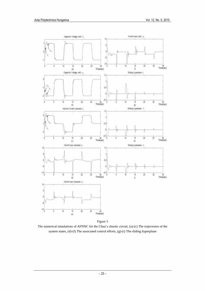
The simulation results of AFNNC for the Chua’s chaotic circuit are shown in Fig.
5. The trajectories of the system states are plotted in Figs. 5(a)-(c) for )(1
tvC
,
)(2
tvC
and )(tiL
, respectively. The associated control efforts )( ,)( ,)(321
tututu are
depicted in Figs. 5(d)-(f). Moreover, the sliding hyperplanes )( 1
ts , )(2
ts and )( 3
ts
are shown in Figs. 5(g)-(i). The simulation results of RCMAC for the Chua’s
chaotic circuit are shown in Fig. 6. The trajectories of the system states are plotted
in Figs. 5(a)-(c) for )(1
tvC
, )(2
tvC
and )(tiL
, respectively. The associated control
efforts )( ,)( ,)(321
tututu are depicted in Figs. 6(d)-(f). Moreover, the sliding
hyperplanes )( 1
ts , )(2
ts and )( 3
ts are shown in Figs. 6(g)-(i). From the
simulation results, it can be seen that the proposed RCMAC can provide better
control performance with smaller tracking error than the AFNNC.
Acta Polytechnica Hungarica Vol. 12, No. 5, 2015
– 23 –
Figure 5
The numerical simulations of AFNNC for the Chua’s chaotic circuit, (a)-(c) The trajectories of the
system states, (d)-(f) The associated control efforts, (g)-(i) The sliding hyperplane

C-H. Chen et al. Intelligent Robust Control for Uncertain Nonlinear Multivariable Systems using Recurrent Cerebellar Model Neural Networks
– 24 –
Control input (volt) 3 u
Time (sec)(f)
Time (sec)(g)
Sliding hyperplane 1 s
Time (sec)(h)
Sliding hyperplane 2 s
Time (sec)(i)
Sliding hyperplane 3 s
Time (sec)
Inductor current (ampere) Li
(c)
3 x
3 dx
Capacitor voltage (volt)1
Cv
Time (sec)(a)
1 x
1 dx
Capacitor voltage (volt) 2
Cv
Time (sec)(b)
2 x2 dx
Time (sec)
Control input (ampere) 1 u
(d)
Control input (ampere) 2 u
Time (sec)(e)
Figure 6
The numerical simulations of RCMAC for the Chua’s chaotic circuit, (a)-(c) The trajectories of the
system states, (d)-(f) The associated control efforts, (g)-(i) The sliding hyperplane

Acta Polytechnica Hungarica Vol. 12, No. 5, 2015
– 25 –
Example 2: A three-links robot manipulator
)(1
tq
)(1
t
)(2
t
)(3
t
)(2
tq
)(3
tq
1m
2m
3m
)(1
tq
)(1
t
)(2
t
)(3
t
)(2
tq
)(3
tq
1m
2m
3m
Figure 7
A three-links robot manipulator
A three-links robot manipulator is depicted as Fig. 7. The dynamic equation is
given as follows [21]:
ττqgqqqCqqM d
)(),()( , (49)
where
111
011
001
2
22
222
)(
336235
36336223524
36235336242235241
dcdcd
cddcddcdcd
cdcddcdcddcdcdd
qM ,
0)(
)(),(
21363623612351
321363632351241363
362361
2351363
23532352
2351241
2353363
2352242
3632353
2352242
qqsdsdqsdqsdq
qqqsdsdqsdqsdqsdq
sdqsdq
sdqsdq
sdqsdq
sdqsdq
sdqsdq
sdqsdq
sdqsdq
sdqsdq
qqC ,
gm
gm
gm
ca
cacaca
cacacacacaca
3
2
1
1233
1233122122
1233122111221111
2
100
22
1
2
10
2
1
2
1
2
1
)(qg and
)( 1.0
)2cos(1.0
)2(2.0
tsin
t
tsin
dτ .

C-H. Chen et al. Intelligent Robust Control for Uncertain Nonlinear Multivariable Systems using Recurrent Cerebellar Model Neural Networks
– 26 –
In (39), 3
321)]( ),(),([ Ttqtqtqq is the angular position vector, 3 , qq are
the joint velocity and acceleration vector, respectively, 33)( qM is the inertia
matrix, 3 τ is the input torque vector, 33),( qqC is the Coriolis/Centripetal
matrix, 3)( qg is the gravity vector, and 3 dτ is the external disturbance.
The acceleration of gravity is 2/ 8.9 smg . i
m is the link mass; i
a is the link
length; the short hand notations are defined as )(jiij
qqsins , )(jiij
qqcosc ;
and i
d is defined as in Table 1. In Table 1, i
i denotes the moment of inertia
( 2 mkg ). The detail data of system parameters are given in Table 1.
Table 1
The system parameters of robot manipulator
id ])25.0[(5.0
1
2
13211iammmd
21324]5.0[ aammd
])25.0[(5.02
2
2322iammd
31355.0 aamd
])25.0[(5.03
2
333iamd
32365.0 aamd
ia ma 5.0
1 ma 4.0
2 ma 3.0
3
im kgm 2.1
1 kgm 5.1
2 kgm 0.3
3
ii 23
1 1033.43 kgmi 23
2 1008.25 kgmi 23
3 1067.32 kgmi
The dynamic equation (52) can be expressed as
)()())(())(()( ttttt duxGxfx , (50)
where ,])( ),( ,)([)]( ),(),([Δ)(321321
TT txtxtxtqtqtqt x
)],(),()[())((1
qgqqqCqMxf t ),())((
1qMxG
t
dt τqMd )()(
1
and .])( ,)(,)([)( 3
321 Ttttt u The reference trajectories are described as a
reference model output and a sinusoid function at different time. When 2.11t
sec, the reference models are described as
, 63.111)(63.111)(13.21)(idididi
txtxtx for .3 ,2 ,1i The initial conditions
of the robot manipulator are given
as . 0)0( and 0)0( ,0)0( 0.2,)0( 0.1,)0( ,3.0)0( 321321
xxxxxx The
initial conditions of the reference models are given as
. 0)0( and 0)0( ,0)0( 0,)0( 0,)0( ,0)0( 321321
dddddd
xxxxxx The
reference inputs are unit periodic rectangular signals. When 2.11t sec, a
sinusoid function command is used. For the proposed control scheme, the sliding
hyperplane is designed as ).(10)( ))(( ttt eees The proposed RCMAC is
characterized as:
number of input state variables: 3a
n ,
number of elements for each state variable: 5e
n (elements),

Acta Polytechnica Hungarica Vol. 12, No. 5, 2015
– 27 –
generalization: 4f
n (elements/ block),
number of blocks for each state variable:
2b
n (blocks/layer) 4 (layer) 8 (blocks),
number of receptive-fields: 2d
n (receptive-fields/layer) 4 (layer)
8 (receptive-fields),
receptive-field basis functions: ]/)([ 22
ikikrikikvcpexp for 3 2, 1,i and
.8,,2,1 k
The inputs of RCMAC are )(1
ts , )(2
ts and );(3
ts while the input spaces of input
signals are normalized within ]}5.1,5.1][5.1,5.1[]5.1,5.1{[ . The initial means
of the Gaussian functions are divided equally and are set as
]1.2,5.1,9.0,3.0,3.0,9.0,5.1,1.2[],,,,, ,,[87654321
iiiiiiii
cccccccc and the
initial variances are set as 1.2ik
v for 3 2, 1,i and 8,,2,1 k . The learning-
rate matrices of RCMAC are chosen as 242488
05.0 ,50
IΞΞΞIΞrvcw
and the specified attenuation constant diagonal matrix .35.033
IR The
simulation results of AFNNC for the three-links robot manipulator are shown in
Fig. 8. The trajectories of the system states are plotted in Figs. 8(a)-(f) for
),(1
tq ),(2
tq ),(3
tq ),(1
tq )(2
tq and ),(3
tq respectively. The associated control
efforts )( ,)( ,)(321
tututu are depicted in Figs. 8(g)-(i). Moreover, the sliding
hyperplanes )(1
ts , )(2
ts and )(3
ts are shown in Figs. 8(j)-(l).

C-H. Chen et al. Intelligent Robust Control for Uncertain Nonlinear Multivariable Systems using Recurrent Cerebellar Model Neural Networks
– 28 –
Acta Polytechnica Hungarica Vol. 12, No. 5, 2015
– 29 –
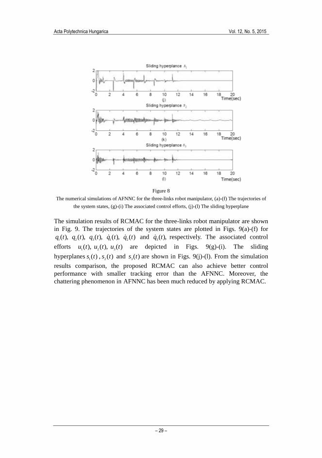
Figure 8
The numerical simulations of AFNNC for the three-links robot manipulator, (a)-(f) The trajectories of
the system states, (g)-(i) The associated control efforts, (j)-(l) The sliding hyperplane
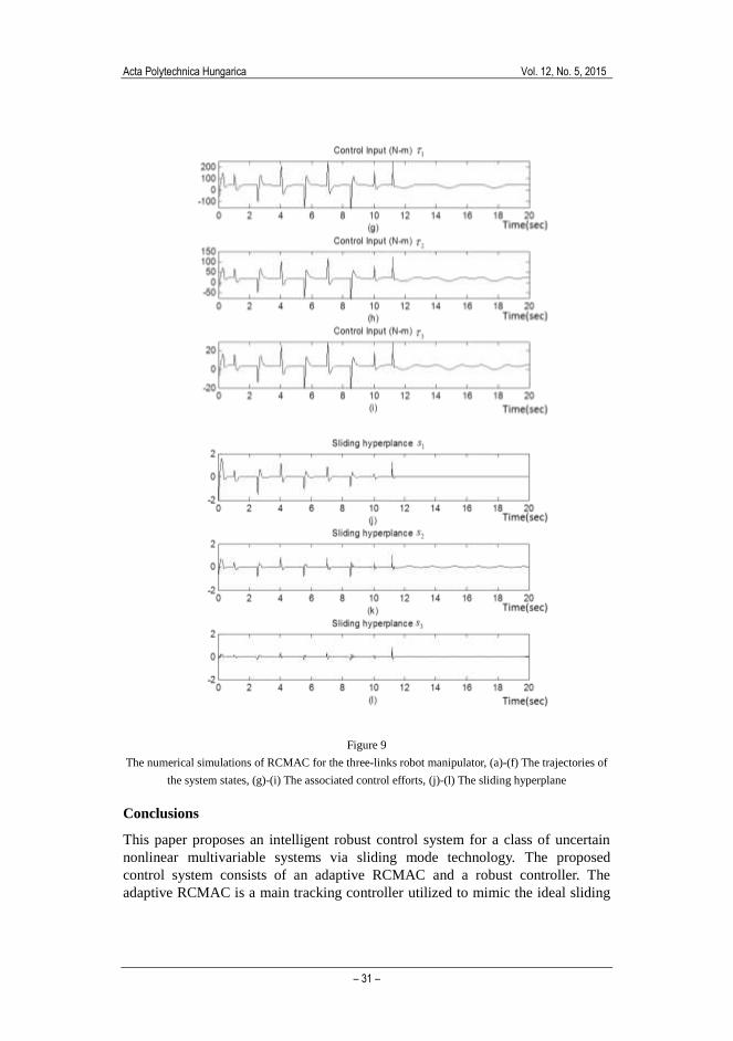
The simulation results of RCMAC for the three-links robot manipulator are shown
in Fig. 9. The trajectories of the system states are plotted in Figs. 9(a)-(f) for
),(1
tq ),(2
tq ),(3
tq ),(1
tq )(2
tq and ),(3
tq respectively. The associated control
efforts )( ,)( ,)(321
tututu are depicted in Figs. 9(g)-(i). The sliding
hyperplanes )(1
ts , )(2
ts and )(3
ts are shown in Figs. 9(j)-(l). From the simulation
results comparison, the proposed RCMAC can also achieve better control
performance with smaller tracking error than the AFNNC. Moreover, the
chattering phenomenon in AFNNC has been much reduced by applying RCMAC.

C-H. Chen et al. Intelligent Robust Control for Uncertain Nonlinear Multivariable Systems using Recurrent Cerebellar Model Neural Networks
– 30 –
Acta Polytechnica Hungarica Vol. 12, No. 5, 2015
– 31 –
Figure 9
The numerical simulations of RCMAC for the three-links robot manipulator, (a)-(f) The trajectories of
the system states, (g)-(i) The associated control efforts, (j)-(l) The sliding hyperplane
Conclusions
This paper proposes an intelligent robust control system for a class of uncertain
nonlinear multivariable systems via sliding mode technology. The proposed
control system consists of an adaptive RCMAC and a robust controller. The
adaptive RCMAC is a main tracking controller utilized to mimic the ideal sliding

C-H. Chen et al. Intelligent Robust Control for Uncertain Nonlinear Multivariable Systems using Recurrent Cerebellar Model Neural Networks
– 32 –
mode controller, and the parameters of the adaptive RCMAC are on-line tuned by
the derived adaptive law from a Lyapunov function. Based on the H control
approach, the robust controller is employed to efficiently suppress the influence of
residual approximation error between the ideal sliding mode controller and
adaptive RCMAC, so that the robust tracking performance of the system can be
guaranteed. Finally, the simulation results of two multivariable nonlinear systems
have demonstrated the effectiveness of the proposed control scheme.
References
[1] J. J. E. Slotine and W. P. Li, Applied Nonlinear Control. Englewood Cliffs,
NJ: Prentice-Hall, 1991
[2] C. M. Lin and Y. J. Mon, “Decoupling Control by Hierarchical Fuzzy
Sliding-Mode Controller,” IEEE Trans. Control Systems Technology, Vol.
13, No. 4, pp. 593-598, 2005
[3] C. M. Lin and C. F. Hsu, “Supervisory Recurrent Fuzzy Neural Network
Control of Wing Rock for Slender Delta Wings,” IEEE Trans. Fuzzy
Systems, Vol. 12, No. 5, pp. 733-742, 2004
[4] J. H. Park, S. H. Huh, S. H. Kim, S. J. Seo, and G. T. Park, “Direct Adaptive
Controller for Nonaffine Nonlinear Systems using Self-Structuring Neural
Networks,” IEEE Trans. Neural Networks, Vol. 16, No. 2, pp. 414-422,
2005
[5] C. F. Hsu, C. M. Lin and R. G. Yeh, “Supervisory Adaptive Dynamic RBF-
based Neural-Fuzzy Control System Design for Unknown Nonlinear
Systems,” Applied Soft Computing, Vol. 13, No. 4, pp. 1620-1626, 2013
[6] C. M. Lin, A. B. Ting, C. F. Hsu and
C. M. Chung, “Adaptive Control for
MIMO Uncertain Nonlinear Systems using Recurrent Wavelet Neural
Network,” International Journal of Neural Systems, Vol. 22, No. 1, pp.37-
50, 2012
[7] C. M. Lin and C. F. Hsu, “Neural-Network Hybrid Control for Antilock
Braking Systems,” IEEE Trans. Neural Networks, Vol. 14, No. 2, pp. 351-
359, 2003
[8] C. H. Tsai, H. Y. Chung, and F. M. Yu, “Neuro-Sliding Mode Control with
its Applications to Seesaw Systems,” IEEE Trans. Neural Networks, Vol. 15,
No. 1, pp. 124-134, 2004
[9] F. Da, “Decentralized Sliding Mode Adaptive Controller Design Based on
Fuzzy Neural Networks for Interconnected Uncertain Nonlinear Systems,”
IEEE Trans. Neural Networks, Vol. 11, No. 6, pp. 1471-1480, 2000
[10] J. S. Albus, “A New Approach to Manipulator Control: the Cerebellar
Model Articulation Controller (CMAC),” J. Dyn. Syst. Meas. Contr., Vol.
97, No. 3, pp. 220-227, 1975

Acta Polytechnica Hungarica Vol. 12, No. 5, 2015
– 33 –
[11] F. J. Gonzalez-Serrano, A. R. Figueiras-Vidal and A. Artes-Rodriguez,
“Generalizing CMAC Architecture and Training,” IEEE Trans. Neural
Networks, Vol. 9, No. 6, pp. 1509-1514, 1998
[12] J. C. Jan and S. L. Hung, “High-Order MS_CMAC Neural Network,” IEEE
Trans. Neural Networks, Vol. 12, No. 3, pp. 598-603, 2001
[13] C. M. Lin and Y. F. Peng, “Adaptive CMAC-based Supervisory Control for
Uncertain Nonlinear Systems,” IEEE Trans. Systems, Man, and
Cybernetics, Part B, Vol. 34, No. 2, pp. 1248-1260, 2004
[14] C. M. Lin and H. Y. Li, “A Novel Adaptive Wavelet Fuzzy Cerebellar
Model Articulation Control System Design for Voice Coil Motors,” IEEE
Trans. Industrial Electronics, Vol. 59, No. 4, pp. 2024-2033, 2012
[15] T. F. Wu, P. S. Tsai, F. R. Chang, and L. S. Wang, “Adaptive Fuzzy CMAC
Control for a Class of Nonlinear Systems with Smooth Compensation,” IEE
Proc.,-Control Theory and Applications, Vol. 153, No. 6, pp. 647-657, 2006
[16] C. H. Lee, F. Y. Chang and C. M. Lin, “An Efficient Interval Type-2 Fuzzy
CMAC for Chaos Time-Series Prediction and Synchronization,” IEEE
Trans. on Cybernetics, Vol. 44, No. 3, pp. 329-341, 2014
[17] C. M. Lin and H. Y. Li “Dynamic Petri Fuzzy Cerebellar Model
Articulation Control System Design for Magnetic Levitation System,”
IEEE Trans. Control Systems Tecchnology, Vol. 23, No. 2, pp. 693-699,
2015
[18] B. S. Chen, C. H. Lee, Y. C. Chang, “ H Tracking Design of Uncertain
Nonlinear SISO Systems: Adaptive Fuzzy Approach,” IEEE Trans. Fuzzy
Systems, Vol. 4, No. 1, pp. 32-43, 1996
[19] F. J. Lin and P. H. Shen, ”Adaptive Fuzzy-Neural-Network Control for a
DSP-based Permanent Magnet Linear Synchronous Motor Servo Drive,”
IEEE Transactions on Fuzzy Systems, Vol. 14, No. 4, pp. 481-495, 2006
[20] Y. C. Chang, “Robust H Control for a Class of Uncertain Nonlinear
Time-Varying Systems and Its Application,” IEE Proc.,-Control Theory and
Applications, Vol. 151, No. 5, pp. 601-609, 2004
[21] E. Kim, “Output Feedback Tracking Control of Robot Manipulators with
Model Uncertainty via Adaptive Fuzzy Logic,” IEEE Trans. Fuzzy Systems,
Vol. 12, No. 3, pp. 368-378, 2004
Top Related