1

Insights into transducer-plane streaming patterns in thin-layered acoustofluidic devices

Junjun Lei,* Martyn Hill† and Peter Glynne-Jones‡

Faculty of Engineering and the Environment, University of Southampton, Southampton, SO17 1BJ, UK

(Received xxxx)

While classical Rayleigh streaming, whose circulations are perpendicular to the transducer radiating surfaces, is well-

known, transducer-plane streaming patterns, in which vortices circulate parallel to the surface driving the streaming, have

been less widely discussed. Previously, a four-quadrant transducer-plane streaming pattern has been seen experimentally

and subsequently investigated through numerical modelling. In this paper, we show that by considering higher order three-

dimensional cavity modes of rectangular channels in thin-layered acoustofluidic manipulation devices, a wider family of

transducer-plane streaming patterns are found. As an example, we present a transducer-plane streaming pattern, which

consists of eight streaming vortices with each occupying one octant of the plane parallel to the transducer radiating

surfaces, which we call here eight-octant transducer-plane streaming. An idealised modal model is also presented to

highlight and explore the conditions required to produce rotational patterns. It is found that both standing and travelling

wave components are typically necessary for the formation of transducer-plane streaming patterns. In addition, other

streaming patterns related to acoustic vortices and systems in which travelling waves dominate are explored with

implications for potential applications.

DOI:

I. INTRODUCTION

Acoustic streaming is steady fluid motion driven by the

absorption of acoustic energy due to the interaction of

acoustic waves with the fluid medium or its solid boundaries.

Understanding the driving mechanisms of acoustic streaming

patterns within acoustofluidic devices is important in order to

precisely control it for the enhancement or suppression of

acoustic streaming for applications such as particle/cell

manipulation [1-8], heat transfer enhancement [9-12], non-

contact surface cleaning [13-17], microfluidic mixing [18-

27], and transport enhancement [28-35].

In most bulk micro-acoustofluidic particle and cell

manipulation systems of interest, the acoustic streaming

fields are dominated by boundary-driven streaming [36],

which is associated with acoustic dissipation in the viscous

boundary layer [37]. Theoretical work on boundary-driven

streaming was initiated by Rayleigh [38], and developed by

a series of modifications for particular cases [39-44], which

have paved the fundamental understanding of acoustic

streaming flows.

While Rayleigh streaming patterns (which have

streaming vortices with components perpendicular to the

driving boundaries) have been extensively studied [45-48],

we have recently explored the mechanisms behind four-

quadrant transducer-plane streaming [49] which generates

streaming vortices in planes parallel to the driving boundary,

and modal Rayleigh-like streaming [50] in which vortices

have a roll size greater than the quarter wavelength of the

main acoustic resonance and are driven by limiting velocities

(the value of the streaming velocity just outside the boundary

layer [41,49], on the boundaries perpendicular to the axis of

the main acoustic resonance). The expressions for the

limiting velocities have terms corresponding to acoustic

velocity gradients along each coordinate axis. Depending on

which of these is dominant, different acoustic streaming

patterns arise in thin-layered acoustofluidic devices [50],

corresponding to the rotational and irrotational features of,

respectively, the active and reactive intensity patterns in

acoustic fields [51]. The defining feature of transducer-plane

streaming is that its vorticity is driven by vorticity in the

limiting velocity patterns themselves.

In this paper, we first investigate higher order

transducer-plane streaming patterns in thin-layered

acoustofluidic manipulation devices. “Thin-layered” devices

are defined here as resonators in which the thickness of the

fluid layer (in the direction of the acoustic axis) is less that

1/20th of its lateral dimensions [50] and of the order of half

an acoustic wavelength. We introduce a new boundary-

driven streaming pattern observed in a thin-layered glass

capillary device and then investigate the underlying physics

of transducer-plane streaming with an analytical model in

order to gain insights into the contributions of standing and

travelling wave components, respectively.

ΙI. EIGHT-OCTANT TRANSDUCER-PLANE

STREAMING

The experiments were performed in a transducer-

capillary device using micro particle image velocimetery

(μpiv) system as shown in FIG. 1(a), similar to those we used

previously [49,50] (see [52] and details in the supplemental

material [53]). This acoustofluidic system is of interest as it

is used elsewhere in a blood and bacterial capture device

[1,2]. The measurements were performed within 𝑥𝑦

horizontal planes (see FIG. 1(a)). The investigation area was

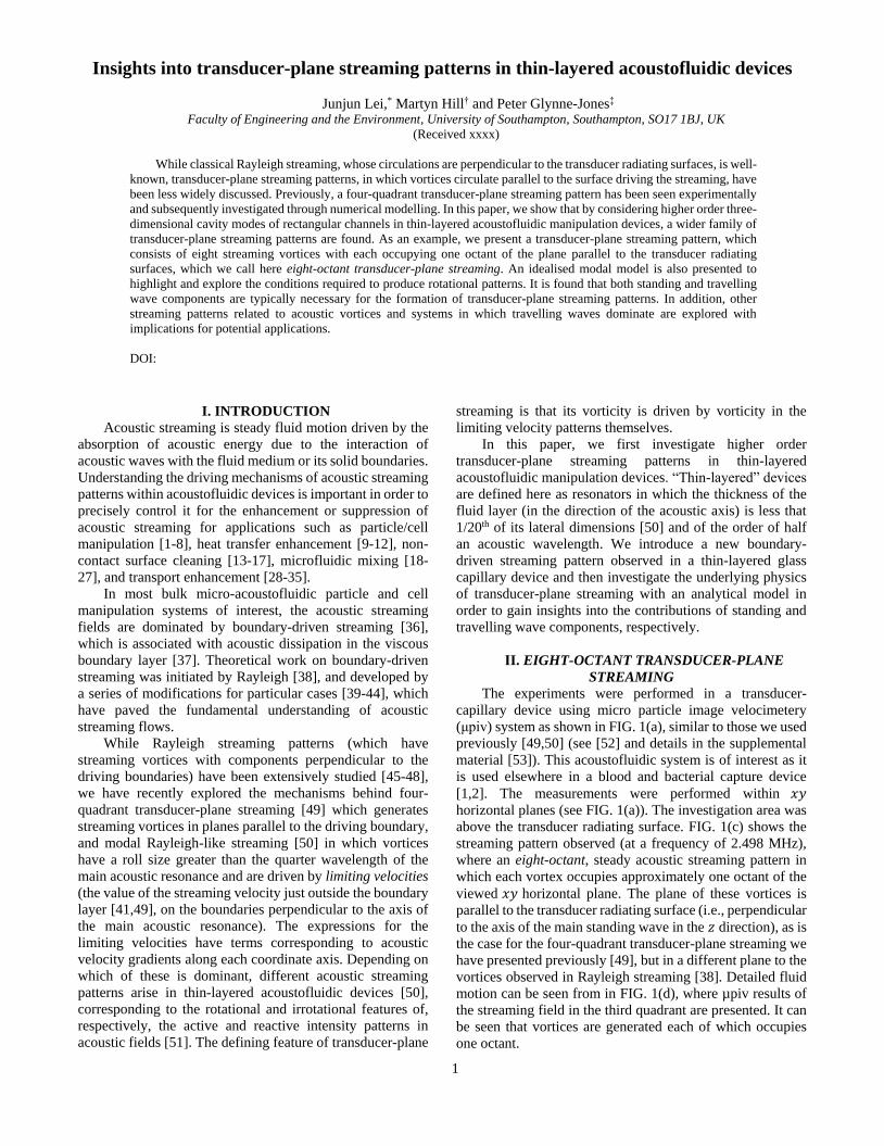
above the transducer radiating surface. FIG. 1(c) shows the

streaming pattern observed (at a frequency of 2.498 MHz),

where an eight-octant, steady acoustic streaming pattern in

which each vortex occupies approximately one octant of the

viewed 𝑥𝑦 horizontal plane. The plane of these vortices is

parallel to the transducer radiating surface (i.e., perpendicular

to the axis of the main standing wave in the 𝑧 direction), as is

the case for the four-quadrant transducer-plane streaming we

have presented previously [49], but in a different plane to the

vortices observed in Rayleigh streaming [38]. Detailed fluid

motion can be seen from in FIG. 1(d), where µpiv results of

the streaming field in the third quadrant are presented. It can

be seen that vortices are generated each of which occupies

one octant.

2

FIG. 1. (a) The experimental acoustofluidic particle manipulation device, where, to connect the capillary to plastic tubing, heat shrinkable

tubing (black) were used at the two ends of the capillary; (b) cross section of the device; (c) a photographic image of the distribution of beads

(radius of 1 µm) in the fluid after some minutes of streaming, where a main eight-octant transducer-plane streaming pattern can be seen in

which beads have agglomerated near the center of the streaming vortices and at the center of the device; (d) µpiv measurements of the eight-

octant transducer-plane streaming field in the third quadrant shown in (c) at a voltage of 30 Vp-p, where the arrow in the box shows a reference

velocity of 20 µm/s; (e) the considered 3D model (4 × 3 × 0.3 mm3), where the dash-dot lines show the symmetry planes; (f) the first-order

acoustic pressure field on all surfaces; (g) the 3D acoustic streaming velocity field, where velocity vectors are shown at two heights within

the chamber (𝑧 positions of one third and two thirds of the chamber height); and (h) the active intensity (i.e., the limiting velocity field) on

the driving boundaries (𝑧 = ±ℎ/2), where the five-pointed stars show the points of minimum pressure amplitude and normalized arrows are

used to show the flow directions.

To understand the driving mechanism of this eight-octant

transducer-plane streaming pattern, the finite element

package COMSOL [54] was used to model the acoustic and

streaming fields in the experimental device. In this work, we

have applied the limiting velocity method [41] based on the

perturbation method [44] to model the 3D outer streaming

fields in the capillary device. We have previously established

the viability of this method for solving 3D boundary-driven

streaming fields in thin-layered acoustofluidic manipulation

devices [48-50] and in vibrating plate systems [55].

III. Numerical model

The full numerical procedure can be split into three

steps. Firstly, the first-order acoustic fields within the devices

were modelled using the COMSOL ‘Pressure Acoustics,

Frequency Domain’ interface, which solves the harmonic,

linearized acoustic problems, taking the form:

∇2𝑝1 = −𝜔2

𝑐2𝑝1, (1)

where 𝑝1 is the complex acoustic pressure, 𝜔 is the angular

frequency and 𝑐 is the sound speed in the fluid. As the device

is symmetric to the centre, only a quarter of the fluid channel

was modelled here for numerical efficiency and the model is

located within coordinates: −𝑙 ≤ 𝑥 ≤ 0, −𝑤 ≤ 𝑦 ≤ 0,− ℎ 2⁄ ≤ 𝑧 ≤ ℎ 2⁄ (see FIG. 1(e)). Edges 𝑥 = 0 and 𝑦 = 0

were set as symmetric boundary conditions. We excited the

standing wave field through a ‘normal acceleration’

boundary condition on the bottom surface as published

previously [49,50]. Surface 𝑥 = −𝑙 was set as a plane wave

radiation condition in order to simulate the loss of acoustic

energy at the two ends of the fluid channel. The remaining

walls were modelled using sound reflecting boundary

conditions as these are water-glass interfaces and we are

working at frequencies away from resonances of these walls.

Secondly, the limiting velocities at all boundaries were

calculated as a function of the first-order acoustic velocity

fields. On planar surfaces normal to 𝑧, the limiting velocity

equations on the driving boundaries (𝑧 = ±ℎ/2) take the

form [49]:

𝑢𝐿 =−1

4𝜔Re {𝑞𝑥 + 𝑢1

∗ [(2 + 𝑖)∇ ∙ 𝒖𝟏

− (2 + 3𝑖)𝑑𝑤1

𝑑𝑧]},

(2a)

𝑣𝐿 =−1

4𝜔Re {𝑞𝑦 + 𝑣1

∗ [(2 + 𝑖)∇ ∙ 𝒖𝟏

− (2 + 3𝑖)𝑑𝑤1

𝑑𝑧]},

(2b)

𝑞𝑥 = 𝑢1

𝑑𝑢1∗

𝑑𝑥+ 𝑣1

𝑑𝑢1∗

𝑑𝑦, (2c)

𝑞𝑦 = 𝑢1

𝑑𝑣1∗

𝑑𝑥+ 𝑣1

𝑑𝑣1∗

𝑑𝑦, (2d)

where 𝑢𝐿 and 𝑣𝐿 are the two components of limiting

velocities along coordinates 𝑥 and 𝑦, Re represents the real

part of a complex value, and 𝑢1, 𝑣1 and 𝑤1 are components of

the complex first-order acoustic velocity vector, 𝒖𝟏, along

the coordinates 𝑥, 𝑦 and 𝑧, respectively. The superscript, ∗,

represents the complex conjugate.

Finally, this limiting velocity method was used to model

the acoustic streaming fields in this thin-layered

acoustofluidic device using the COMSOL ‘Creeping Flow’

interface. Outside of the acoustic boundary layer, the

governing equations for the second-order streaming

velocities, 𝒖𝟐, and the associated pressure fields, 𝑝2, are

∇𝑝2 = 𝜇∇2𝒖𝟐, (3a)

∇ ∙ 𝒖𝟐 = 0, (3b)

where 𝜇 is the dynamic viscosity of the fluid. Here, the

bottom and top surfaces (𝑧 = ±ℎ/2 ) were considered as

limiting velocity boundary conditions, surfaces 𝑥 = 0 and

𝑦 = 0 were symmetric conditions and the remaining surfaces

were no-slip boundary conditions.

3

The modeled acoustic pressure and acoustic streaming

fields at the resonant frequency 𝑓𝑟 = 2.4973 MHz (obtained

from a frequency sweep to find the frequency which gives the

maximum energy density in the cavity) in the 3D fluid

volumes are shown in FIG. 1(f-g). It can be seen from FIG.

1(g) that this quadrant model contained two dominant

streaming vortices with circulations parallel to the bottom

surface (i.e., the transducer radiating surface), which

compares well with the measured acoustic streaming

vortices, shown in FIG. 1(d).

The acoustic pressure field is shown in FIG. 1(f), a mode

with a half-wavelength in the 𝑧-direction of the model. The

fields along the 𝑥 and 𝑦 axes have approximately one and a

half- and one-wavelength variations respectively. The

rotational components of transducer-plane streaming are

closely linked to the active intensity field [49], which tends

to circulate about pressure nodal points [51,56]. The modeled

active intensity field in this case is shown in FIG. 1(h) and is

consistent with this, showing rotation at the boundary about

the two regions of minimum pressure amplitude on the

surface. These vortices thus drive the eight-octant transducer-

plane streaming patterns in the 𝑥𝑦 horizontal planes of the

3D fluid channels, with this higher order resonance

producing a higher order eight-octant vortex pattern in the

active sound intensity field in comparison with four-quadrant

streaming.

IV. ANALYTICAL MODEL We have previously presented results for transducer-

plane streaming in acoustofluidic devices [50], showing that

rotation in the active intensity is closely linked to the

rotational patterns seen in experiments. What was not made

clear previously was that a single standing wave mode does

not exhibit this rotation of active intensity. To achieve

rotational active intensity in a two-dimensional sound field it

is typically necessary to have a line or point pressure

minimum [56-58] This can result from the superposition of a

travelling and standing wave (see below) or of two standing

waves. This is supported with reference to our previous

models [48-50], where we find that if the radiation boundary

conditions (which allowed for the passage of energy across

them, but still reflected a proportion of that energy to create

combinations of standing and travelling waves), are replaced

with rigid or free boundary conditions, the rotational patterns

vanish. Hence in this section we create an analytical model to

study the streaming patterns resulting from simple

combinations of cavity modes and travelling modes for a case

that generates the four-quadrant transducer-plane streaming

patterns in order to obtain more insight into the relative

significance of the travelling and standing wave components,

and the effects of different modes and phase relationships.

In our model, the first-order acoustic pressure field, 𝑝1,

established in the fluid channel is decomposed into two

components, a standing wave component, 𝑝1𝑠, and a

travelling wave component (in the 𝑥-direction), 𝑝1𝑡,

𝑝1 = 𝑝1𝑠 + 𝑝1𝑡 , (4a)

𝑝1𝑠 = 𝑝0𝑠 cos(𝑘𝑥𝑠𝑥) cos(𝑘𝑦𝑠𝑦) sin(𝑘𝑧𝑠𝑧) 𝑒𝑖𝜔𝑡 , (4b)

𝑝1𝑡 = 𝑝0𝑡𝑒𝑖𝑘𝑥𝑡𝑥 cos(𝑘𝑦𝑡𝑦) sin(𝑘𝑧𝑡𝑧) 𝑒𝑖(𝜔𝑡+𝜑), (4c)

where subscripts 𝑠 and 𝑡 indicate the standing and travelling

wave components respectively, 𝑝0 is the acoustic pressure

amplitude, 𝜔 is the angular frequency and 𝜑 indicates the

phase difference between the standing and travelling wave

components. The wave numbers in the 𝑥, 𝑦 and 𝑧 directions

are 𝑘𝑥, 𝑘𝑦 and 𝑘𝑧. Each wave number has both a standing

and travelling wave component as indicated by the second s

or t subscripts.

As discussed above the standing (cavity) mode

components of equations 4 alone produce irrotational

limiting velocity fields but the combination of travelling and

standing wave components is the probable cause of the

patterns seen, as borne out by the correspondence between

modeled and experimental results. An example of the

streaming field created by an acoustic vortex formed from the

superposition of two standing wave modes is shown in FIG.

S2 in the supplemental material [52]. It is interesting to note

the applicability of the limiting velocity method in this case.

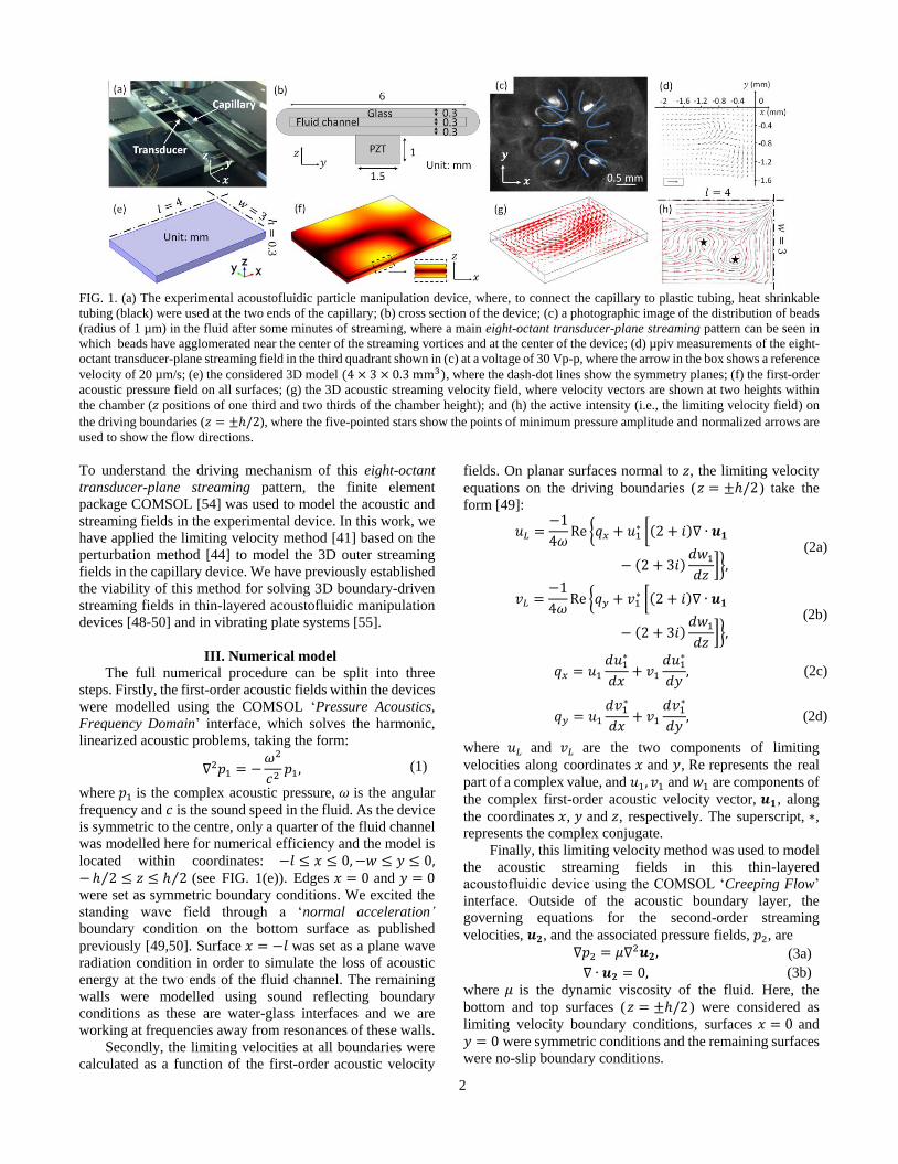
Here we take the four-quadrant streaming pattern as an

example (perhaps the simplest) to illustrate the roles of

respectively the standing and travelling wave components

[50]. The limiting velocity fields at the driving boundaries for

various combinations of standing and travelling wave

components were examined. It was found that the regular

four-quadrant vortex pattern is obtained for a combination of

the (1, 2, 1) standing wave mode and (t, 0, 1) travelling wave

mode, shown in FIG. 2.

The corresponding patterns with other travelling wave

components can be found in the supplemental material [52].

In a real device, combinations of these modes might be

FIG. 2. The active intensity (W/m2) and limiting velocity (m/s) fields at the driving boundaries for a combination of standing and travelling wave components (Pa). The phase difference between the standing and travelling wave components, φ = −π/2. The relationships between the four-quadrant transducer-plane streaming magnitudes, |𝒖𝟐|, the active intensity magnitudes |𝑰|, and the acoustic pressure amplitudes are shown in equation 5. Arrows in (c) and (d) show the corresponding vector fields.

4

excited, and it is interesting to note that the travelling wave

modes (t, n, 0) do not produce transducer-plane streaming,

and the higher order mode (t, 1, 1) can produce rotation in the

opposite direction. Real devices will exhibit complex

patterns and mode combinations that are less idealised than

those presented here, but we suspect that the higher order

modes are less likely to be exhibited in experimental devices.

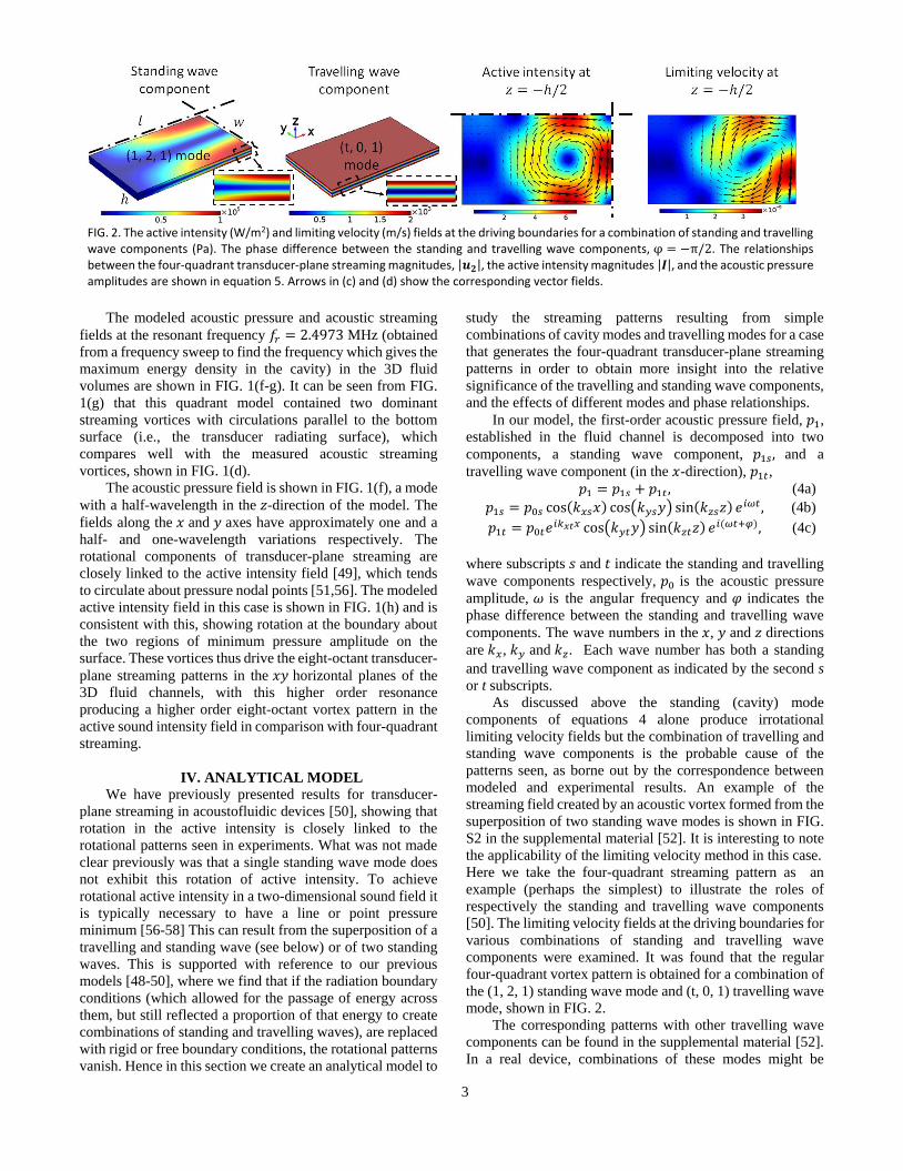
FIG 3 shows the transitions of streaming patterns from

various ratios of standing and travelling wave pressure

amplitudes. For very small values of 𝑝0𝑡 , modal Rayleigh-

like streaming patterns [50] are seen (FIG. 3(a)). As 𝑝0𝑡

increases, a gradual transition to the transducer-plane pattern

is seen (FIG. 3(b-c)). Ultimately as 𝑝0𝑡 approaches 𝑝0𝑠, irrotational terms become more dominant, leading to limiting

velocities which follow the predominantly 𝑥-directed active

intensity of the travelling wave (FIG. 3(d)), which would

drive flow if the end boundaries are allowed for the passage

of fluid.

For this specific mode, the limiting velocity (and hence

the magnitude of the transducer-plane streaming vortices) is

found to be approximately proportional (to within 5%) to that

of the active intensity following (see derivation in the

supplemental material [52])

|𝐼|𝑚𝑎𝑥 ≈𝑘𝑥𝑡𝑝0𝑡

2

2𝜌0𝜔(1 +

𝑝0𝑠

𝑝0𝑡). (5)

For 𝑝0𝑡 < 𝑝0𝑠 , increasing 𝑝0𝑡 shifts the vortex centre

outwards in the 𝑦-direction, while much larger values create

a pattern resembling the uniform active intensity which

follows the direction of propagation of the now dominant

travelling wave component. It was also found that

introducing a phase difference between the standing and

travelling wave components, 𝜑, shifts the vortex in the 𝑥-

direction.

We also note that the model shows that in situations

where the travelling wave component is dominant, the

limiting velocity at the boundary is non-zero. This will drive

a streaming pattern in addition to the (typically higher

velocity) Eckart streaming which will also be present in these

cases. Combinations of travelling waves in the x-direction

with standing modes in 𝑧 (or a pure travelling wave field)

reveal that the limiting velocity can take the opposite

direction to Eckart streaming in these cases, leading to

streaming vortices near the boundaries (see FIG. S3 in the

supplemental material [52]), as has been seen in a surface

acoustic wave device where the thickness of the fluid is at or

less than the viscous penetration depth [59].

In conclusion, we have demonstrated that a wider range

of transducer-plane streaming patterns exist other than the

four-quadrant pattern that had been observed previously,

related to higher order cavity modes. As an example, a new

pattern, eight-octant transducer-plane streaming, is both

predicted numerically and found experimentally in a glass

capillary device. We have created a simplified analytical

model to provide a deeper insight into the underlying physics

of transducer-plane streaming patterns in thin-layered

FIG. 3 The active intensity (W/m2) and limiting velocity (m/s) fields at the driving boundaries for a number of standing and travelling

wave components (Pa). The phase difference between the standing and travelling wave components, φ = −π/2.

5

acoustofluidic devices. The model highlights the importance

of having both standing and (typically smaller) travelling

wave components present within the acoustic cavity to create

rotational motion in the limiting velocity and resulting

streaming fields. We show that the limiting velocity method

also predicts the rotational streaming found from other

acoustic vortices. The model also highlights how fields with

stronger travelling wave components also exhibit boundary

driven streaming creating limiting velocities at the

boundaries which would not be found from pure Eckart

streaming, and that interactions between boundary-driven

streaming and Eckart streaming could create inner streaming

vortices.

This work was supported by the EPSRC/University of

Southampton Doctoral Prize Fellowship EP/N509747/1. PGJ

also acknowledges support from EPSRC Fellowship

EP/L025035/1. Models used to generate the simulation data,

and experimental data supporting this study are openly

available from the University of Southampton repository at

http://doi.org/10.5258/SOTON/D0119

*andyleiapply@gmail.com †m.hill@soton.ac.uk ‡p.glynne-jones@soton.ac.uk

[1] B. Hammarstrom, T. Laurell, and J. Nilsson, Seed particle-

enabled acoustic trapping of bacteria and nanoparticles in

continuous flow systems, Lab Chip 12, 4296 (2012).

[2] B. Hammarstrom, B. Nilson, T. Laurell, J. Nilsson, and S.

Ekstrom, Acoustic Trapping for Bacteria Identification in Positive

Blood Cultures with MALDI-TOF MS, Analytical chemistry 86,

10560 (2014).

[3] S. K. Chung and S. K. Cho, On-chip manipulation of objects

using mobile oscillating bubbles, J Micromech Microeng 18,

125024 (2008).

[4] B. R. Lutz, J. Chen, and D. T. Schwartz, Hydrodynamic

tweezers: 1. Noncontact trapping of single cells using steady

streaming microeddies, Analytical chemistry 78, 5429 (2006).

[5] S. Yazdi and A. M. Ardekani, Bacterial aggregation and

biofilm formation in a vortical flow, Biomicrofluidics 6, 044114

(2012).

[6] M. Antfolk, P. B. Muller, P. Augustsson, H. Bruus, and T.

Laurell, Focusing of sub-micrometer particles and bacteria enabled

by two-dimensional acoustophoresis, Lab Chip 14, 2791 (2014).

[7] C. Wang, S. V. Jalikop, and S. Hilgenfeldt, Size-sensitive

sorting of microparticles through control of flow geometry, Appl

Phys Lett 99, 034101 (2011).

[8] C. Devendran, I. Gralinski, and A. Neild, Separation of

particles using acoustic streaming and radiation forces in an open

microfluidic channel, Microfluidics and Nanofluidics 17, 879

(2014).

[9] M. Nabavi, K. Siddiqui, and J. Dargahi, Effects of transverse

temperature gradient on acoustic and streaming velocity fields in a

resonant cavity, Appl Phys Lett 93, 051902 (2008).

[10] B. G. Loh, S. Hyun, P. I. Ro, and C. Kleinstreuer, Acoustic

streaming induced by ultrasonic flexural vibrations and associated

enhancement of convective heat transfer, J Acoust Soc Am 111, 875

(2002).

[11] S. Hyun, D. R. Lee, and B. G. Loh, Investigation of convective

heat transfer augmentation using acoustic streaming generated by

ultrasonic vibrations, Int J Heat Mass Tran 48, 703 (2005).

[12] M. K. Aktas, B. Farouk, and Y. Q. Lin, Heat transfer

enhancement by acoustic streaming in an enclosure, J Heat Trans-T

Asme 127, 1313 (2005).

[13] W. Kim, T. H. Kim, J. Choi, and H. Y. Kim, Mechanism of

particle removal by megasonic waves, Appl Phys Lett 94, 081908

(2009).

[14] E. Maisonhaute, C. Prado, P. C. White, and R. G. Compton,

Surface acoustic cavitation understood via nanosecond

electrochemistry. Part III: shear stress in ultrasonic cleaning,

Ultrason Sonochem 9, 297 (2002).

[15] S. K. R. S. Sankaranarayanan, S. Cular, V. R. Bhethanabotla,

and B. Joseph, Flow induced by acoustic streaming on surface-

acoustic-wave devices and its application in biofouling removal: A

computational study and comparisons to experiment, Phys Rev E

77, 066308 (2008).

[16] A. A. Busnaina, I. I. Kashkoush, and G. W. Gale, An

Experimental-Study of Megasonic Cleaning of Silicon-Wafers, J

Electrochem Soc 142, 2812 (1995).

[17] M. Keswani, S. Raghavan, P. Deymier, and S. Verhaverbeke,

Megasonic cleaning of wafers in electrolyte solutions: Possible role

of electro-acoustic and cavitation effects, Microelectron Eng 86,

132 (2009).

[18] D. Ahmed, X. L. Mao, J. J. Shi, B. K. Juluri, and T. J. Huang,

A millisecond micromixer via single-bubble-based acoustic

streaming, Lab Chip 9, 2738 (2009).

[19] K. Sritharan, C. J. Strobl, M. F. Schneider, A. Wixforth, and Z.

Guttenberg, Acoustic mixing at low Reynold's numbers, Appl Phys

Lett 88, 054102 (2006).

[20] R. Shilton, M. K. Tan, L. Y. Yeo, and J. R. Friend, Particle

concentration and mixing in microdrops driven by focused surface

acoustic waves, J Appl Phys 104, 014910 (2008).

[21] T. D. Luong, V. N. Phan, and N. T. Nguyen, High-throughput

micromixers based on acoustic streaming induced by surface

acoustic wave, Microfluidics and Nanofluidics 10, 619 (2011).

[22] T. Frommelt, M. Kostur, M. Wenzel-Schafer, P. Talkner, P.

Hanggi, and A. Wixforth, Microfluidic mixing via acoustically

driven chaotic advection, Phys Rev Lett 100, 034502 (2008).

[23] R. H. Liu, J. N. Yang, M. Z. Pindera, M. Athavale, and P.

Grodzinski, Bubble-induced acoustic micromixing, Lab Chip 2, 151

(2002).

[24] G. G. Yaralioglu, I. O. Wygant, T. C. Marentis, and B. T.

Khuri-Yakub, Ultrasonic mixing in microfluidic channels using

integrated transducers, Analytical chemistry 76, 3694 (2004).

[25] M. K. Tan, L. Y. Yeo, and J. R. Friend, Rapid fluid flow and

mixing induced in microchannels using surface acoustic waves, Epl-

Europhys Lett 87, 47003 (2009).

[26] D. Ahmed, X. L. Mao, B. K. Juluri, and T. J. Huang, A fast

microfluidic mixer based on acoustically driven sidewall-trapped

microbubbles, Microfluidics and Nanofluidics 7, 727 (2009).

[27] C. Suri, K. Takenaka, Y. Kojima, and K. Koyama,

Experimental study of a new liquid mixing method using acoustic

streaming, J Chem Eng Jpn 35, 497 (2002).

[28] B. Moudjed, V. Botton, D. Henry, S. Millet, J. P. Garandet, and

H. Ben Hadid, Oscillating acoustic streaming jet, Appl Phys Lett

105, 184102 (2014).

[29] R. H. Nilson and S. K. Griffiths, Enhanced transport by

acoustic streaming in deep trench-like cavities, J Electrochem Soc

149, G286 (2002).

[30] T. Maturos et al., Enhancement of DNA hybridization under

acoustic streaming with three-piezoelectric-transducer system, Lab

Chip 12, 133 (2012).

[31] P. H. Huang et al., A reliable and programmable acoustofluidic

pump powered by oscillating sharp-edge structures, Lab Chip 14,

4319 (2014).

6

[32] D. Moller, T. Hilsdorf, J. T. Wang, and J. Dual, Acoustic

Streaming Used to Move Particles in a Circular Flow in a Plastic

Chamber, Aip Conf Proc 1433, 775 (2012).

[33] R. M. Moroney, R. M. White, and R. T. Howe, Microtransport

Induced by Ultrasonic Lamb Waves, Appl Phys Lett 59, 774 (1991).

[34] N. Li, J. H. Hu, H. Q. Li, S. Bhuyan, and Y. J. Zhou, Mobile

acoustic streaming based trapping and 3-dimensional transfer of a

single nanowire, Appl Phys Lett 101, 093113 (2012).

[35] M. Miansari and J. R. Friend, Acoustic Nanofluidics via

Room-Temperature Lithium Niobate Bonding: A Platform for

Actuation and Manipulation of Nanoconfined Fluids and Particles,

Adv Funct Mater 26, 7861 (2016).

[36] M. Wiklund, R. Green, and M. Ohlin, Acoustofluidics 14:

Applications of acoustic streaming in microfluidic devices, Lab

Chip 12, 2438 (2012).

[37] H. Bruus, Acoustofluidics 10: Scaling laws in acoustophoresis,

Lab Chip 12, 1578 (2012).

[38] Lord Rayleigh, On the circulation of air observed in Kundt's

tube, and on some allied acoustical problems., Phil. Trans. 175, 1

(1884).

[39] H. Schlichting, Berechnung ebener periodischer

Grenzschichtstromungen (Calculation of plane periodic boundary

layer streaming), Physikalische Zeitschrift 33, 327 (1932).

[40] P. J. Westervelt, The theory of steady rotational flow generated

by a sound field, J. Acoust. Soc. Am. 25, 60 (1952).

[41] W. L. Nyborg, Acoustic streaming near a boundary, J. Acoust.

Soc. Am. 30, 329 (1958).

[42] J. Lighthill, Acoustic Streaming, J Sound Vib 61, 391 (1978).

[43] M. F. Hamilton, Y. A. Ilinskii, and E. A. Zabolotskaya,

Acoustic streaming generated by standing waves in two-

dimensional channels of arbitrary width, J Acoust Soc Am 113, 153

(2003).

[44] S. S. Sadhal, Acoustofluidics 13: Analysis of acoustic

streaming by perturbation methods Foreword, Lab Chip 12, 2292

(2012).

[45] M. K. Aktas and B. Farouk, Numerical simulation of acoustic

streaming generated by finite-amplitude resonant oscillations in an

enclosure, J Acoust Soc Am 116, 2822 (2004).

[46] P. B. Muller, R. Barnkob, M. J. H. Jensen, and H. Bruus, A

numerical study of microparticle acoustophoresis driven by acoustic

radiation forces and streaming-induced drag forces, Lab Chip 12,

4617 (2012).

[47] P. B. Muller, M. Rossi, A. G. Marin, R. Barnkob, P.

Augustsson, T. Laurell, C. J. Kahler, and H. Bruus, Ultrasound-

induced acoustophoretic motion of microparticles in three

dimensions, Phys Rev E 88, 023006 (2013).

[48] J. Lei, M. Hill, and P. Glynne-Jones, Numerical simulation of

3D boundary-driven acoustic streaming in microfluidic devices, Lab

Chip 14, 532 (2014).

[49] J. Lei, P. Glynne-Jones, and M. Hill, Acoustic streaming in the

transducer plane in ultrasonic particle manipulation devices, Lab

Chip 13, 2133 (2013).

[50] J. J. Lei, P. Glynne-Jones, and M. Hill, Modal Rayleigh-like

streaming in layered acoustofluidic devices, Phys Fluids 28, 012004

(2016).

[51] F.J.Fahy, Sound intensity (E & FN Spon, London, 1995),

Second Edition edn.

[52] mpiv - MATLAB PIV Toolbox,

http://www.oceanwave.jp/softwares/mpiv/.

[53] See supplemental information at [URL will be inserted by

publisher] for the experimental method, numerical method,

derivation of active intensities and additional streaming patterns.

[54] COMSOL Multiphysics 4.4, (COMSOL Multiphysics 4.4)

http://www.comsol.com/.

[55] J. Lei, Formation of inverse Chladni patterns in liquids at

microscale: roles of acoustic radiation and streaming-induced drag

forces, Microfluidics and Nanofluidics 21, 50 (2017).

[56] J. A. Mann, J. Tichy, and A. J. Romano, Instantaneous and

Time-Averaged Energy-Transfer in Acoustic Fields, J Acoust Soc

Am 82, 17 (1987).

[57] R. V. Waterhouse, D. G. Crighton, and J. E. Ffowcs-Williams,

A Criterion for an Energy Vortex in a Sound Field, J Acoust Soc

Am 81, 1323 (1987).

[58] Z. Y. Hong, J. Zhang, and B. W. Drinkwater, Observation of

Orbital Angular Momentum Transfer from Bessel-Shaped Acoustic

Vortices to Diphasic Liquid-Microparticle Mixtures, Phys Rev Lett

114, 214301 (2015).

[59] A. R. Rezk, O. Manor, L. Y. Yeo, and J. R. Friend, Double

flow reversal in thin liquid films driven by megahertz-order surface

vibration, P Roy Soc a-Math Phy 470, 20130765 (2014).