


Languages
Pages
Legal


Forecasting Hurricane Intensity: Lessons from
Application of the Coupled Hurricane Intensity Prediction
System (CHIPS)
Images on pages 9, 35, 36, 37, 39, 40, 43, 55, and 60 are copyrighted by Oxford, NY: Oxford University Press, 2005. Book title is Divine wind: the history and science of hurricanes. ISBN: 0195149416. Used with permission.
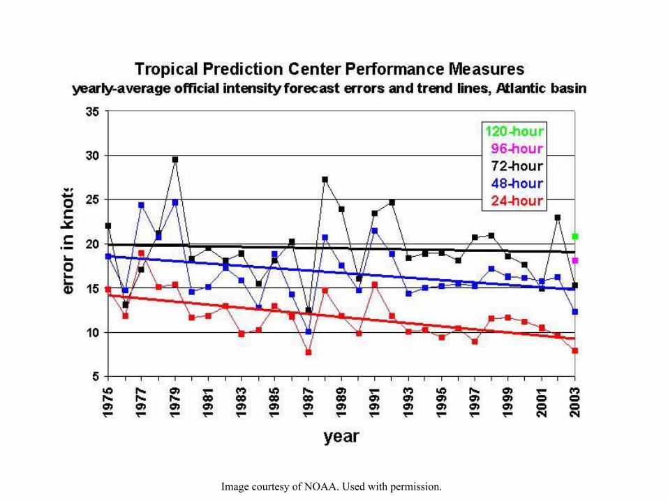
Image courtesy of NOAA. Used with permission.
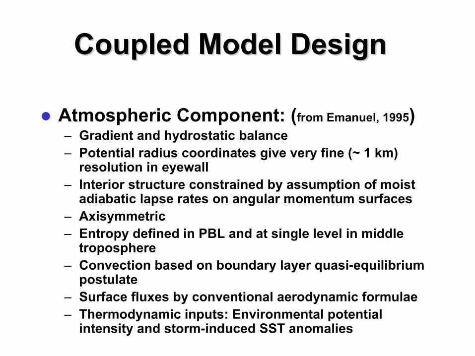
Coupled Model DesignCoupled Model Design
z Atmospheric Component: (from Emanuel, 1995) – Gradient and hydrostatic balance – Potential radius coordinates give very fine (~ 1 km)
resolution in eyewall – Interior structure constrained by assumption of moist
adiabatic lapse rates on angular momentum surfaces – Axisymmetric – Entropy defined in PBL and at single level in middle
troposphere – Convection based on boundary layer quasi-equilibrium
postulate – Surface fluxes by conventional aerodynamic formulae – Thermodynamic inputs: Environmental potential
intensity and storm-induced SST anomalies
:(
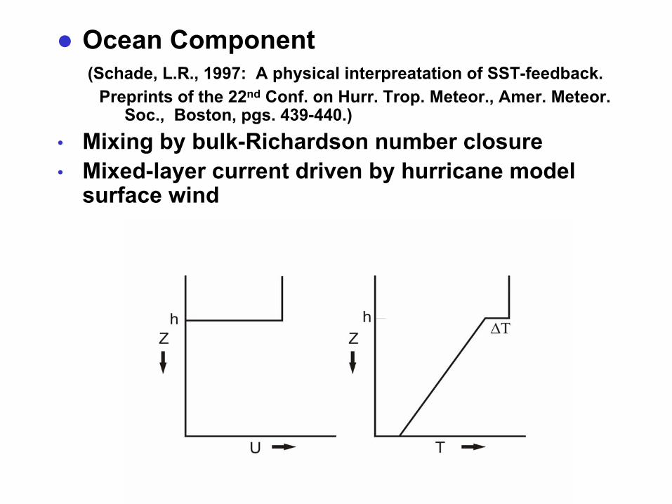
z Ocean Component (Schade, L.R., 1997: A physical interpreatation of SST-feedback.
Preprints of the 22nd Conf. on Hurr. Trop. Meteor., Amer. Meteor. Soc., Boston, pgs. 439-440.)
• Mixing by bulk-Richardson number closure • Mixed-layer current driven by hurricane model
surface wind

Ocean columns integrated only Along predicted storm track. Predicted storm center SST anomaly used for input to ALL atmospheric points.

zData Inputs: –Weekly updated potentialintensity (1 X 1 degree) –Official track forecast and storm history (NHC &JTWC) –Monthly climatologicalocean mixed layer depths(1 X 1 degree) –Monthly climatologicalsub-mixed layer thermalstratification (1 X 1 degree) –Bathymetry (1/4 X 1/4degree)

Initialization:
• Synthetic, warm core vortex specified at beginning of track
• Radial eddy flux of entropy at middle levels adjusted so as to match storm intensity to date
• This matching procedure effectively initializes middle tropospheric humidity as well as balanced flow

Comparison with same atmospheric model coupled to 3-D ocean model; idealized runs:
Full model (black), string model (red)
Courtesy of Robert Korty. Used with permission.

Mixed layer depth and currents
Courtesy of Robert Korty. Used with permission.

Courtesy of Robert Korty. Used with permission.

SST Change
Courtesy of Robert Korty. Used with permission.

Courtesy of Robert Korty. Used with permission.

Courtesy of Robert Korty. Used with permission.

Landfall Algorithm:
• Enthalpy exchange coefficient decreases linearly with land elevation, reaching zero when h = 40 m
• This accounts in a crude way for heat fluxes from low-lying, swampy or marshy terrain

Real-Time Forecasts Posted at http://wind.mit.edu/~emanuel/storm.html
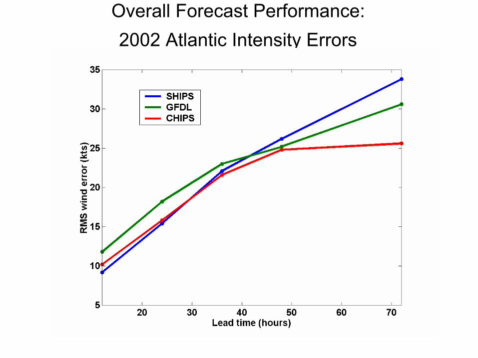
Overall Forecast Performance: 2002 Atlantic Intensity Errors

70
Hurricane Gert occurred in a low-shear environment and moved over an ocean close to its climatological mean state.
Gert, 1999 M
axim
um s
urfa
ce w
ind
spee
d (m
/s)
60
50
40
30
20
10 12 14 16 18 20 22 24
Observed Model Initialization period
September

Same simulation, but with fixed SST:

Sensitivity to initial intensity error and length of matching period:

Sensitivity to size of starting vortex

Model performs poorly when substantial shear is present, as in Chantal, 2001:
Chantal, 2001 M
axim
um s
urfa
ce w
ind
spee
d (m
s-1
) 70
60
50
40
30
20
10
0
Best track Model
Initialization period
16 17 18 19 20 21 22 23 24 August
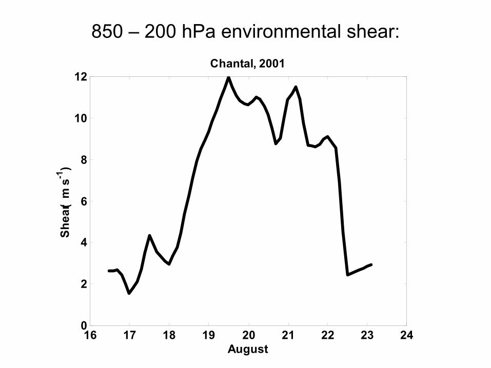
850 – 200 hPa environmental shear:
12
(-1
)
10
8
6
4
2
0
Chantal, 2001Sh
ear
m s
16 17 18 19 20 21 22 23 24 August

Add “ventilation” term to model equation governing middle level θe. Coefficient determined by matching model to long
record of observations:
∂θ e = … − V (θ −θ e e0 )∂t
V = V 2 V 2 max shear
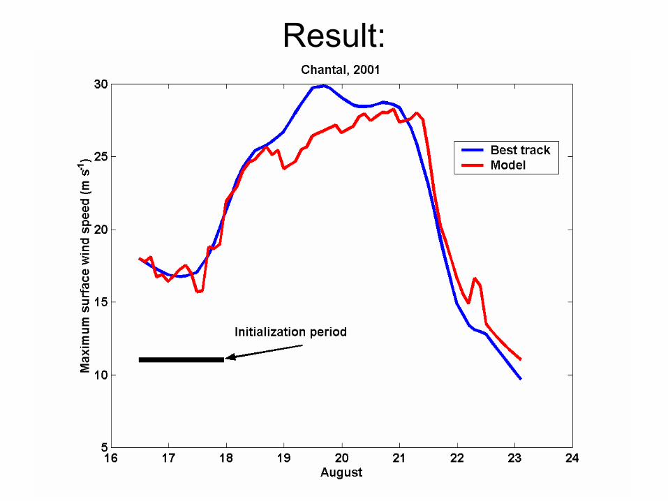
Result:

But model sensitive to shear: This shows the results of varying Shear magnitude by +/- 5 kts and +/- 10 kts:

Presence of shear also makes model sensitive to initial conditions. Here the initial intensity is varied by +/- 3 m/s and +/- 6 m/s:

Some storms are influenced by upper ocean anomalies from monthly climatology. An example is that of Typhoon Maemi of 2003, which passed over a warm eddy in the western North Pacific:
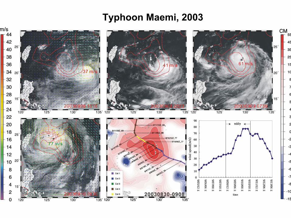
Typhoon Maemi, 2003


upper-layer
lower
upperlowergg ρ
ρρ − =′
200C isotherm
upperρ
lowerρ
η′
η
~500km
lower-layer

Standard Simulation:
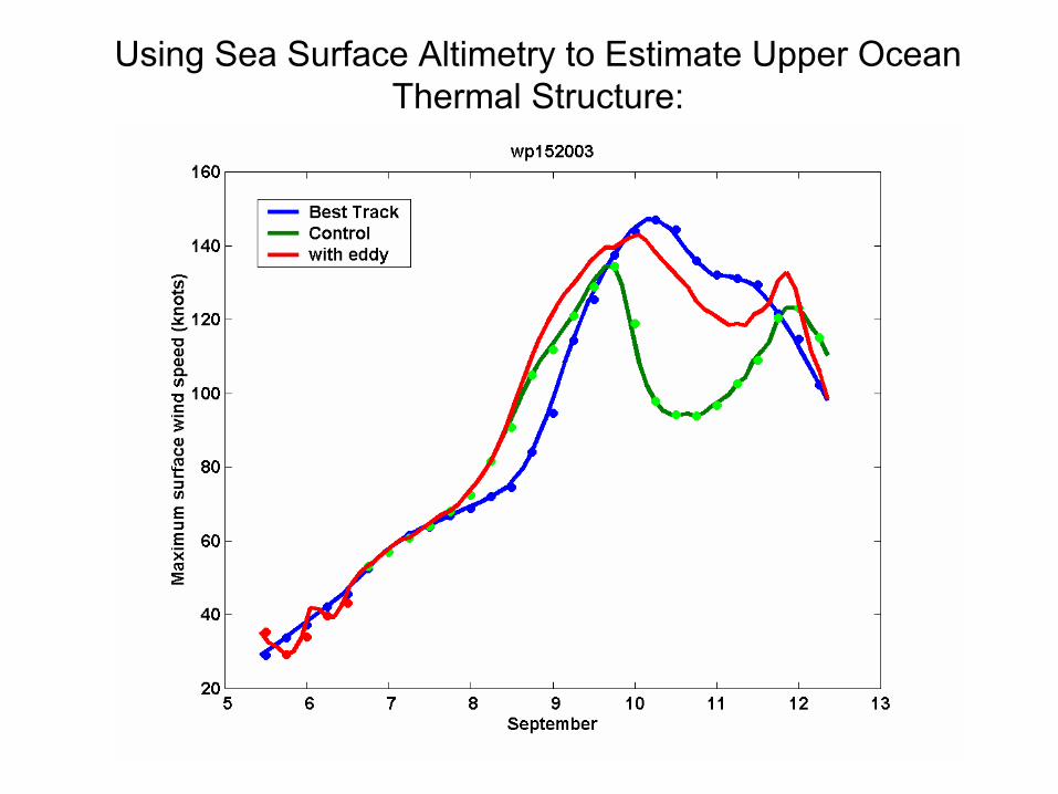
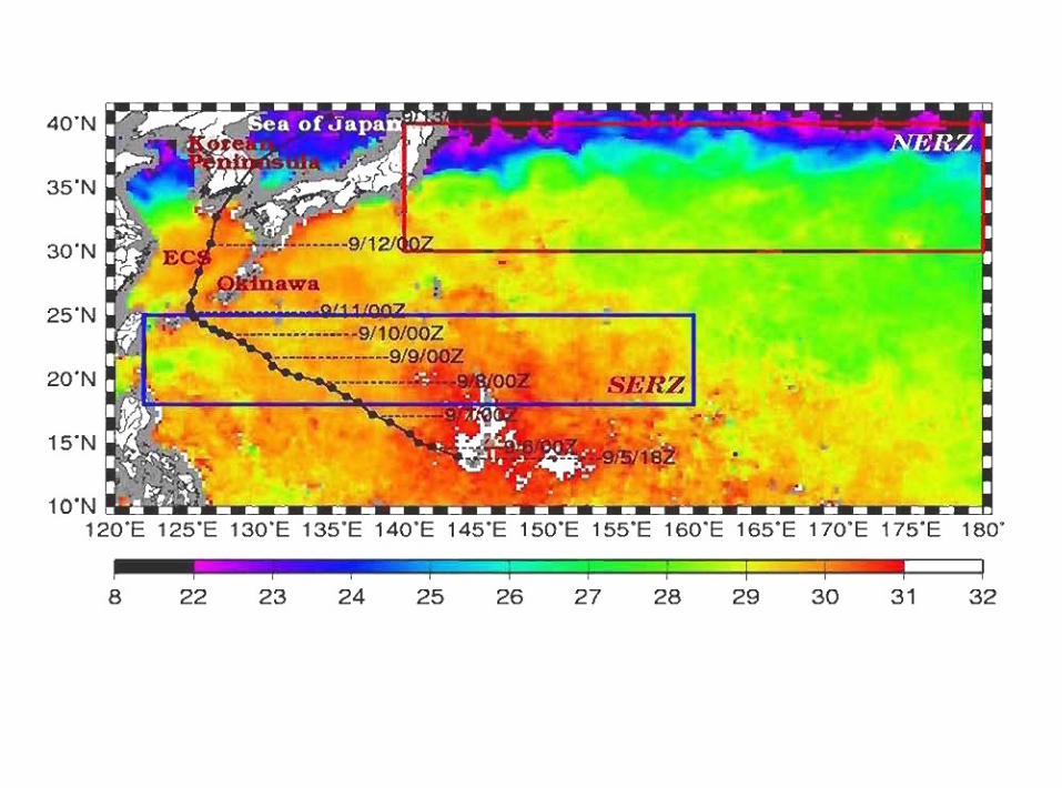
Using Sea Surface Altimetry to Estimate Upper Ocean Thermal Structure:
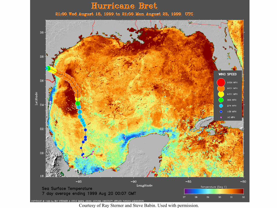
Courtesy of Ray Sterner and Steve Babin. Used with permission.

This shows model hindcasts with and without the ocean eddy, as estimated from sea surface altimetry data:

As TCs approach shore, shoaling water isolates surface mixed layer... surface cooling ceases.


A good simulation of Camille can only be obtained by assuming that it traveled right up the axis of the Loop Current:

Mitch was also influenced by an ocean eddy. The red curve used TOPEX altimetry modified by de-aliasing the estimated peak amplitude:

Effect of standing water can be seen in these idealized simulations of storm landfall over dry land and over swamps with indicated depths of standing water:

Hurricane Andrew, with and without the effect of the Everglades, as represented by a elevation-dependent heat exchange coefficient:

Some storms may have large internal fluctuations (e.g. Allen). CHIPS may predict the existence of these, but not their phase:

Concentric eyewalls in Hurricane Gilbert, 1988 (from Black and Willoughby, Mon. Wea. Rev., 1992)
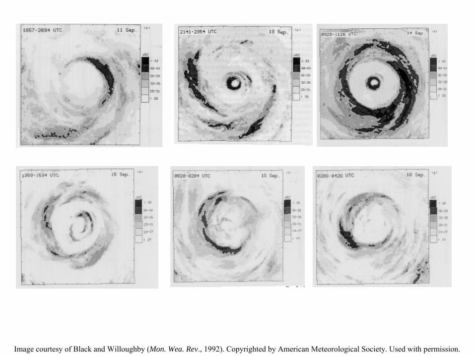
Image courtesy of Black and Willoughby (Mon. Wea. Rev., 1992). Copyrighted by American Meteorological Society. Used with permission.
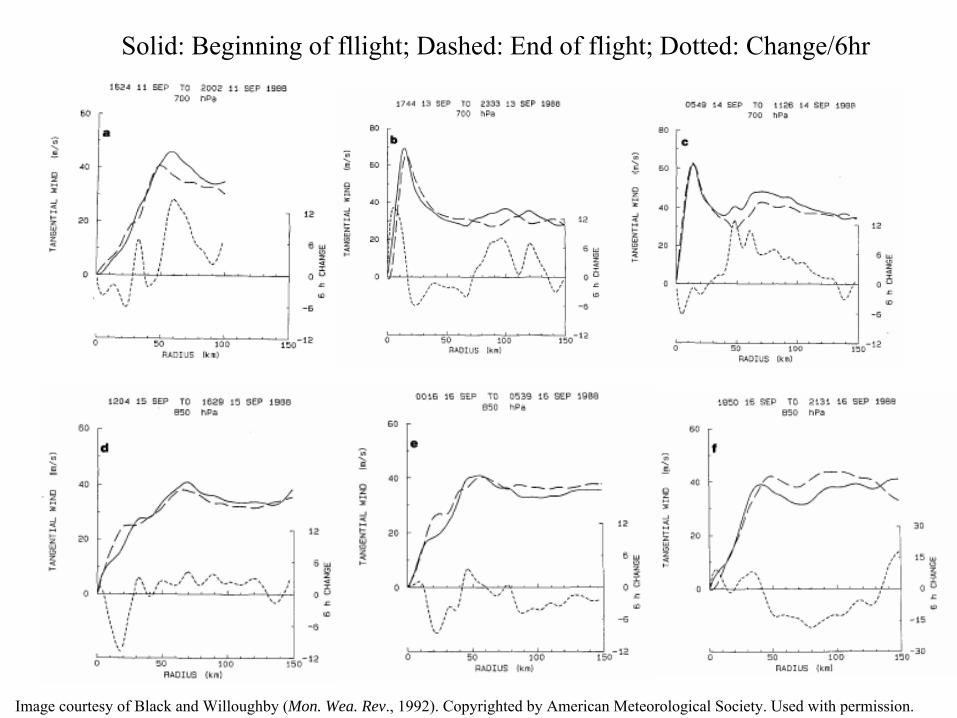
Image courtesy of Black and Willoughby (Mon. Wea. Rev., 1992). Copyrighted by American Meteorological Society. Used with permission.
Solid: Beginning of fllight; Dashed: End of flight; Dotted: Change/6hr

Image courtesy of Black and Willoughby (Mon. Wea. Rev., 1992). Copyrighted by American Meteorological Society. Used with permission.

Image courtesy of Black and Willoughby (Mon. Wea. Rev., 1992). Copyrighted by American Meteorological Society. Used with permission.

Environmental factors critical to intensity prediction:
• Potential intensity along track • Upper ocean thermal structure • Environmental wind shear • Bathymetry • Land surface characteristics

Major sources of uncertainty:
• Uncertain forecasts of vertical shear • Shear reduces predictability • Little real-time knowledge of upper
ocean thermal structure • Low predictability of internal variability

Hurricanes and Climate

150
160
170
180
190
200
210
220
230
240 (
)M
axim
um W
ind
Spee
d M
PH
80 82 84 86 88 90 92 94 Sea Surface Temperature (F)
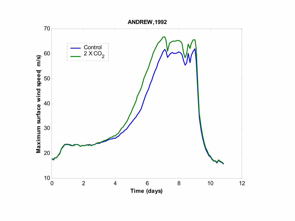
70 ANDREW,1992
60
50
40
30
20
10 0 2 4 6 8 10 12
(m
/s) 2
Max
imum
sur
face
win
d sp
eed
Control 2 X CO
Time (days)

Empirical Index: 3
3 − 25I = 10 η 2 H
3 V
pot 1 0.1 V , 50 70
+ shear
(η ≡ 850 hPa absolute vorticity s − 1),
Vpot ≡ Potential wind speed (ms− 1),
H ≡ 600 mb relative humidity (%),
V ≡ V − V (ms − 1).shear 850 250
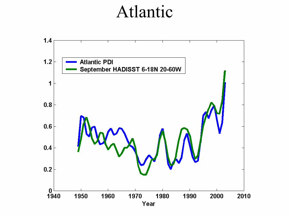
Atlantic

Western North Pacific

Paleotempestology
Courtesy of The Geological Society of America. Used with permission.
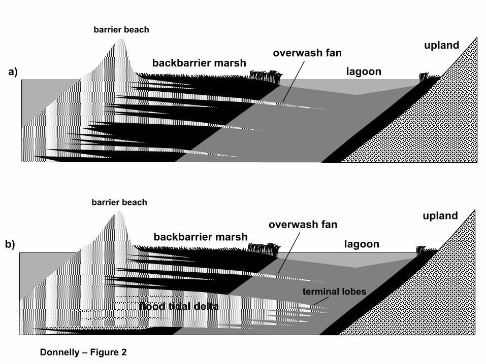
barrier beach
a)
b)
lagoon
barrier beach
lagoon
upland
upland
flood tidal delta
overwash fan
overwash fan backbarrier marsh
backbarrier marsh
terminal lobes
Donnelly – Figure 2

0
Pearl River Marsh
Pascagoula MarshLake Shelby
500
1,000
1,500
2,000
4,500
4,000
3,500
3,000
14
2,500
Western Lake C
Age
(Yea
rs B
efor
e Pr
esen
t)
Figure by MIT OCW.

Whale Beach
WB1 WB2 WB3 0
50
100
150
200
250
300
350
fine sand
mud with S. alterniflora
salt marsh peat
Dep
th (c
m)
? ?
1962 nor’easter
late 1700s or early 1800s
1278-1434 A.D.
pre-1932
50) 1301-1370 A.D. 1376-1434 A.D.
30) 1278-1319 A.D. 1353-1389 A.D.
probably 1821 Hurricane
(560 +
(680 +
Jeffrey Donnelly, WHOI
Courtesy of Jeffrey Donnelly. Used with permission.

Gulf of Carpentaria
Is.
Cairns
Great Barrier Reef
BEACH DEPOSITS
Princess Charlotte Bay
Fitzroy Is.
Norman by Is.
Lady Elliot Is.
Curacoa Is.
300 km
Wallaby
Red Cliff
N E Australia
Figure by MIT OCW.
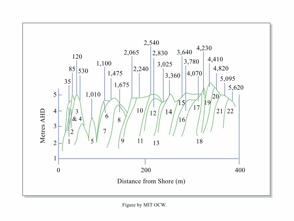
Distance from Shore (m)
1
2
3
4
5
0
1 2
3 & 4
5 7
6 8
9
10 12
13
14 15
16
17
18
20 19
35
85
120
530
1,010
1,100 1,475
1,675
2,065
2,240
2,540 2,830
3,025
3,360
3,640 4,230
5,620 5,095
4,820 4,4103,780
4,070
200 400
11
22 21
Met
res A
HD
Figure by MIT OCW.

0 400 Distance from Shore (m)
Supra-tidal mudflats KEY
800
0
1
2
3
1
70 300 465 565
785 1,060
1,190
1,360 1,730
1,930
1,965 2,525
2
3 4 5 7
8
9
10
126
Met
res A
HD
11
Figure by MIT OCW.

7 N
umbe
r of e
vent
s
6
5
4
3
2
1
0 250 750 1250 1750 2250 2750
Years before present

Lake Inwash Deposits Noren et al., 2002

Hummocky Cross-StratificationDuke, 1985
X (M)
F H
P B
Low-Angle Truncations and Terminations Low-Angle Curved Laminae, Both Concave- and
Convex-Upward
About 1m.
Sharp base
Directional sole marks
Upward growth of Hummocks from parallel lamination
Figure by MIT OCW.

Figure by MIT OCW.
00 20
Degrees Paleolatitude
Occ
urre
nces
of H
.C.S
.
40 60 80
2
4
6
8
10
00 20
Degrees Paleolatitude
Occ
urre
nces
of H
.C.S
.
40 60 80
2
4
6
8
10
00 20
Degrees Paleolatitude
Occ
urre
nces
of H
.C.S
.
40 60 80
2
4
6
8
10
00 20
Degrees Paleolatitude
Occ
urre
nces
of H
.C.S
.
40 60 80
2
4
6
8
10
Neogene and Quaternaryn = 15
Group A Mean = 31*Group B Mean = 42*
Mesozoic and Paleogenen = 33
Group A Mean = 40*Group B Mean = 52*
Proterozoic and Paleozoicn = 47
Group A Mean = 17*Group B Mean = 58*
Proterozoic, Paleozoic, Neogene and Quaternary
n = 62Group A Mean = 19*Group B Mean = 49*

Brandt and Elias, 1989
Courtesy of The Geological Society of America. Used with permission.

Do tropical cyclones play a role in the climate system?
••The case for tropical cyclone controlThe case for tropical cyclone control of the thermohaline circulationof the thermohaline circulation
••Feedback of tropical cyclone activityFeedback of tropical cyclone activity on climateon climate

Tropical Cyclone-Climate Feedback
• Sensitive dependence of tropical cyclone frequency and intensity on tropical SSTs
+ • Dependence of tropical SSTs on global
tropical cyclone activity
= Tropical thermostat

Ocean Feedback
Ocean Thermohaline Circulation
Image removed due to copyright considerations.
Source: Broocker, 1991, in Climate change 1995, impacts, adaptations and mitigation of climate change: scientific-technical analysis, contribution of working group 2 to the second assessment report of the intergovernmental panel on climate change, UNEP and WMO, Cambridge press university, 1996.

-90 -6
-4
-2
0
2
4
6
-60 -30 Latitude
0 30 60 90
Atmosphere
Heat Transport by Oceans and Atmosphere
peta
Wat
ts
Ocean Transport
Total Transport Transport
Figure by MIT OCW.

A hot plate is brought in contact with the left half of the surface of a swimming pool of cold water. Heat diffuses downward and the warm water begins to rise. The strength of the circulation is controlled in part by the rate of heat diffusion. In the real world, this rate is very, very small.
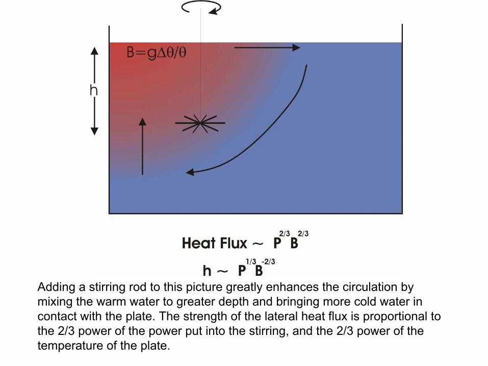
Adding a stirring rod to this picture greatly enhances the circulation by mixing the warm water to greater depth and bringing more cold water in contact with the plate. The strength of the lateral heat flux is proportional to the 2/3 power of the power put into the stirring, and the 2/3 power of the temperature of the plate.

Coupled Ocean-Atmosphere model run for 67 of the 83 tropical cyclones that occurred in calendar year 1996
Accumulated TC-induced ocean heating divided by 366 days
Result:
Net column-integrated heating of ocean induced by global tropical cyclone activity:
(1.4 0.7 )×1015 W±


Veronique Bugnion used an ocean model to calculate the sensitivity of the total poleward heat flux by the world oceans to the strength and distribution of vertical mixing. This sensitivity, shown here, is concentrated in the Tropics, where hurricanes occur.
Image courtesy of Véronique Bugnion. Used with permission.
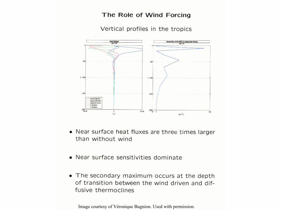
Image courtesy of Véronique Bugnion. Used with permission.

These diagrams show the currents generated by a very localized source of vertical mixing at 20o N and 25o E. The upper diagram shows the currents near the top of the ocean, while the bottom diagram show currents closer to the bottom. Note in particular the strong northward flow of warm water along the western boundary of the ocean, near the surface. These plots have been generated using a complex ocean model set in a simple rectangular basin.
Image by Jeff Scott. © Copyright 2006 American Meteorological Society (AMS). Used with permission of AMS.

Implications for Climate: 2
∼ FP 3Poleward Heat Flux
F PI 3∼
P ∼ PI3
→Poleward Heat Flux ∼ PI 5
May be conservative, in view of Nolan’s results

This plot shows a measure of El Niño/La Niña (green) and a measure of the power put into the far western Pacific Ocean by tropical cyclones (blue). The blue curve has been shifted rightward by two years on this graph. There is the suggestion that powerful cyclones in the western Pacific can trigger El Niño/La Niña cycles.

90S -5
0
5
10
15
20
25
30
45S
Modern (red line) and estimated early Eocene (purple lines) zonal sea surface temperatures. Modern (light blue) and estimated early Eocene (dark blue) water temperatures at bottom depths between 1000m and 5000m.
0 45N
? ?
90N Latitude
o C)
Tem
pera
ture
(
Figure by MIT OCW.
Top Related