


Languages
Pages
Legal

Compute R0 Using Next Generation Operator
Baojun Song, Ph.D.
Department of Mathematical SciencesMontclair State University
June 20, 2016
B. Song (Montclair State) Compute R0 June 20, 2016 1 / 1

Compute R0 Using Next Generation Operator
Reference: P. van den Driessche and J.
Watmough (2002). Reproduction numbers and
sub-threshold endemic equilibria for
compartmental models of disease transmission,
Mathematical Biosciences, 180:29–48
B. Song (Montclair State) Compute R0 June 20, 2016 2 / 1

Definition and a Theorem
Basic reproductive number (R0) is defined as the average number ofsecondary infections when a typical infective enters an entirelysusceptible population.
Theorem
If R0 < 1, then DFE (disease-free equilibrium) islocally asymptotically stable(L.A.S.). If R0 > 1, thenDFE is unstable.
If you compute R0, you need not prove the stability of DFE.
B. Song (Montclair State) Compute R0 June 20, 2016 3 / 1

Two Types of Epidemiological Classes
• Let X be vector of infected classes, such asexposed, infectious, carrier, etc.
• Let Y be vector of uninfected classes, such assusceptible, recovered, etc.
B. Song (Montclair State) Compute R0 June 20, 2016 4 / 1

Two Types of Epidemiological Classes
• Let X be vector of infected classes, such asexposed, infectious, carrier, etc.
• Let Y be vector of uninfected classes, such assusceptible, recovered, etc.
B. Song (Montclair State) Compute R0 June 20, 2016 4 / 1
Rearrange System of Equations
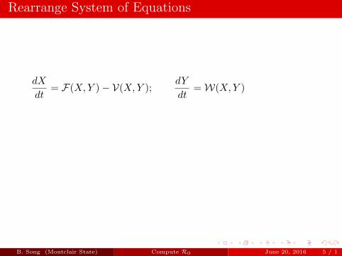
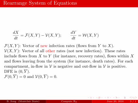
dX
dt= F(X,Y )− V(X,Y );
dY
dt=W(X,Y )
F(X,Y ): Vector of new infection rates (flows from Y to X).V(X,Y ): Vector of all other rates (not new infection). These ratesinclude flows from X to Y (for instance, recovery rates), flows within Xand flows leaving from the system (for instance, death rates). For eachcompartment, in-flow in V is negative and out-flow in V is positive.DFE is (0, Y ).F(0, Y ) = 0 and V(0, Y ) = 0.
B. Song (Montclair State) Compute R0 June 20, 2016 5 / 1

Rearrange System of Equations
dX
dt= F(X,Y )− V(X,Y );
dY
dt=W(X,Y )
F(X,Y ): Vector of new infection rates (flows from Y to X).
V(X,Y ): Vector of all other rates (not new infection). These ratesinclude flows from X to Y (for instance, recovery rates), flows within Xand flows leaving from the system (for instance, death rates). For eachcompartment, in-flow in V is negative and out-flow in V is positive.DFE is (0, Y ).F(0, Y ) = 0 and V(0, Y ) = 0.
B. Song (Montclair State) Compute R0 June 20, 2016 5 / 1

Rearrange System of Equations
dX
dt= F(X,Y )− V(X,Y );
dY
dt=W(X,Y )
F(X,Y ): Vector of new infection rates (flows from Y to X).V(X,Y ): Vector of all other rates (not new infection). These ratesinclude flows from X to Y (for instance, recovery rates), flows within Xand flows leaving from the system (for instance, death rates). For eachcompartment, in-flow in V is negative and out-flow in V is positive.
DFE is (0, Y ).F(0, Y ) = 0 and V(0, Y ) = 0.
B. Song (Montclair State) Compute R0 June 20, 2016 5 / 1

Rearrange System of Equations
dX
dt= F(X,Y )− V(X,Y );
dY
dt=W(X,Y )
F(X,Y ): Vector of new infection rates (flows from Y to X).V(X,Y ): Vector of all other rates (not new infection). These ratesinclude flows from X to Y (for instance, recovery rates), flows within Xand flows leaving from the system (for instance, death rates). For eachcompartment, in-flow in V is negative and out-flow in V is positive.DFE is (0, Y ).
F(0, Y ) = 0 and V(0, Y ) = 0.
B. Song (Montclair State) Compute R0 June 20, 2016 5 / 1
Rearrange System of Equations
dX
dt= F(X,Y )− V(X,Y );
dY
dt=W(X,Y )
F(X,Y ): Vector of new infection rates (flows from Y to X).V(X,Y ): Vector of all other rates (not new infection). These ratesinclude flows from X to Y (for instance, recovery rates), flows within Xand flows leaving from the system (for instance, death rates). For eachcompartment, in-flow in V is negative and out-flow in V is positive.DFE is (0, Y ).F(0, Y ) = 0 and V(0, Y ) = 0.
B. Song (Montclair State) Compute R0 June 20, 2016 5 / 1

Jacobian around DFE
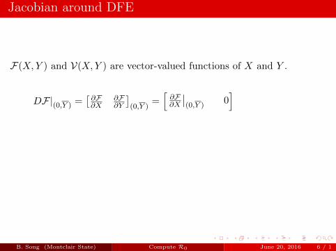
F(X,Y ) and V(X,Y ) are vector-valued functions of X and Y .
DF|(0,Y ) =[∂F∂X
∂F∂Y
](0,Y )
=[∂F∂X
∣∣(0,Y )
0]
DV|(0,Y ) =[∂V∂X
∂V∂Y
](0,Y )
=[∂V∂X
∣∣(0,Y )
0]
B. Song (Montclair State) Compute R0 June 20, 2016 6 / 1
Jacobian around DFE
F(X,Y ) and V(X,Y ) are vector-valued functions of X and Y .
DF|(0,Y ) =[∂F∂X
∂F∂Y
](0,Y )
=[∂F∂X
∣∣(0,Y )
0]
DV|(0,Y ) =[∂V∂X
∂V∂Y
](0,Y )
=[∂V∂X
∣∣(0,Y )
0]
B. Song (Montclair State) Compute R0 June 20, 2016 6 / 1

Jacobian around DFE
F(X,Y ) and V(X,Y ) are vector-valued functions of X and Y .
DF|(0,Y ) =[∂F∂X
∂F∂Y
](0,Y )
=[∂F∂X
∣∣(0,Y )
0]
DV|(0,Y ) =[∂V∂X
∂V∂Y
](0,Y )
=[∂V∂X
∣∣(0,Y )
0]
B. Song (Montclair State) Compute R0 June 20, 2016 6 / 1

Formula for R0
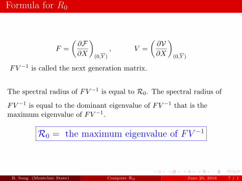
F =
(∂F∂X
)(0,Y )
, V =
(∂V∂X
)(0,Y )
FV −1 is called the next generation matrix.
The spectral radius of FV −1 is equal to R0. The spectral radius of
FV −1 is equal to the dominant eigenvalue of FV −1 that is themaximum eigenvalue of FV −1.
R0 = the maximum eigenvalue of FV −1
B. Song (Montclair State) Compute R0 June 20, 2016 7 / 1

Formula for R0
F =
(∂F∂X
)(0,Y )
, V =
(∂V∂X
)(0,Y )
FV −1 is called the next generation matrix.
The spectral radius of FV −1 is equal to R0.
The spectral radius of
FV −1 is equal to the dominant eigenvalue of FV −1 that is themaximum eigenvalue of FV −1.
R0 = the maximum eigenvalue of FV −1
B. Song (Montclair State) Compute R0 June 20, 2016 7 / 1

Formula for R0
F =
(∂F∂X
)(0,Y )
, V =
(∂V∂X
)(0,Y )
FV −1 is called the next generation matrix.
The spectral radius of FV −1 is equal to R0. The spectral radius of
FV −1 is equal to the dominant eigenvalue of FV −1 that is themaximum eigenvalue of FV −1.
R0 = the maximum eigenvalue of FV −1
B. Song (Montclair State) Compute R0 June 20, 2016 7 / 1

Example 1: An SIR Model
Model Equations
dS
dt= Λ− βS I
N− µS,
dI
dt= βS
I
N− (µ+ γ)I,
dR
dt= γI − µR,
N = S + I +R.
DFE: (0,Λ/µ, 0)
F =
(∂F∂I
)∣∣∣∣(0,Λ/µ,0)
= β, V =
(∂V∂I
)∣∣∣∣(0,Λ/µ,0)
= µ+ γ
B. Song (Montclair State) Compute R0 June 20, 2016 8 / 1

Example 1: An SIR Model
Model Equations
dS
dt= Λ− βS I
N− µS,
dI
dt= βS
I
N− (µ+ γ)I,
dR
dt= γI − µR,
N = S + I +R.
Rearrange
X = I, Y = [S,R]T
F(I) = βSI
N,
V(I, S,R) = (µ+ γ)I
dI
dt= F(I)− V(I, S,R)
DFE: (0,Λ/µ, 0)
F =
(∂F∂I
)∣∣∣∣(0,Λ/µ,0)
= β, V =
(∂V∂I
)∣∣∣∣(0,Λ/µ,0)
= µ+ γ
B. Song (Montclair State) Compute R0 June 20, 2016 8 / 1

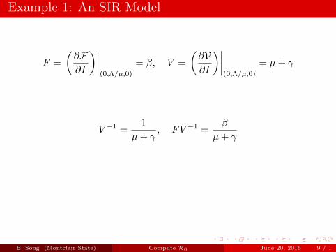
Example 1: An SIR Model
F =
(∂F∂I
)∣∣∣∣(0,Λ/µ,0)
= β, V =
(∂V∂I
)∣∣∣∣(0,Λ/µ,0)
= µ+ γ
V −1 =1
µ+ γ, FV −1 =
β
µ+ γ
R0 =β
µ+ γ
B. Song (Montclair State) Compute R0 June 20, 2016 9 / 1
Example 1: An SIR Model
F =
(∂F∂I
)∣∣∣∣(0,Λ/µ,0)
= β, V =
(∂V∂I
)∣∣∣∣(0,Λ/µ,0)
= µ+ γ
V −1 =1
µ+ γ, FV −1 =
β
µ+ γ
R0 =β
µ+ γ
B. Song (Montclair State) Compute R0 June 20, 2016 9 / 1

Example 1: An SIR Model
F =
(∂F∂I
)∣∣∣∣(0,Λ/µ,0)
= β, V =
(∂V∂I
)∣∣∣∣(0,Λ/µ,0)
= µ+ γ
V −1 =1
µ+ γ, FV −1 =
β
µ+ γ
R0 =β
µ+ γ
B. Song (Montclair State) Compute R0 June 20, 2016 9 / 1

Example 2: An SEIR Model
Model Equations
dS
dt= Λ− βS I
N− µS,
dE
dt= βS
I
N− (µ+ k + r1)E,
dI
dt= kE − (γ + µ)I,
dR
dt= r1E + γI − µR.
Rearrange Equations
X =
[EI
], Y =
[SR
]F =
[βS I
N0
]V =
[(µ+ k + r1)E−kE + (γ + µ)I
]
DFE: (0, 0,Λ/µ, 0)
B. Song (Montclair State) Compute R0 June 20, 2016 10 / 1

Example 2: An SEIR Model
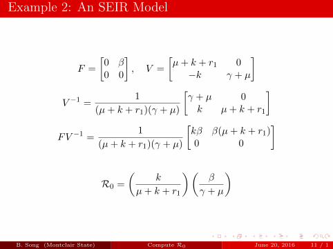
F =
[0 β0 0
], V =
[µ+ k + r1 0−k γ + µ
]
V −1 =1
(µ+ k + r1)(γ + µ)
[γ + µ 0k µ+ k + r1
]
FV −1 =1
(µ+ k + r1)(γ + µ)
[kβ β(µ+ k + r1)0 0
]
R0 =
(k
µ+ k + r1
)(β
γ + µ
)
B. Song (Montclair State) Compute R0 June 20, 2016 11 / 1

Example 2: An SEIR Model
F =
[0 β0 0
], V =
[µ+ k + r1 0−k γ + µ
]
V −1 =1
(µ+ k + r1)(γ + µ)
[γ + µ 0k µ+ k + r1
]
FV −1 =1
(µ+ k + r1)(γ + µ)
[kβ β(µ+ k + r1)0 0
]
R0 =
(k
µ+ k + r1
)(β
γ + µ
)
B. Song (Montclair State) Compute R0 June 20, 2016 11 / 1

Example 2: An SEIR Model
F =
[0 β0 0
], V =
[µ+ k + r1 0−k γ + µ
]
V −1 =1
(µ+ k + r1)(γ + µ)
[γ + µ 0k µ+ k + r1
]
FV −1 =1
(µ+ k + r1)(γ + µ)
[kβ β(µ+ k + r1)0 0
]
R0 =
(k
µ+ k + r1
)(β
γ + µ
)
B. Song (Montclair State) Compute R0 June 20, 2016 11 / 1
Example 2: An SEIR Model
F =
[0 β0 0
], V =
[µ+ k + r1 0−k γ + µ
]
V −1 =1
(µ+ k + r1)(γ + µ)
[γ + µ 0k µ+ k + r1
]
FV −1 =1
(µ+ k + r1)(γ + µ)
[kβ β(µ+ k + r1)0 0
]
R0 =
(k
µ+ k + r1
)(β
γ + µ
)
B. Song (Montclair State) Compute R0 June 20, 2016 11 / 1
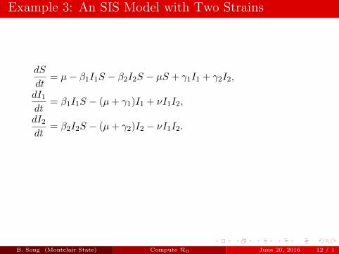
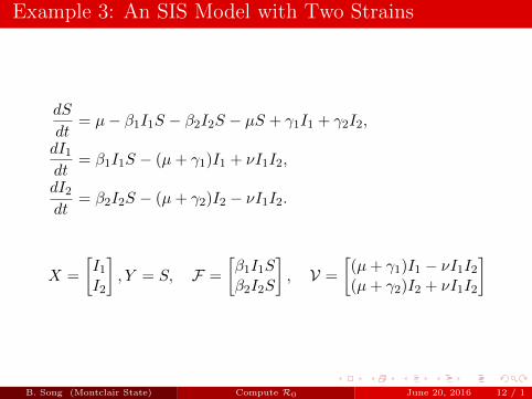
Example 3: An SIS Model with Two Strains
dS
dt= µ− β1I1S − β2I2S − µS + γ1I1 + γ2I2,
dI1
dt= β1I1S − (µ+ γ1)I1 + νI1I2,
dI2
dt= β2I2S − (µ+ γ2)I2 − νI1I2.
X =
[I1
I2
], Y = S, F =
[β1I1Sβ2I2S
], V =
[(µ+ γ1)I1 − νI1I2
(µ+ γ2)I2 + νI1I2
]DFE: (0, 0, 1)
B. Song (Montclair State) Compute R0 June 20, 2016 12 / 1
Example 3: An SIS Model with Two Strains
dS
dt= µ− β1I1S − β2I2S − µS + γ1I1 + γ2I2,
dI1
dt= β1I1S − (µ+ γ1)I1 + νI1I2,
dI2
dt= β2I2S − (µ+ γ2)I2 − νI1I2.
X =
[I1
I2
], Y = S, F =
[β1I1Sβ2I2S
], V =
[(µ+ γ1)I1 − νI1I2
(µ+ γ2)I2 + νI1I2
]
DFE: (0, 0, 1)
B. Song (Montclair State) Compute R0 June 20, 2016 12 / 1

Example 3: An SIS Model with Two Strains
dS
dt= µ− β1I1S − β2I2S − µS + γ1I1 + γ2I2,
dI1
dt= β1I1S − (µ+ γ1)I1 + νI1I2,
dI2
dt= β2I2S − (µ+ γ2)I2 − νI1I2.
X =
[I1
I2
], Y = S, F =
[β1I1Sβ2I2S
], V =
[(µ+ γ1)I1 − νI1I2
(µ+ γ2)I2 + νI1I2
]DFE: (0, 0, 1)
B. Song (Montclair State) Compute R0 June 20, 2016 12 / 1

Example 3: An SIS Model with Two Strains
F =
[f1
f2
]=
[β1I1Sβ2I2S
], V =
[v1
v2
]=
[(µ+ γ1)I1 − νI1I2
(µ+ γ2)I2 + νI1I2
]
F =
[∂f1∂I1
∂f1∂I2
∂f2∂I1
∂f2∂I2
](0,0,1)
=
[β1 00 β2
]
V =
[∂v1∂I1
∂v1∂I2
∂v2∂I1
∂v2∂I2
](0,0,1)
=
[µ+ γ1 0
0 µ+ γ2
], V −1 =
[1
µ+γ10
0 1µ+γ2
]
B. Song (Montclair State) Compute R0 June 20, 2016 13 / 1

Example 3: An SIS Model with Two Strains
F =
[β1 00 β2
], V −1 =
[1
µ+γ10
0 1µ+γ2
]
FV −1 =
[β1 00 β2
] [ 1µ+γ1
0
0 1µ+γ2
]=
[β1
µ+γ10
0 β2µ+γ2
]
R0 = max
{β1
µ+ γ1,
β2
µ+ γ2
}
B. Song (Montclair State) Compute R0 June 20, 2016 14 / 1

Example 3: An SIS Model with Two Strains
F =
[β1 00 β2
], V −1 =
[1
µ+γ10
0 1µ+γ2
]
FV −1 =
[β1 00 β2
] [ 1µ+γ1
0
0 1µ+γ2
]=
[β1
µ+γ10
0 β2µ+γ2
]
R0 = max
{β1
µ+ γ1,
β2
µ+ γ2
}
B. Song (Montclair State) Compute R0 June 20, 2016 14 / 1

Example 3: An SIS Model with Two Strains
F =
[β1 00 β2
], V −1 =
[1
µ+γ10
0 1µ+γ2
]
FV −1 =
[β1 00 β2
] [ 1µ+γ1
0
0 1µ+γ2
]=
[β1
µ+γ10
0 β2µ+γ2
]
R0 = max
{β1
µ+ γ1,
β2
µ+ γ2
}
B. Song (Montclair State) Compute R0 June 20, 2016 14 / 1
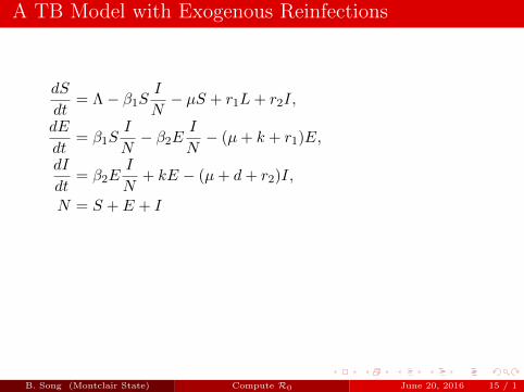
A TB Model with Exogenous Reinfections
dS
dt= Λ− β1S
I
N− µS + r1L+ r2I,
dE
dt= β1S
I
N− β2E
I
N− (µ+ k + r1)E,
dI
dt= β2E
I
N+ kE − (µ+ d+ r2)I,
N = S + E + I
X =
[EI
], Y = [S]
F =
[β1S
IN
0
], V =
[(µ+ k + r1)E + β2E
IN
−kE + (µ+ d+ r2)I − β2EIN
]
B. Song (Montclair State) Compute R0 June 20, 2016 15 / 1

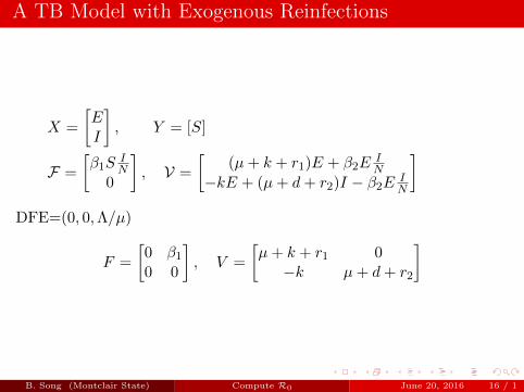
A TB Model with Exogenous Reinfections
X =
[EI
], Y = [S]
F =
[β1S
IN
0
], V =
[(µ+ k + r1)E + β2E
IN
−kE + (µ+ d+ r2)I − β2EIN
]DFE=(0, 0,Λ/µ)
F =
[0 β1
0 0
], V =
[µ+ k + r1 0−k µ+ d+ r2
]
B. Song (Montclair State) Compute R0 June 20, 2016 16 / 1
A TB Model with Exogenous Reinfections
X =
[EI
], Y = [S]
F =
[β1S
IN
0
], V =
[(µ+ k + r1)E + β2E
IN
−kE + (µ+ d+ r2)I − β2EIN
]DFE=(0, 0,Λ/µ)
F =
[0 β1
0 0
], V =
[µ+ k + r1 0−k µ+ d+ r2
]
B. Song (Montclair State) Compute R0 June 20, 2016 16 / 1

A TB Model with Exogenous Reinfections
F =
[0 β1
0 0
], V =
[µ+ k + r1 0−k µ+ d+ r2
]
V −1 =1
(µ+ k + r1)(µ+ d+ r2)
[µ+ d+ r2 0
k µ+ k + r1
]
FV −1 =1
(µ+ k + r1)(µ+ d+ r2)
[kβ1 β1(µ+ k + r1)0 0
]
R0 =
(β1
µ+ d+ r2
)(k
µ+ k + r1
)
B. Song (Montclair State) Compute R0 June 20, 2016 17 / 1

A TB Model with Exogenous Reinfections
F =
[0 β1
0 0
], V =
[µ+ k + r1 0−k µ+ d+ r2
]
V −1 =1
(µ+ k + r1)(µ+ d+ r2)
[µ+ d+ r2 0
k µ+ k + r1
]
FV −1 =1
(µ+ k + r1)(µ+ d+ r2)
[kβ1 β1(µ+ k + r1)0 0
]
R0 =
(β1
µ+ d+ r2
)(k
µ+ k + r1
)
B. Song (Montclair State) Compute R0 June 20, 2016 17 / 1

A TB Model with Exogenous Reinfections
F =
[0 β1
0 0
], V =
[µ+ k + r1 0−k µ+ d+ r2
]
V −1 =1
(µ+ k + r1)(µ+ d+ r2)
[µ+ d+ r2 0
k µ+ k + r1
]
FV −1 =1
(µ+ k + r1)(µ+ d+ r2)
[kβ1 β1(µ+ k + r1)0 0
]
R0 =
(β1
µ+ d+ r2
)(k
µ+ k + r1
)
B. Song (Montclair State) Compute R0 June 20, 2016 17 / 1

A TB Model with Exogenous Reinfections
F =
[0 β1
0 0
], V =
[µ+ k + r1 0−k µ+ d+ r2
]
V −1 =1
(µ+ k + r1)(µ+ d+ r2)
[µ+ d+ r2 0
k µ+ k + r1
]
FV −1 =1
(µ+ k + r1)(µ+ d+ r2)
[kβ1 β1(µ+ k + r1)0 0
]
R0 =
(β1
µ+ d+ r2
)(k
µ+ k + r1
)
B. Song (Montclair State) Compute R0 June 20, 2016 17 / 1
Top Related