
Compute R0 Using Next Generation Operator
48
Compute R 0 Using Next Generation Operator Baojun Song, Ph.D. Department of Mathematical Sciences Montclair State University June 20, 2016 [email protected] B. Song (Montclair State) Compute R 0 June 20, 2016 1/1
Transcript of Compute R0 Using Next Generation Operator
Compute R0 Using Next Generation Operator
Baojun Song, Ph.D.
Department of Mathematical SciencesMontclair State University
June 20, 2016
B. Song (Montclair State) Compute R0 June 20, 2016 1 / 1

Compute R0 Using Next Generation Operator
Reference: P. van den Driessche and J.
Watmough (2002). Reproduction numbers and
sub-threshold endemic equilibria for
compartmental models of disease transmission,
Mathematical Biosciences, 180:29–48
B. Song (Montclair State) Compute R0 June 20, 2016 2 / 1

Definition and a Theorem
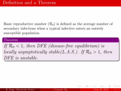
Basic reproductive number (R0) is defined as the average number ofsecondary infections when a typical infective enters an entirelysusceptible population.
Theorem
If R0 < 1, then DFE (disease-free equilibrium) islocally asymptotically stable(L.A.S.). If R0 > 1, thenDFE is unstable.
If you compute R0, you need not prove the stability of DFE.
B. Song (Montclair State) Compute R0 June 20, 2016 3 / 1
Definition and a Theorem
Basic reproductive number (R0) is defined as the average number ofsecondary infections when a typical infective enters an entirelysusceptible population.
Theorem
If R0 < 1, then DFE (disease-free equilibrium) islocally asymptotically stable(L.A.S.). If R0 > 1, thenDFE is unstable.
If you compute R0, you need not prove the stability of DFE.
B. Song (Montclair State) Compute R0 June 20, 2016 3 / 1

Two Types of Epidemiological Classes
• Let X be vector of infected classes, such asexposed, infectious, carrier, etc.
• Let Y be vector of uninfected classes, such assusceptible, recovered, etc.
B. Song (Montclair State) Compute R0 June 20, 2016 4 / 1

Two Types of Epidemiological Classes
• Let X be vector of infected classes, such asexposed, infectious, carrier, etc.
• Let Y be vector of uninfected classes, such assusceptible, recovered, etc.
B. Song (Montclair State) Compute R0 June 20, 2016 4 / 1
Rearrange System of Equations
dX
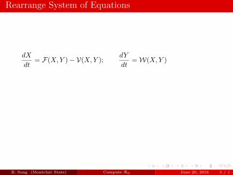
dt= F(X,Y )− V(X,Y );
dY
dt=W(X,Y )
F(X,Y ): Vector of new infection rates (flows from Y to X).V(X,Y ): Vector of all other rates (not new infection). These ratesinclude flows from X to Y (for instance, recovery rates), flows within Xand flows leaving from the system (for instance, death rates). For eachcompartment, in-flow in V is negative and out-flow in V is positive.DFE is (0, Y ).F(0, Y ) = 0 and V(0, Y ) = 0.
B. Song (Montclair State) Compute R0 June 20, 2016 5 / 1

Rearrange System of Equations
dX
dt= F(X,Y )− V(X,Y );
dY
dt=W(X,Y )
F(X,Y ): Vector of new infection rates (flows from Y to X).
V(X,Y ): Vector of all other rates (not new infection). These ratesinclude flows from X to Y (for instance, recovery rates), flows within Xand flows leaving from the system (for instance, death rates). For eachcompartment, in-flow in V is negative and out-flow in V is positive.DFE is (0, Y ).F(0, Y ) = 0 and V(0, Y ) = 0.
B. Song (Montclair State) Compute R0 June 20, 2016 5 / 1

Rearrange System of Equations
dX
dt= F(X,Y )− V(X,Y );
dY
dt=W(X,Y )
F(X,Y ): Vector of new infection rates (flows from Y to X).V(X,Y ): Vector of all other rates (not new infection). These ratesinclude flows from X to Y (for instance, recovery rates), flows within Xand flows leaving from the system (for instance, death rates). For eachcompartment, in-flow in V is negative and out-flow in V is positive.
DFE is (0, Y ).F(0, Y ) = 0 and V(0, Y ) = 0.
B. Song (Montclair State) Compute R0 June 20, 2016 5 / 1

Rearrange System of Equations
dX
dt= F(X,Y )− V(X,Y );
dY
dt=W(X,Y )
F(X,Y ): Vector of new infection rates (flows from Y to X).V(X,Y ): Vector of all other rates (not new infection). These ratesinclude flows from X to Y (for instance, recovery rates), flows within Xand flows leaving from the system (for instance, death rates). For eachcompartment, in-flow in V is negative and out-flow in V is positive.DFE is (0, Y ).
F(0, Y ) = 0 and V(0, Y ) = 0.
B. Song (Montclair State) Compute R0 June 20, 2016 5 / 1
Rearrange System of Equations
dX
dt= F(X,Y )− V(X,Y );
dY
dt=W(X,Y )
F(X,Y ): Vector of new infection rates (flows from Y to X).V(X,Y ): Vector of all other rates (not new infection). These ratesinclude flows from X to Y (for instance, recovery rates), flows within Xand flows leaving from the system (for instance, death rates). For eachcompartment, in-flow in V is negative and out-flow in V is positive.DFE is (0, Y ).F(0, Y ) = 0 and V(0, Y ) = 0.
B. Song (Montclair State) Compute R0 June 20, 2016 5 / 1

Jacobian around DFE
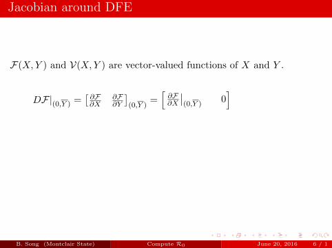
F(X,Y ) and V(X,Y ) are vector-valued functions of X and Y .
DF|(0,Y ) =[∂F∂X
∂F∂Y
](0,Y )
=[∂F∂X
∣∣(0,Y )
0]
DV|(0,Y ) =[∂V∂X
∂V∂Y
](0,Y )
=[∂V∂X
∣∣(0,Y )
0]
B. Song (Montclair State) Compute R0 June 20, 2016 6 / 1
Jacobian around DFE
F(X,Y ) and V(X,Y ) are vector-valued functions of X and Y .
DF|(0,Y ) =[∂F∂X
∂F∂Y
](0,Y )
=[∂F∂X
∣∣(0,Y )
0]
DV|(0,Y ) =[∂V∂X
∂V∂Y
](0,Y )
=[∂V∂X
∣∣(0,Y )
0]
B. Song (Montclair State) Compute R0 June 20, 2016 6 / 1

Jacobian around DFE
F(X,Y ) and V(X,Y ) are vector-valued functions of X and Y .
DF|(0,Y ) =[∂F∂X
∂F∂Y
](0,Y )
=[∂F∂X
∣∣(0,Y )
0]
DV|(0,Y ) =[∂V∂X
∂V∂Y
](0,Y )
=[∂V∂X
∣∣(0,Y )
0]
B. Song (Montclair State) Compute R0 June 20, 2016 6 / 1

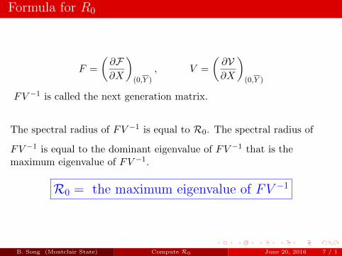
Formula for R0
F =
(∂F∂X
)(0,Y )
, V =
(∂V∂X
)(0,Y )
FV −1 is called the next generation matrix.
The spectral radius of FV −1 is equal to R0. The spectral radius of
FV −1 is equal to the dominant eigenvalue of FV −1 that is themaximum eigenvalue of FV −1.
R0 = the maximum eigenvalue of FV −1
B. Song (Montclair State) Compute R0 June 20, 2016 7 / 1

Formula for R0
F =
(∂F∂X
)(0,Y )
, V =
(∂V∂X
)(0,Y )
FV −1 is called the next generation matrix.
The spectral radius of FV −1 is equal to R0.
The spectral radius of
FV −1 is equal to the dominant eigenvalue of FV −1 that is themaximum eigenvalue of FV −1.
R0 = the maximum eigenvalue of FV −1
B. Song (Montclair State) Compute R0 June 20, 2016 7 / 1

Formula for R0
F =
(∂F∂X
)(0,Y )
, V =
(∂V∂X
)(0,Y )
FV −1 is called the next generation matrix.
The spectral radius of FV −1 is equal to R0. The spectral radius of
FV −1 is equal to the dominant eigenvalue of FV −1 that is themaximum eigenvalue of FV −1.
R0 = the maximum eigenvalue of FV −1
B. Song (Montclair State) Compute R0 June 20, 2016 7 / 1

Example 1: An SIR Model
Model Equations
dS
dt= Λ− βS I
N− µS,
dI
dt= βS
I
N− (µ+ γ)I,
dR
dt= γI − µR,
N = S + I +R.
DFE: (0,Λ/µ, 0)
F =
(∂F∂I
)∣∣∣∣(0,Λ/µ,0)
= β, V =
(∂V∂I
)∣∣∣∣(0,Λ/µ,0)
= µ+ γ
B. Song (Montclair State) Compute R0 June 20, 2016 8 / 1

Example 1: An SIR Model
Model Equations
dS
dt= Λ− βS I
N− µS,
dI
dt= βS
I
N− (µ+ γ)I,
dR
dt= γI − µR,
N = S + I +R.
Rearrange
X = I, Y = [S,R]T
F(I) = βSI
N,
V(I, S,R) = (µ+ γ)I
dI
dt= F(I)− V(I, S,R)
DFE: (0,Λ/µ, 0)
F =
(∂F∂I
)∣∣∣∣(0,Λ/µ,0)
= β, V =
(∂V∂I
)∣∣∣∣(0,Λ/µ,0)
= µ+ γ
B. Song (Montclair State) Compute R0 June 20, 2016 8 / 1

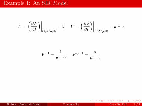
Example 1: An SIR Model
F =
(∂F∂I
)∣∣∣∣(0,Λ/µ,0)
= β, V =
(∂V∂I
)∣∣∣∣(0,Λ/µ,0)
= µ+ γ
V −1 =1
µ+ γ, FV −1 =
β
µ+ γ
R0 =β
µ+ γ
B. Song (Montclair State) Compute R0 June 20, 2016 9 / 1
Example 1: An SIR Model
F =
(∂F∂I
)∣∣∣∣(0,Λ/µ,0)
= β, V =
(∂V∂I
)∣∣∣∣(0,Λ/µ,0)
= µ+ γ
V −1 =1
µ+ γ, FV −1 =
β
µ+ γ
R0 =β
µ+ γ
B. Song (Montclair State) Compute R0 June 20, 2016 9 / 1

Example 1: An SIR Model
F =
(∂F∂I
)∣∣∣∣(0,Λ/µ,0)
= β, V =
(∂V∂I
)∣∣∣∣(0,Λ/µ,0)
= µ+ γ
V −1 =1
µ+ γ, FV −1 =
β
µ+ γ
R0 =β
µ+ γ
B. Song (Montclair State) Compute R0 June 20, 2016 9 / 1

Example 2: An SEIR Model
Model Equations
dS
dt= Λ− βS I
N− µS,
dE
dt= βS
I
N− (µ+ k + r1)E,
dI
dt= kE − (γ + µ)I,
dR
dt= r1E + γI − µR.
Rearrange Equations
X =
[EI
], Y =
[SR
]F =
[βS I
N0
]V =
[(µ+ k + r1)E−kE + (γ + µ)I
]
DFE: (0, 0,Λ/µ, 0)
B. Song (Montclair State) Compute R0 June 20, 2016 10 / 1

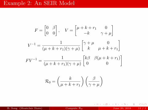
Example 2: An SEIR Model
F =
[0 β0 0
], V =
[µ+ k + r1 0−k γ + µ
]
V −1 =1
(µ+ k + r1)(γ + µ)
[γ + µ 0k µ+ k + r1
]
FV −1 =1
(µ+ k + r1)(γ + µ)
[kβ β(µ+ k + r1)0 0
]
R0 =
(k
µ+ k + r1
)(β
γ + µ
)
B. Song (Montclair State) Compute R0 June 20, 2016 11 / 1

Example 2: An SEIR Model
F =
[0 β0 0
], V =
[µ+ k + r1 0−k γ + µ
]
V −1 =1
(µ+ k + r1)(γ + µ)
[γ + µ 0k µ+ k + r1
]
FV −1 =1
(µ+ k + r1)(γ + µ)
[kβ β(µ+ k + r1)0 0
]
R0 =
(k
µ+ k + r1
)(β
γ + µ
)
B. Song (Montclair State) Compute R0 June 20, 2016 11 / 1

Example 2: An SEIR Model
F =
[0 β0 0
], V =
[µ+ k + r1 0−k γ + µ
]
V −1 =1
(µ+ k + r1)(γ + µ)
[γ + µ 0k µ+ k + r1
]
FV −1 =1
(µ+ k + r1)(γ + µ)
[kβ β(µ+ k + r1)0 0
]
R0 =
(k
µ+ k + r1
)(β
γ + µ
)
B. Song (Montclair State) Compute R0 June 20, 2016 11 / 1
Example 2: An SEIR Model
F =
[0 β0 0
], V =
[µ+ k + r1 0−k γ + µ
]
V −1 =1
(µ+ k + r1)(γ + µ)
[γ + µ 0k µ+ k + r1
]
FV −1 =1
(µ+ k + r1)(γ + µ)
[kβ β(µ+ k + r1)0 0
]
R0 =
(k
µ+ k + r1
)(β
γ + µ
)
B. Song (Montclair State) Compute R0 June 20, 2016 11 / 1
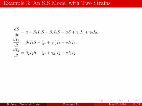
Example 3: An SIS Model with Two Strains
dS
dt= µ− β1I1S − β2I2S − µS + γ1I1 + γ2I2,
dI1
dt= β1I1S − (µ+ γ1)I1 + νI1I2,
dI2
dt= β2I2S − (µ+ γ2)I2 − νI1I2.
X =
[I1
I2
], Y = S, F =
[β1I1Sβ2I2S
], V =
[(µ+ γ1)I1 − νI1I2
(µ+ γ2)I2 + νI1I2
]DFE: (0, 0, 1)
B. Song (Montclair State) Compute R0 June 20, 2016 12 / 1
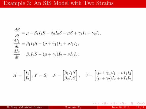
Example 3: An SIS Model with Two Strains
dS
dt= µ− β1I1S − β2I2S − µS + γ1I1 + γ2I2,
dI1
dt= β1I1S − (µ+ γ1)I1 + νI1I2,
dI2
dt= β2I2S − (µ+ γ2)I2 − νI1I2.
X =
[I1
I2
], Y = S, F =
[β1I1Sβ2I2S
], V =
[(µ+ γ1)I1 − νI1I2
(µ+ γ2)I2 + νI1I2
]
DFE: (0, 0, 1)
B. Song (Montclair State) Compute R0 June 20, 2016 12 / 1

Example 3: An SIS Model with Two Strains
dS
dt= µ− β1I1S − β2I2S − µS + γ1I1 + γ2I2,
dI1
dt= β1I1S − (µ+ γ1)I1 + νI1I2,
dI2
dt= β2I2S − (µ+ γ2)I2 − νI1I2.
X =
[I1
I2
], Y = S, F =
[β1I1Sβ2I2S
], V =
[(µ+ γ1)I1 − νI1I2
(µ+ γ2)I2 + νI1I2
]DFE: (0, 0, 1)
B. Song (Montclair State) Compute R0 June 20, 2016 12 / 1

Example 3: An SIS Model with Two Strains
F =
[f1
f2
]=
[β1I1Sβ2I2S
], V =
[v1
v2
]=
[(µ+ γ1)I1 − νI1I2
(µ+ γ2)I2 + νI1I2
]
F =
[∂f1∂I1
∂f1∂I2
∂f2∂I1
∂f2∂I2
](0,0,1)
=
[β1 00 β2
]
V =
[∂v1∂I1
∂v1∂I2
∂v2∂I1
∂v2∂I2
](0,0,1)
=
[µ+ γ1 0
0 µ+ γ2
], V −1 =
[1
µ+γ10
0 1µ+γ2
]
B. Song (Montclair State) Compute R0 June 20, 2016 13 / 1

Example 3: An SIS Model with Two Strains
F =
[β1 00 β2
], V −1 =
[1
µ+γ10
0 1µ+γ2
]
FV −1 =
[β1 00 β2
] [ 1µ+γ1
0
0 1µ+γ2
]=
[β1
µ+γ10
0 β2µ+γ2
]
R0 = max
{β1
µ+ γ1,
β2
µ+ γ2
}
B. Song (Montclair State) Compute R0 June 20, 2016 14 / 1

Example 3: An SIS Model with Two Strains
F =
[β1 00 β2
], V −1 =
[1
µ+γ10
0 1µ+γ2
]
FV −1 =
[β1 00 β2
] [ 1µ+γ1
0
0 1µ+γ2
]=
[β1
µ+γ10
0 β2µ+γ2
]
R0 = max
{β1
µ+ γ1,
β2
µ+ γ2
}
B. Song (Montclair State) Compute R0 June 20, 2016 14 / 1

Example 3: An SIS Model with Two Strains
F =
[β1 00 β2
], V −1 =
[1
µ+γ10
0 1µ+γ2
]
FV −1 =
[β1 00 β2
] [ 1µ+γ1
0
0 1µ+γ2
]=
[β1
µ+γ10
0 β2µ+γ2
]
R0 = max
{β1
µ+ γ1,
β2
µ+ γ2
}
B. Song (Montclair State) Compute R0 June 20, 2016 14 / 1
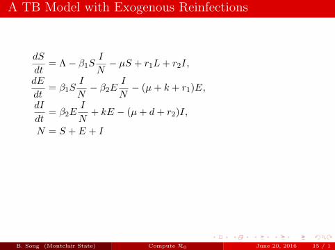
A TB Model with Exogenous Reinfections
dS
dt= Λ− β1S
I
N− µS + r1L+ r2I,
dE
dt= β1S
I
N− β2E
I
N− (µ+ k + r1)E,
dI
dt= β2E
I
N+ kE − (µ+ d+ r2)I,
N = S + E + I
X =
[EI
], Y = [S]
F =
[β1S
IN
0
], V =
[(µ+ k + r1)E + β2E
IN
−kE + (µ+ d+ r2)I − β2EIN
]
B. Song (Montclair State) Compute R0 June 20, 2016 15 / 1

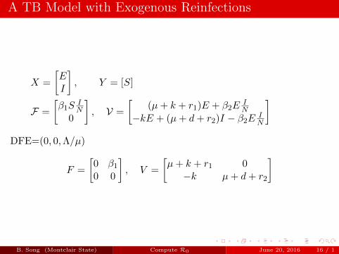
A TB Model with Exogenous Reinfections
X =
[EI
], Y = [S]
F =
[β1S
IN
0
], V =
[(µ+ k + r1)E + β2E
IN
−kE + (µ+ d+ r2)I − β2EIN
]DFE=(0, 0,Λ/µ)
F =
[0 β1
0 0
], V =
[µ+ k + r1 0−k µ+ d+ r2
]
B. Song (Montclair State) Compute R0 June 20, 2016 16 / 1
A TB Model with Exogenous Reinfections
X =
[EI
], Y = [S]
F =
[β1S
IN
0
], V =
[(µ+ k + r1)E + β2E
IN
−kE + (µ+ d+ r2)I − β2EIN
]DFE=(0, 0,Λ/µ)
F =
[0 β1
0 0
], V =
[µ+ k + r1 0−k µ+ d+ r2
]
B. Song (Montclair State) Compute R0 June 20, 2016 16 / 1

A TB Model with Exogenous Reinfections
F =
[0 β1
0 0
], V =
[µ+ k + r1 0−k µ+ d+ r2
]
V −1 =1
(µ+ k + r1)(µ+ d+ r2)
[µ+ d+ r2 0
k µ+ k + r1
]
FV −1 =1
(µ+ k + r1)(µ+ d+ r2)
[kβ1 β1(µ+ k + r1)0 0
]
R0 =
(β1
µ+ d+ r2
)(k
µ+ k + r1
)
B. Song (Montclair State) Compute R0 June 20, 2016 17 / 1

A TB Model with Exogenous Reinfections
F =
[0 β1
0 0
], V =
[µ+ k + r1 0−k µ+ d+ r2
]
V −1 =1
(µ+ k + r1)(µ+ d+ r2)
[µ+ d+ r2 0
k µ+ k + r1
]
FV −1 =1
(µ+ k + r1)(µ+ d+ r2)
[kβ1 β1(µ+ k + r1)0 0
]
R0 =
(β1
µ+ d+ r2
)(k
µ+ k + r1
)
B. Song (Montclair State) Compute R0 June 20, 2016 17 / 1

A TB Model with Exogenous Reinfections
F =
[0 β1
0 0
], V =
[µ+ k + r1 0−k µ+ d+ r2
]
V −1 =1
(µ+ k + r1)(µ+ d+ r2)
[µ+ d+ r2 0
k µ+ k + r1
]
FV −1 =1
(µ+ k + r1)(µ+ d+ r2)
[kβ1 β1(µ+ k + r1)0 0
]
R0 =
(β1
µ+ d+ r2
)(k
µ+ k + r1
)
B. Song (Montclair State) Compute R0 June 20, 2016 17 / 1

A TB Model with Exogenous Reinfections
F =
[0 β1
0 0
], V =
[µ+ k + r1 0−k µ+ d+ r2
]
V −1 =1
(µ+ k + r1)(µ+ d+ r2)
[µ+ d+ r2 0
k µ+ k + r1
]
FV −1 =1
(µ+ k + r1)(µ+ d+ r2)
[kβ1 β1(µ+ k + r1)0 0
]
R0 =
(β1
µ+ d+ r2
)(k
µ+ k + r1
)
B. Song (Montclair State) Compute R0 June 20, 2016 17 / 1


![LLVM MC in Practice · 2019. 10. 30. · _fac: push {r4, r7, lr} ldr! r0, [pc, #20] mov r1, #1 add r7, sp, #4 ldr! r0, [pc, r0] mov! r2, r1 ldr! r0, [r0] b! #0 # 4 bytes of data:.long](https://static.fdocuments.net/doc/165x107/60c63395503ad85a6a26c0e3/llvm-mc-in-practice-2019-10-30-fac-push-r4-r7-lr-ldr-r0-pc-20-mov.jpg)

