


Languages
Pages
Legal

Biological Stabilization of Municipal Solid Waste
Filipa Sofia Alves Ribeiro
Thesis to obtain the Master of Science Degree in
Biological Engineering
Supervisor(s): Prof. László Aleksza
Prof. Susete Maria Martins Dias
Examination Committee
Chairperson: Prof. Arsénio do Carmo Sales Mendes Fialho
Supervisor: Prof. Susete Maria Martins Dias
Member of the committee: Prof. Helena Maria Rodrigues Vasconcelos Pinheiro
November 2015

I
ACKNOWLEDGMENTS
It is a pleasure to thank to everyone who made this thesis possible by providing the support, help and
confidence needed.
Firstly, I would like to thank Professor László Aleksza for making possible this master's thesis at the
University Szent István Egytem in Hungary, and for the opportunity that I had to develop this work in an
international context.
A special thank you to Prof. Susete Dias for the transmission of knowledge, suggestions, availability,
friendliness and passion demonstrated in their research field.
To László Mathias, my lab partner for the company, sympathy and for all the information provided
about the work, including translations that were sometimes necessary.
To Sofia Tom and Aleomir Maciel, who I had the opportunity to meet during this stage, thank you for
the company, support, friendship and for having been part of this exceptional experience. They are special
people who I will never forget.
To colleagues and friends who were part of this route. A special thanks to Carla Morais, with whom I
did the last projects, for the bad and good moments spent and above all for the friendship and constant
support, to Marta Alves for friendship and all the unforgettable moments along this walk and to Chantel
Espadeiro for the unconditional support and because I know she is always there.
To my godmother, Isabel, for their support and confidence demonstrate since the first day.
To my sis to be part of my life, for always be present even when she was away, for the magic words
and unconditional love that she has always shown.
To Tokas, which was much more than a colleague who offered me, she is the friend of all moments,
the person who shows me every day the true meaning of friendship, she is who I take with me for life.
To my boyfriend for being a pillar in my life, for never let me fall and for the unconditional love he
shows me every day.
To my grandmother, who is somewhere proud and looking for me.
My deepest gratitude is to my parents, for making all this possible. Thank you for helping me to
overcome more this big step in my life. Thanks for the constant presence and support in difficult times.
Thank you for being who they are and for making me what I am today, with all the qualities and defects.

II
AGRADECIMENTOS
É com grande prazer que agradeço a todos aqueles que tornaram esta tese possível fornecendo o
suporte, ajuda e confiança necessários.
Em primeiro lugar gostaria de agradecer ao professor László Aleksza por ter tornado possível esta
dissertação de mestrado na Universidade Szent István Egytem na Hungria, e por ter tido a oportunidade de
desenvolver este trabalho num contexto internacional.
Um muito obrigada à professora Susete Dias por toda a transmissão de conhecimentos, sugestões,
disponibilidade, simpatia e paixão demonstrada na sua área de investigação.
Ao László Mathias, meu colega de laboratório, pela companhia, simpatia e por todos os esclarecimentos
fornecidos acerca do trabalho, incluindo as traduções algumas vezes necessárias.
À Sofia Ntoum e ao Maciel Aleomir, que tive oportunidade de conhecer durante esta etapa, obrigada pela
companhia, apoio, amizade e por terem feito parte desta experiência única, são pessoas especiais que nunca
esquecerei.
Aos colegas e amigos que fizeram parte deste percurso. Um obrigada especial à Carla Morais, com quem
fiz os últimos projetos, pelos maus e bons momentos passados e sobretudo pela amizade e apoio constantes, à
Marta Alves pela amizade e por todos os momentos inesquecíveis ao longo desta caminhada e à Chantel
Espadeiro pelo apoio incondicional e por saber que poderei sempre contar com ela.
À minha madrinha Isabel pelo apoio e confiança desde o primeiro dia.
À minha mana por fazer parte da minha vida, por estar sempre presente mesmo quando estava longe,
pelas palavras mágicas e amor incondicional que sempre demonstrou.
À Tokas, que foi muito mais do que uma colega que esta etapa me ofereceu, é a amiga de todos os
momentos, a pessoa que me demonstra todos os dias o verdadeiro sentido da amizade, é quem levo para a
vida.
Ao meu namorado, por ser um pilar na minha vida, por nunca me deixar cair e pelo amor incondicional
que demonstra todos os dias.
À minha avó que estará, em algum lugar, orgulhosa e a olhar por mim.
Aos meus pais, o mais profundo agradecimento, por terem tornado tudo isto possível. Obrigada por me
terem ajudado a ultrapassar mais esta grande etapa na minha vida. Obrigada pela presença constante e apoio

III
nos momentos mais difíceis. Obrigada por serem quem são e por terem feito de mim aquilo que sou hoje, com
todas as qualidades e defeitos.

IV
ABSTRACT
The biological stability of municipal solid waste is one of the main issues related to the evaluation of the
long-term emission potential and the environmental impact of landfills. The interest in mechanical biological
treatment (MBT) prior to landfilling is actually growing. It aims to reduce the mass and the volume of the waste.
Another target is a low environmental impact of the waste after its deposition.
The evaluation of biological activity of waste can be performed by respiration tests, such as the respiration
index at 4 days (AT4) determination. The aim of this study was to determinate the 4 days respiration index (AT4)
of municipal solid waste (MSW) after MBT with OxiTop® OC 110 controller B6M – 2.5, device.
The mechanical processing of municipal solid waste (MSW) took place in mechanical biological treatment
(MBT) plant of Zöld Híd Régió Environmental and Waste Ltd, located in Godollo, Hungary, where commingled
MSW was shredded using a hammer mill and was subsequently separated by size in a vibrating screen into
three different fractions – 35, 50 and 80 mm.
The composting process is conducted in adiabatic bioreactors of 80 liters, which ensure satisfactory
conditions for the control of the process, during four weeks – time of stabilization. Some parameters, such as
temperature and moisture, were measured over this time.
From available data in literature and according to European Union regulation, the processed MSW is fit for
landfilling if the respiration activity is below 10 mg O2/g dry mass over a period of 4 days. Respiration index of
three sizes of particles of waste was determined and followed during 4 weeks. In the end of the time of
stabilization the AT4 values obtained were 9, 18 and 23 mg O2/g DM for particle size of 35, 50 and 80 mm,
respectively.
KEYWORDS: municipal solid waste (MSW), mechanical biological treatment (MBT), composting, biological
stability, OxiTop, AT4.
V
RESUMO
A estabilidade biológica dos resíduos sólidos urbanos (RSU) é uma das principais questões relacionadas
com a avaliação do potencial de emissões a longo prazo e impacto ambiental dos aterros. O interesse no
tratamento mecânico e biológico antes da deposição em aterro está assim a crescer. O mesmo destina-se a
reduzir a massa e o volume dos resíduos. Outro alvo corresponde ao baixo impacto ambiental dos resíduos após
a sua deposição em aterro.
A avaliação da atividade biológica dos resíduos pode ser realizada por testes respirométricos, tais como a
determinação do índice de respiração ao fim de quatro dias (AT4). O objetivo deste estudo foi determinar o AT4
de resíduos sólidos urbanos, após tratamento mecânico e biológico, com o dispositivo de controlo OxiTop® OC
110 B6M – 2.5.
O tratamento mecânico dos resíduos sólidos urbanos decorreu na unidade de tratamento mecânico e
biológico Zöld Híd Régió Environmental and Waste Ltd, localizada na cidade de Godollo, Hungria, onde a mistura
de resíduos sólidos urbanos foi triturada com recurso a um moinho de martelos e posteriormente separada por
tamanhos em três frações distintas - 35, 50 e 80 mm, através duma peneira vibratória.
O processo de compostagem foi realizado em bio-reatores adiabáticos, onde foram garantidas condições
satisfatórias para o controlo do processo, durante quatro semanas – tempo de estabilização. Ao longo deste
período foram monitorizados alguns parâmetros, tais como temperatura e humidade.
A partir de dados disponíveis na literatura e de acordo com a União Europeia, os resíduos sólidos
urbanos estão aptos para a deposição em aterro se a atividade respiratória for inferior a 10 mgO2/ g de massa
seca ao fim dum período de quatro dias. O índice de respiração das três frações de RSU foi determinado e
seguido ao longo do tempo de estabilização, sendo que no final deste tempo os valores de AT4 obtidos foram de
9, 18 e 23 mgO2/ g de massa seca para os tamanhos de partículas de 35, 50 e 80 mm, respetivamente.
PALAVRAS-CHAVE: resíduos sólidos urbanos (RSU), tratamento mecânico e biológico, compostagem, estabilidade
biológica, OxiTop, AT4.
VI
TABLE OF CONTENTS
1 Introduction ........................................................................................................................................ 1
1.1 Background ................................................................................................................................... 1
1.2 Water And Waste Management Research Group ......................................................................... 2
1.3 Research goals ............................................................................................................................. 2
2 Literature review ................................................................................................................................ 3
2.1 Municipal solid waste management .............................................................................................. 3
2.1.1 Municipal solid waste Management: Legal framework in Portugal ....................................... 4
2.1.2 Waste Management: Legal framework in Hungary ............................................................... 7
2.2 Mechanical biological treatment .................................................................................................... 9
2.2.1 Mechanical treatment ......................................................................................................... 10
2.2.2 Biological treatment ............................................................................................................ 11
2.3 Composting process .................................................................................................................... 12
2.3.1 Process description ............................................................................................................ 13
2.3.2 Composting systems .......................................................................................................... 13
2.3.2.1 Windrow ......................................................................................................................... 14
2.3.2.2 Static pile ....................................................................................................................... 14
2.3.2.3 In-vessel ........................................................................................................................ 14
2.3.3 Composting stages ............................................................................................................. 15
2.3.4 Conditions and components affecting composting process ................................................ 16
2.3.4.1 Nature of the substrate .................................................................................................. 16
2.3.4.2 Aeration and Oxygen ..................................................................................................... 17
2.3.4.3 Moisture ......................................................................................................................... 17
2.3.4.4 Particle size ................................................................................................................... 17
2.3.4.5 Porosity and Free air space ........................................................................................... 17
2.3.4.6 Size of compost system ................................................................................................. 18
2.3.4.7 Mixing/Turning ............................................................................................................... 18
2.3.4.8 Temperature .................................................................................................................. 18
2.3.4.9 Nutrients ........................................................................................................................ 19

VII
2.3.4.10 Carbon-to-nitrogen ratio ............................................................................................... 19
2.3.4.11 pH ................................................................................................................................ 19
2.3.4.12 Odor ............................................................................................................................. 20
2.3.4.13 Microorganisms ........................................................................................................... 20
2.4 Biological stability ........................................................................................................................ 21
2.4.1 Respirometric methods ....................................................................................................... 22
2.4.1.1 Self-heating test ............................................................................................................. 23
2.4.1.2 Methods based on CO2 production ................................................................................ 23
2.4.1.3 Methods based on O2 uptake ........................................................................................ 23
3 Materials and Methods .................................................................................................................... 26
3.1 Mechanical-biological treatment plant ......................................................................................... 26
3.2 Materials ...................................................................................................................................... 27
3.3 Samples ...................................................................................................................................... 29
3.4 Bulk density determination .......................................................................................................... 29
3.5 Moisture determination ................................................................................................................ 29
3.5.1 Experimental apparatus ...................................................................................................... 30
3.5.2 OUR and SOUR ................................................................................................................. 32
3.5.3 AT4 ...................................................................................................................................... 33
4 Results and discussion .................................................................................................................... 34
4.1 Moisture ...................................................................................................................................... 34
4.2 Temperature ................................................................................................................................ 35
4.3 Bulk Density ................................................................................................................................ 37
4.4 Tests on OxiTop .......................................................................................................................... 38
4.4.1 Measurement adaptations .................................................................................................. 38
4.4.2 OUR and SOUR ................................................................................................................. 39
4.4.3 AT4 ...................................................................................................................................... 48
5 Conclusions ..................................................................................................................................... 51
6 References ...................................................................................................................................... 53
Appendices ................................................................................................................................................ 56

VIII
Appendix A ................................................................................................................................................. 57
Appendix B ................................................................................................................................................. 58
IX
LIST OF TABLES
Table 2-1 Different options for waste classification/separation used in MBT plants. ................................. 10
Table 2-2 Comparison of aerobic and anaerobic processes for processing the OFMSW. ........................ 11
Table 2-3 Advantages and disadvantages of the composting process. ..................................................... 12
Table 2-4 Temperature and the Time Interval Required to Destroy Most Common Types of Pathogenic
Microorganisms and Parasites. ............................................................................................................................. 19
Table 2-5 List of major microorganisms present in compost. ..................................................................... 21
Table 2-6 Most commonly used respiration indices bases on O2 uptake. .................................................. 25
Table 4-1 Moisture content in dry basis for each MSW fraction at the end of each week of biological
stabilization, at room temperature. The results are average (N=3). ...................................................................... 34
Table 4-2 Bulk density in wet basis for the three different MSW fractions at the end of each week of
biological stabilization. ........................................................................................................................................... 37
Table 4-3 Values of oxygen uptake rate (OUR) measured on OxiTop over 7 days and respective total
solids (TS) contained on each OxiTop vessel, for MSW samples of 35 mm. ........................................................ 45
Table 4-4 Values of oxygen uptake rate (OUR) measured on OxiTop over 7 days and respective total
solids (TS) contained on each OxiTop vessel, for MSW samples of 50 mm. ........................................................ 45
Table 4-5 Values of oxygen uptake rate (OUR) measured on OxiTop over 7 days and respective total
solids (TS) contained on each OxiTop vessel, for MSW samples of 50 mm. ........................................................ 46
Table 4-6 Time of lag phase (days) observed for different MSW samples during measurement of oxygen
consumption. ......................................................................................................................................................... 46
Table 4-7 Time of lag phase and Specific oxygen uptake rate (SOUR) for the three fractions of MSW at
the end of each week of composting process, measured in Oxitop during seven days. The results are average ±
stdev (N=3). ........................................................................................................................................................... 47
X
LIST OF FIGURES
Figure 2-1 Hierarchy of waste according to European Union. ..................................................................... 3
Figure 2-2 Municipal waste generated per capita in 36 European Countries in 2004 and 2012, (SOER,
2015). ...................................................................................................................................................................... 4
Figure 2-3 Waste generated in Portugal, Source: Eurostat. ........................................................................ 5
Figure 2-4 Destination of Portuguese MSW generated in 2012, (Dias, et al., 2015). .................................. 6
Figure 2-5 Representative physical composition of Portuguese MSW (Agência Portuguesa do Ambiente,
2014). ...................................................................................................................................................................... 6
Figure 2-6 Waste treatment methods used in Hungary, 2009 (Dienes, 2012). ............................................ 7
Figure 2-7 Waste generated in Hungary, Source: Eurostat ......................................................................... 8
Figure 2-8 Representative physical composition of Hungarian MSW (Orosz & Fazekas, 2008). ................ 8
Figure 2-9 Simplified flow diagram of an aerobic MBT plant type, adapted from (Dias, et al., 2014). ......... 9
Figure 2-10 Generalized flow diagram for the composting process, adapted from (Tchobanoglous, et al.,
1993). .................................................................................................................................................................... 13
Figure 2-11 Typical temperature and pH variation during composting process-The three stages of
composting, adapted from (Trautmann & Krasny, 1997). ...................................................................................... 15
Figure 3-1 Simplified scheme of MSW treatment in MBT plant Zöld Híd Régió Environmental and Waste
Ltd, before the MSW are sent to the laboratory for biological treatment: 1) Hammer mill and 2) Vibrating screen.
.............................................................................................................................................................................. 26
Figure 3-2 Mechanical Biological Treatment plant Zöld Híd Régió Environmental and Waste Ltd: 1)
composting area and 2) MSW reception and pre-treatment. ................................................................................. 27
Figure 3-3 Scheme of composting adiabatic bioreactor. ........................................................................... 28
Figure 3-4 Simplified scheme of all three adiabatic reactors. .................................................................... 29
Figure 3-5 Scheme of the vessel with measuring head ............................................................................. 31
Figure 3-6 a) OxiTop vessels containing samples, absorbent and negative pressure sensors and b)
thermostat cabinet with OxiTop vessels. ............................................................................................................... 31
Figure 3-7 OxiTop Control System. ........................................................................................................... 32
Figure 4-1 Relationship between the temperature, measured during the composting process in the bio-
reactors with a 30dm3.min-1 air flow provided for 2 minutes every 20 minutes , and moisture measured at the end
of each week of biological stabilization at room temperature. a) MSW fraction of 35 mm; b) MSW fraction of 50
mm and c) MSW fraction of 80 mm. ...................................................................................................................... 36
Figure 4-2 Recorded oxygen consumption of 35 mm fraction of MSW by sensors in 0 week (before
treatment), in three replicates, before of correction. .............................................................................................. 38
Figure 4-3 Total amount of consumed oxygen of 35 mm fraction of MSW in 0 week (before treatment), in
three replicates, after correction. ........................................................................................................................... 39
XI
Figure 4-4 OxiTop oxygen consumption over the week , of MSW as received, at 20ºC1: a) three
repetitions of the grab sample of 35 mm; b) three repetitions of the grab sample of 50 mm; c) two repetitions of
the grab sample of 80 mm. .................................................................................................................................... 40
Figure 4-5 OxiTop oxygen consumption over the week, after the first week of biological stabilization of
MSW, at 20ºC1: a) three repetitions of the grab sample of 35 mm; b) two repetitions of the grab sample of 50
mm; c) two repetitions of the grab sample of 80 mm. ............................................................................................ 41
Figure 4-6 OxiTop oxygen consumption over the week, after the second week of biological stabilization of
MSW, at 20ºC1: a) two repetitions of the grab sample of 35 mm; b) three repetitions of the grab sample of 50
mm; c) two repetitions of the grab sample of 80 mm. ............................................................................................ 42
Figure 4-7 OxiTop oxygen consumption over the week, after the third week of biological stabilization of
MSW, at 20ºC1: a) the grab sample of 35 mm; b) two repetitions of the grab sample of 50 mm; c) two repetitions
of the grab sample of 80 mm. ................................................................................................................................ 43
Figure 4-8 OxiTop oxygen consumption over the week, after the fourth week of biological stabilization of
MSW, at 20ºC1: a) two repetitions of the grab sample of 35 mm; b) three repetitions of the grab sample of 50
mm; c) two repetitions of the grab sample of 80 mm. ............................................................................................ 44
Figure 4-9 AT4 values between 0 and 4 weeks for MSW fraction of 35 mm. ............................................. 48
Figure 4-10 AT4 values between 0 and 4 weeks for MSW fraction of 50 mm. ........................................... 48
Figure 4-11 AT4 values between 0 and 4 weeks for MSW fraction of 80 mm. ........................................... 49
XII
LIST OF ABBREVIATIONS
A
AD – Anaerobic digestion
AT4 – Respiration index at 4 days
AT7 – Respiration index at 7 days
B
BD – Bulk density
BMW – Biodegradable municipal waste
D
DM – Dry mass
DRI – Dynamic respiration index
DRT – Dynamic respiration test
DSOUR – Dry specific oxygen uptake rate
E
EEA – European economic area
EU – European Union
F
FAS – Free air space
Fe – Ferrous
G
GHG – Greenhouse gas
M
MBT – Mechanical-biological treatment
MC – Moisture content
MSW – Municipal Solid Waste
N
NWMP – National Waste Management Plans

XIII
O
OD – Oxygen demand
OFMSW – Organic fraction of municipal solid waste
OUR – Oxygen uptake rate
P
PDRI – Potential dynamic respiration index
PERSU I – Plano estratégico para os resíduos sólidos urbanos I/ First national strategic plan for MSW
PERSU II – Plano estratégico para os resíduos sólidos urbanos II/ Second national strategic plan for MSW
R
RDRI – Real dynamic respiration index
RDF – Refuse derived fuels
S
SOUR – Specific oxygen uptake rate
SRI – Static respiration index
SRT – Static respiration test
T
T – Temperature
TS – Total solids
1
1 INTRODUCTION
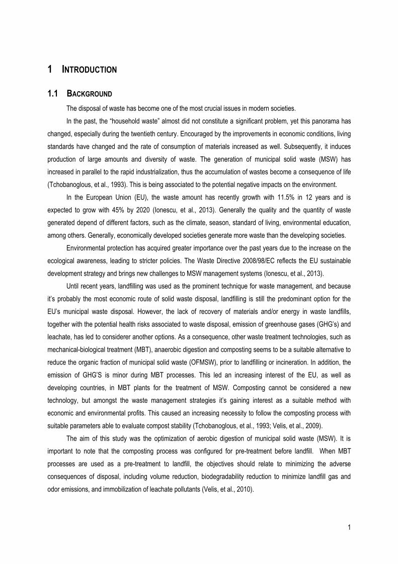
1.1 BACKGROUND
The disposal of waste has become one of the most crucial issues in modern societies.
In the past, the “household waste” almost did not constitute a significant problem, yet this panorama has
changed, especially during the twentieth century. Encouraged by the improvements in economic conditions, living
standards have changed and the rate of consumption of materials increased as well. Subsequently, it induces
production of large amounts and diversity of waste. The generation of municipal solid waste (MSW) has
increased in parallel to the rapid industrialization, thus the accumulation of wastes become a consequence of life
(Tchobanoglous, et al., 1993). This is being associated to the potential negative impacts on the environment.
In the European Union (EU), the waste amount has recently growth with 11.5% in 12 years and is
expected to grow with 45% by 2020 (Ionescu, et al., 2013). Generally the quality and the quantity of waste
generated depend of different factors, such as the climate, season, standard of living, environmental education,
among others. Generally, economically developed societies generate more waste than the developing societies.
Environmental protection has acquired greater importance over the past years due to the increase on the
ecological awareness, leading to stricter policies. The Waste Directive 2008/98/EC reflects the EU sustainable
development strategy and brings new challenges to MSW management systems (Ionescu, et al., 2013).
Until recent years, landfilling was used as the prominent technique for waste management, and because
it’s probably the most economic route of solid waste disposal, landfilling is still the predominant option for the
EU’s municipal waste disposal. However, the lack of recovery of materials and/or energy in waste landfills,
together with the potential health risks associated to waste disposal, emission of greenhouse gases (GHG’s) and
leachate, has led to considerer another options. As a consequence, other waste treatment technologies, such as
mechanical-biological treatment (MBT), anaerobic digestion and composting seems to be a suitable alternative to
reduce the organic fraction of municipal solid waste (OFMSW), prior to landfilling or incineration. In addition, the
emission of GHG’S is minor during MBT processes. This led an increasing interest of the EU, as well as
developing countries, in MBT plants for the treatment of MSW. Composting cannot be considered a new
technology, but amongst the waste management strategies it’s gaining interest as a suitable method with
economic and environmental profits. This caused an increasing necessity to follow the composting process with
suitable parameters able to evaluate compost stability (Tchobanoglous, et al., 1993; Velis, et al., 2009).
The aim of this study was the optimization of aerobic digestion of municipal solid waste (MSW). It is
important to note that the composting process was configured for pre-treatment before landfill. When MBT
processes are used as a pre-treatment to landfill, the objectives should relate to minimizing the adverse
consequences of disposal, including volume reduction, biodegradability reduction to minimize landfill gas and
odor emissions, and immobilization of leachate pollutants (Velis, et al., 2010).
2
1.2 WATER AND WASTE MANAGEMENT RESEARCH GROUP
This study was supported by the department of Water and Waste Management of the Szent István
University, Faculty of Agricultural and Environmental Sciences, in Gödöllő, Hungary, for a period of six months.
The group develops work in different research areas, such as, Waste Management, Biological Waste Treatment,
Composting, Production of Biogas, Wastewater treatment, Water Management, among others. The group also
has some business partnerships in countries like Germany and Austria.
1.3 RESEARCH GOALS
The main goal of this study was the characterization of the biological stability of the municipal solid waste
during the biological process by means of respiration activity.
To study of bio-stabilization process using adiabatic reactors:
o Monitoring the effectiveness of the biodegradation process in the production of compost
material from collected organic fractions of municipal solid waste;
o Assessment of the reduction in the biological activity of solid waste stabilized in aerobic
conditions.
To investigate the different parameters of MSW during biological process:
o Moisture content;
o Temperature;
o Bulk Density.
To determine the 4 days respiration index (AT4) of MSW during the time of stabilization:
o Assessment of the biological activity or the degree of maturity of the stabilized materials in the
aerobic conditions.
3
2 LITERATURE REVIEW
2.1 MUNICIPAL SOLID WASTE MANAGEMENT
Increasing population levels, booming economy, rapid urbanization and the rise in community living
standards have greatly accelerated the municipal solid waste generation rate in developing countries. The
production of large amounts and diversity of waste is being associated to the potential negative impacts on the
environment. Subsequently, it was necessary to create legislation to control the production of waste and resource
depletion. European Union was producing legislation addressing the issue of waste and its deposition, by
directives, enriched the national legislation of its Member States.
Management of MSW represents an important role in sustainable development. The definition of municipal
waste used in different countries varies, reflecting diverse waste management practices. According to European
Landfill Directive, 1999/31/EC, municipal waste is defined as, “waste from households, as well as other waste
which, because of its nature or composition, is similar to waste from household.” This includes appliances,
furniture, residential garden waste and domestic hazardous waste. In the same Directive, biodegradable
municipal waste (BMW) is defined as “any waste that is capable of undergoing anaerobic or aerobic
decomposition as food, garden waste and paper”, which includes food wastes, garden wastes, paper/cardboard,
textiles and wood. The Landfill Directive 99/31/EC obliges the EU Member States to reduce the amount of
biodegradable waste that they landfill to 35% of the amount of BMW that was landfilled in 1995. Municipal waste
management in European countries has evolved over the last two decades from a focus on disposal methods to a
greater focus on prevention and recycling. Currently EU waste policy is based on a concept known as “The waste
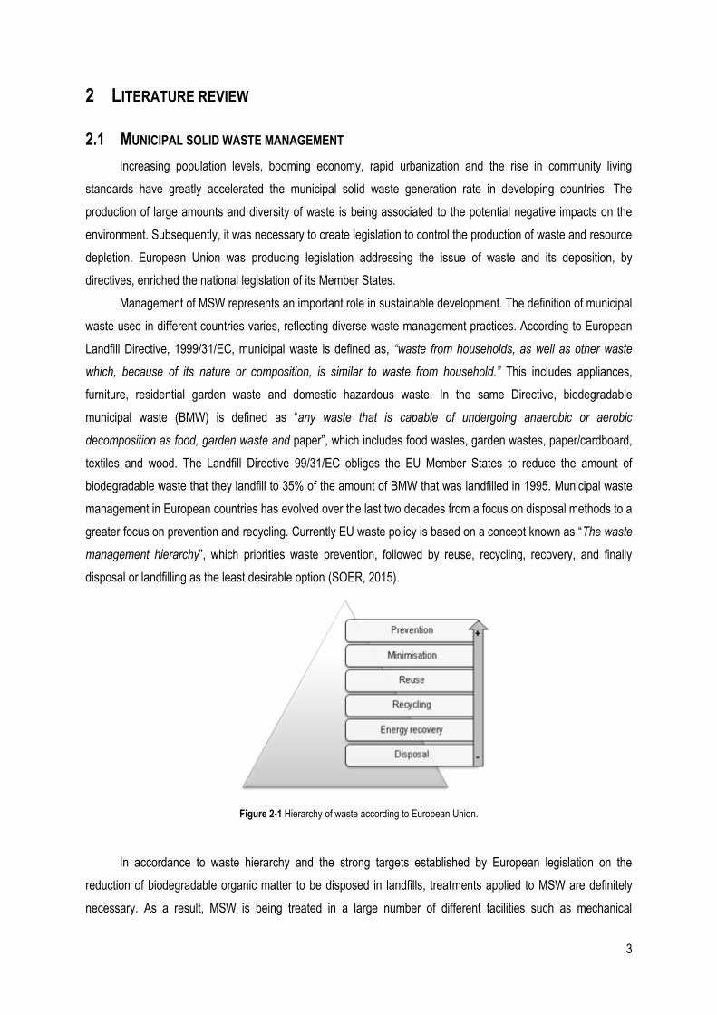
management hierarchy”, which priorities waste prevention, followed by reuse, recycling, recovery, and finally
disposal or landfilling as the least desirable option (SOER, 2015).
Figure 2-1 Hierarchy of waste according to European Union.
In accordance to waste hierarchy and the strong targets established by European legislation on the
reduction of biodegradable organic matter to be disposed in landfills, treatments applied to MSW are definitely
necessary. As a result, MSW is being treated in a large number of different facilities such as mechanical
4
biological treatment (MBT), anaerobic digestion and composting plants. The main objective of these plants is to
reduce the content of waste biodegradable organic matter and consequently to reduce its environmental impacts,
such as GHG and odor emissions, and soil and groundwater contamination (Barrena, et al., 2009).
Waste represents an enormous loss of resources in the form of both materials and energy. The amount of
waste generated can be seen as an indicator of how efficient we are as a society, particularly in relation to our
use of natural resources and waste treatment operations. Municipal waste constitutes only around 10% of total
waste generated, but because of its complex character and its distribution among many waste generators,
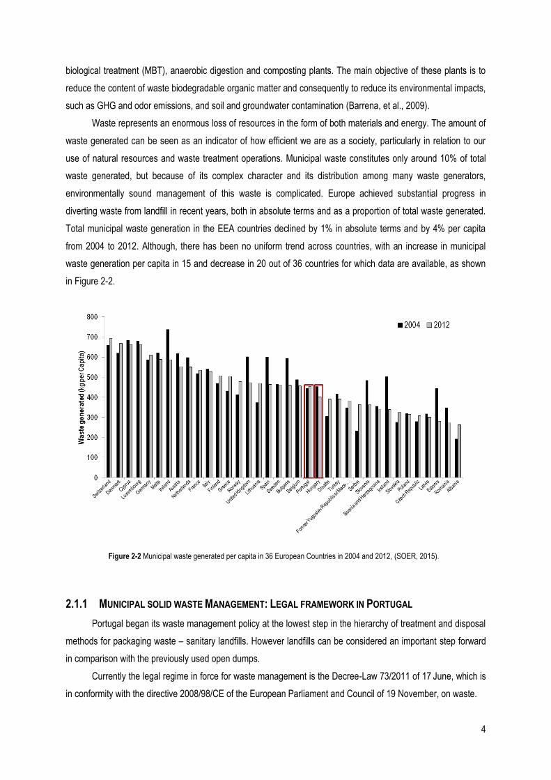
environmentally sound management of this waste is complicated. Europe achieved substantial progress in
diverting waste from landfill in recent years, both in absolute terms and as a proportion of total waste generated.
Total municipal waste generation in the EEA countries declined by 1% in absolute terms and by 4% per capita
from 2004 to 2012. Although, there has been no uniform trend across countries, with an increase in municipal
waste generation per capita in 15 and decrease in 20 out of 36 countries for which data are available, as shown
in Figure 2-2.
2.1.1 MUNICIPAL SOLID WASTE MANAGEMENT: LEGAL FRAMEWORK IN PORTUGAL
Portugal began its waste management policy at the lowest step in the hierarchy of treatment and disposal
methods for packaging waste – sanitary landfills. However landfills can be considered an important step forward
in comparison with the previously used open dumps.
Currently the legal regime in force for waste management is the Decree-Law 73/2011 of 17 June, which is
in conformity with the directive 2008/98/CE of the European Parliament and Council of 19 November, on waste.
Figure 2-2 Municipal waste generated per capita in 36 European Countries in 2004 and 2012, (SOER, 2015).

5
The first strategic plan of solid wastes, known as PERSU I (National strategic plan for MSW), arose in
1997 by the European Directive 75/442/EEC. The main objective of the PERSU I was to eliminate open dumps
and divert the waste, according to specific quantified targets, to recycling, incineration and composting (Magrinho,
et al., 2006). The PERSU I covered the period until 2006. In 2007, PERSU II substituted PERSU I and it will be
operational until 2016. Its principal goals are to eliminate inefficiencies observed in the implementation of the
PERSU I, such as, adapt EU legislation to Portuguese reality; rationalize the costs; encourage participation of all
stakeholders, based on input from all of them; support incineration with energy recovery and MBT as solutions to
MSW treatment; introduce separate collection of organic wastes and other measures to divert them from landfills,
and maximize by-products utilization (Bakas, 2013).
2002 was the first year that reliable data on MSW generation could be obtained, and nowadays there is
official data thanks to strategic plans PERSU I and PERSU II (Teixeira, et al., 2014).
The total production of MSW in Portugal continental was, in 2012, approximately 4.5 million tons, which
correspond to an annual per capita of 454 kg/hab.year, i.e. a daily production of municipal waste of 1.24 kg per
inhabitant. This represents a decrease of about 7.4% compared to 2011. In 2012, in Portugal continental, the total
municipal waste collected, 85.9% comes from collection undifferentiated and 1401% of separate collection. In
regional terms it appears that in 2012, at the continental level, the region of Lisbon and Vale do Tejo had the
highest production of municipal waste, followed by the North region, with 37.6 and 32.5%, respectively (Agência
Portuguesa do Ambiente, 2014).
Figure 2-3 Waste generated in Portugal, Source: Eurostat.
Landfilling, the last choice method in the waste management hierarchy, is the method that has been
adopted by the majority of management entities for MSW treatment in Portugal, which may be explained by three
main factors: the small capacity of management entities of MSW, the low installation and operating costs of
landfills, and the existence of considerable available space to locate the landfills (Magrinho, et al., 2006).
4,665 4,745
4,898 4,967
5,472 5,496 5,457
5,178
4,766
4,598
4
4,2
4,4
4,6
4,8
5
5,2
5,4
5,6
2004 2005 2006 2007 2008 2009 2010 2011 2012 2013
Was
te g
ener
ated
(mill
ion
tons
)
Years
6
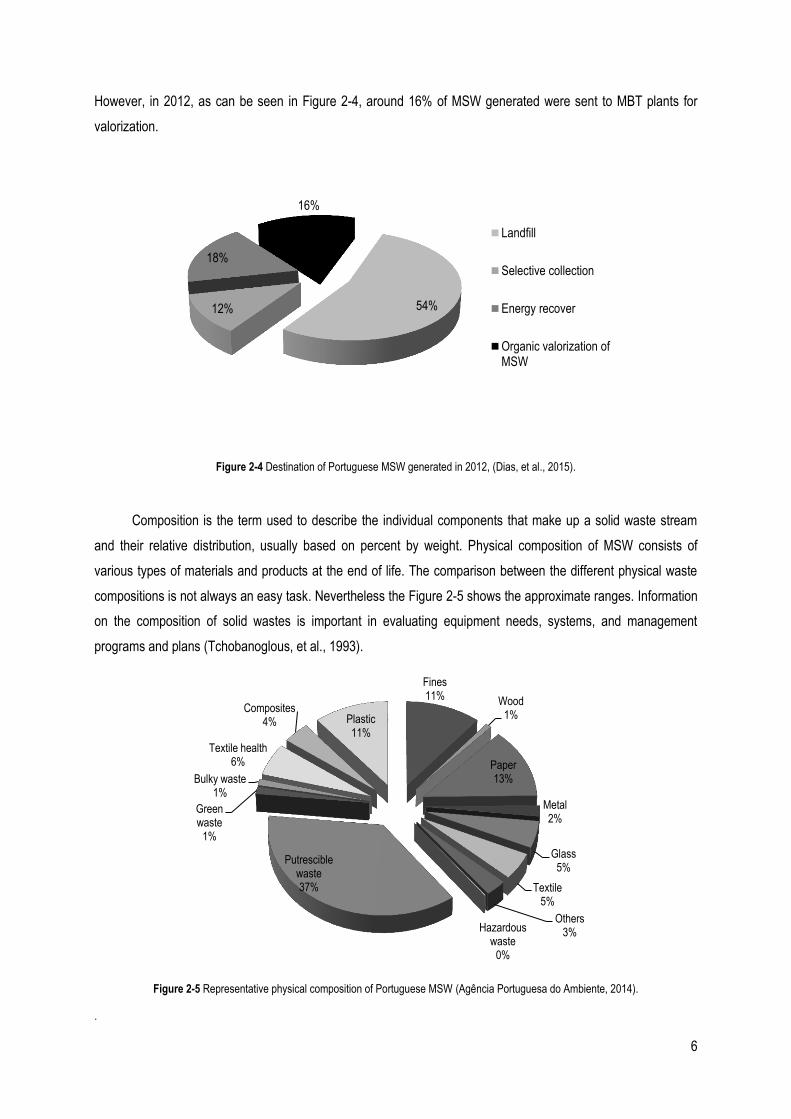
However, in 2012, as can be seen in Figure 2-4, around 16% of MSW generated were sent to MBT plants for
valorization.
Figure 2-4 Destination of Portuguese MSW generated in 2012, (Dias, et al., 2015).
Composition is the term used to describe the individual components that make up a solid waste stream
and their relative distribution, usually based on percent by weight. Physical composition of MSW consists of
various types of materials and products at the end of life. The comparison between the different physical waste
compositions is not always an easy task. Nevertheless the Figure 2-5 shows the approximate ranges. Information
on the composition of solid wastes is important in evaluating equipment needs, systems, and management
programs and plans (Tchobanoglous, et al., 1993).
Figure 2-5 Representative physical composition of Portuguese MSW (Agência Portuguesa do Ambiente, 2014).
.
54% 12%
18%
16%
Landfill
Selective collection
Energy recover
Organic valorization ofMSW
Fines 11% Wood
1%
Paper 13%
Metal 2%
Glass 5%
Textile 5%
Others 3% Hazardous
waste 0%
Putrescible waste 37%
Green waste
1%
Bulky waste 1%
Textile health 6%
Composites 4% Plastic
11%
7
2.1.2 WASTE MANAGEMENT: LEGAL FRAMEWORK IN HUNGARY
The Hungarian waste management regime is being developed continuously, especially from the beginning
of the EU accession procedure in the late 90’s. The framework legislation has been established by the Act
number 53 of 2000 on Waste Management in conformity with the EU directive 2006/12/EC, on waste. Aims, tasks
and priorities of medium term development plans of national waste management were defined in the National
Waste Management Plans (NWMP) prepared for six-year periods. The first NWMP was valid for the period of
2003-2008, and the second for the next planning period, 2009-2014 (Orosz & Fazekas, 2008; Herczeg, 2013).
For decades, the dominant treatment of municipal waste in Hungary was landfilling. In the past, almost all
municipalities operated one or more landfill sites, generally not constructed and equipped with technologies of
modern waste management. These sites were basically waste dumps operated by the local councils at that time
(Herczeg, 2013).
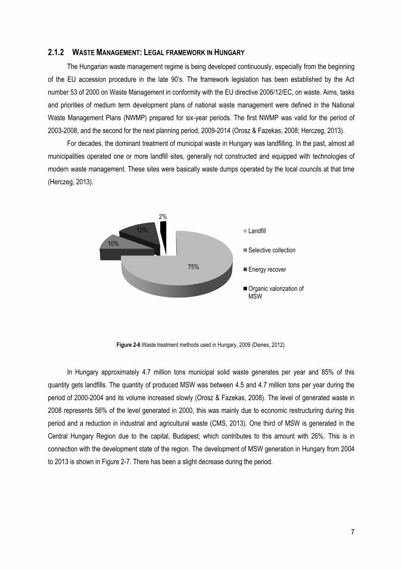
Figure 2-6 Waste treatment methods used in Hungary, 2009 (Dienes, 2012).
In Hungary approximately 4.7 million tons municipal solid waste generates per year and 85% of this
quantity gets landfills. The quantity of produced MSW was between 4.5 and 4.7 million tons per year during the
period of 2000-2004 and its volume increased slowly (Orosz & Fazekas, 2008). The level of generated waste in
2008 represents 56% of the level generated in 2000, this was mainly due to economic restructuring during this
period and a reduction in industrial and agricultural waste (CMS, 2013). One third of MSW is generated in the
Central Hungary Region due to the capital, Budapest, which contributes to this amount with 26%. This is in
connection with the development state of the region. The development of MSW generation in Hungary from 2004
to 2013 is shown in Figure 2-7. There has been a slight decrease during the period.
75%
10%
13%
2%
Landfill
Selective collection
Energy recover
Organic valorization ofMSW

8
Figure 2-7 Waste generated in Hungary, Source: Eurostat
Hungary has made a rapid progress towards diversion of BMW from landfill. Intermediate targets set for
2006 and 2009 by the Landfill Directive, were met with achieving a reduction to 66% in 2006 and 46% in 2009,
mainly due to a dramatic increase in material recovery, MBT and due to an improved separate paper collection
system.
Regarding the physical composition of municipal waste, it has not changed in the last decade. One third of
the waste consists of metal glass, plastic and paper packaging and the other third is biodegradable organic
materials (Orosz & Fazekas, 2008).
Figure 2-8 Representative physical composition of Hungarian MSW (Orosz & Fazekas, 2008).
4,592 4,646
4,711
4,594 4,553
4,312
4,033
3,809
3,988
3,738
3,5
3,7
3,9
4,1
4,3
4,5
4,7
4,9
2004 2005 2006 2007 2008 2009 2010 2011 2012 2013
Was
te g
ener
ated
(mill
ion
tons
)
Years
Organic matter 38%
Paper 14%
Plastic 12%
Metal 4%
Others 25%
Textile 3%
Glass 4%
9
2.2 MECHANICAL BIOLOGICAL TREATMENT
Mechanical biological treatment of waste is the processing or conversation waste from human settlements
with biologically degradable components via combination of mechanical and other physical processes with
biological processes. It is applicable for the treatment of waste prior to depositing, but also for the production of
refused derived fuels (RDF). Waste treatment plants defined as MBT integrate mechanical processing, such as
size reduction and air classification, with bio-conversation reactors, such as composting or anaerobic digestion.
MBT plants can incorporate a number of different processes in a variety of combinations. Over the last 15 years
MBT technologies have established their presence in Europe. MBT is emerging as an attractive option for
developing countries as well (Soyes & Plickert, 2002; Velis, et al., 2009).
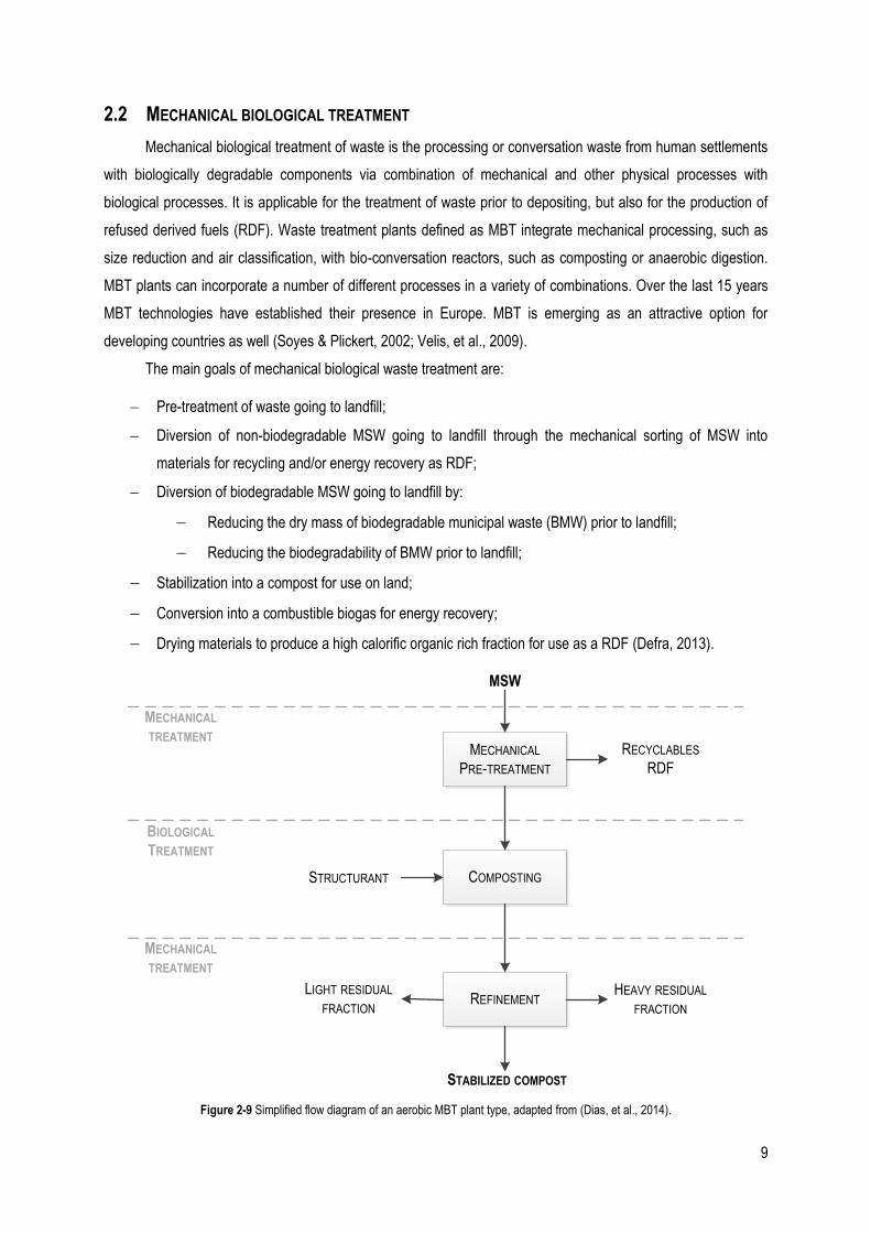
The main goals of mechanical biological waste treatment are:
Pre-treatment of waste going to landfill;
Diversion of non-biodegradable MSW going to landfill through the mechanical sorting of MSW into
materials for recycling and/or energy recovery as RDF;
Diversion of biodegradable MSW going to landfill by:
Reducing the dry mass of biodegradable municipal waste (BMW) prior to landfill;
Reducing the biodegradability of BMW prior to landfill;
Stabilization into a compost for use on land;
Conversion into a combustible biogas for energy recovery;
Drying materials to produce a high calorific organic rich fraction for use as a RDF (Defra, 2013).
MECHANICAL
PRE-TREATMENT
COMPOSTING
REFINEMENT
MSW
RECYCLABLES
RDF
STRUCTURANT
LIGHT RESIDUAL
FRACTION
HEAVY RESIDUAL
FRACTION
STABILIZED COMPOST
MECHANICAL
TREATMENT
MECHANICAL
TREATMENT
BIOLOGICAL
TREATMENT
Figure 2-9 Simplified flow diagram of an aerobic MBT plant type, adapted from (Dias, et al., 2014).
10
In general, quantity and quality of the outputs of an MBT plant vary in function of:
The characteristics of the inputs, which depend on the area and season of production;
The type and percentage of materials that are source separated;
The types of mechanical and biological processing units employed in the plant (Di Lonardo, et al., 2012).
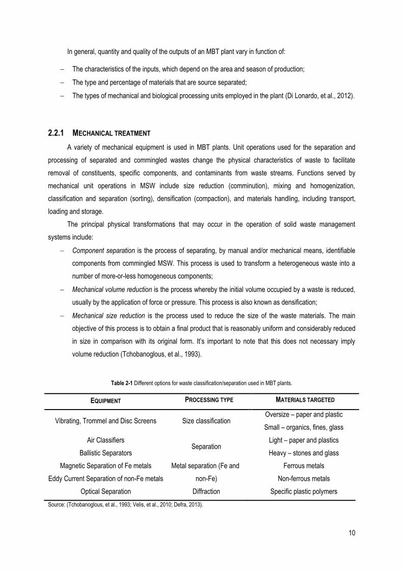
2.2.1 MECHANICAL TREATMENT
A variety of mechanical equipment is used in MBT plants. Unit operations used for the separation and
processing of separated and commingled wastes change the physical characteristics of waste to facilitate
removal of constituents, specific components, and contaminants from waste streams. Functions served by
mechanical unit operations in MSW include size reduction (comminution), mixing and homogenization,
classification and separation (sorting), densification (compaction), and materials handling, including transport,
loading and storage.
The principal physical transformations that may occur in the operation of solid waste management
systems include:
Component separation is the process of separating, by manual and/or mechanical means, identifiable
components from commingled MSW. This process is used to transform a heterogeneous waste into a
number of more-or-less homogeneous components;
Mechanical volume reduction is the process whereby the initial volume occupied by a waste is reduced,
usually by the application of force or pressure. This process is also known as densification;
Mechanical size reduction is the process used to reduce the size of the waste materials. The main
objective of this process is to obtain a final product that is reasonably uniform and considerably reduced
in size in comparison with its original form. It’s important to note that this does not necessary imply
volume reduction (Tchobanoglous, et al., 1993).
Table 2-1 Different options for waste classification/separation used in MBT plants.
EQUIPMENT PROCESSING TYPE MATERIALS TARGETED
Vibrating, Trommel and Disc Screens Size classification Oversize – paper and plastic
Small – organics, fines, glass
Air Classifiers
Ballistic Separators Separation
Light – paper and plastics
Heavy – stones and glass
Magnetic Separation of Fe metals
Eddy Current Separation of non-Fe metals
Metal separation (Fe and
non-Fe)
Ferrous metals
Non-ferrous metals
Optical Separation Diffraction Specific plastic polymers
Source: (Tchobanoglous, et al., 1993; Velis, et al., 2010; Defra, 2013).
11
Hammer mill is one of the most common types of crushing devices used to reduce the size of MSW. In
operation, material is fed into the mill by hand fed, auger or belt conveyor. Then, the hammers attached to a
rotating element, strike the waste material as it enters and eventually force the shredded material through the
discharge of the unit. Perforated metal screens or steel bar grates cover the discharge opening of the mill.
Material remains in the grinding chamber and continues to be reduced until it is able to pass through the openings
in the screen or bar grate. Finally, the result is a consistent and specific finished particle size (Tchobanoglous, et
al., 1993).
2.2.2 BIOLOGICAL TREATMENT
The principal objective of the biological treatment in MBT plant is firstly to ensure a reduction of
biodegradable waste to be disposed of in landfill in order to meet the targets of the landfill directive 99/31EC.
The main biological treatments applied to stabilize the biodegradable organic matter of solid wastes are
composting and anaerobic digestion (AD). Biological treatments may also include the both processes, aerobic
and anaerobic. Aerobic systems are in widespread use, even if anaerobic processes have the advantages of
reduced treatment time and odor emissions and it can be energetically self-sustaining due to the generation of
biogas. Aerobic processes, on the other hand, are net energy users because oxygen must be supplied for waste
conversion, but they offer the advantage of relatively simple operation, which properly operated can significantly
reduce the volume of the OFMSW (Tchobanoglous, et al., 1993; Di Lonardo, et al., 2012). In the case of AD, this
involves the degradation of organic matter in absence of oxygen by microbial organisms and leads to the
formation of biogas – a mixture of CH4 and CO2 which can be used for energy and/or heat production – and
microbial biomass (Di Lonardo, et al., 2012).
The focus was on the composting process, which will be described in detail in the following section.
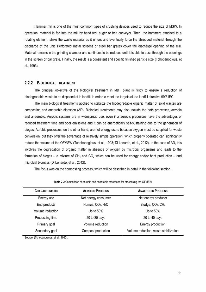
Table 2-2 Comparison of aerobic and anaerobic processes for processing the OFMSW.
CHARACTERISTIC AEROBIC PROCESS ANAEROBIC PROCESS
Energy use
End products
Volume reduction
Processing time
Primary goal
Secondary goal
Net energy consumer
Humus, CO2, H2O
Up to 50%
20 to 30 days
Volume reduction
Compost production
Net energy producer
Sludge, CO2, CH4
Up to 50%
20 to 40 days
Energy production
Volume reduction, waste stabilization
Source: (Tchobanoglous, et al., 1993).

12
2.3 COMPOSTING PROCESS
Compost quality is an important issue since compost is thought to be beneficial for both agriculture and
the environment. Like this, composting is used in solid waste management in order to convert organic waste into
a stable compost-like material that may be used to cover the landfill.
Composting can be defined as the biological decomposition and stabilization of organic substrates that
involves aerobic respiration that lead a stabilized and sanitized final product, i.e. free of pathogens and plant
seeds, known as compost, that can be beneficially applied to land (Silva & Naik, 2006). During the process,
microorganisms transform putrescible organic matter into CO2, H2O and complex metastable compounds, under
conditions that allow the development of thermophilic temperatures as a result of the heat produced by biological
reactions (Gómez & Lima, 2006). The carbon dioxide and water losses can amount to half the weight of the initial
organic materials, so composting reduces both the volume and mass of the raw materials while transforming
them into a beneficial humus-like material.
𝑂𝑟𝑔𝑎𝑛𝑖𝑐 𝑚𝑎𝑡𝑡𝑒𝑟 + 𝑂2 + 𝑛𝑢𝑡𝑟𝑖𝑒𝑛𝑡𝑠 𝑚𝑖𝑐𝑟𝑜𝑜𝑟𝑔𝑎𝑛𝑖𝑠𝑚𝑠→ 𝑛𝑒𝑤 𝑐𝑒𝑙𝑙𝑠 + 𝑐𝑜𝑚𝑝𝑜𝑠𝑡 + 𝐶𝑂2 + 𝐻2𝑂 +𝑁𝐻3
+ 𝑜𝑡ℎ𝑒𝑟 𝑔𝑎𝑠𝑒𝑠 + ℎ𝑒𝑎𝑡
2(2.1)
Table 2-3 Advantages and disadvantages of the composting process.
ADVANTAGES DISADVANTAGES
Many community wastes can be composted;
A composting facility can be designed and
operated to minimize environmental impacts;
Composting can help meet states’ landfill
reduction and recycling goals;
Composting can decompose or degrade many
organic materials;
Composting produce a usable product.
Odor and bioaerosol emissions can occur
during the process, however it can be
controlled;
Composting facilities take up more space than
some other waste management technologies;
A product must be marketed.
Source: (Epstein, 1997).
Composting is most efficient when the major parameters, like oxygen, nitrogen, carbon, moisture and
temperature, which affect the composting process, are properly managed.
The main objectives of composting process are:
To transform the biodegradable organic materials into a biologically stable material, and in the
process reduce the original volume of waste;
To destroy pathogens, insect eggs, and other unwanted organisms and weed seeds that may be
present in MSW;
13
To retain the maximum nutrient content;
To produce a product that can be used to support plant growth and as a soil amendment
(Tchobanoglous, et al., 1993).
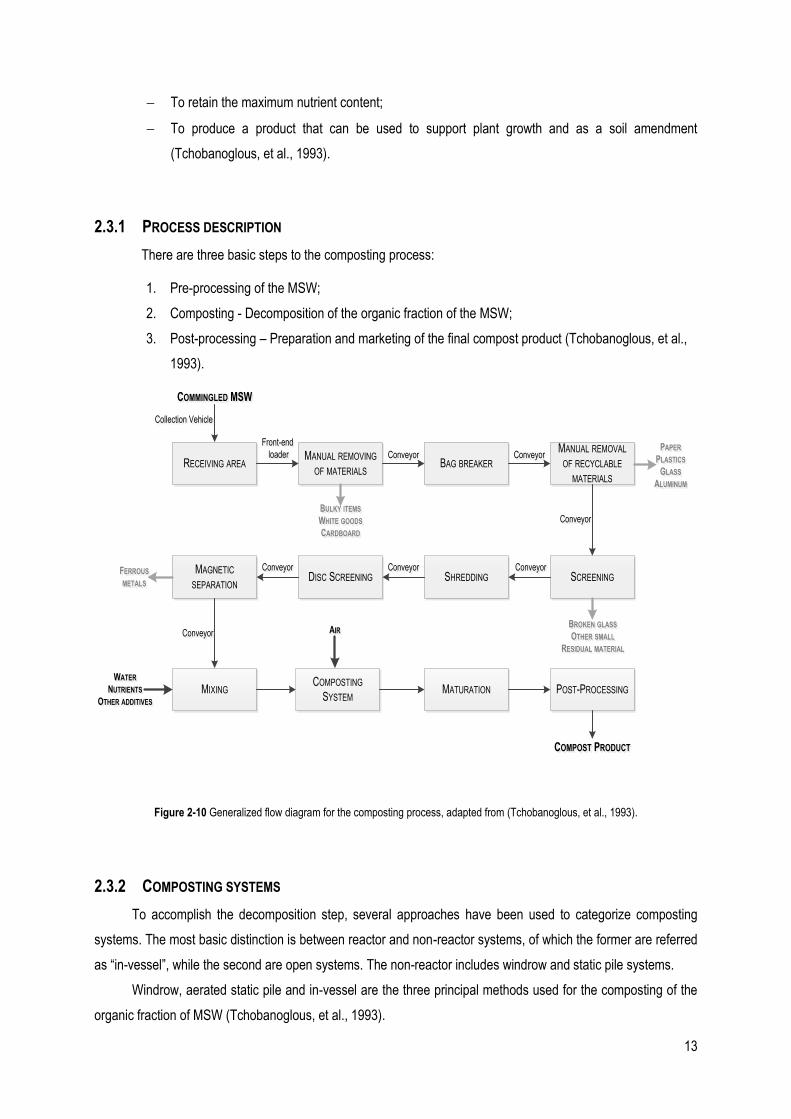
2.3.1 PROCESS DESCRIPTION
There are three basic steps to the composting process:
1. Pre-processing of the MSW;
2. Composting - Decomposition of the organic fraction of the MSW;
3. Post-processing – Preparation and marketing of the final compost product (Tchobanoglous, et al.,
1993).
RECEIVING AREAMANUAL REMOVING
OF MATERIALSBAG BREAKER
MANUAL REMOVAL
OF RECYCLABLE
MATERIALS
SCREENINGSHREDDINGDISC SCREENINGMAGNETIC
SEPARATION
MIXINGCOMPOSTING
SYSTEMMATURATION POST-PROCESSING
COMPOST PRODUCTCOMPOST PRODUCT
COMMINGLED MSWCOMMINGLED MSW
Collection VehicleCollection Vehicle
Front-end
loader
Front-end
loader ConveyorConveyor ConveyorConveyor
ConveyorConveyor
ConveyorConveyorConveyorConveyorConveyorConveyor
ConveyorConveyor AIRAIR
WATER
NUTRIENTS
OTHER ADDITIVES
WATER
NUTRIENTS
OTHER ADDITIVES
BULKY ITEMS
WHITE GOODS
CARDBOARD
BULKY ITEMS
WHITE GOODS
CARDBOARD
PAPER
PLASTICS
GLASS
ALUMINUM
PAPER
PLASTICS
GLASS
ALUMINUM
BROKEN GLASS
OTHER SMALL
RESIDUAL MATERIAL
BROKEN GLASS
OTHER SMALL
RESIDUAL MATERIAL
FERROUS
METALS
FERROUS
METALS
Figure 2-10 Generalized flow diagram for the composting process, adapted from (Tchobanoglous, et al., 1993).
2.3.2 COMPOSTING SYSTEMS
To accomplish the decomposition step, several approaches have been used to categorize composting
systems. The most basic distinction is between reactor and non-reactor systems, of which the former are referred
as “in-vessel”, while the second are open systems. The non-reactor includes windrow and static pile systems.
Windrow, aerated static pile and in-vessel are the three principal methods used for the composting of the
organic fraction of MSW (Tchobanoglous, et al., 1993).
14
2.3.2.1 WINDROW
Windrow system is the most popular method of composting. In this system, the bio-waste is laid out in
parallel rows, 2-3 m high and 3-4 m wide across the base. Windrows naturally acquire a trapezoidal shape, with
angles of repose depending on the nature of material. The actual dimensions of the windrows depend on the type
of equipment that is used to turn the material to be composted. Before forming the windrows, the material is
processed by shredding and screening is to approximately 3 to 9 cm and the moisture content is adjusted to 50-
60 %. Normally the windrows are turned up twice per week while the temperature rises to, and remains at, about
55 ºC. Complete composting is accomplished in three to four weeks. Thereafter the compost is allowed to cure
for an additional three to four weeks without turning. During this period, residual decomposable organic materials
are further reduced by fungi and actinomycetes.
As windrows are aerated primarily by natural or passive air movements, brought about convection and
gaseous diffusion, the rate of air exchange depends on the porosity of the windrow. The actual dimensions of the
windrow depend on the type of equipment that will be used to turn the composting wastes. They require large
areas of land and can cause odor problems, especially during the turning operations (Tchobanoglous, et al.,
1993).
2.3.2.2 STATIC PILE
The aerated static pile system consists of a grid of aeration or exhaust piping over which the processed
organic fraction of MSW is placed. To better control odors, piles are often covered with a textile layer. On
average aerated pile heights are about 2 to 2.5 meters. Each pile is usually provided with an individual blower for
more effective aeration control. The composting process time is about three to four weeks (Gajalakshmi &
Abbasi, 2008).
2.3.2.3 IN-VESSEL
In-vessel systems are design according to engineering principles, which help in achieving better process
efficiency, process control and optimization. These composting systems have been developed with vessels as
diverse in shapes and sizes, including vertical towers, horizontal rectangular and circular tanks, and circular
rotating tanks, only they can be divided into two major categories – plug flow and dynamic. Various forced
aeration and mechanical turning devices are used to optimize aeration in these systems. Composting periods
range from one to four weeks, though a long curing period may be necessary (about four to twelve weeks).
The increasing popularity of these composting systems is due to the process and odor control, faster
throughput, lower labor costs and smaller area requirements.
There are a variety of in-vessel methods with different combinations of vessels, turning mechanisms and
aeration devices (Tchobanoglous, et al., 1993; Gajalakshmi & Abbasi, 2008).
15
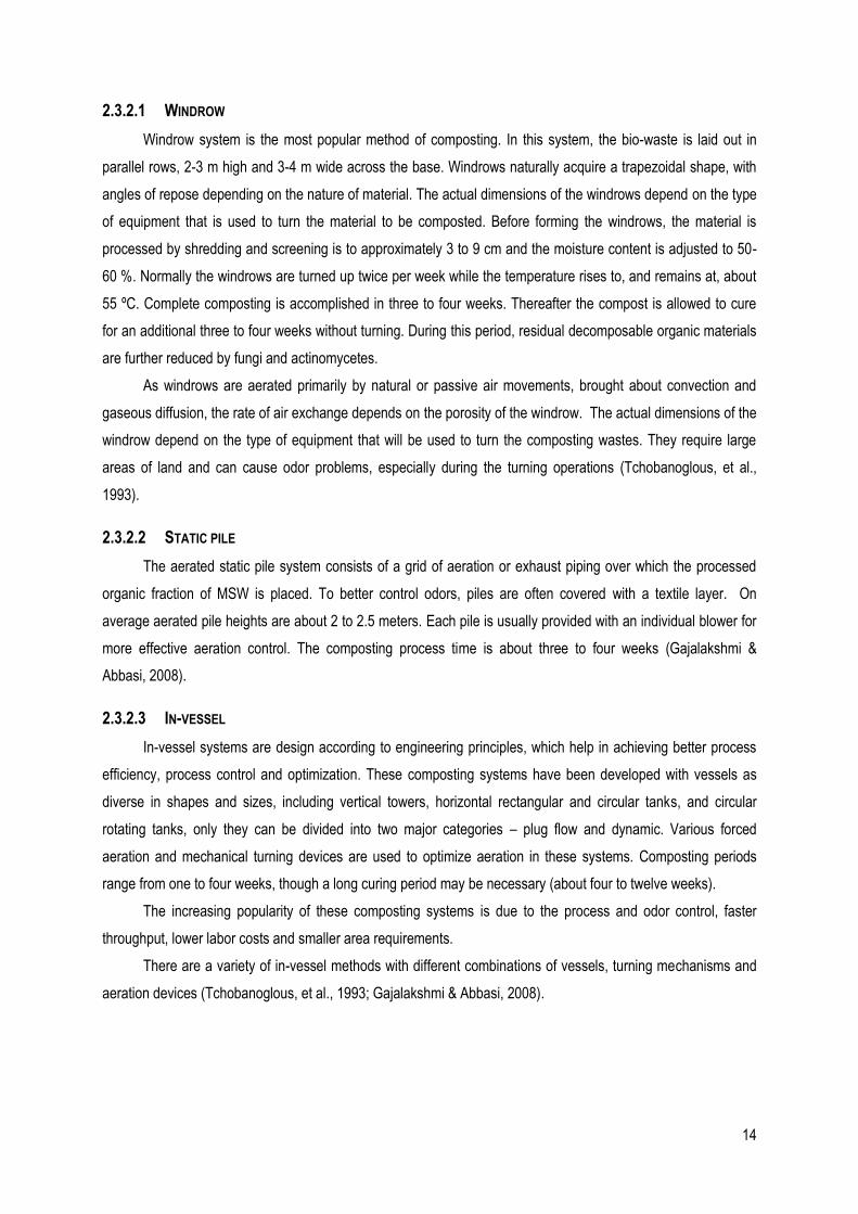
2.3.3 COMPOSTING STAGES
Composting can be divided into three stages, based on the temperature of the system:
1. A mesophilic or moderate temperature phase (10-40 ºC), which typically lasts for a couple of days;
2. A thermophilic or high temperature phase (over 40 ºC), which can last from a few days to several
months;
3. A mesophilic curing or maturation phase (10-40 ºC).
Figure 2-11 Typical temperature and pH variation during composting process-The three stages of composting, adapted from
(Trautmann & Krasny, 1997).
Mesophilic bacteria, fungi, actinomycetes and protozoa - microorganisms that function at temperatures
between 10 and 45 ºC, initiate the composting process. As a result of oxidation of carbon compounds the
temperature increases, so thermophiles – microorganisms that function at temperatures between 45 and 70 ºC,
replace the mesophilic microorganisms, which become less competitive once temperatures exceeds 40 ºC. The
thermophilic phase is the active phase of composting, wherein the process involves the degradation of easily
degradable compounds like proteins and fatty acids, resulting in the liberation of ammonium and an increase in
pH. After this, more resistant compounds such as cellulose, hemicelluloses and lignin are partly degraded. The
optimum temperature for thermophilic micro-fungi and actinomycetes which mainly degrade lignin is 40–
50˚C. Above 60˚C, these microorganisms cannot grow and lignin degradation is slowed down. As the active
16
composting phase subsides, temperature gradually declines, and mesophilic microorganisms recolonize and
the curing or maturation phase begins. During curing, organic matter continues to decompose and is
converted to biologically stable humic substances to form mature composts. The maturing phase requires
minimum oxygen and the biological activities become very slow. Once finished the process, the mature
compost may be post processed according to the feedstock characteristics and desired product quality
(Haug, 1993; Epstein, 1997).
2.3.4 CONDITIONS AND COMPONENTS AFFECTING COMPOSTING PROCESS
The period of the composting stages depends on the composition of the organic matter being composted
and the efficiency of the process, which is dependent on the control of some parameters. Composting is most
efficient when the major factors, such as temperature, moisture content, aeration, among others, which affect the
composting process are properly managed. Recently, research has been focused on the study of the interaction
between physical, chemical and biological factors, which are discussed in the following paragraphs.
2.3.4.1 NATURE OF THE SUBSTRATE
The nature of the substrate is the most basic controlling factor in any compost process, once the substrate
becomes the only source of food to the microorganisms in a compost heap. All kinds of organic residues
amenable to the enzymatic activities of the microorganisms can be converted into compost since suitable
conditions for biodegradation are provided.
The organic compounds in the bio-waste could be divided into the following fractions:
Water-soluble constituents, such as sugars, starches, amino acids, and various organic acids;
Hemicellulose, a condensation product of five and six carbon sugars;
Cellulose, a condensation product of the six carbon sugar glucose;
Fats, oils, and waxes, which are esters of alcohols and long chain fatty acids;
Lignin, a polymeric material containing aromatic rings with methoxyl groups (-OCH3);
Lignocellulose, a combination of lignin and cellulose;
Proteins, which are composed of chains of amino acids (Tchobanoglous, et al., 1993).
Most of the substrates are largely made up of polymers, which are insoluble in water. Therefore the
extracellular enzymes released by the microbes hydrolyze these polymers into monomers, which then dissolve
into water and enter the microbial cell where further decomposition takes place. If the substrate is of plant origin,
the main constituents are the carbonaceous compounds such as cellulose, hemicellulose and lignin, whereas
nitrogenous constituents (proteins) occur to a lesser extent. Protein constituents, cellulose and hemicellulose
decompose easily. Despite cellulosic substrates form good raw material for composting, lignin, requires some
attention since being a complex aromatic polymer, is resistant to microbial attack to a considerable extent.
17
However, it is not entirely recalcitrant to microbial decomposition. Basidiomycetes, a group belonging to fungi, are
well known for their ability to decompose lignin, and some bacteria and actinomycetes also possess lignolytic
characteristics (Gajalakshmi & Abbasi, 2008).
2.3.4.2 AERATION AND OXYGEN
Aeration is a key element in composting, once a large amount of oxygen is consumed, particularly, during
initial stages. Aeration provides oxygen to the aerobic organisms necessary for composting. Proper aeration is
needed to control the environmental required for biological processes to thrive with optimum efficiency. Oxygen is
not only necessary for aerobic metabolism of microorganisms, but also for oxidizing various organic molecules
present in the composting mass. If the oxygen supply is limited, the composting process might turn anaerobic,
which is a much slower and odorous process. A minimum oxygen concentration of 5% within the pore spaces of
the compost is necessary to avoid an anaerobic situation (Young, et al., 2005).
2.3.4.3 MOISTURE
Moisture is an important parameter to be controlled during composting once it influences the structural and
thermal properties of the material, as well as the rate of decomposition and metabolic process of the
microorganisms. Moisture is produced as a result of microbial activity and the biological oxidation of organic
matter, wherein water is also lost through evaporation (Epstein, 1997).
The optimum moisture content is about 60% after organic wastes have been mixed. Depending on the
components of the mixture, initial moisture content can range from 55 to 70%. However, if this exceeds 60%, the
structural strength of the compost deteriorates, oxygen movement is inhibited and the process tends to be
anaerobic. When the moisture content decreases below 50%, the rate of decomposition decreases rapidly,
whereas excessive moisture in the compost will prevent O2 diffusion to the organisms. It is important to note that
the reduction in the moisture content below 30-35% must be avoided since it causes a marked reduction in the
microbial activity. Moisture can be controlled in two ways, by adding water or indirectly by changing the operating
temperature or the aeration regime (Epstein, 1997; Young, et al., 2005).
2.3.4.4 PARTICLE SIZE
Microbial activity occurs at the interface of particle surfaces and air. Decomposition and microbial activity
will be rapid near the surfaces as oxygen diffusion is very high, so small particles have more surface area and
can degrade more quickly. Particle size also affects moisture retention as well as free air space and porosity of
the compost mixture. Aerobic decomposition increases with smaller particle size, which results in reduce air
space and less porosity, although, smaller particle size reduces the effectiveness of the oxygen supply. Optimum
composting conditions are usually obtained with particle sizes ranging from 3 to 50 mm average diameter
(Epstein, 1997; Young, et al., 2005).
2.3.4.5 POROSITY AND FREE AIR SPACE
Porosity and free air space (FAS) also have an important role in the composting process.
18
FAS is that portion of the total pore space that is not occupied with water. This parameter is intrinsically
related to the availability of water and oxygen, since pore spaces allow air to diffuse through the media and
provide oxygen to biological activity of the microorganisms (Epstein, 1997).
Porosity refers to the spaces between particles in the compost system. When the material is not saturated
with water, these spaces are partially filled with air that can supply oxygen to decomposers and provide a path for
air circulation. The more compaction and less pore space, the greater air flow resistance (Epstein, 1997).
2.3.4.6 SIZE OF COMPOST SYSTEM
The system volume requirements are an important element which must be considered in the aerobic
composting process. A compost system must be large enough to prevent rapid dissipation of heat and moisture,
yet small enough to allow good air circulation (Trautmann & Krasny, 1997).
2.3.4.7 MIXING/TURNING
Initial mixing of organic wastes is essential to increase or decrease the moisture content to an optimum
level. Mixing can be used to achieve a more uniform distribution of nutrients and microorganisms, this is to create
the interstitial spaces necessary to enable the air to flow and diffuse uniformly during the bio-oxidation stage.
Turning of the organic material during the composting process is a important operational factor in maintaining
aerobic activity (Tchobanoglous, et al., 1993).
2.3.4.8 TEMPERATURE
Temperature plays a major role in composting process. Probably it is the most important parameter
affecting microbial activity, and variations in temperature affect the various stages of composting. Temperature is
produced during the composting process, resulting from the breakdown of organic matter by microbes (Epstein,
1997).
The temperature can range from near freezing to 70 ºC. Starting at ambient temperature when the
components are mixed, the compost can reach 40-60 ºC in fewer two days depending on the composition and
environmental conditions. Temperature is also a good indicator of the various stages of the composting process,
which is divided into four phases based on it. The first is the mesophilic stage, where mesophilic organisms
generate large quantities of metabolic heat and energy due to availability of abundant nutrients, but gradually this
will pave the way for the dominance of thermophiles, for several days or weeks. With depletion of food sources,
overall microbial activity decreases and temperature falls to ambient, leading to the second mesophilic stage,
where microbial growth will be slower as readily available food is consumed. Finally, compost material enters the
maturation stage, which might take some months (Young, et al., 2005).
It is important to note that for destroying pathogenic microorganisms the temperature should reach at
least 55 to 65 °C for some hours to a few days (Gajalakshmi & Abbasi, 2008).
19
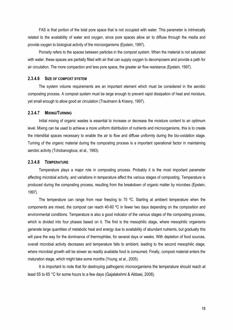
Table 2-4 Temperature and the Time Interval Required to Destroy Most Common Types of Pathogenic Microorganisms and Parasites.
PATHOGEN TEMPERATURE AND TIME
Salmonella typhosa Further growth is stopped above 46ºC; dies within 20–30 minutes at temperature of 55–60ºC.
Salmonella sp. Dies within 60 and 20 minutes at a temperature of 55 and 60ºC, respectively.
Shigella sp. Dies within 60 and 20 minutes at a temperature of 55ºC.
Escherichia coli Most of it dies within 60 and 20 minutes at a temperature of 55 and 60ºC,
respectively.
Source: (Tchobanoglous, et al., 1993; Gajalakshmi & Abbasi, 2008).
2.3.4.9 NUTRIENTS
The microorganisms that carry out the composting process require a variety of nutrients for their growth,
which can be classified into macro and micro nutrients, according to the amounts in which they are needed by
microorganisms. The major nutrients of concern are the macro nutrients nitrogen and phosphorous, and the micro
nutrients such as iron, calcium, and magnesium (Haug, 1993).
During composting, the most common nutrient limitations are related with nitrogen, which is discussed in
more detail in following section.
2.3.4.10 CARBON-TO-NITROGEN RATIO
The two most important nutrients are C and N, whose ratios affect the process and the product. Carbon
provides the preliminary energy source and nitrogen quantity determines the microbial population growth.
Therefore, maintaining the correct C/N ratio is important to obtain good quality compost. During microbial growth,
approximately 25 to 30 parts of C are needed for every unit of N. Composting is usually successful when the
mixture of organic materials consists of 20-40 parts of C to 1 part of N. Nevertheless, as the ratio exceed 30, the
rate of composting decreases, further, as the ratio decreases below 25, excess nitrogen is volatilized in the form
of ammonia. This is released into the atmosphere and results in undesirable odor (Epstein, 1997; Young, et al.,
2005).
During bioconversation of the materials, concentration of carbon will be reduced while that of nitrogen will
be increased, resulting in the reduction of C/N ratio at the end of the compost process. This reduction can be
attributed to the loss in total dry mass due to losses of C as CO2. NH4-N and NO3-N will also undergo some
changes. NH3 levels were increasing in the initial stages but declining towards the end. In several instances, NO3
concentrations were less during the initial phases but gradually increased towards in the end, wherein some
instances, remained unchanged. Maintaining NH3 concentration is important to avoid excess nitrogen losses and
production of bad odor (Epstein, 1997; Young, et al., 2005; Gajalakshmi & Abbasi, 2008).
2.3.4.11 PH
Control of pH is another important parameter that greatly affects the composting process. During the
course of composting, the pH generally varies between 5.5 and 8.5. The initial pH of the organic fraction of MSW
is typically between 5 and 7. In the first few days of composting, the pH drop to 5 or less. The resulting drop in pH
20
encourages the growth of fungi, which are active in the decomposition of lignin and cellulose. Usually, the organic
acids break down further during the composting process, and the pH begins to rise to approximately 8 or 8.5. This
is caused by two processes that occur during the thermophilic stage – decomposition and volatilization of organic
acids, and release of ammonia by microbes as they break down proteins and other nitrogen sources. The pH falls
slightly during the cooling stage and reaches to a value in the range of 7 to 8 in the mature compost. If the degree
of aeration is not adequate, it will not follow this trend, once anaerobic conditions will occur, the pH will drop to
about 4.5, limiting microbial activity and the composting process will be retarded (Tchobanoglous, et al., 1993;
Trautmann & Krasny, 1997).
2.3.4.12 ODOR
The majority of odor problems in aerobic composting processes are associated with the development of
anaerobic conditions, in which organic acids, extremely odorous, will be produced. To minimize the potential odor
problems, it is important to reduce the particle size, remove plastic and other non-biodegradable matter from the
organic material to be composted (Tchobanoglous, et al., 1993).
2.3.4.13 MICROORGANISMS
Composting involves innumerable microorganisms. The composition and magnitude of these
microorganisms are important components of the composting process. The microorganisms decompose organic
materials, and transform the nitrogen component through oxidation, nitrification and denitrification. Composting
may also involve sequential growth and degradations of subpopulations.
Microorganisms cannot directly metabolize the insoluble particles of organic matter. However, the
microbes produce hydrolytic enzymes to depolymerize the larger compounds to smaller fragments that are
soluble in water (Epstein, 1997; Gajalakshmi & Abbasi, 2008).
Bacteria play by far the most dominant role during the most active stages of composting process due of
their ability to grow rapidly on soluble proteins and other readily available substrates, and they may also attack
more complex materials. Among bacteria that occur commonly in aerobically decomposing substrate are species
of Bacillus. Clostridium occurs substantially in anaerobic conditions (Gajalakshmi & Abbasi, 2008).
The role of fungi starts when simple, easily degradable substances such as sugar, starch, and protein are
acted upon by bacteria and the substrate is predominated by cellulose and lignin, which normally occurs toward
the later stages of composting. Most fungi are eliminated by high temperatures, yet they commonly recover when
temperatures are moderate. Fungi build up much higher biomass than other microorganisms, once they are
efficient consumers of carbon (Epstein, 1997; Gajalakshmi & Abbasi, 2008).
The actinomycetes are a group of organisms with intermediate properties between bacteria and fungi. Like
fungi, actinomycetes also use complex organic matter. They tend to show their activity in the later stages of
decomposition. The actinomycetes that occur most frequently are Microbispora, Streptomyces and
Thermoactinomyces (Tchobanoglous, et al., 1993; Gajalakshmi & Abbasi, 2008).
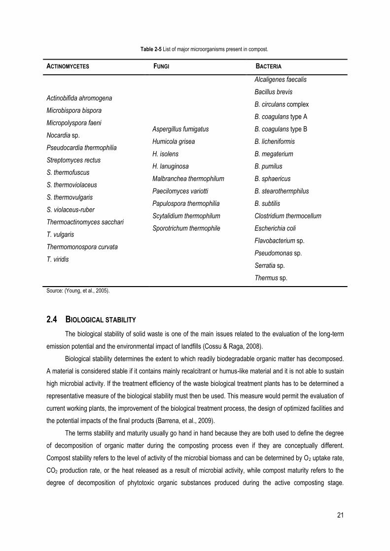
21
Table 2-5 List of major microorganisms present in compost.
ACTINOMYCETES FUNGI BACTERIA
Actinobifida ahromogena
Microbispora bispora
Micropolyspora faeni
Nocardia sp.
Pseudocardia thermophilia
Streptomyces rectus
S. thermofuscus
S. thermoviolaceus
S. thermovulgaris
S. violaceus-ruber
Thermoactinomyces sacchari
T. vulgaris
Thermomonospora curvata
T. viridis
Aspergillus fumigatus
Humicola grisea
H. isolens
H. lanuginosa
Malbranchea thermophilum
Paecilomyces variotti
Papulospora thermophilia
Scytalidium thermophilum
Sporotrichum thermophile
Alcaligenes faecalis
Bacillus brevis
B. circulans complex
B. coagulans type A
B. coagulans type B
B. licheniformis
B. megaterium
B. pumilus
B. sphaericus
B. stearothermphilus
B. subtilis
Clostridium thermocellum
Escherichia coli
Flavobacterium sp.
Pseudomonas sp.
Serratia sp.
Thermus sp.
Source: (Young, et al., 2005).
2.4 BIOLOGICAL STABILITY
The biological stability of solid waste is one of the main issues related to the evaluation of the long-term
emission potential and the environmental impact of landfills (Cossu & Raga, 2008).
Biological stability determines the extent to which readily biodegradable organic matter has decomposed.
A material is considered stable if it contains mainly recalcitrant or humus-like material and it is not able to sustain
high microbial activity. If the treatment efficiency of the waste biological treatment plants has to be determined a
representative measure of the biological stability must then be used. This measure would permit the evaluation of
current working plants, the improvement of the biological treatment process, the design of optimized facilities and
the potential impacts of the final products (Barrena, et al., 2009).
The terms stability and maturity usually go hand in hand because they are both used to define the degree
of decomposition of organic matter during the composting process even if they are conceptually different.
Compost stability refers to the level of activity of the microbial biomass and can be determined by O2 uptake rate,
CO2 production rate, or the heat released as a result of microbial activity, while compost maturity refers to the
degree of decomposition of phytotoxic organic substances produced during the active composting stage.
22
Compost stability is strongly related to the rate of microbial activity in the compost, and compost maturity is used
to describe product quality (Gajalakshmi & Abbasi, 2008).
The utilization of methods for the assessment of the biological stability of waste has been increasingly
common with different aims, such as:
Monitoring of the effectiveness of the biological degradation process during high quality compost
production from the separately collected biodegradable organic fraction of municipal solid waste
(OFMSW) or from other biodegradable waste;
Evaluation of the reduction of biological activity of solid waste as a result of aerobic or anaerobic
stabilization processes before disposal in landfill;
Monitoring of the effects of in situ aeration processes on the deposited waste for old landfill remediation;
Evaluation of the effects of the aerobic conditions in innovate aerobic or semi-aerobic landfills;
Evaluation of the emission potential of deposited waste in old landfills in view of possible remediation
(Cossu & Raga, 2008).
2.4.1 RESPIROMETRIC METHODS
The use of a respiration index has become popular around the Europe, and numerous authors have
considered it for waste characterization (Cossu & Raga, 2008).
Respiration can be considered as a general measure of the microbial activity. It can provide a reliable,
repeatable and scientifically sound assessment of microbial activity. For this reason, and despite the various
methods that have been proposed in the past, the respirometric test is recognized as being the best method to
measure microbial activity and therefore, stability of a compost (Adani, et al., 2006; Gómez & Lima, 2006).
Oxygen is consumed and carbon dioxide is evolved as a consequence of microbial metabolism. Both the
processes decline at late composting stages. Insufficiently mature compost has a strong demand for O2 and high
CO2 production rates due to intense development of microorganisms as a consequence of the abundance of
easily biodegradable compounds in the substrate. The method of determination of the respiration activity serves
the purpose of assessment of the biological reactivity or the degree of maturity of the stabilized materials in
aerobic conditions. It determines the quantity of oxygen used by microorganisms during a specific time under
laboratory conditions. This way, the oxygen demand may be specified by the measurement of the quantity of
consumed oxygen or produced carbon dioxide and is expressed in g O2/kg of dry mass of waste (Myszograj, et
al., 2014).
Actually, the respiration indices are regarded as the key parameters which serve the purpose of
assessment of the compost stability and hence, its quality.
Respirometric methods can be used to determine the biological activity in a sample if the assay is
performed under optimal and controlled conditions. As already mentioned for composting process, also
respirometric assays are affected by many different factors such as moisture content, temperature of the sample,
microbial population, nutrients equilibrium, or occurrence of toxic compounds (Gómez & Lima, 2006).

23
2.4.1.1 SELF-HEATING TEST
The self-heating test measures the temperature increase due to the heat released from the biological and
chemical activity of a compost sample. This method is simple to implement and results are easy to understand,
and is widely used in Europe. However, this test cannot be directly correlated to respiration since many chemical
and biochemical reactions not related to respiration are also exothermal. In addition, biomass heating is also
influenced by other factors such as porosity or moisture content. Nevertheless, in previous studies, the
respirometric activity of a compost sample was indirectly determined from results obtained in a self-heating test
using a bio-energy approach to estimate the heat generated along the process (Gómez & Lima, 2006).
2.4.1.2 METHODS BASED ON CO2 PRODUCTION
These methods are widely used in commercial laboratories, and their equipment is generally very simple
and easy to use. CO2 production is directly correlated with the aerobic respiration. Among the most commonly
used are those that use alkaline traps to fix the CO2. The main disadvantage of these methods is that they are
unable to distinguish between CO2 produced aerobically from that produced anaerobically. Moreover, these
methods assume that the CO2/O2 ratio is always one. Monitoring of CO2 evolution presents two major drawbacks:
the solubility of CO2 in aqueous solutions and this solubility is pH dependent. This is important when comparing
respiration activities of different residues since their pH can vary over a wide range (Myszograj, et al., 2014).
2.4.1.3 METHODS BASED ON O2 UPTAKE
These are the most accepted methods for the determination of the biological activity of a material, once
they provide accurate information on the activity of a compost sample. Nevertheless, their main disadvantage is
that they need more specific instrumentation and skilled labor. In addition, the equipment needs constant
maintenance and frequent calibration (Gómez & Lima, 2006).
Methods based on O2 uptake rate have been classified into to different classes: static (SRT) and dynamic
(DRT) respiration tests. Static tests are performed at the absence of continuous airflow and O2 consumption is
usually measured via pressure differences or via direct measurements of the O2 content in air or liquid medium.
They can be performed either with solid or liquid samples. Dynamic tests are continuous air flow systems which
allow oxygen transfer through the biomass layers to cells. This is important, since it minimize O2 diffusion
limitations, which are frequent in solid substrates. These dynamic tests require the precise measurement of
airflow rate throughout the process and the measurement of O2 and CO2 contents at the inlet and outlet of the test
devices (Gómez & Lima, 2006; Komilis, et al., 2011; Komilis & Kanellos, 2012).
The SOUR (specific oxygen uptake rate) test utilizes a dissolved oxygen probe to measure changes in the
oxygen concentration of an aqueous compost suspension. The OD20 (oxygen demand) is calculated from the
integration of the oxygen uptake curve from 0 to 20 hours. The DSOUR (dry specific oxygen uptake rate)
measures changes in O2 concentration in the head space of a closed flask containing a moist compost sample of
known volume and mass, at known temperature and barometric pressure. The decline in oxygen concentration
24
over time is monitored with an O2 electrode (Lasardi & Stentiford, 1998; Gómez & Lima, 2006). The DRI (dynamic
respiration index) is determined measuring the difference in O2 concentration between the inlet and outlet of an
airflow passing throughout a compost reactor. According to the assay conditions Adani et al. (2001) distinguish
between a real DRI (RDRI) carried out with no moisture adjustment of the sample a potential DRI (PDRI) for
samples adjusted to optimal moisture. The static respiration index (SRI) can also be estimated in the same
reactor, however, aeration is stopped and an O2 electrode is placed in the headspace on top of the solid material.
O2 uptake rate is calculated from the decline in O2 concentration (Adani, et al., 2001; Gómez & Lima, 2006). AT4
and AT7 were suggested by Binner et al. (1998) and they measure the respiration activity after 4 and 7 days,
respectively. For these tests are used two different respirometric systems – Sapromat® and OxiTop®. Although
Sapromat® has many advantages during the last years OxiTop® got more common (Binner & Zach, 1998; Binner,
et al., 2012).
Table 2-6 summarizes the characteristics of the main respirometric methods.
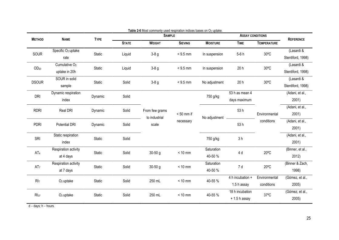
25
Table 2-6 Most commonly used respiration indices bases on O2 uptake.
METHOD NAME TYPE SAMPLE ASSAY CONDITIONS
REFERENCE STATE WEIGHT SIEVING MOISTURE TIME TEMPERATURE
SOUR Specific O2 uptake
rate Static Liquid 3-8 g < 9.5 mm In suspension 5-6 h 30ºC
(Lasardi &
Stentiford, 1998)
OD20 Cumulative O2
uptake in 20h Static Liquid 3-8 g < 9.5 mm In suspension 20 h 30ºC
(Lasardi &
Stentiford, 1998)
DSOUR SOUR in solid
sample Static Solid 3-8 g < 9.5 mm No adjustment 20 h 30ºC
(Lasardi &
Stentiford, 1998)
DRI Dynamic respiration
index Dynamic Solid
From few grams
to industrial
scale
< 50 mm if
necessary
750 g/kg 53 h as mean 4
days maximum
Environmental
conditions
(Adani, et al.,
2001)
RDRI Real DRI Dynamic Solid
No adjustment
53 h (Adani, et al.,
2001)
PDRI Potential DRI Dynamic Solid 53 h (Adani, et al.,
2001)
SRI Static respiration
index Static Solid 750 g/kg 3 h
(Adani, et al.,
2001)
AT4 Respiration activity
at 4 days Static Solid 30-50 g < 10 mm
Saturation
40-50 % 4 d 20ºC
(Binner, et al.,
2012)
AT7 Respiration activity
at 7 days Static Solid 30-50 g < 10 mm
Saturation
40-50 % 7 d 20ºC
(Binner & Zach,
1998)
RIT O2 uptake Static Solid 250 mL < 10 mm 40-55 % 4 h incubation +
1.5 h assay
Environmental
conditions
(Gómez, et al.,
2005)
RI37 O2 uptake Static Solid 250 mL < 10 mm 40-55 % 18 h incubation
+ 1.5 h assay 37ºC
(Gómez, et al.,
2005)
d – days; h – hours.
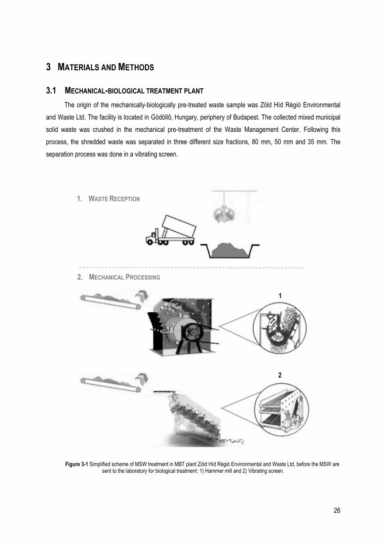
26
3 MATERIALS AND METHODS
3.1 MECHANICAL-BIOLOGICAL TREATMENT PLANT
The origin of the mechanically-biologically pre-treated waste sample was Zöld Híd Régió Environmental
and Waste Ltd. The facility is located in Gödöllő, Hungary, periphery of Budapest. The collected mixed municipal
solid waste was crushed in the mechanical pre-treatment of the Waste Management Center. Following this
process, the shredded waste was separated in three different size fractions, 80 mm, 50 mm and 35 mm. The
separation process was done in a vibrating screen.
Figure 3-1 Simplified scheme of MSW treatment in MBT plant Zöld Híd Régió Environmental and Waste Ltd, before the MSW are sent to the laboratory for biological treatment: 1) Hammer mill and 2) Vibrating screen.
1. WASTE RECEPTION
2. MECHANICAL PROCESSING
1
2
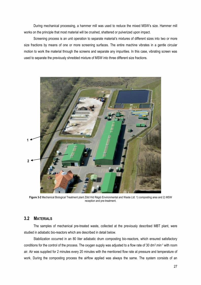
27
During mechanical processing, a hammer mill was used to reduce the mixed MSW’s size. Hammer mill
works on the principle that most material will be crushed, shattered or pulverized upon impact.
Screening process is an unit operation to separate material’s mixtures of different sizes into two or more
size fractions by means of one or more screening surfaces. The entire machine vibrates in a gentle circular
motion to work the material through the screens and separate any impurities. In this case, vibrating screen was
used to separate the previously shredded mixture of MSW into three different size fractions.
Figure 3-2 Mechanical Biological Treatment plant Zöld Híd Régió Environmental and Waste Ltd: 1) composting area and 2) MSW reception and pre-treatment.
3.2 MATERIALS
The samples of mechanical pre-treated waste, collected at the previously described MBT plant, were
studied in adiabatic bio-reactors which are described in detail below.
Stabilization occurred in an 80 liter adiabatic drum composting bio-reactors, which ensured satisfactory
conditions for the control of the process. The oxygen supply was adjusted to a flow rate of 30 dm3.min-1 with room
air. Air was supplied for 2 minutes every 20 minutes with the mentioned flow rate at pressure and temperature of
work. During the composting process the airflow applied was always the same. The system consists of an
1
2
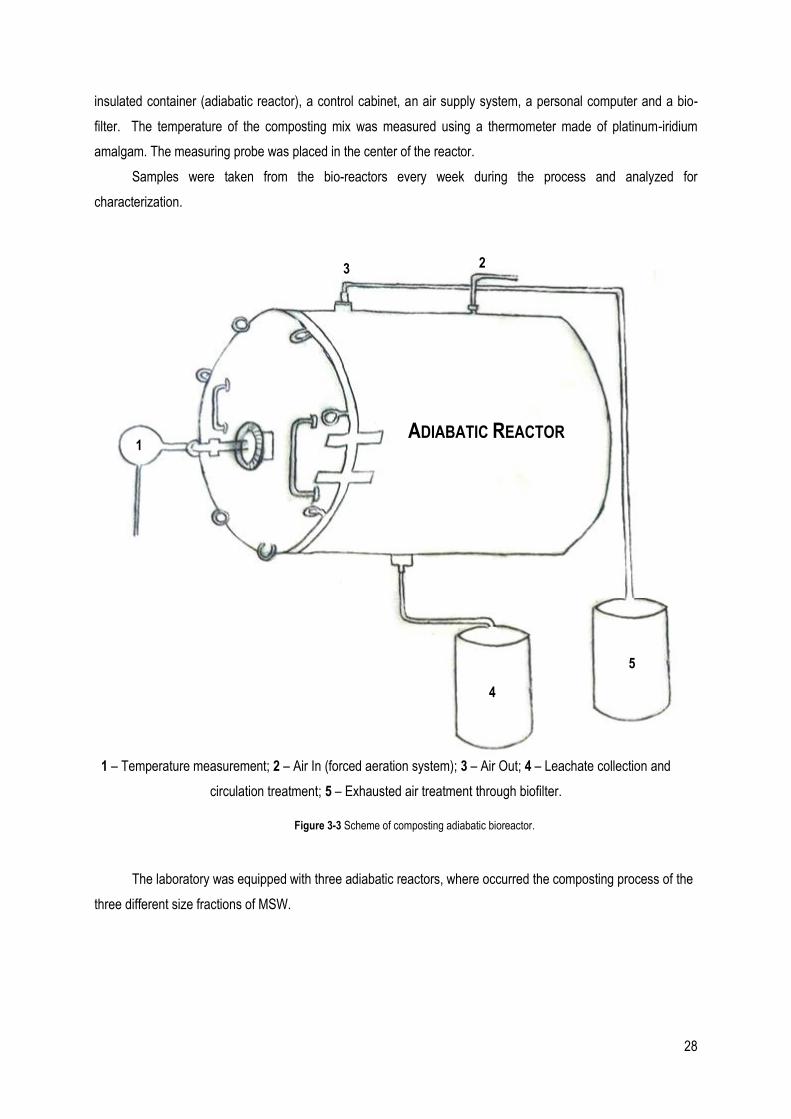
28
insulated container (adiabatic reactor), a control cabinet, an air supply system, a personal computer and a bio-
filter. The temperature of the composting mix was measured using a thermometer made of platinum-iridium
amalgam. The measuring probe was placed in the center of the reactor.
Samples were taken from the bio-reactors every week during the process and analyzed for
characterization.
Figure 3-3 Scheme of composting adiabatic bioreactor.
The laboratory was equipped with three adiabatic reactors, where occurred the composting process of the
three different size fractions of MSW.
1
2 3
4
5
ADIABATIC REACTOR
1 – Temperature measurement; 2 – Air In (forced aeration system); 3 – Air Out; 4 – Leachate collection and
circulation treatment; 5 – Exhausted air treatment through biofilter.
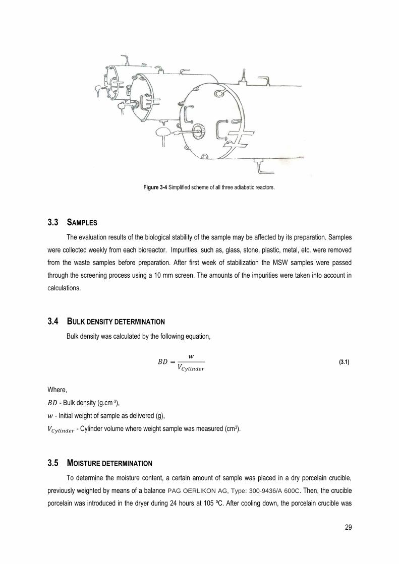
29
Figure 3-4 Simplified scheme of all three adiabatic reactors.
3.3 SAMPLES
The evaluation results of the biological stability of the sample may be affected by its preparation. Samples
were collected weekly from each bioreactor. Impurities, such as, glass, stone, plastic, metal, etc. were removed
from the waste samples before preparation. After first week of stabilization the MSW samples were passed
through the screening process using a 10 mm screen. The amounts of the impurities were taken into account in
calculations.
3.4 BULK DENSITY DETERMINATION
Bulk density was calculated by the following equation,
𝐵𝐷 =𝑤
𝑉𝐶𝑦𝑙𝑖𝑛𝑑𝑒𝑟
(3.1)
Where,
𝐵𝐷 - Bulk density (g.cm-3),
𝑤 - Initial weight of sample as delivered (g),
𝑉𝐶𝑦𝑙𝑖𝑛𝑑𝑒𝑟 - Cylinder volume where weight sample was measured (cm3).
3.5 MOISTURE DETERMINATION
To determine the moisture content, a certain amount of sample was placed in a dry porcelain crucible,
previously weighted by means of a balance PAG OERLIKON AG, Type: 300-9436/A 600C. Then, the crucible
porcelain was introduced in the dryer during 24 hours at 105 ºC. After cooling down, the porcelain crucible was
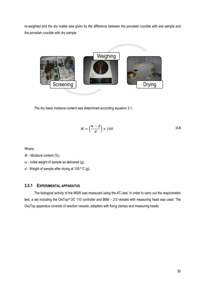
30
re-weighted and the dry matter was given by the difference between the porcelain crucible with wet sample and
the porcelain crucible with dry sample.
The dry basis moisture content was determined according equation 3.1,
𝑀 = (𝑤 − 𝑑
𝑑) × 100
(3.2)
Where,
𝑀 - Moisture content (%),
𝑤 - Initial weight of sample as delivered (g),
𝑑 - Weight of sample after drying at 105 º C (g).
3.5.1 EXPERIMENTAL APPARATUS
The biological activity of the MSW was measured using the AT4 test. In order to carry out the respirometric
test, a set including the OxiTop® OC 110 controller and B6M – 2.5 vessels with measuring head was used. The
OxyTop apparatus consists of reaction vessels, adapters with fixing clamps and measuring heads.
Screening
Weighing
Drying
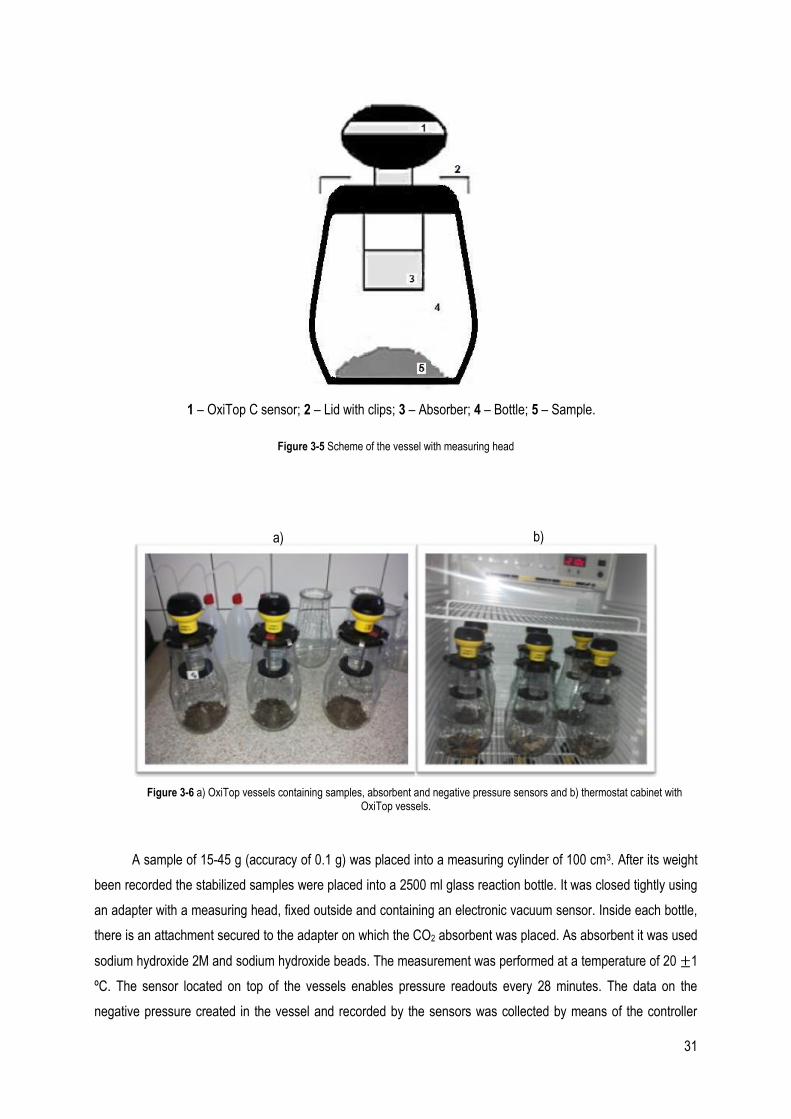
31
Figure 3-5 Scheme of the vessel with measuring head
Figure 3-6 a) OxiTop vessels containing samples, absorbent and negative pressure sensors and b) thermostat cabinet with OxiTop vessels.
A sample of 15-45 g (accuracy of 0.1 g) was placed into a measuring cylinder of 100 cm3. After its weight
been recorded the stabilized samples were placed into a 2500 ml glass reaction bottle. It was closed tightly using
an adapter with a measuring head, fixed outside and containing an electronic vacuum sensor. Inside each bottle,
there is an attachment secured to the adapter on which the CO2 absorbent was placed. As absorbent it was used
sodium hydroxide 2M and sodium hydroxide beads. The measurement was performed at a temperature of 20 ±1
ºC. The sensor located on top of the vessels enables pressure readouts every 28 minutes. The data on the
negative pressure created in the vessel and recorded by the sensors was collected by means of the controller
1 – OxiTop C sensor; 2 – Lid with clips; 3 – Absorber; 4 – Bottle; 5 – Sample.
a) b)
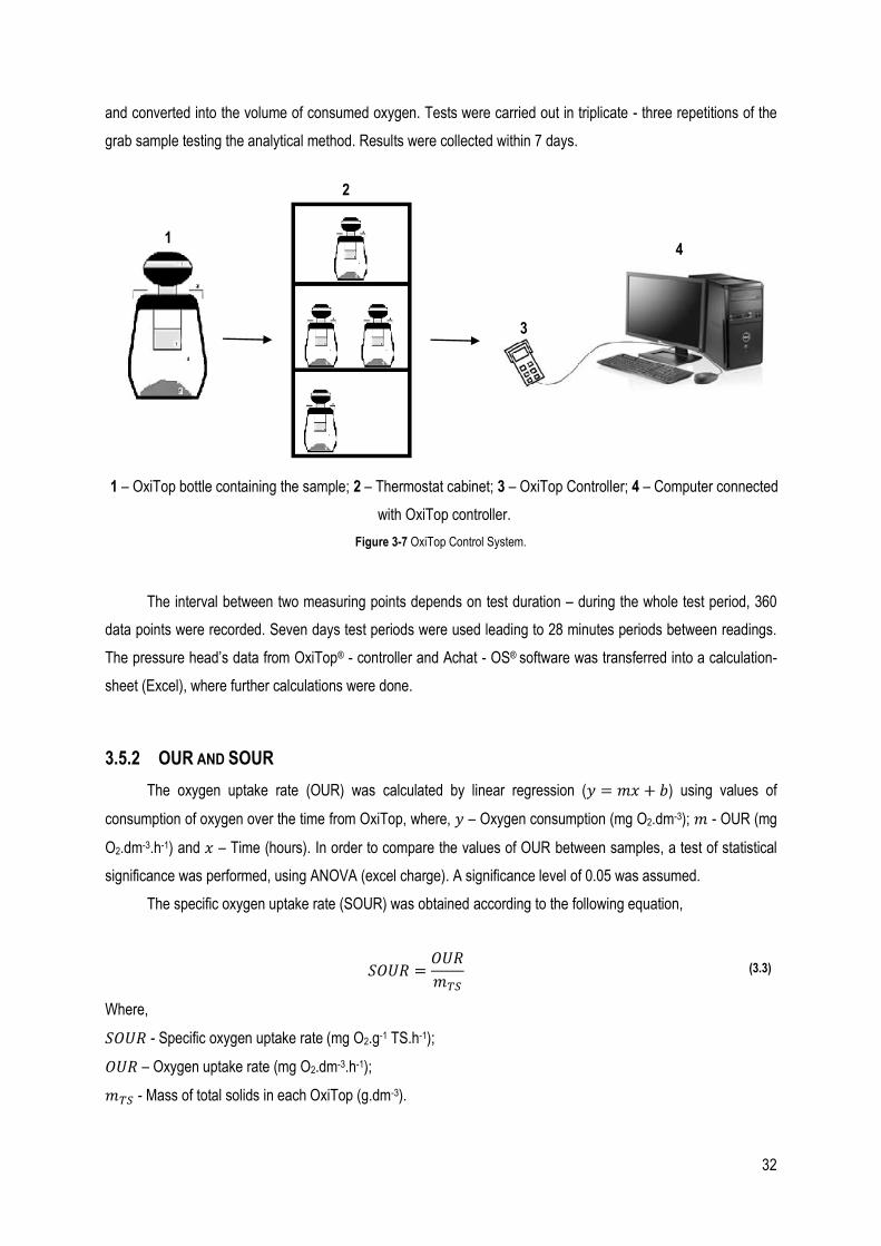
32
and converted into the volume of consumed oxygen. Tests were carried out in triplicate - three repetitions of the
grab sample testing the analytical method. Results were collected within 7 days.
Figure 3-7 OxiTop Control System.
The interval between two measuring points depends on test duration – during the whole test period, 360
data points were recorded. Seven days test periods were used leading to 28 minutes periods between readings.
The pressure head’s data from OxiTop® - controller and Achat - OS® software was transferred into a calculation-
sheet (Excel), where further calculations were done.
3.5.2 OUR AND SOUR
The oxygen uptake rate (OUR) was calculated by linear regression (𝑦 = 𝑚𝑥 + 𝑏) using values of
consumption of oxygen over the time from OxiTop, where, 𝑦 – Oxygen consumption (mg O2.dm-3); 𝑚 - OUR (mg
O2.dm-3.h-1) and 𝑥 – Time (hours). In order to compare the values of OUR between samples, a test of statistical
significance was performed, using ANOVA (excel charge). A significance level of 0.05 was assumed.
The specific oxygen uptake rate (SOUR) was obtained according to the following equation,
𝑆𝑂𝑈𝑅 =𝑂𝑈𝑅
𝑚𝑇𝑆 (3.3)
Where,
𝑆𝑂𝑈𝑅 - Specific oxygen uptake rate (mg O2.g-1 TS.h-1);
𝑂𝑈𝑅 – Oxygen uptake rate (mg O2.dm-3.h-1);
𝑚𝑇𝑆 - Mass of total solids in each OxiTop (g.dm-3).
1
2
3
4
1 – OxiTop bottle containing the sample; 2 – Thermostat cabinet; 3 – OxiTop Controller; 4 – Computer connected
with OxiTop controller.
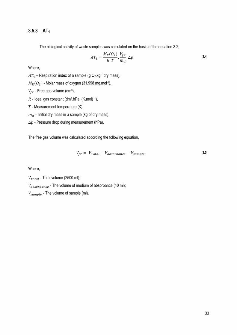
33
3.5.3 AT4
The biological activity of waste samples was calculated on the basis of the equation 3.2,
𝐴𝑇4 =𝑀𝑅(𝑂2)
𝑅. 𝑇.𝑉𝑓𝑟
𝑚𝑑. ∆𝑝 (3.4)
Where,
𝐴𝑇4 – Respiration index of a sample (g O2.kg-1 dry mass),
𝑀𝑅(𝑂2) - Molar mass of oxygen (31,998 mg.mol-1),
𝑉𝑓𝑟 - Free gas volume (dm3),
𝑅 - Ideal gas constant (dm3.hPa. (K.mol) -1),
𝑇 - Measurement temperature (K),
𝑚𝑑 – Initial dry mass in a sample (kg of dry mass),
∆𝑝 - Pressure drop during measurement (hPa).
The free gas volume was calculated according the following equation,
𝑉𝑓𝑟 = 𝑉𝑇𝑜𝑡𝑎𝑙 − 𝑉𝑎𝑏𝑠𝑜𝑟𝑏𝑎𝑛𝑐𝑒 − 𝑉𝑠𝑎𝑚𝑝𝑙𝑒
(3.5)
Where,
𝑉𝑇𝑜𝑡𝑎𝑙 - Total volume (2500 ml);
𝑉𝑎𝑏𝑠𝑜𝑟𝑏𝑎𝑛𝑐𝑒 - The volume of medium of absorbance (40 ml);
𝑉𝑠𝑎𝑚𝑝𝑙𝑒 - The volume of sample (ml).

34
4 RESULTS AND DISCUSSION
In this chapter, it is shown the relevant data obtained in the characterization of the biological stability of
the municipal solid waste during the biological process by means of respiration activity.
4.1 MOISTURE
The appropriate moisture content (MC) of the sample has a significant impact on the obtained results. The
MC of solid wastes usually is expressed in one of two ways – wet weight method or dry weigh method. In the first
one the moisture in a sample is expressed as a percentage of the wet weight of the material while in the second
one it is expressed as a percentage of the dry weight of the material (Tchobanoglous, et al., 1993).
First, the moisture content was calculated for a sample without biological stabilization treatment (week 0).
During the composting process the samples were taken on a weekly basis.
The grab samples were collected and the moisture measurement was performed at room temperature.
Values of moisture content are represented in table 4-1 and Figure 4-1.
Table 4-1 Moisture content in dry basis for each MSW fraction at the end of each week of biological stabilization, at room temperature. The results are average (N=3).
WEEKS MOISTURE CONTENT (%)
35 mm 50 mm 80 mm
0 62.8 72.2 77.4
1 59.0 71.7* 78.2*
2 39.9* 47.5* 69.2
3 45.9** - 64.8*
4 39.5 66.2* 61.8
* The results are average (N=2);
**The result is from a single sample (without repetitions).
An excessively small quantity of water does not ensure optimal conditions for the development of
microorganisms to process the given material. Nevertheless, excessive water content causes the pores inside the
material to become clogged which prevents the air from free circulation (Myszograj, et al., 2014).
For a MSW fraction of 35 mm, composting process started with moisture content of about 60%. According
to various authors it is considered ideal to start with. The same fraction had a decrease of moisture content over
the stabilization time by checking only a slightly increase at the end of third week of treatment.
Relative to the MSW fraction of 50 mm, composting process started with moisture content of about 70%
and it decreases until 66.2% over the stabilization time.
Finally for MSW fraction of 80 mm, composting began with 77.4% moisture content and it decreases till
61.8% at the end of stabilization time.

35
4.2 TEMPERATURE
Temperature is an important parameter affecting microbial activity, and variations in temperature affecting
the various phases of composting (Young, et al., 2005).
During the time of biological stabilization, temperature was measured in the three different reactors. The
temperature profiles obtained during the composting process are illustrated in figure 4-1.

36
Figure 4-1 Relationship between the temperature, measured during the composting process in the bio-reactors with a 30dm3.min-1 air flow provided for 2 minutes every 20 minutes , and moisture measured at the end of each week of biological stabilization at room temperature.
a) MSW fraction of 35 mm; b) MSW fraction of 50 mm and c) MSW fraction of 80 mm.
10
20
30
40
50
60
70
80
10
20
30
40
50
60
70
80
0 4 8 12 16 20 24 28
Mo
istu
re (
%)
Tem
per
atu
re (
ºC)
Time (days)
10
20
30
40
50
60
70
80
90
10
20
30
40
50
60
70
80
0 4 8 12 16 20 24 28
Mo
istu
re (
%)
Tem
per
atu
re (
ºC)
Time (days)
10
20
30
40
50
60
70
80
10
20
30
40
50
60
70
80
0 4 8 12 16 20 24 28
Mo
istu
re (
%)
Tem
per
atu
re (
ºC)
Time (days)
Temperature Moisture
a)
b)
c)

37
The characteristic operating temperature during the composting process fluctuates between 20 and 70 ºC.
By analyzing the curves obtained, we can see that the temperature variation is between the expected values in
the three reactors. The maximum values were 58.6 ºC, 50.5 ºC, and 47.9 ºC for the reactors 1, 2 and 3
respectively, and they were observed between the sixth and the eighth days.
Temperature is a good indicator of the various stages of the composting process. The process is divided
into four phases based on temperature – mesophilic, thermophilic, slow degradation and the final stage is the
maturation. We can see these different stages in the temperature curves represented on the charts.
Relatively to reactor 1 with MSW fraction of 35 mm, the process started at ambient temperature, and the
compost reached about 40 ºC. This is a consequence of the degradation of organic matter by microorganisms
and it is related with the environmental conditions. The temperature reached above 55 ºC, which ensured the
destruction of the pathogen organisms. During the second week overall microbial activity decreased and
temperature falls to ambient. As shown in the chart, the moisture content presented a decreased during the
aerobic treatment of MSW. This is a typical behavior of the composting process because the increase of
thermophilic range implies water vaporization. It is important to note that no extra water was added to bio-reactors
during the process.
In reactor 2, with MSW fraction of 50 mm, the process also started at ambient temperature, and the
compost reached about 30 ºC along the first week of biological stabilization. As seen for the reactor 1, the
microbial activity also decreased, as well as the temperature. For this MSW fraction, the moisture content was
72.2% before the biological stabilization, and decreased till 66.2%. These values are between the typical values
for composting process.
Finally for reactor 3, with MSW fraction of 80 mm, temperature inside the reactor had the same behavior
that the temperature measured in reactor 2. The moisture content also decreased over the time of stabilization as
a result of water vaporization. Moisture content above 75% can inhibit the microbial activity, which may be related
with the fact of the MSW didn’t reach a temperature of 50 ºC during thermophilic phase.
4.3 BULK DENSITY
Table 4-2 Bulk density in wet basis for the three different MSW fractions at the end of each week of biological stabilization, without replicates.
WEEKS BULK DENSITY (g.cm-3)
35 mm 50 mm 80 mm
0 0.274 0.212 0.268
1 0.227 0.168 0.197
2 0.281 0.268 0.223
3 0.231 0.194 0.347
4 0.376 0.271 0.244

38
Usually during composting process, the material tends to be more compacted, as the material become
more homogeneous. By analyzing the values of bulk density (BD), the lowest BD (0.168 g.cm-3) was measured
for MSW fraction of 50 mm at the end of first week of stabilization process. The highest BD (0.376 g.cm-3) was
measured for MSW fraction of 35 mm at the end of the composting process. These values only allow the
comparison of the free space for the oxygen diffusion between MSW samples. MSW fraction of 35 mm has bigger
surface area than the other fractions of MSW, although it is more compact and has less pore space.
4.4 TESTS ON OXITOP
4.4.1 MEASUREMENT ADAPTATIONS
The measurements of AT4 were performed at constant temperature of 20 ºC. However, it is important to
notice that oscillations in temperature leads to changes in pressure, and subsequently in oxygen consumption
measurements. For instance, at an initial pressure of 1000 hPa and temperature values of 20 ºC (293 K), an
increase in temperature by 1 ºC causes an increase in pressure to 1003 hPa.
In week 0 of AT4 measurement (before the stabilization treatment), the vessel with the MSW fraction of 35
mm was opened manually to aerate, because the oxygen’s amount available was not sufficient for the verified
oxygen consumption.
Figure 4-2 Recorded oxygen consumption of 35 mm fraction of MSW by sensors in 0 week (before treatment), in three replicates, before consolidation.
After the measurements the zero values were cut out, to obtain a linear growth function, as showed in the
following figure.
0
1000
2000
3000
4000
5000
0 2000 4000 6000 8000 10000
Oxy
gen
co
nsu
mp
tio
n (
mg
O2.
dm-3
)
Time (min)
1 2 3
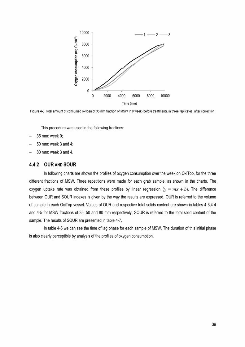
39
Figure 4-3 Total amount of consumed oxygen of 35 mm fraction of MSW in 0 week (before treatment), in three replicates, after correction.
This procedure was used in the following fractions:
35 mm: week 0;
50 mm: week 3 and 4;
80 mm: week 3 and 4.
4.4.2 OUR AND SOUR
In following charts are shown the profiles of oxygen consumption over the week on OxiTop, for the three
different fractions of MSW. Three repetitions were made for each grab sample, as shown in the charts. The
oxygen uptake rate was obtained from these profiles by linear regression (𝑦 = 𝑚𝑥 + 𝑏). The difference
between OUR and SOUR indexes is given by the way the results are expressed. OUR is referred to the volume
of sample in each OxiTop vessel. Values of OUR and respective total solids content are shown in tables 4-3,4-4
and 4-5 for MSW fractions of 35, 50 and 80 mm respectively. SOUR is referred to the total solid content of the
sample. The results of SOUR are presented in table 4-7.
In table 4-6 we can see the time of lag phase for each sample of MSW. The duration of this initial phase
is also clearly perceptible by analysis of the profiles of oxygen consumption.
0
2000
4000
6000
8000
10000
0 2000 4000 6000 8000 10000
Oxy
gen
co
nsu
mp
tio
n (
mg
O2.
dm-3
)
Time (min)
1 2 3

40
Figure 4-4 OxiTop oxygen consumption over the week , of MSW as received, at 20ºC1: a) three repetitions of the grab sample of 35 mm;
b) three repetitions of the grab sample of 50 mm; c) two repetitions of the grab sample of 80 mm.
0
2000
4000
6000
8000
10000
0 1 2 3 4 5 6 7
Oxy
gen
co
nsu
mp
tio
n (
mg
O2/
dm-3
)
Time (days)
1 2 3
0
1000
2000
3000
4000
5000
6000
0 1 2 3 4 5 6 7
Oxy
gen
co
nsu
mp
tio
n (m
g O
2.dm
-3)
Time (days)
0
1000
2000
3000
4000
5000
6000
0 1 2 3 4 5 6 7
Oxy
gen
co
nsu
mp
tio
n (m
g O
2.dm
-3)
Time (days)
a)
b)
c)
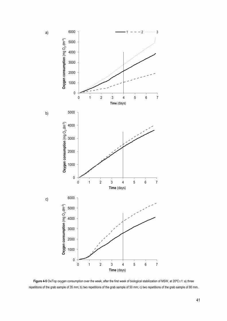
41
Figure 4-5 OxiTop oxygen consumption over the week, after the first week of biological stabilization of MSW, at 20ºC1: a) three
repetitions of the grab sample of 35 mm; b) two repetitions of the grab sample of 50 mm; c) two repetitions of the grab sample of 80 mm.
0
1000
2000
3000
4000
5000
6000
0 1 2 3 4 5 6 7
Oxy
gen
co
nsu
mp
tio
n (
mg
O2.
dm-3
)
Time (days)
1 2 3
0
1000
2000
3000
4000
5000
0 1 2 3 4 5 6 7
Oxy
gen
co
nsu
mp
tio
n (
mg
O2.
dm-3
)
Time (days)
0
1000
2000
3000
4000
5000
6000
0 1 2 3 4 5 6 7
Oxy
gen
co
nsu
mp
tio
n (
mg
O2.
dm-3
)
Time (days)
a)
b)
c)
42
Figure 4-6 OxiTop oxygen consumption over the week, after the second week of biological stabilization of MSW, at 20ºC1: a) two
repetitions of the grab sample of 35 mm; b) three repetitions of the grab sample of 50 mm; c) two repetitions of the grab sample of 80 mm.
0
1000
2000
3000
4000
5000
0 1 2 3 4 5 6 7
Oxy
gen
co
nsu
mp
tio
n (
mg
O2.
dm-3
)
Time (days)
0
1000
2000
3000
4000
5000
6000
0 1 2 3 4 5 6 7
Oxy
gen
co
nsu
mp
tio
n (
mg
O2.
dm-3
)
Time (days)
0
1000
2000
3000
4000
5000
6000
0 1 2 3 4 5 6 7
Oxy
gen
co
nsu
mp
tio
n (
mg
O2.
dm-3
)
Time (days)
a)
b)
c)
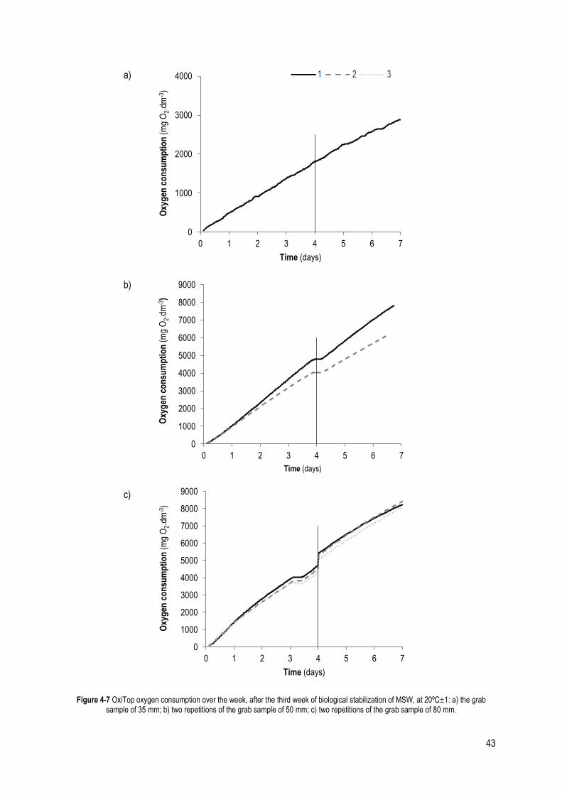
43
Figure 4-7 OxiTop oxygen consumption over the week, after the third week of biological stabilization of MSW, at 20ºC1: a) the grab sample of 35 mm; b) two repetitions of the grab sample of 50 mm; c) two repetitions of the grab sample of 80 mm.
0
1000
2000
3000
4000
0 1 2 3 4 5 6 7
Oxy
gen
co
nsu
mp
tio
n (
mg
O2.
dm-3
)
Time (days)
0
1000
2000
3000
4000
5000
6000
7000
8000
9000
0 1 2 3 4 5 6 7
Oxy
gen
co
nsu
mp
tio
n (
mg
O2.
dm-3
)
Time (days)
0
1000
2000
3000
4000
5000
6000
7000
8000
9000
0 1 2 3 4 5 6 7
Oxy
gen
co
nsu
mp
tio
n (
mg
O2.
dm-3
)
Time (days)
a)
b)
c)

44
Figure 4-8 OxiTop oxygen consumption over the week, after the fourth week of biological stabilization of MSW, at 20ºC1: a) two repetitions of the grab sample of 35 mm; b) three repetitions of the grab sample of 50 mm; c) two repetitions of the grab sample of 80 mm.
0
1000
2000
3000
4000
5000
0 1 2 3 4 5 6 7
Oxy
gen
co
nsu
mp
tio
n (
mg
O2.
dm-3
)
Time (days)
0
1000
2000
3000
4000
5000
6000
7000
0 1 2 3 4 5 6 7
Oxy
gen
co
nsu
mp
tio
n (
mg
O2.
dm-3
)
Time (days)
0
1000
2000
3000
4000
5000
6000
0 1 2 3 4 5 6 7
Oxy
gen
co
nsu
mp
tio
n (
mg
O2.
dm-3
)
Time (days)
a)
b)
c)
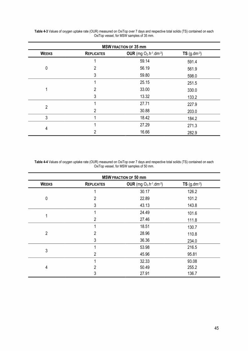
45
Table 4-3 Values of oxygen uptake rate (OUR) measured on OxiTop over 7 days and respective total solids (TS) contained on each OxiTop vessel, for MSW samples of 35 mm.
MSW FRACTION OF 35 mm
WEEKS REPLICATES OUR (mg O2.h-1.dm-3) TS (g.dm-3)
0
1 59.14 591.4
2 56.19 561.9
3 59.80 598.0
1
1 25.15 251.5
2 33.00 330.0
3 13.32 133.2
2 1 27.71 227.9
2 30.88 203.0
3 1 18.42 184.2
4 1 27.29 271.3
2 16.66 282.9
Table 4-4 Values of oxygen uptake rate (OUR) measured on OxiTop over 7 days and respective total solids (TS) contained on each OxiTop vessel, for MSW samples of 50 mm.
MSW FRACTION OF 50 mm
WEEKS REPLICATES OUR (mg O2.h-1.dm-3) TS (g.dm-3)
0
1 30.17 126.2
2 22.89 101.2
3 43.13 143.8
1 1 24.49 101.6
2 27.46 111.8
2
1 18.51 130.7
2 28.96 110.8
3 36.36 234.0
3 1 53.98 216.5
2 45.96 95.81
4
1 32.33 93.08
2 50.49 255.2
3 27.91 136.7
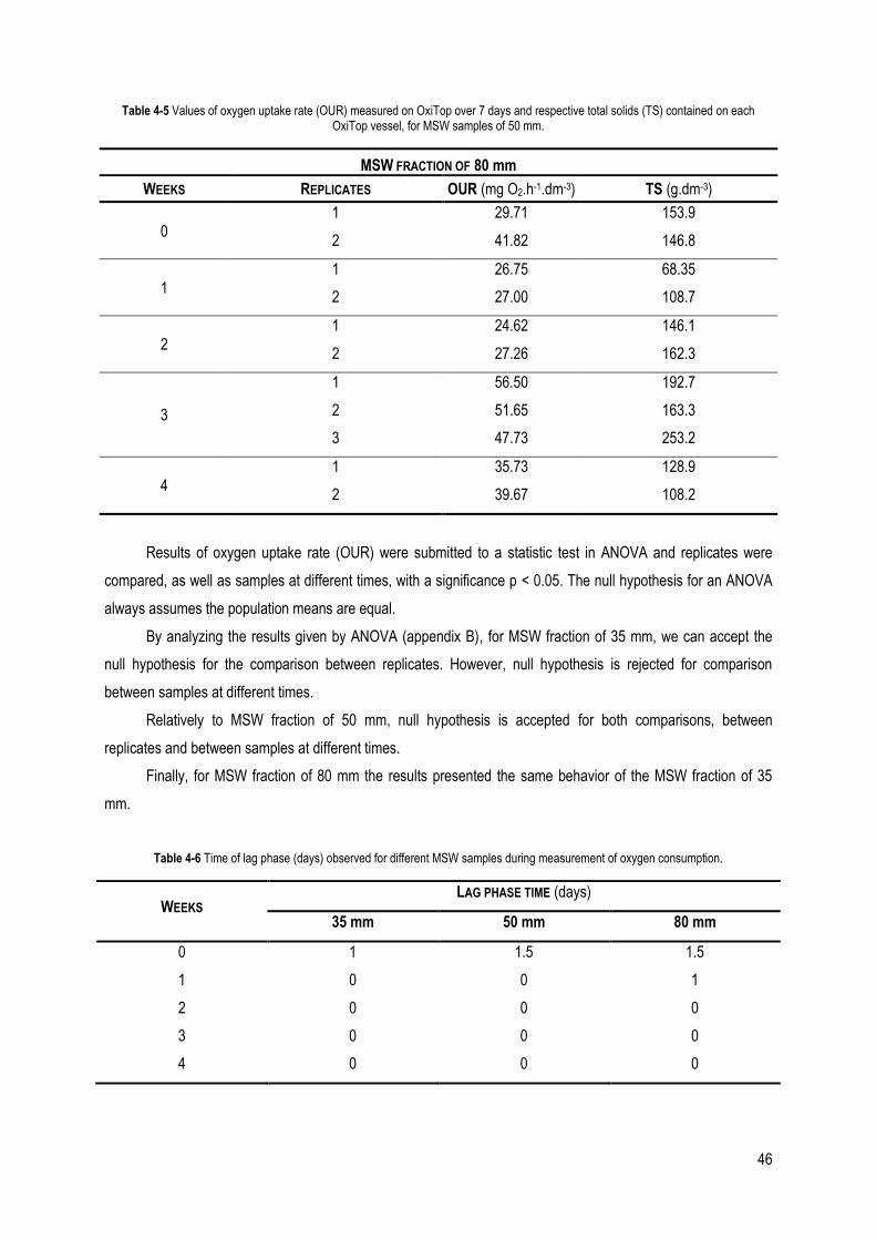
46
Table 4-5 Values of oxygen uptake rate (OUR) measured on OxiTop over 7 days and respective total solids (TS) contained on each OxiTop vessel, for MSW samples of 50 mm.
MSW FRACTION OF 80 mm
WEEKS REPLICATES OUR (mg O2.h-1.dm-3) TS (g.dm-3)
0 1 29.71 153.9
2 41.82 146.8
1 1 26.75 68.35
2 27.00 108.7
2 1 24.62 146.1
2 27.26 162.3
3
1 56.50 192.7
2 51.65 163.3
3 47.73 253.2
4 1 35.73 128.9
2 39.67 108.2
Results of oxygen uptake rate (OUR) were submitted to a statistic test in ANOVA and replicates were
compared, as well as samples at different times, with a significance p < 0.05. The null hypothesis for an ANOVA
always assumes the population means are equal.
By analyzing the results given by ANOVA (appendix B), for MSW fraction of 35 mm, we can accept the
null hypothesis for the comparison between replicates. However, null hypothesis is rejected for comparison
between samples at different times.
Relatively to MSW fraction of 50 mm, null hypothesis is accepted for both comparisons, between
replicates and between samples at different times.
Finally, for MSW fraction of 80 mm the results presented the same behavior of the MSW fraction of 35
mm.
Table 4-6 Time of lag phase (days) observed for different MSW samples during measurement of oxygen consumption.
WEEKS LAG PHASE TIME (days)
35 mm 50 mm 80 mm
0 1 1.5 1.5
1 0 0 1
2 0 0 0
3 0 0 0
4 0 0 0

47
In week 0, the lag phase time of 35 mm, 50 mm and 80 mm fractions were 1, 1.5 and 1.5 days,
respectively. In week 1, a lag phase of 1 day was observed for the 35 mm and 80 mm fractions. In the remaining
tests conducted during the stabilization time no lag phase time was observed. The absence of a lag phase
indicates the rapid growth of aerobic microorganisms in highly biodegradable substrates, i.e. the oxygen
consumption quickly starts.
Table 4-7 Time of lag phase and Specific oxygen uptake rate (SOUR) for the three fractions of MSW at the end of each week of composting process, measured in Oxitop during seven days. The results are average ± stdev (N=3).
FRACTION (mm)
WEEKS SPECIFIC OXYGEN UPTAKE RATE (SOUR)
(mg O2.g-1 TS.h-1)
35
0 0.3470.02
1 0.1970.13
2 0.1370.02*
3 0.1010.00**
4 0.0800.03*
50
0 0.2550.04
1 0.2430.00*
2 0.1860.06
3 0.3640.16*
4 0.2500.08
80
0 0.2390.06*
1 0.3200.10*
2 0.1680.00*
3 0.2660.07
4 0.3220.06*
* The results are average ± stdev (N=2);
**The result is from a single sample (without repetitions).
The specific oxygen uptake rate (SOUR) is a simple static test used to assess compost stability (Lasardi &
Stentiford, 1998). A higher degree of biological stability means a lower content of degradable organic fractions
and consequently a lower SOUR.
As shown in table 4-7, specific oxygen uptake rate of 35 mm fraction decreases significantly along the
biological stabilization process. At the end of 28 days of aerobic digestion, the compost material was more stable,
presenting a lower SOUR, as was expected.
Relatively to the MSW fractions of 50 and 80 mm, the results obtained were inconclusive. It was not visible
a decrease of SOUR as expected.
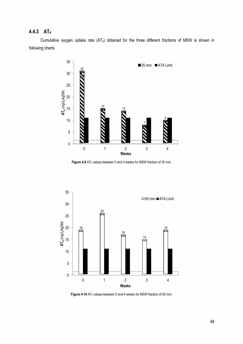
48
4.4.3 AT4
Cumulative oxygen uptake rate (AT4) obtained for the three different fractions of MSW is shown in
following charts.
Figure 4-9 AT4 values between 0 and 4 weeks for MSW fraction of 35 mm.
Figure 4-10 AT4 values between 0 and 4 weeks for MSW fraction of 50 mm.
0
5
10
15
20
25
30
35
0 1 2 3 4
30
14 13
7
9
AT
4 (m
gO2/
kgD
M)
Weeks
35 mm AT4 Limit
0
5
10
15
20
25
30
35
0 1 2 3 4
18
25
16
14
18
AT
4 (m
gO2/
kgD
M)
Weeks
50 mm AT4 Limit
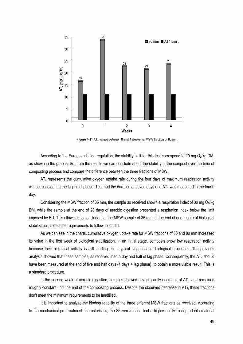
49
Figure 4-11 AT4 values between 0 and 4 weeks for MSW fraction of 80 mm.
According to the European Union regulation, the stability limit for this test correspond to 10 mg O2/kg DM,
as shown in the graphs. So, from the results we can conclude about the stability of the compost over the time of
composting process and compare the difference between the three fractions of MSW.
AT4 represents the cumulative oxygen uptake rate during the four days of maximum respiration activity
without considering the lag initial phase. Test had the duration of seven days and AT4 was measured in the fourth
day.
Considering the MSW fraction of 35 mm, the sample as received shown a respiration index of 30 mg O2/kg
DM, while the sample at the end of 28 days of aerobic digestion presented a respiration index below the limit
imposed by EU. This allows us to conclude that the MSW sample of 35 mm, at the end of one month of biological
stabilization, meets the requirements to follow to landfill.
As we can see in the charts, cumulative oxygen uptake rate for MSW fractions of 50 and 80 mm increased
its value in the first week of biological stabilization. In an initial stage, composts show low respiration activity
because their biological activity is still starting up – typical lag phase of biological processes. The previous
analysis showed that these samples, as received, had a day and half of lag phase. Consequently, the AT4 should
have been measured at the end of five and half days (4 days + lag phase), to obtain a more viable result. This is
a standard procedure.
In the second week of aerobic digestion, samples showed a significantly decrease of AT4 and remained
roughly constant until the end of the composting process. Despite the observed decrease in AT4, these fractions
don’t meet the minimum requirements to be landfilled.
It is important to analyze the biodegradability of the three different MSW fractions as received. According
to the mechanical pre-treatment characteristics, the 35 mm fraction had a higher easily biodegradable material
0
5
10
15
20
25
30
35
0 1 2 3 4
16
33
22 21
23 A
T4
(mgO
2/kg
DM
)
Weeks
80 mm AT4 Limit

50
content, while the 50 mm and 80 mm fractions had a higher biodegradable and non-biodegradable material
content. The AT4 values obtained in week 0 are in accordance with this fact, since a lower percentage of easily
biodegradable material represents a lower AT4 value.
51
5 CONCLUSIONS
The suitability of some test methods for the characterization of the biological stability of pretreated waste
before disposal in landfill and of waste deposited in landfills has been evaluated and several improvements have
been proposed (Cossu & Raga, 2008). There is no standard methodology in European Union to determine the
oxygen consumption of municipal solid waste and regulation of landfilling the treated waste materials. Member
countries of European Union have their own regulations and landfilling directives and these don’t correspond with
each other.
In this thesis the use of respirometric indices has been assessed as a reliable measure of the biological
activity of a given sample. During this study 15 respiration activity tests of samples with different sizes, as well as
from different stages of composting process were analyzed by OxiTop.
The performance of the three bio-reactors, which took place the composting process, was study, by
measurements of some parameters, such as temperature and moisture. It’s possible to conclude that there was a
correct development of the composting process.
The study carried out has demonstrated that the methodology proposed can be used for the monitoring of
stabilization of organic matter in MBT plants. The aerobic indices proved to be a good option to access biological
stability of waste because of the short duration of the assay.
The main conclusions of this study are described below:
Respiration indices are a suitable technique to measure the effect of mechanical pre-treatment on
the stabilization of municipal solid wastes that are intended to be biologically treated;
Respiration indices are a suitable technique to measure the effect of aerobic biological treatment
of municipal solid wastes that are intended to be landfilled;
Static respirometric indices, like SOUR, can be used as a first approach to characterize the solid
wastes, since it is an easy and relatively quick technique. However it cannot be considered as the
unique and reliable measure to monitor a biological process;
Cumulative respiration indices, like AT4, showed to be appropriate measure to characterize the
nature of the waste, as well as biological activity;
The quality and homogeneity of treated collected waste samples can influence highly the oxygen
consumption, leading to different AT4 values;
More parameters, such as aeration and mixing/turning, should be studied and tested during the
composting process for its corrected development.

52
Respiration indices are now considered as key parameters in the determination of the biological stability of
a compost, and hence, its quality. They are important useful tool to design the new mechanical and biological
processes according to the nature of the waste and/or to implement improvements in the facilities/processes. So,
more work needs to be done, since there are still different aspects that need more detailed investigation, both in
the mechanical and biological treatments.

53
6 REFERENCES
A
Adani, F., Lozzi, P. & Genevini, P., 2001. Determination of Biological Stability by Oxygen Uptake on
Municipal Solid Waste and Derived Products. Compost Science & Utilization, Volume 9:2, pp. 163-178.
Adani, F., Ubbiali, C. & Generini, P., 2006. The determination of biological stability of composts using the
Dynamic Respiration Index: The results of experience after two years. Waste Management, Volume 26, pp. 41-
48.
Agência Portuguesa do Ambiente, D. d. R., 2014. Relatório Anual, Resíduos Urbanos 2013, Amadora:
Agência Portuguesa do Ambiente.
B
Bakas, I., 2013. Municipal Waste Management in Portugal, Copenhagen: European Environmental
Agency.
Barrena, R. et al., 2009. In search of a reliable technique for the determination of the biological stability of
the organic matter in the mechanical-biological treated waste. Journal of Hazardous Materials, Volume 162, pp.
1065-1072.
Binner, E., Bohm, K. & Lechner, P., 2012. Large scale study on measurement of respiration activity (AT4)
by Sapromat and Oxytop. Waste Management, Volume 32, pp. 1752-1759.
Binner, E. & Zach, A., 1998. Biological Reactivity of Residual Wastes in Dependence on the Duration of
Pretreatment. Sweden: 3rd Swedish Landfill Symposium .
C
CMS, 2013. Waste Management in Central and Eastern Europe, London: Cameron McKenna’s.
Cossu, R. & Raga, R., 2008. Test methods for assessing the biological stability of biodegradable waste.,
Waste Management, Volume 28, pp. 381-388.
D
Defra, 2013. Mechanical Biological Treatment of Mechanical Biological Treatment of Municipal Solid
Waste, s.l.: Department for Environment, Food & Rural Affairs.
Di Lonardo, M., Lombardi, F. & Gavasci, R., 2012. Characterization of MBT plants input and outputs: A
review. Rev Environmental Science Biotechnology, Volume 11, p. 353–363.
Dias, N. et al., 2015. Recovery of glass from the inert fraction refused by MBT plants in a pilot plant.
Waste Management.
Dias, N., Máximo, A., Belo, N. & Carvalho, M. T., 2014. Packaging glass contained in the heavy residual
fraction refused by Portuguese Mechanical and Biological Treatment plants. Resources, Conservation and
Recycling, Volume 85, pp. 98-105.
54
Dienes, T., 2012. Environmental Assessment and Policy Options for Solid Waste Systems and
Technologies in Budapest with EASEWASTE, Budapest: Dissertation, Department of Environmental Sciences
and Policy, Central European University.
E
Epstein, E., 1997. The Science Of Composting. USA: CRC PRESS.
G
Gajalakshmi, S. & Abbasi, S., 2008. Solid Waste Management by Composting:State of the Art, Critical
Reviews in Environmental Science and Technology, Volume 38, pp. 311-400.
Gómez, R. B. et al., 2005. Respirometric assays at fixed and process temperatures to monitor composting
process. Bioresource Technology, Volume 96, p. 1153–1159.
Gómez, R. & Lima, F., 2006. The use of respiration indices in the composting process: a review. Waste
Management & Research, Volume 24, pp. 37-47.
H
Haug, R. T., 1993. The Practical Handbook of Compost Engineering. Florida: Lewis Publishers.
Herczeg, M., 2013. Municipal Waste Management in Hungary. Copenhagen: ETC/SCP.
I
Ionescu, G. et al., 2013. Integrated municipal solid waste scenario model using advanced pretreatment
and waste to energy processes. Energy Conversion and Management, Volume 76, p. 1083–1092.
K
Komilis, D. & Kanellos, D., 2012. A modified dynamic respiration test to assess compost stability: Effect of
sample size and air flowrate. Bioresource Technology, Volume 117, pp. 300-309.
Komilis, D., Kontou, I. & Ntougias, S., 2011. A modified static respiration assay and its relationship with an
enzymatic test to assess compost stability and maturity. Bioresource Technology, Volume 102, p. 5863–5872.
L
Lasardi, K. E. & Stentiford, E. I., 1998. A Simple Respirometric Technique For Assessing Compost
Stability. Water Research, Volume 32, pp. 3717-3723.
M
Magrinho, A., Didelet, F. & Semiao, V., 2006. Municipal Solid Waste Disposal in Portugal. Waste
Management, Volume 26, pp. 1477-1489.
Munnich, K., Mahler, C. & Fricke, K., 2006. Pilot project of mechanical-biological treatment of waste in
Brazil. Elsevier, Waste Management, Volume 26, p. 150–157.
Myszograj, S., Kozlowska, K. & Krochmal, A., 2014. Evaluation of biological activity of cellulose pulp by
means of the static respiration index (AT4), Poland: Civil and Environmental Engineering Reports.
55
O
Orosz, Z. & Fazekas, I., 2008. Challenges Of Municipal Waste Management in Hungary. Debrecen: AGD
Landscape & Environment 2.
S
Silva, M. & Naik, T., 2006. Overview of composting – Fundamentals and processes, USA: Center for By-
Products Utilization, University of Wisconsin-Milwaukee, Department of Civil Engineering and Mechanics.
SOER, 2015. Waste - municipal solid waste generation and management, s.l.: European Environment
Agency.
Soyes, K. & Plickert, S., 2002. Mechanical-Biological Pre-Treatment of Waste - State of the Art and
Potentials of Biotechnology, s.l.: Acta Biotechnologica.
T
Tchobanoglous, G., Theisen, H. & A. Vigil, S., 1993. Integrated Solid Waste Management, Engineering
Principles and Management issues. Singapore: McGraw-Hill International Editions.
Teixeira, S., Monteiro, E., Silva, V. & Rouboa, A., 2014. Prospective application of municipal solid wastes
for energy production in Portugal. Elsevier, 71(Energy policy), pp. 159-168.
Trautmann, N. M. & Krasny, M. E., 1997. Composting In The Classroom, USA: Cornell Waste
Management Institute.
V
Velis, C. et al., 2009. Biodrying for mechanical–biological treatment of wastes: A review of process
science and engineering. Bioresource Technology, Volume 100, p. 2747–2761.
Velis, C. et al., 2010. Production and Quality Assurance of Solid Recovered Fuels Using Mechanical—
Biological Treatment (MBT) of Waste: A Comprehensive Assessment. Critical Reviews in Environmental Science
and Technology, Volume 40, p. 979–1105.
Y
Young, C.-C., Rekha, P. & Arun, A., 2005. What happens during composting. Asian and Pacific Region:
Food&Fertilizer Technology Center Publication.

56
APPENDICES
A – Results of linear regression (OUR)
B - Statistical analysis - ANOVA
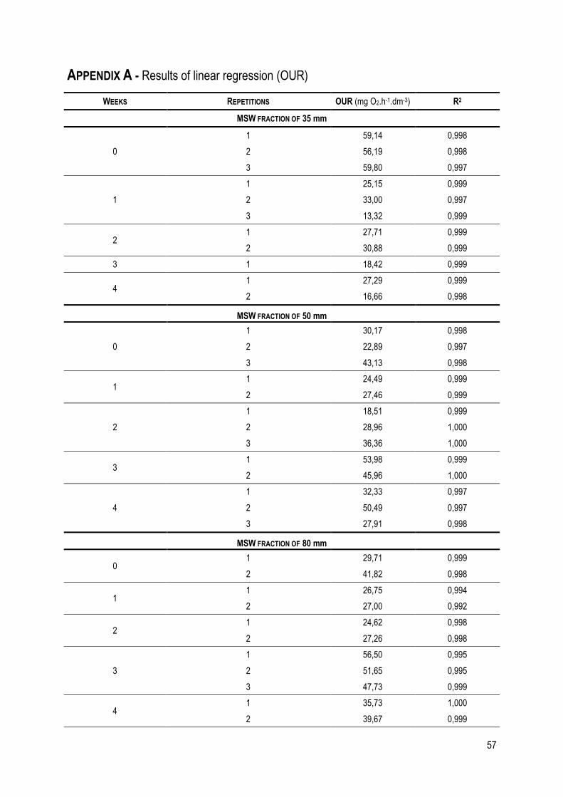
57
APPENDIX A - Results of linear regression (OUR)
WEEKS REPETITIONS OUR (mg O2.h-1.dm-3) R2
MSW FRACTION OF 35 mm
0
1 59,14 0,998
2 56,19 0,998
3 59,80 0,997
1
1 25,15 0,999
2 33,00 0,997
3 13,32 0,999
2 1 27,71 0,999
2 30,88 0,999
3 1 18,42 0,999
4 1 27,29 0,999
2 16,66 0,998
MSW FRACTION OF 50 mm
0
1 30,17 0,998
2 22,89 0,997
3 43,13 0,998
1 1 24,49 0,999
2 27,46 0,999
2
1 18,51 0,999
2 28,96 1,000
3 36,36 1,000
3 1 53,98 0,999
2 45,96 1,000
4
1 32,33 0,997
2 50,49 0,997
3 27,91 0,998
MSW FRACTION OF 80 mm
0 1 29,71 0,999
2 41,82 0,998
1 1 26,75 0,994
2 27,00 0,992
2 1 24,62 0,998
2 27,26 0,998
3
1 56,50 0,995
2 51,65 0,995
3 47,73 0,999
4 1 35,73 1,000
2 39,67 0,999

58
APPENDIX B - Statistical analysis - ANOVA
MSW FRACTION OF 35 MM
a) Comparison between repetitions
ANOVA: Single Factor
DESCRIPTION
Alpha 0,05
Groups Count Sum Mean Variance SS Std Err Lower Upper
Group 1 5 157,7046 31,54092 251,9262 1007,705 8,501883 7,935905 55,14593
Group 2 4 136,7296 34,1824 267,8645 803,5935 9,505394 3,931989 64,4328
Group 3 2 73,12458 36,56229 1079,982 1079,982 13,44266 -134,243 207,3674
ANOVA
Sources SS df MS F P value F crit RMSSE Omega
Sq
Between Groups 39,72741 2 19,86371 0,054962 0,946876 4,45897 0,132126 -0,20747
Within Groups 2891,281 8 361,4101 Total 2931,008 10 293,1008
b) Comparison between samples at different times
ANOVA: Single Factor
DESCRIPTION
Alpha 0,05
Groups Count Sum Mean Variance SS Std Err Lower Upper
Group 1 3 175,1292 58,37639 3,701777 7,403553 3,837855 41,86343 74,88935
Group 2 3 71,47417 23,82472 98,11331 196,2266 3,837855 7,311766 40,33768
Group 3 2 58,59458 29,29729 5,017848 5,017848 4,700393 -30,4269 89,02145
Group 4 1 18,41542 18,41542 #DIV/0! 0 6,647359 #NÚM! #NÚM!
Group 5 2 43,94542 21,97271 56,47631 56,47631 4,700393 -37,7514 81,69686
ANOVA
Sources SS df MS F P value F crit RMSSE Omega
Sq
Between Groups 2665,884 4 666,4709 15,08283 0,00276 4,533677 2,427772 0,836629
Within Groups 265,1243 6 44,18739 Total 2931,008 10 293,1008

59
MSW FRACTION OF 50 MM
a) Comparison between repetitions
ANOVA: Single Factor
DESCRIPTION
Alpha 0,05
Groups Count Sum Mean Variance SS Std Err Lower Upper
Group 1 5 159,4688 31,89375 181,1963 724,7853 5,368354 16,98881 46,79869
Group 2 5 175,7675 35,1535 149,9853 599,9412 5,368354 20,24856 50,05844
Group 3 3 107,4008 35,80028 58,11748 116,235 6,930516 5,980675 65,61988
ANOVA
Sources SS df MS F P value F crit RMSSE Omega
Sq
Between Groups 38,526036 2 19,26302 0,133682 0,876406 4,102821 0,174429 -0,15377
Within Groups 1440,9615 10 144,0961 Total 1479,4875 12 123,2906
b) Comparison between samples at different times
ANOVA: Single Factor
DESCRIPTION
Alpha 0,05
Groups Count Sum Mean Variance SS Std Err Lower Upper
Group 1 3 96,19541667 32,06514 105,0576 210,1152 5,37724 8,928741 55,20154
Group 2 2 51,95208333 25,97604 4,431513 4,431513 6,585747 -57,7038 109,6559
Group 3 3 83,82125 27,94042 80,44317 160,8863 5,37724 4,804019 51,07681
Group 4 2 99,9375 49,96875 32,10008 32,10008 6,585747 -33,7111 133,6486
Group 5 3 110,7308333 36,91028 143,21 286,4199 5,37724 13,77388 60,04668
ANOVA
Sources SS df MS F P value F crit RMSSE Omega
Sq
Between Groups 785,5344 4 196,3836 2,263941 0,151202 3,837853 1,028001 0,280008
Within Groups 693,9531 8 86,74414 Total 1479,488 12 123,2906
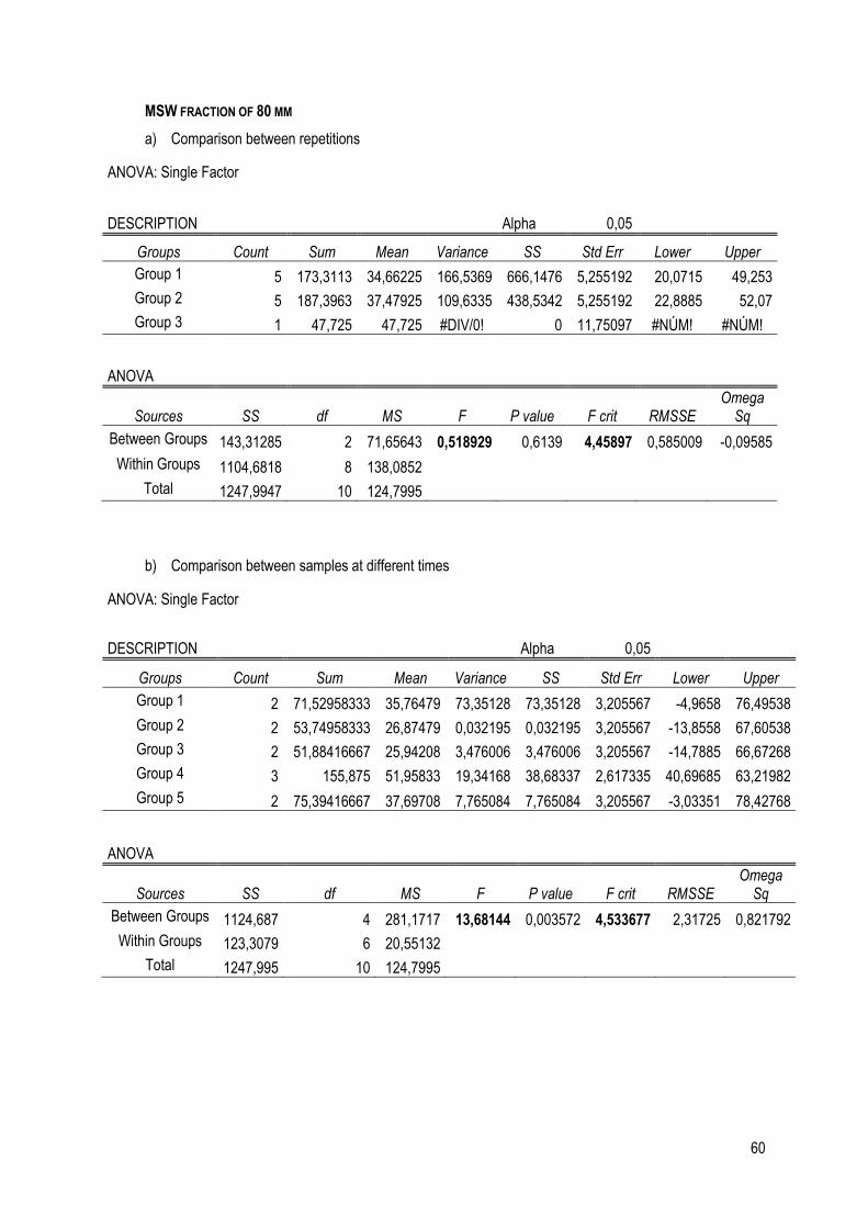
60
MSW FRACTION OF 80 MM
a) Comparison between repetitions
ANOVA: Single Factor
DESCRIPTION
Alpha 0,05
Groups Count Sum Mean Variance SS Std Err Lower Upper
Group 1 5 173,3113 34,66225 166,5369 666,1476 5,255192 20,0715 49,253
Group 2 5 187,3963 37,47925 109,6335 438,5342 5,255192 22,8885 52,07
Group 3 1 47,725 47,725 #DIV/0! 0 11,75097 #NÚM! #NÚM!
ANOVA
Sources SS df MS F P value F crit RMSSE Omega
Sq
Between Groups 143,31285 2 71,65643 0,518929 0,6139 4,45897 0,585009 -0,09585
Within Groups 1104,6818 8 138,0852 Total 1247,9947 10 124,7995
b) Comparison between samples at different times
ANOVA: Single Factor
DESCRIPTION
Alpha 0,05
Groups Count Sum Mean Variance SS Std Err Lower Upper
Group 1 2 71,52958333 35,76479 73,35128 73,35128 3,205567 -4,9658 76,49538
Group 2 2 53,74958333 26,87479 0,032195 0,032195 3,205567 -13,8558 67,60538
Group 3 2 51,88416667 25,94208 3,476006 3,476006 3,205567 -14,7885 66,67268
Group 4 3 155,875 51,95833 19,34168 38,68337 2,617335 40,69685 63,21982
Group 5 2 75,39416667 37,69708 7,765084 7,765084 3,205567 -3,03351 78,42768
ANOVA
Sources SS df MS F P value F crit RMSSE Omega
Sq
Between Groups 1124,687 4 281,1717 13,68144 0,003572 4,533677 2,31725 0,821792
Within Groups 123,3079 6 20,55132 Total 1247,995 10 124,7995
Top Related