ZEB Project report 41– 2018 Igor Sartori, Sjur V. Løtveit ... · Igor Sartori, Sjur V. Løtveit...
67
Igor Sartori, Sjur V. Løtveit and Kristian S. Skeie ZEB Project report 41– 2018 Guidelines on energy system analysis and cost optimality in early design of ZEB
Transcript of ZEB Project report 41– 2018 Igor Sartori, Sjur V. Løtveit ... · Igor Sartori, Sjur V. Løtveit...
Igor Sartori, Sjur V. Løtveit and Kristian S. Skeie
ZEB Project report 41– 2018
www.zeb.no
Guidelines on energy system analysis and cost optimality in early design of ZEB
Igor Sartori, Sjur V. Løtveit and Kristian S. Skeie
Guidelines on energy system analysis and cost optimality in early design of ZEB
ZEB Project report 41 – 2018
SINTEF Academic Press

ZEB Project report no 41Igor Sartori2), Sjur V. Løtveit1) and Kristian S. Skeie1)
Guidelines on energy system analysis and cost optimality in early design of ZEB
Keywords:ZEB energy system; techno-economic analysis; early design phase
Illustration on front page: ????
ISSN 1893-157X (online)ISSN 1893-1561ISBN 978-82-536-1577-6 (pdf)
© Copyright SINTEF Academic Press and Norwegian University of Science and Technology 2018The material in this publication is covered by the provisions of the Norwegian Copyright Act. Without any special agreement with SINTEF Academic Press and Norwegian University of Science and Technology, any copying and making available of the material is only allowed to the extent that this is permitted by law or allowed through an agreement with Kopinor, the Reproduction Rights Organisation for Norway. Any use contrary to legislation or an agreement may lead to a liability for damages and confiscation, and may be punished by fines or imprisonment.
SINTEF Building and Infrastructure Trondheim 2)
Høgskoleringen 7 b, Postbox 4760 Sluppen, N-7465 TrondheimTel: +47 73 59 30 00www.sintef.no/byggforskwww.zeb.no
Norwegian University of Science and Technology 1)
N-7491 TrondheimTel: +47 73 59 50 00www.ntnu.nowww.zeb.no
SINTEF Academic Pressc/o SINTEF Building and Infrastructure OsloForskningsveien 3 B, Postbox 124 Blindern, N-0314 OsloTel: +47 73 59 30 00, Fax: +47 22 69 94 38www.sintef.no/byggforskwww.sintefbok.no

ZEB Project report 41-2017 Page 3 of 65
Acknowledgement
These guidelines and templates are developed within ZEB-WP3 «Energy supply systems and services». This ZEB work package focuses on energy supply, building services, indoor environment and building interaction, increasingly important in buildings with better thermal envelopes and inclusion of on-site renewables. To avoid suboptimal solutions, tools are developed to find the best combination of different energy supply sources with regard to emissions and economy. This report has been written within the Research Centre on Zero Emission Buildings (ZEB). The authors gratefully acknowledge the support from the Research Council of Norway, BNL – Federation of construction industries, Brødrene Dahl, ByBo, DiBK – Norwegian Building Authority, Caverion Norge AS, DuPont, Entra, Forsvarsbygg, Glava, Husbanken, Isola, Multiconsult, NorDan, Norsk Teknologi, Protan, SAPA Building Systems, Skanska, Snøhetta, Statsbygg, Sør-Trøndelag Fylkeskommune, and Weber. We would also like to thank all the practitioners who has given valuable feedback on the tool during the testing phase. Thanks to Andreas Kissavosin EQUA AB for development of the output script for IDA-ICE.
ZEB Project report 41-2017 Page 4 of 65
Abstract
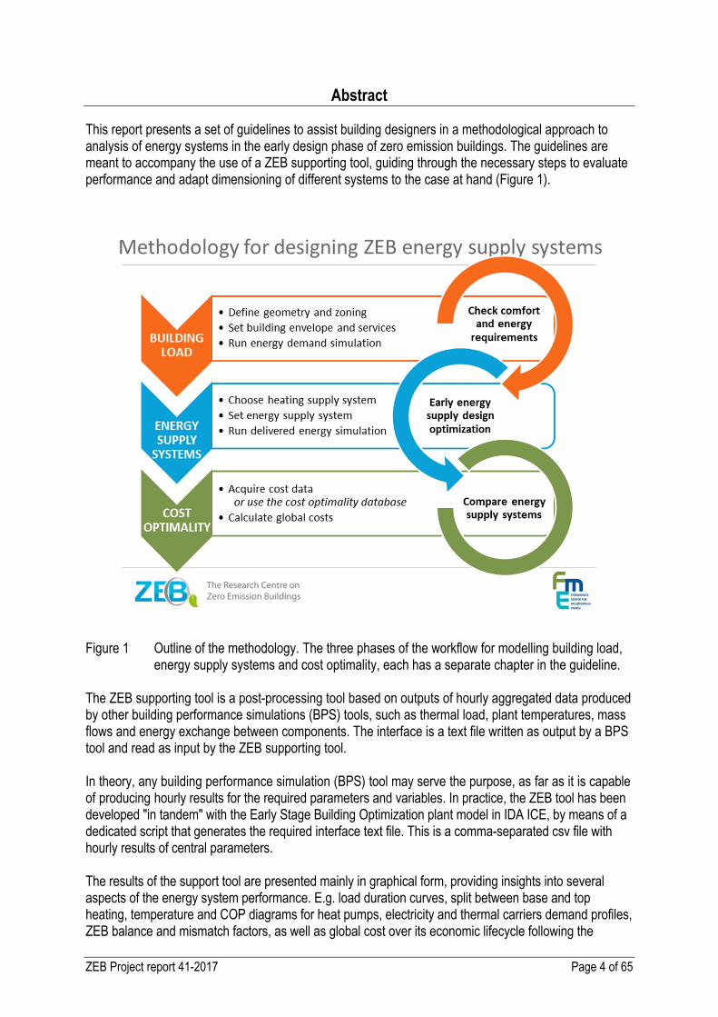
This report presents a set of guidelines to assist building designers in a methodological approach to analysis of energy systems in the early design phase of zero emission buildings. The guidelines are meant to accompany the use of a ZEB supporting tool, guiding through the necessary steps to evaluate performance and adapt dimensioning of different systems to the case at hand (Figure 1).
Figure 1 Outline of the methodology. The three phases of the workflow for modelling building load,
energy supply systems and cost optimality, each has a separate chapter in the guideline. The ZEB supporting tool is a post-processing tool based on outputs of hourly aggregated data produced by other building performance simulations (BPS) tools, such as thermal load, plant temperatures, mass flows and energy exchange between components. The interface is a text file written as output by a BPS tool and read as input by the ZEB supporting tool. In theory, any building performance simulation (BPS) tool may serve the purpose, as far as it is capable of producing hourly results for the required parameters and variables. In practice, the ZEB tool has been developed "in tandem" with the Early Stage Building Optimization plant model in IDA ICE, by means of a dedicated script that generates the required interface text file. This is a comma-separated csv file with hourly results of central parameters. The results of the support tool are presented mainly in graphical form, providing insights into several aspects of the energy system performance. E.g. load duration curves, split between base and top heating, temperature and COP diagrams for heat pumps, electricity and thermal carriers demand profiles, ZEB balance and mismatch factors, as well as global cost over its economic lifecycle following the

ZEB Project report 41-2017 Page 5 of 65
principles of cost optimality (Cost-optimal methodology and accompanying technical guidelines, EU 244/2012). Chapter 6 discusses the feedback from a test carried out by Norwegian BPS practitioners and the possibility for further research and development of the tool. For the time being the ZEB tool is implemented as an Excel spreadsheet with embedded VBA (Visual Basic) code, thus favouring transparency and easiness of use over flexibility and computational performance. When standards and methods are in place, the tool can be further developed in other environments, e.g. Matlab, and/or directly incorporated into existing BPS tools.

ZEB Project report 41-2017 Page 6 of 65
Nomenclature
Table of abbreviations
AHU - Air Handling Unit
AWHP - Air to Water Heat Pump
BPS - Building Performance Simulations
CHP boiler - Combined Heat and Power boiler
DHW - Domestic Hot Water
EPBD - Energy Performance of Buildings Directive
ESBO plant - Early Stage Building Optimisation plant
GSHP - Ground Source Heat Pump
HVAC - Heating Ventilating and Air Conditioning
IDA-ICE - IDA Indoor Climate and Energy by EQUA simulation AB [www.equa.se]
PI-controller - Proportional-Integral controller [Wikipedia]
PV-panels - Photo voltaic panels
ST-collectors - Solar thermal collectors
ZEB - Zero Emission Building
ZEB Project report 41-2017 Page 7 of 65
Contents
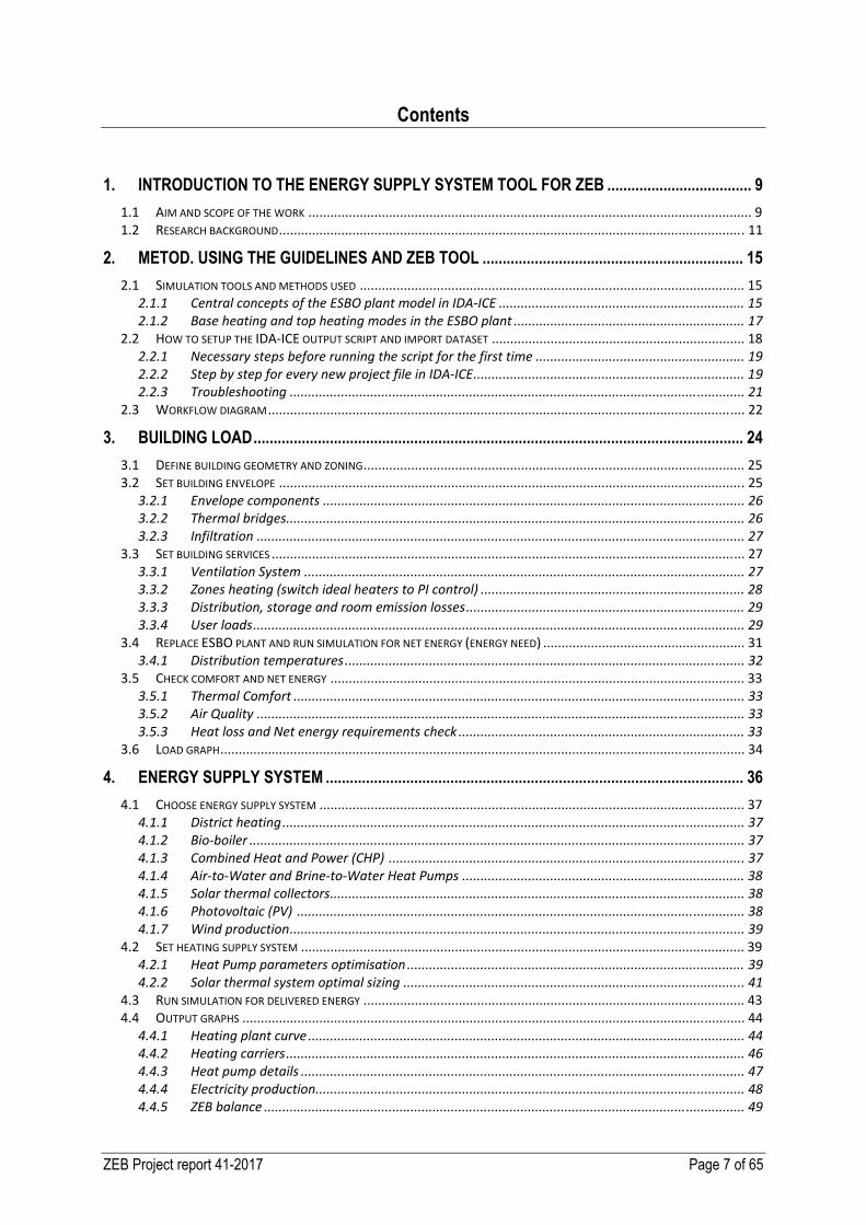
1. INTRODUCTION TO THE ENERGY SUPPLY SYSTEM TOOL FOR ZEB .................................... 9
1.1 AIM AND SCOPE OF THE WORK ......................................................................................................................... 9 1.2 RESEARCH BACKGROUND ............................................................................................................................... 11
2. METOD. USING THE GUIDELINES AND ZEB TOOL ................................................................. 15
2.1 SIMULATION TOOLS AND METHODS USED ......................................................................................................... 15 2.1.1 Central concepts of the ESBO plant model in IDA-ICE ................................................................... 15 2.1.2 Base heating and top heating modes in the ESBO plant ............................................................... 17
2.2 HOW TO SETUP THE IDA-ICE OUTPUT SCRIPT AND IMPORT DATASET ..................................................................... 18 2.2.1 Necessary steps before running the script for the first time ......................................................... 19 2.2.2 Step by step for every new project file in IDA-ICE .......................................................................... 19 2.2.3 Troubleshooting ............................................................................................................................ 21
2.3 WORKFLOW DIAGRAM .................................................................................................................................. 22
3. BUILDING LOAD .......................................................................................................................... 24
3.1 DEFINE BUILDING GEOMETRY AND ZONING ........................................................................................................ 25 3.2 SET BUILDING ENVELOPE ............................................................................................................................... 25
3.2.1 Envelope components ................................................................................................................... 26 3.2.2 Thermal bridges............................................................................................................................. 26 3.2.3 Infiltration ..................................................................................................................................... 27
3.3 SET BUILDING SERVICES ................................................................................................................................. 27 3.3.1 Ventilation System ........................................................................................................................ 27 3.3.2 Zones heating (switch ideal heaters to PI control) ........................................................................ 28 3.3.3 Distribution, storage and room emission losses ............................................................................ 29 3.3.4 User loads ...................................................................................................................................... 29
3.4 REPLACE ESBO PLANT AND RUN SIMULATION FOR NET ENERGY (ENERGY NEED) ....................................................... 31 3.4.1 Distribution temperatures ............................................................................................................. 32
3.5 CHECK COMFORT AND NET ENERGY ................................................................................................................. 33 3.5.1 Thermal Comfort ........................................................................................................................... 33 3.5.2 Air Quality ..................................................................................................................................... 33 3.5.3 Heat loss and Net energy requirements check .............................................................................. 33
3.6 LOAD GRAPH ............................................................................................................................................... 34
4. ENERGY SUPPLY SYSTEM ........................................................................................................ 36
4.1 CHOOSE ENERGY SUPPLY SYSTEM .................................................................................................................... 37 4.1.1 District heating .............................................................................................................................. 37 4.1.2 Bio-boiler ....................................................................................................................................... 37 4.1.3 Combined Heat and Power (CHP) ................................................................................................. 37 4.1.4 Air-to-Water and Brine-to-Water Heat Pumps ............................................................................. 38 4.1.5 Solar thermal collectors ................................................................................................................. 38 4.1.6 Photovoltaic (PV) .......................................................................................................................... 38 4.1.7 Wind production ............................................................................................................................ 39
4.2 SET HEATING SUPPLY SYSTEM ......................................................................................................................... 39 4.2.1 Heat Pump parameters optimisation ............................................................................................ 39 4.2.2 Solar thermal system optimal sizing ............................................................................................. 41
4.3 RUN SIMULATION FOR DELIVERED ENERGY ........................................................................................................ 43 4.4 OUTPUT GRAPHS ......................................................................................................................................... 44
4.4.1 Heating plant curve ....................................................................................................................... 44 4.4.2 Heating carriers ............................................................................................................................. 46 4.4.3 Heat pump details ......................................................................................................................... 47 4.4.4 Electricity production ..................................................................................................................... 48 4.4.5 ZEB balance ................................................................................................................................... 49

ZEB Project report 41-2017 Page 8 of 65
5. COST OPTIMALITY ...................................................................................................................... 50
5.1 CALCULATION OF GLOBAL COSTS ..................................................................................................................... 50 5.1.1 Product Database .......................................................................................................................... 50 5.1.2 Cost analysis tool ........................................................................................................................... 50
5.2 COMPARE DIFFERENT ENERGY SUPPLY SYSTEMS .................................................................................................. 52
6. DISCUSSION AND CONCLUSIONS ............................................................................................ 54
6.1 DISCUSSION ................................................................................................................................................ 54 6.2 CONCLUSION .............................................................................................................................................. 56
7. REFERENCES .............................................................................................................................. 57
APPENDICES

ZEB Project report 41-2017 Page 9 of 65
1. Introduction to the energy supply system tool for ZEB
1.1 Aim and scope of the work
This report presents a set of guidelines to assist building designers in a methodological approach to analysis of energy systems in the early design phase of zero emission buildings (ZEB). The guidelines are meant to accompany the use of a ZEB supporting tool, guiding through the necessary steps to evaluate performance and adapt dimensioning of different systems to the case at hand (Figure 1). The guidelines show an example of a residential apartment building model where different energy supply systems are compared to ZEB performance metrics.
The Excel supporting tools are developed for a specific BPS software suite, but in principle, the same methodology could be used for other software, and the templates could be adapted to import other data formats than results from IDA-ICE.
The basis for the cost database is collected through a master thesis work (Løtveit, 2013).
Figure 2 Outline of the methodology. The three phases of the workflow for modelling building load,
energy supply systems and cost optimality, each has a separate chapter in the guideline.
This report is built around a method for designing ZEB energy supply system described in Figure 2. Before being guided through the method for designing ZEB energy supply systems, the reader will be introduced to the concept of Zero Emission Buildings and the Norwegian ZEB centre's ambition levels in Chapter 1, where the basic concept of balancing a building’s operational energy and emissions with on-site production will be explained. In theory, any building performance simulation (BPS) tool may serve the purpose, as far as it is capable of producing hourly results for the required parameters and variables.
ZEB Project report 41-2017 Page 10 of 65
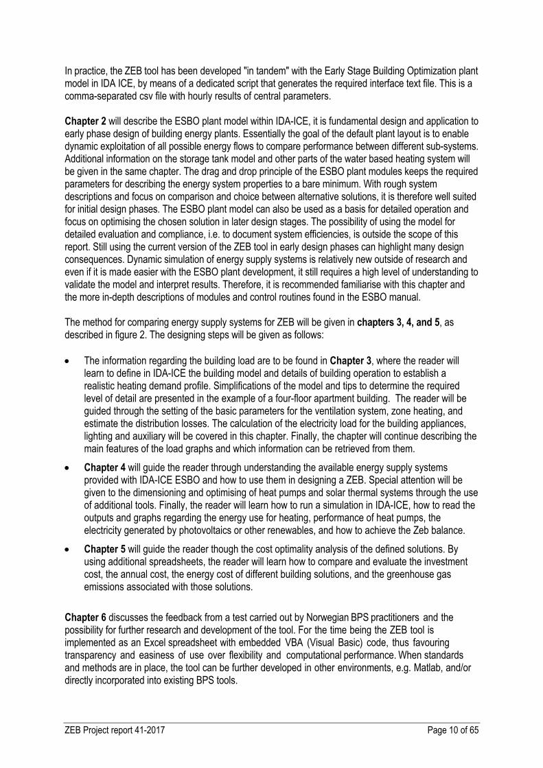
In practice, the ZEB tool has been developed "in tandem" with the Early Stage Building Optimization plant model in IDA ICE, by means of a dedicated script that generates the required interface text file. This is a comma-separated csv file with hourly results of central parameters. Chapter 2 will describe the ESBO plant model within IDA-ICE, it is fundamental design and application to early phase design of building energy plants. Essentially the goal of the default plant layout is to enable dynamic exploitation of all possible energy flows to compare performance between different sub-systems. Additional information on the storage tank model and other parts of the water based heating system will be given in the same chapter. The drag and drop principle of the ESBO plant modules keeps the required parameters for describing the energy system properties to a bare minimum. With rough system descriptions and focus on comparison and choice between alternative solutions, it is therefore well suited for initial design phases. The ESBO plant model can also be used as a basis for detailed operation and focus on optimising the chosen solution in later design stages. The possibility of using the model for detailed evaluation and compliance, i.e. to document system efficiencies, is outside the scope of this report. Still using the current version of the ZEB tool in early design phases can highlight many design consequences. Dynamic simulation of energy supply systems is relatively new outside of research and even if it is made easier with the ESBO plant development, it still requires a high level of understanding to validate the model and interpret results. Therefore, it is recommended familiarise with this chapter and the more in-depth descriptions of modules and control routines found in the ESBO manual. The method for comparing energy supply systems for ZEB will be given in chapters 3, 4, and 5, as described in figure 2. The designing steps will be given as follows: The information regarding the building load are to be found in Chapter 3, where the reader will
learn to define in IDA-ICE the building model and details of building operation to establish a realistic heating demand profile. Simplifications of the model and tips to determine the required level of detail are presented in the example of a four-floor apartment building. The reader will be guided through the setting of the basic parameters for the ventilation system, zone heating, and estimate the distribution losses. The calculation of the electricity load for the building appliances, lighting and auxiliary will be covered in this chapter. Finally, the chapter will continue describing the main features of the load graphs and which information can be retrieved from them.
Chapter 4 will guide the reader through understanding the available energy supply systems provided with IDA-ICE ESBO and how to use them in designing a ZEB. Special attention will be given to the dimensioning and optimising of heat pumps and solar thermal systems through the use of additional tools. Finally, the reader will learn how to run a simulation in IDA-ICE, how to read the outputs and graphs regarding the energy use for heating, performance of heat pumps, the electricity generated by photovoltaics or other renewables, and how to achieve the Zeb balance.
Chapter 5 will guide the reader though the cost optimality analysis of the defined solutions. By using additional spreadsheets, the reader will learn how to compare and evaluate the investment cost, the annual cost, the energy cost of different building solutions, and the greenhouse gas emissions associated with those solutions.
Chapter 6 discusses the feedback from a test carried out by Norwegian BPS practitioners and the possibility for further research and development of the tool. For the time being the ZEB tool is implemented as an Excel spreadsheet with embedded VBA (Visual Basic) code, thus favouring transparency and easiness of use over flexibility and computational performance. When standards and methods are in place, the tool can be further developed in other environments, e.g. Matlab, and/or directly incorporated into existing BPS tools.

ZEB Project report 41-2017 Page 11 of 65
1.2 Research background
Previous work within ZEB WP-3 amongst building designers, both architects and engineers, highlighted the need for more knowledge and better supporting tools for the choice of energy systems for ZEBs. In the IEA-SHC task 401 several studies focus on current software’s capabilities to support early design of Net zero solar energy buildings (NZEBs), a survey among practitioners of building performance simulations (BPS) and interviews with simulation experts are published (Attia et.al., 2009, 2010, 2011, 2012). Requirements for a BPS energy supply tool to support ZEB design Most of the building performance simulation (BPS) tools available today address the later design stages and are consequently used for documentation and evaluation purposes. In a review of ten tools for the early design phase (Attia, 2012), it is concluded that these tools need to become more effective and informative in order to support design decisions. Attia suggests from the feedback of a questionnaire among architects and engineers that the users are confident with those tools that are (to some extent) shared by the whole design team. It is clear that in order to integrate BPS in the design process, tools must communicate to different users (architects, engineers, experts etc.), by using familiar language. If tools are meant to cater for different stakeholders (also possibly owners, and facility managers), data needs to be represented in a clear and honest way. Transparency is a central aspect, as well as the reduction process that occurs when results from simulation are post-processed, reported, and presented to the design team. In a recent study (Loukisas 2013) among building designers, it is found that today both architects and engineers are using simulations to negotiate a relationship. Loukissas claims that new forms of creativity and control emerge. Building performance simulations have a high value in answering why, when, and how buildings behave energy-wise, and do not need to be mere presentations of aggregated data (e.g., total annual energy consumption) of the predicted building performance. Insightful presentations of results allow multiple scenarios and “what if” questions to be answered without necessarily performing incremental one-change-at-a-time simulations (O'Brien, 2012). However, encouraging the use of BPS tools in early stage building design remains a challenge. This is partly because many BPS tools require detailed design specifications (which take significant time to collect and input) to be operated, and because the types of output do not inform designers on how to improve their design. O'Brien suggests that processes over which the designer has the greatest amount of control should be the focus of the early phase modeling effort and analysis, to be presented and discussed in detail within the design team. In designing ZEBs, it is therefore necessary to go beyond what is possible with standard compliance tools such as Simien and TEK-sjekk. To go beyond the building code requirements, it is necessary to focus both on energy efficiency and on the complete dimensioning of building and energy systems. For ZEB building design this also mean to assess other metrics such as the load-generation match, the carbon emission accounting, and the power exchange with the grid. Indeed practitioners in the Attia's survey reported that they need tools that can produce initial results from rough representations during early stage and in the same time allow for detailing of building components during later phases. In a design process there is often a lack of time and resources to verify simulations. Therefore, there is a need for tools that can help to take decisions on the basis of very limited knowledge. Furthermore, different levels of sophistication are needed depending on the complexity, innovation and risk involved in the project.
1 International Energy Agency (IEA) – Solar Heating and Cooling programme (SHC) Task 40 / Energy in Buildings and Communities Programme (EBC) Annex 52: Towards Net Zero Energy Solar Buildings, http://task40.iea-shc.org/
ZEB Project report 41-2017 Page 12 of 65
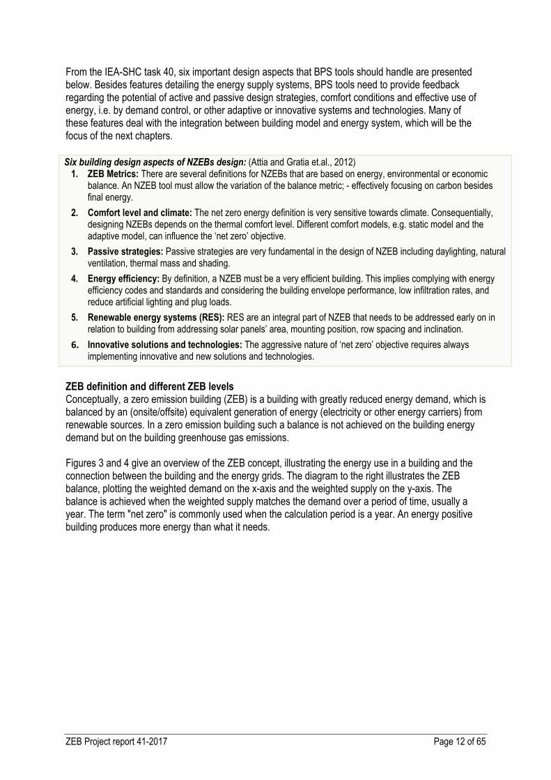
From the IEA-SHC task 40, six important design aspects that BPS tools should handle are presented below. Besides features detailing the energy supply systems, BPS tools need to provide feedback regarding the potential of active and passive design strategies, comfort conditions and effective use of energy, i.e. by demand control, or other adaptive or innovative systems and technologies. Many of these features deal with the integration between building model and energy system, which will be the focus of the next chapters. Six building design aspects of NZEBs design: (Attia and Gratia et.al., 2012)
1. ZEB Metrics: There are several definitions for NZEBs that are based on energy, environmental or economic balance. An NZEB tool must allow the variation of the balance metric; - effectively focusing on carbon besides final energy.
2. Comfort level and climate: The net zero energy definition is very sensitive towards climate. Consequentially, designing NZEBs depends on the thermal comfort level. Different comfort models, e.g. static model and the adaptive model, can influence the ‘net zero’ objective.
3. Passive strategies: Passive strategies are very fundamental in the design of NZEB including daylighting, natural ventilation, thermal mass and shading.
4. Energy efficiency: By definition, a NZEB must be a very efficient building. This implies complying with energy efficiency codes and standards and considering the building envelope performance, low infiltration rates, and reduce artificial lighting and plug loads.
5. Renewable energy systems (RES): RES are an integral part of NZEB that needs to be addressed early on in relation to building from addressing solar panels’ area, mounting position, row spacing and inclination.
6. Innovative solutions and technologies: The aggressive nature of ‘net zero’ objective requires always implementing innovative and new solutions and technologies.
ZEB definition and different ZEB levels Conceptually, a zero emission building (ZEB) is a building with greatly reduced energy demand, which is balanced by an (onsite/offsite) equivalent generation of energy (electricity or other energy carriers) from renewable sources. In a zero emission building such a balance is not achieved on the building energy demand but on the building greenhouse gas emissions. Figures 3 and 4 give an overview of the ZEB concept, illustrating the energy use in a building and the connection between the building and the energy grids. The diagram to the right illustrates the ZEB balance, plotting the weighted demand on the x-axis and the weighted supply on the y-axis. The balance is achieved when the weighted supply matches the demand over a period of time, usually a year. The term "net zero" is commonly used when the calculation period is a year. An energy positive building produces more energy than what it needs.
ZEB Project report 41-2017 Page 13 of 65
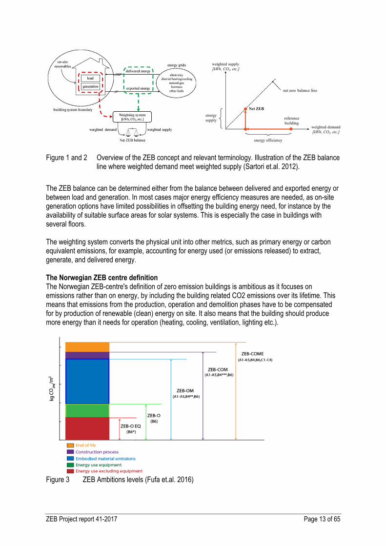
Figure 1 and 2 Overview of the ZEB concept and relevant terminology. Illustration of the ZEB balance
line where weighted demand meet weighted supply (Sartori et.al. 2012).
The ZEB balance can be determined either from the balance between delivered and exported energy or between load and generation. In most cases major energy efficiency measures are needed, as on-site generation options have limited possibilities in offsetting the building energy need, for instance by the availability of suitable surface areas for solar systems. This is especially the case in buildings with several floors. The weighting system converts the physical unit into other metrics, such as primary energy or carbon equivalent emissions, for example, accounting for energy used (or emissions released) to extract, generate, and delivered energy. The Norwegian ZEB centre definition The Norwegian ZEB-centre's definition of zero emission buildings is ambitious as it focuses on emissions rather than on energy, by including the building related CO2 emissions over its lifetime. This means that emissions from the production, operation and demolition phases have to be compensated for by production of renewable (clean) energy on site. It also means that the building should produce more energy than it needs for operation (heating, cooling, ventilation, lighting etc.).
Figure 3 ZEB Ambitions levels (Fufa et.al. 2016)
ZEB Project report 41-2017 Page 14 of 65
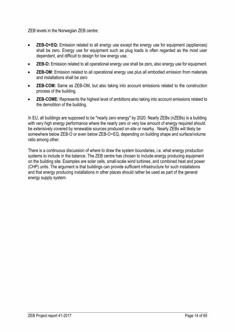
ZEB levels in the Norwegian ZEB centre:
ZEB-O÷EQ: Emission related to all energy use except the energy use for equipment (appliances) shall be zero. Energy use for equipment such as plug loads is often regarded as the most user dependent, and difficult to design for low energy use.
ZEB-O: Emission related to all operational energy use shall be zero, also energy use for equipment.
ZEB-OM: Emission related to all operational energy use plus all embodied emission from materials and installations shall be zero
ZEB-COM: Same as ZEB-OM, but also taking into account emissions related to the construction process of the building.
ZEB-COME: Represents the highest level of ambitions also taking into account emissions related to the demolition of the building.
In EU, all buildings are supposed to be "nearly zero energy" by 2020. Nearly ZEBs (nZEBs) is a building with very high energy performance where the nearly zero or very low amount of energy required should be extensively covered by renewable sources produced on-site or nearby. Nearly ZEBs will likely be somewhere below ZEB-O or even below ZEB-O÷EQ, depending on building shape and surface/volume ratio among other. There is a continuous discussion of where to draw the system boundaries, i.e. what energy production systems to include in the balance. The ZEB centre has chosen to include energy producing equipment on the building site. Examples are solar cells, small-scale wind turbines, and combined heat and power (CHP) units. The argument is that buildings can provide sufficient infrastructure for such installations and that energy producing installations in other places should rather be used as part of the general energy supply system.
ZEB Project report 41-2017 Page 15 of 65
2. Metod. Using the Guidelines and ZEB Tool
In the following section, the central concept of the ESBO plant is presented. Detailed steps to enable the ESBO plant model and run the simulation script are found in the next section (2.2). The workflow for comparing different energy supply systems is outlined in a process diagram (Figure 13) at the end of this chapter, in Section 2.3. The diagram gives an overview of where in the process Excel support tools are available. The three next chapters are dedicated to the necessary steps to define a building load, choose an energy supply system for the building model and perform a global cost calculation. The whole process can be repeated for as many systems or design variations that are needed to be compared, as indicated in the process diagram (Figure 13).
2.1 Simulation tools and methods used
Outlining the requirements for building performance tools to specifically support ZEB design in the previous section, in most construction projects it is not common practice to simulate energy supply systems. Typically, the design dimensioning and choice of components, temperature levels and layouts of systems is based on rules of thumb and basic analysis. Integrated models of the interaction between the building and the energy system are only implemented and validated in a handful of programs. For this purpose, the most used software suites are TRNSYS, EnergyPlus and IDA-ICE (Crawley, 2008). Though actively used in research for many years, recent developments are extending their usability and presenting opportunities to use these tools in new ways to take informed design decisions. Internationally, the IEA EBC Annex 602 is focused on further software development that allows buildings and community energy grids to be designed and operated as integrated, robust, and efficient systems. IDA-ICE is chosen because it is gaining momentum amongst Norwegian practitioners. The platform offers both a good balance between solid mathematical modelling and a user-friendly graphical interface. The modelling environment is equation based, providing a possibility to model physical phenomena by simply describing their governing equations3, without the need of writing the code that solves those equations. EnergyPlus is also going in this direction which is by some termed as the next generation of equation-based and object-oriented modelling (Wetter, 2012). There are four levels of the IDA-ICA modelling environment: ESBO (Early Stage Building Optimization), standard, advanced and developer interface. Most works happen at the standard level, and only in few cases it is necessary to work/run simulations at the advanced level. With these guidelines we work at the standard level with the inclusion of the ESBO plant model. 2.1.1 Central concepts of the ESBO plant model in IDA-ICE
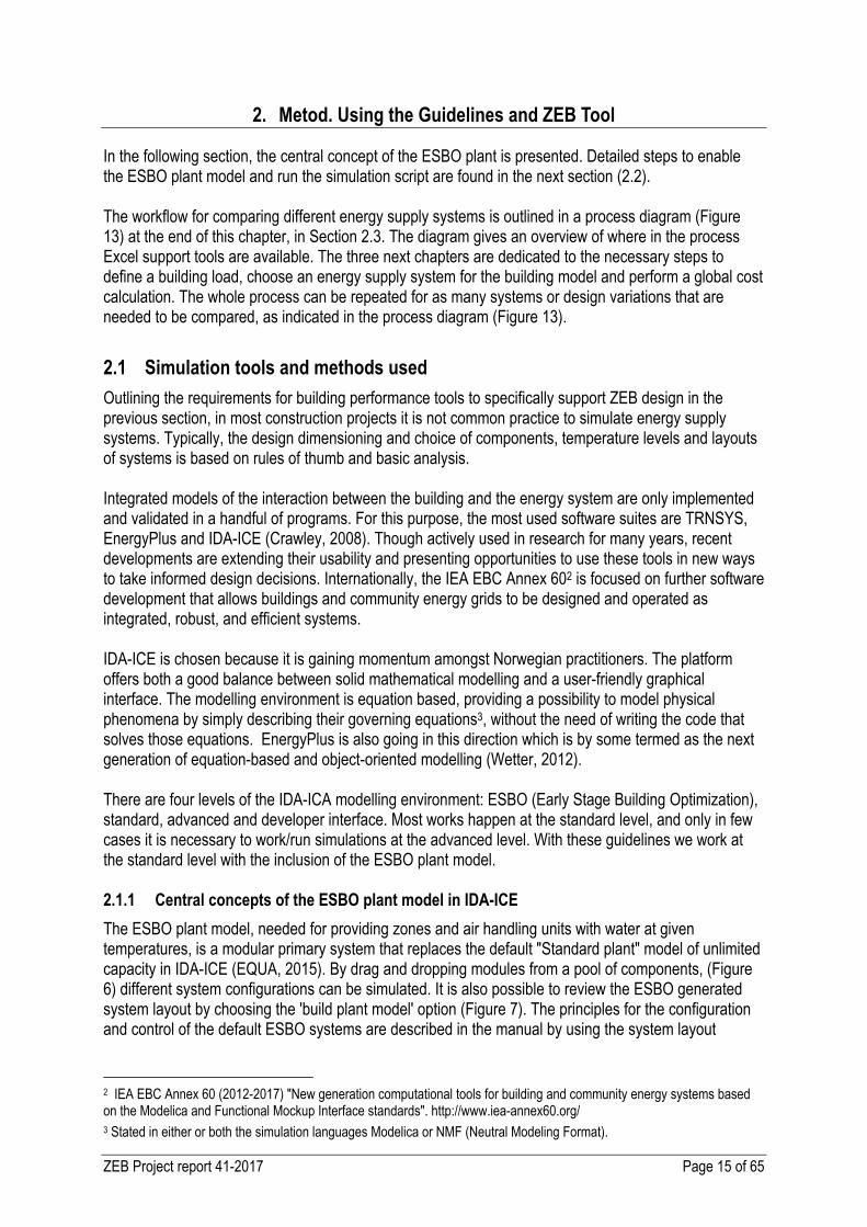
The ESBO plant model, needed for providing zones and air handling units with water at given temperatures, is a modular primary system that replaces the default "Standard plant" model of unlimited capacity in IDA-ICE (EQUA, 2015). By drag and dropping modules from a pool of components, (Figure 6) different system configurations can be simulated. It is also possible to review the ESBO generated system layout by choosing the 'build plant model' option (Figure 7). The principles for the configuration and control of the default ESBO systems are described in the manual by using the system layout
2 IEA EBC Annex 60 (2012-2017) "New generation computational tools for building and community energy systems based on the Modelica and Functional Mockup Interface standards". http://www.iea-annex60.org/ 3 Stated in either or both the simulation languages Modelica or NMF (Neutral Modeling Format).
ZEB Project report 41-2017 Page 16 of 65
(EQUA, 2015). Besides, the software code of each component provides comments and documentation about the mathematical models, which can be viewed from within the program. A decentralised control strategy The purpose of the default ESBO system configurations is to enable comparison of different systems by still keeping to a bare minimum of input data needed from the user. This means that the goal is to enable exploitation of all possible energy flows. Even though it is possible to design such a system technically, it may not be economically feasible to engage this number of valves, pumps and connections in reality. The control logic is decentralised, - focusing on making each sub-system self-sufficient. Decentralised control strategies imply that whenever the short-term benefit of maintaining a certain flow is present, the flow will be activated (EQUA, 2015). Therefore, long-term strategies such as seasonal thermal storage, are out of the picture in the default generated configurations.
Figure 4 IDA-ICE ESBO Plant. The simplified view with drag and drop modules. Double clicking a
module will open a dialogue box with some basic options. Common configurations are explained in chapter 4.
The accumulator tank model and water flow connections The two stratified accumulator tanks in the middle of the system diagram (Figure 7) are central to the ESBO plant. The tanks are used for hot and cold water storage, providing zones and air handling units with water at given temperatures as illustrated on the right side of the system diagram. The default accumulator tank model is configured to allow water flows connected to the tank to be entering and exiting at an optimal height corresponding to the temperature levels. This is an important feature to be aware of as it minimises buoyant mixing and is an idealisation of how most systems function (EQUA, 2015). To reduce flow through the tank each client-side connection is equipped with a shunt valve that mixes in the returning water from the same loop to reach the desired temperature of the supply flow. The number of layers, height and volume of the tanks can be adjusted to alter the characteristics of the systems either to approach a well-mixed tank, or to represent a system with very little heat storage capacity. There is also a feature in advanced mode to predefine the vertical positions of the connections to the

ZEB Project report 41-2017 Page 17 of 65
tank and possibly introduce buoyant mixing, or to alter the shunt parameter of the discharge circuits. These are examples of advanced features explained in the documentation (EQUA, 2015).
Figure 5 IDA-ICE ESBO Plant system diagram. In this case, a ground source heat pump with
electric top heater is simulated. The left side show energy supply components, middle section show the heating and cooling accumulator tanks, and the distribution sub-systems are illustrated on right side.
2.1.2 Base heating and top heating modes in the ESBO plant
Heating the hot water tank can be achieved by top heating and base heating, or by including a solar thermal collector. The operating condition and priority of the solar thermal system is explained in the manual. It is worth noting that a monitoring circuit keeps track of how much heat is collected by the solar thermal collector over a period of days, to determine how extensively the heat pump should be applied4. Base heating and fill ratio The base heating connects the water loop to the condenser side of the heat pump, or a CHP boiler to the tank. A PI-controller5 adjusts the inflow based on the tank fill ratio. If the tank is fully charged the fill ratio is 100 %, which defines the fill ratio as the percentage of water in the tank that has the highest required setpoint temperature6. When solar thermal collectors are part of the system, the target fill ratio of the base heating system is calculated dynamically. Otherwise, 80% is the default fill ratio the PI controller tries to reach by adjusting the inflow of the base heating circulation pump or the heat pump 4 In earlier versions of IDA we noticed some issues with dual operation of solar thermal and heat pumps, but this has improved in the default control strategy. It is important to be aware of the limitations of the control strategies and critically assess the results, comparing it to what is to be expected in a realistic system. 5 See nomenclature. 6 The highest required set point temperature is usually the domestic hot water set point temperature.
ZEB Project report 41-2017 Page 18 of 65
operation. When a heat pump is used for base heating, it also operates with a speed limit in order to increase the temperature on the condenser side when the hot water is to be prioritised. On the evaporator side, the brine water is connected to all «free» heat and cold sources. This somewhat unusual scheme is explained in detail in the manual, along with the occurrence of heating and cooling at the same time (EQUA, 2015). Top heating The top heating circuit is simply a backup auxiliary heater that feeds directly into the tank. It will keep the top of the tank at the maximum required set point temperature, provided that the base heating is already operating at full power (EQUA, 2015). The efficiency, capacity and energy carriers7 of the auxiliary heater can be adjusted to account for different types of heaters. Bear in mind that the standard energy output of the top heater is the transferred heat flow, but in the result file, an additional parameter QSUP is included, which is the total delivered heat to the top heater (taking the production efficiency factor into consideration). Configurations and possible adjustments to simulate and evaluate the system efficiency of different energy supply systems are described in chapter 4. In chapter 5 the BPS results are used to calculated costs for alternative systems. The energy plant can then be dimensioned regarding investment costs and cost of operation (energy cost+maintenance) following the European cost-optimal methodology.
2.2 How to setup the IDA-ICE output script and import dataset
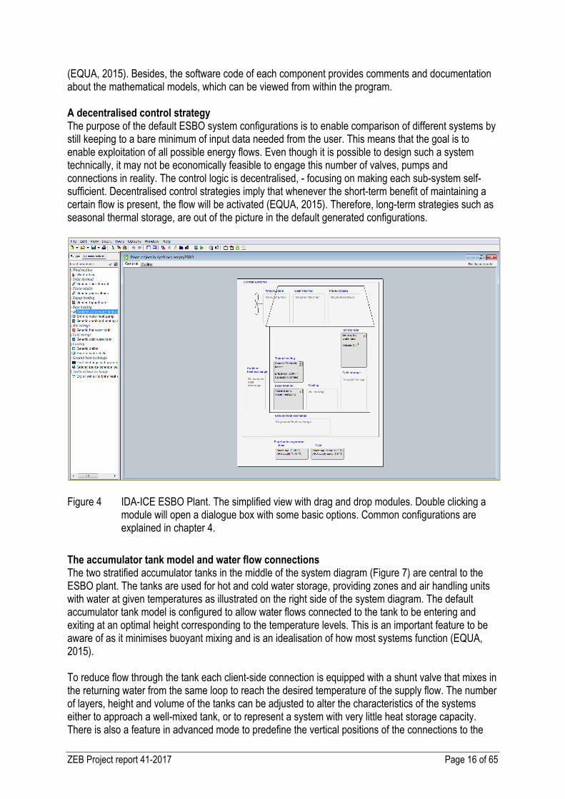
The process of creating diagrams and tables for performance comparison and analysis is nearly automated. The current version of the Excel templates is based on simulation results obtained using IDA-ICE 4.7. In the next chapters, the text passages specific to IDA-ICE are marked with blue text whereas the more general descriptions of the workflow use regular black text. | To use the Excel templates efficiently with IDA-ICE an output script was developed by EQUA. This script generates a result file with aggregated hourly data values from an annual simulation run in IDA-ICE. The result file has more than 8760 lines, one for each hour of the year. The columns are different parameters like hourly aggregated temperatures, mass flows and energy exchange between components. The available columns depend on the energy supply systems. For example, a result file from a simulation of an air to water heat pump and solar thermal heating panels will have more columns than a single auxiliary top heater.
Figure 6 Formatted result file imported into the main Excel sheet. The number and type of columns
are dependent on the type of system and the check boxes ticked in the list of output objects (step 2).
7 Selecting between electricity, fuel or district heating to be included in the delivered energy meter reporting.
ZEB Project report 41-2017 Page 19 of 65
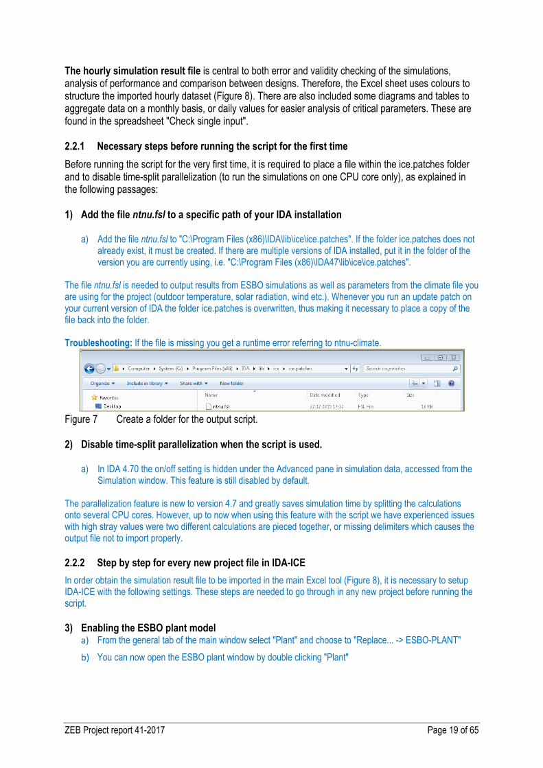
The hourly simulation result file is central to both error and validity checking of the simulations, analysis of performance and comparison between designs. Therefore, the Excel sheet uses colours to structure the imported hourly dataset (Figure 8). There are also included some diagrams and tables to aggregate data on a monthly basis, or daily values for easier analysis of critical parameters. These are found in the spreadsheet "Check single input". 2.2.1 Necessary steps before running the script for the first time
Before running the script for the very first time, it is required to place a file within the ice.patches folder and to disable time-split parallelization (to run the simulations on one CPU core only), as explained in the following passages: 1) Add the file ntnu.fsl to a specific path of your IDA installation
a) Add the file ntnu.fsl to "C:\Program Files (x86)\IDA\lib\ice\ice.patches". If the folder ice.patches does not
already exist, it must be created. If there are multiple versions of IDA installed, put it in the folder of the version you are currently using, i.e. "C:\Program Files (x86)\IDA47\lib\ice\ice.patches".
The file ntnu.fsl is needed to output results from ESBO simulations as well as parameters from the climate file you are using for the project (outdoor temperature, solar radiation, wind etc.). Whenever you run an update patch on your current version of IDA the folder ice.patches is overwritten, thus making it necessary to place a copy of the file back into the folder. Troubleshooting: If the file is missing you get a runtime error referring to ntnu-climate.
Figure 7 Create a folder for the output script. 2) Disable time-split parallelization when the script is used.
a) In IDA 4.70 the on/off setting is hidden under the Advanced pane in simulation data, accessed from the
Simulation window. This feature is still disabled by default. The parallelization feature is new to version 4.7 and greatly saves simulation time by splitting the calculations onto several CPU cores. However, up to now when using this feature with the script we have experienced issues with high stray values were two different calculations are pieced together, or missing delimiters which causes the output file not to import properly. 2.2.2 Step by step for every new project file in IDA-ICE
In order obtain the simulation result file to be imported in the main Excel tool (Figure 8), it is necessary to setup IDA-ICE with the following settings. These steps are needed to go through in any new project before running the script. 3) Enabling the ESBO plant model
a) From the general tab of the main window select "Plant" and choose to "Replace... -> ESBO-PLANT"
b) You can now open the ESBO plant window by double clicking "Plant"
ZEB Project report 41-2017 Page 20 of 65
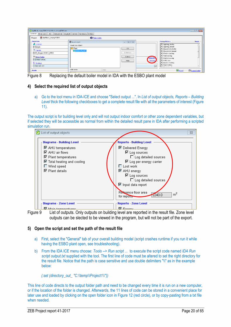
Figure 8 Replacing the default boiler model in IDA with the ESBO plant model
4) Select the required list of output objects
a) Go to the tool menu in IDA-ICE and choose "Select output ...". In List of output objects, Reports – Building
Level thick the following checkboxes to get a complete result file with all the parameters of interest (Figure 11).
The output script is for building level only and will not output indoor comfort or other zone dependent variables, but if selected they will be accessible as normal from within the detailed result pane in IDA after performing a scripted simulation run.
Figure 9 List of outputs. Only outputs on building level are reported in the result file. Zone level
outputs can be slected to be viewed in the program, but will not be part of the export. 5) Open the script and set the path of the result file
a) First, select the "General" tab of your overall building model (script crashes runtime if you run it while
having the ESBO plant open, see troubleshooting).
b) From the IDA ICE menu choose: Tools --> Run script ... to execute the script code named IDA Run script output.txt supplied with the tool. The first line of code must be altered to set the right directory for the result file. Notice that the path is case sensitive and use double delimiters "\\" as in the example below: (:set (directory_out_ "C:\\temp\\Project1\\"))
This line of code directs to the output folder path and need to be changed every time it is run on a new computer, or if the location of the folder is changed. Afterwards, the 11 lines of code can be stored in a convenient place for later use and loaded by clicking on the open folder icon in Figure 12 (red circle), or by copy-pasting from a txt file when needed.
ZEB Project report 41-2017 Page 21 of 65
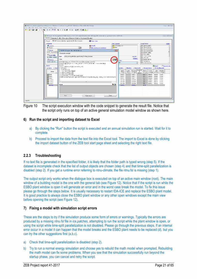
Figure 10 The script execution window with the code snippet to generate the result file. Notice that
the script only runs on top of an active general simulation model window as shown here. 6) Run the script and importing dataset to Excel
a) By clicking the "Run" button the script is executed and an annual simulation run is started. Wait for it to
complete.
b) Proceed to import the data from the text file into the Excel tool. The import to Excel is done by clicking the import dataset button of the ZEB tool start page sheet and selecting the right text file.
2.2.3 Troubleshooting
If no text file is generated in the specified folder, it is likely that the folder path is typed wrong (step 5). If the dataset is incomplete check that the list of output objects are chosen (step 4) and that time-split parallelization is disabled (step 2). If you get a runtime error referring to ntnu-climate, the file ntnu.fsl is missing (step 1). The output script only works when the dialogue box is executed on top of an active main window (root). The main window of a building model is the one with the general tab (see Figure 12). Notice that if the script is run while the ESBO plant window is open it will generate an error and in the worst case break the model. To fix this issue please go through the steps below. It is usually necessary to restart IDA-ICE and replace the ESBO plant model. It is good practice to always close the ESBO plant window or any other open windows except the main view before opening the script (see Figure 12). 7) Fixing a model with simulation script errors
These are the steps to try if the simulation produce some form of errors or warnings. Typically the errors are produced by a missing ntnu.fsl file in ice.patches, attempting to run the script while the plant window is open, or using the script while time-split parallelization is not disabled. Please go through the previous steps. If an internal error occur in a model it can happen that the model breaks and the ESBO plant needs to be replaced (d), but you can try the other suggestions first (a,b,c). a) Check that time-split parallelization is disabled (step 2).
b) Try to run a normal energy simulation and choose yes to rebuild the math model when prompted. Rebuilding the math model can fix some problems. When you see that the simulation successfully run beyond the startup phase, you can cancel and retry the script.

ZEB Project report 41-2017 Page 22 of 65
c) You should also try restarting IDA, or rebooting if you encounter an internal error.
d) If the above does not help, replacing the ESBO plant with an empty ESBO plant model can fix most problems, but you loose the current plant configuration (Replace -> Plant -> ESBO-PLANT).
2.3 Workflow diagram
See next page.

ZEB Project report 41-2017 Page 23 of 65
Figure 11 Workflow diagram and indication of where in the process Excel support tools are available

ZEB Project report 41-2017 Page 24 of 65
3. Building Load
The goal of the first section is to define the building model and details of building operation to establish a realistic heating demand profile under the right conditions. This includes a systematic approach to modelling largely based on the general methodology in NS 3031 and the process guideline built into IDA-ICE8.
OUTCOME: Daily or hourly load profile graphs; hourly power, energy demand and outdoor temperature, pinpointing max. and min. design temperatures. Complete diagrams can be found at the end of this chapter, in section 3.6. Load graph.
Example of building load figure.
REQUIRED STEPS: Before performing a whole year energy analysis, which creates the required data to create load profile graphs, it is necessary to go through the sub chapters:
Error! Reference source not found. Define building geometry and zoning
3.2 Set building envelope - Envelope components, Thermal bridges, Infiltration
3.3 Set building services - Ventilation System, Replace ideal zone heaters, User loads
3.4 Replace ESBO plant and run simulation for net energy (energy need) - Distribution temperature levels and distribution losses
3.5 Check comfort and net energy
8 The process guide is a feature of IDA-ICE, essentially a list of modelling tasks in a recommended order, i.e. starting with "building CAD geometry". Each task has a field to leave comments about the task, and four buttons to mark if the task is under work, completed, verified by someone (approved), or if it is simply not required for the current project.
-10
-5
0
5
10
15
20
25
30
0 %
10 %
20 %
30 %
40 %
50 %
60 %
70 %
80 %
90 %
100 %
0 1000 2000 3000 4000 5000 6000 7000 8000
Tem
pera
ture
[°C]
Cove
rage
fact
or [%
]
hour
Load curve (Heating and DHW)
Power (%)
Energy (%)
T_amb (°C)
Tamb-min,max [°C]-7.7 27.4
Heating + DHW[kWh/(m2a)]
PNet [W/m2] 12
11 30
ZEB Project report 41-2017 Page 25 of 65
3.1 Define building geometry and zoning
To achieve the goal of zero emissions form, function, material use and local site adaption needs to be optimised. Very low heat losses, good use of daylight and efficient use of ventilation must be planned well in the beginning of a project. These goals are linked to the organisation of functions and user accept of variations in daylight, temperatures, ventilation or other factors. All of these characteristics are important from the early stage of the design process and influence the choice and detailing of HVAC and other energy supply systems. The Norwegian energy calculation method technical supplement to NS 3031 give recommendations on how BPS models can be zoned according to solar exposure, use, operation, technical systems and other aspects that influence the thermal energy balance of the building. Another source that give recommendations on zoning procedures is the forthcoming overarching EPB standard ISO 52000-1 / prEN 16503.
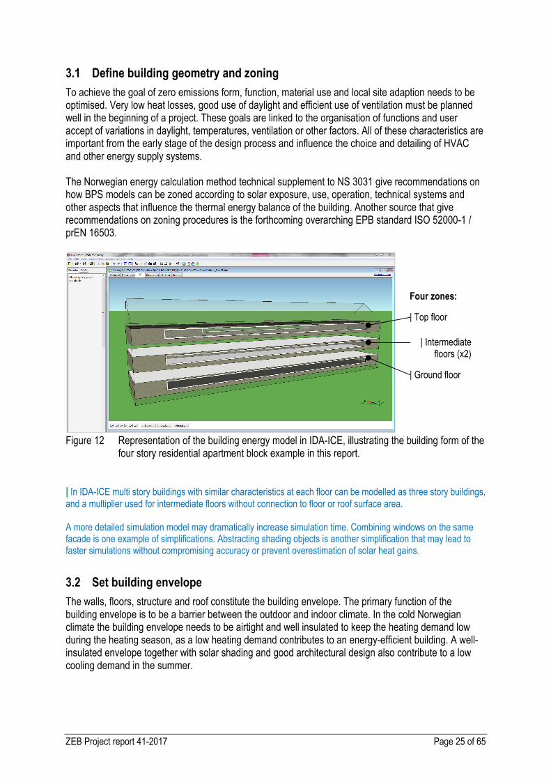
Figure 12 Representation of the building energy model in IDA-ICE, illustrating the building form of the
four story residential apartment block example in this report. | In IDA-ICE multi story buildings with similar characteristics at each floor can be modelled as three story buildings, and a multiplier used for intermediate floors without connection to floor or roof surface area. A more detailed simulation model may dramatically increase simulation time. Combining windows on the same facade is one example of simplifications. Abstracting shading objects is another simplification that may lead to faster simulations without compromising accuracy or prevent overestimation of solar heat gains.
3.2 Set building envelope
The walls, floors, structure and roof constitute the building envelope. The primary function of the building envelope is to be a barrier between the outdoor and indoor climate. In the cold Norwegian climate the building envelope needs to be airtight and well insulated to keep the heating demand low during the heating season, as a low heating demand contributes to an energy-efficient building. A well-insulated envelope together with solar shading and good architectural design also contribute to a low cooling demand in the summer.
| Top floor
| Intermediate floors (x2)
| Ground floor
Four zones:
ZEB Project report 41-2017 Page 26 of 65
3.2.1 Envelope components
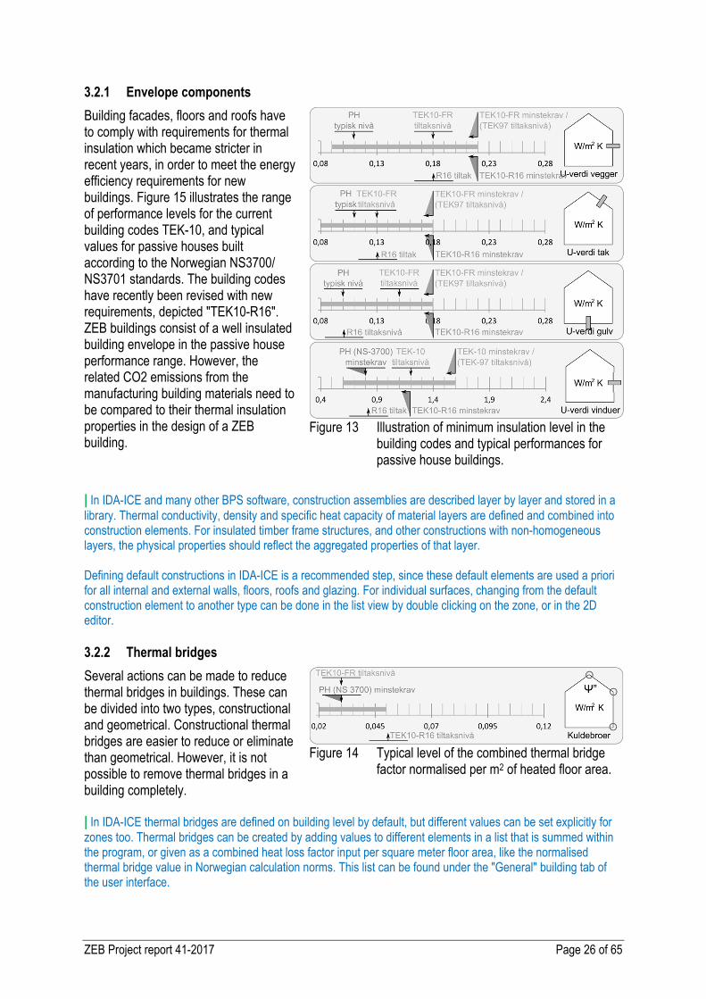
Building facades, floors and roofs have to comply with requirements for thermal insulation which became stricter in recent years, in order to meet the energy efficiency requirements for new buildings. Figure 15 illustrates the range of performance levels for the current building codes TEK-10, and typical values for passive houses built according to the Norwegian NS3700/ NS3701 standards. The building codes have recently been revised with new requirements, depicted "TEK10-R16". ZEB buildings consist of a well insulated building envelope in the passive house performance range. However, the related CO2 emissions from the manufacturing building materials need to be compared to their thermal insulation properties in the design of a ZEB building.
Figure 13 Illustration of minimum insulation level in the building codes and typical performances for passive house buildings.
| In IDA-ICE and many other BPS software, construction assemblies are described layer by layer and stored in a library. Thermal conductivity, density and specific heat capacity of material layers are defined and combined into construction elements. For insulated timber frame structures, and other constructions with non-homogeneous layers, the physical properties should reflect the aggregated properties of that layer. Defining default constructions in IDA-ICE is a recommended step, since these default elements are used a priori for all internal and external walls, floors, roofs and glazing. For individual surfaces, changing from the default construction element to another type can be done in the list view by double clicking on the zone, or in the 2D editor. 3.2.2 Thermal bridges
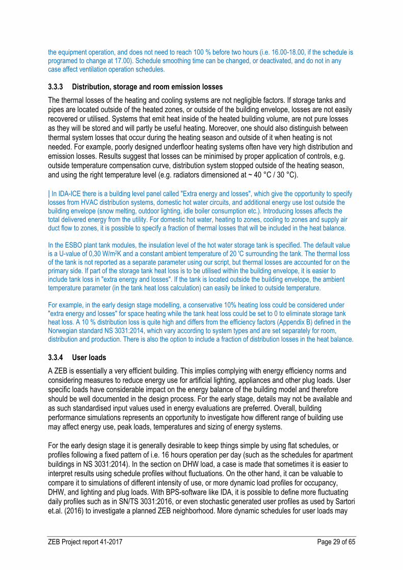
Several actions can be made to reduce thermal bridges in buildings. These can be divided into two types, constructional and geometrical. Constructional thermal bridges are easier to reduce or eliminate than geometrical. However, it is not possible to remove thermal bridges in a building completely.
Figure 14 Typical level of the combined thermal bridge factor normalised per m2 of heated floor area.
| In IDA-ICE thermal bridges are defined on building level by default, but different values can be set explicitly for zones too. Thermal bridges can be created by adding values to different elements in a list that is summed within the program, or given as a combined heat loss factor input per square meter floor area, like the normalised thermal bridge value in Norwegian calculation norms. This list can be found under the "General" building tab of the user interface.

ZEB Project report 41-2017 Page 27 of 65
3.2.3 Infiltration
Air tightness of the building envelope is important to prevent heat loss. Air tightness is also important to the envelope moisture performance. The building industry is steadily improving their products and develop new solutions, e.g. to reach air tightness below 0.6 m3/(m3h) as in the passive house requirement at 50 Pa pressure difference (Figure 17).
Figure 15 Infiltration typical performance levels
| In IDA-ICE infiltration is also defined on building level by default, but can be overridden per zone. There are options to account for wind driven flow and to distribute leakages proportionally to the surface area, volume, or floor area of each zone. For wind driven infiltration (which is usually preferred over fixed flow), it is necessary to specify the external pressure coefficients of facades and other exposed surfaces. It may also be necessary to define internal leakage paths such as doors or cracks between zones to account for wind driven flow. Especially if there are several zones on the same floor with different facade orientations.
3.3 Set building services
Energy-efficient buildings with super-insulated building envelopes and zero emission ambitions introduces both opportunities and challenges when it comes to the design of building services. Building services for ZEB are not necessarily different, but with these guidelines we are particularly interested in the ability to compare different technologies and the integration into the building. 3.3.1 Ventilation System
Ventilation is necessary to maintain a good indoor air quality, but often also to remove excess heat or to supply heat for space heating. In cold climates it will always represent a heat loss and require use of energy, but how much depends on which technical solutions are used and how well it is designed. The minimum requirements for ventilation are regulated in building codes and working environment legislation. The ventilation method and room ventilation effectiveness affect the required ventilation rates. Because the user load will often vary during a day, it may be possible to demand control ventilation. There are two main strategies, either using sensors modulating the airflow in real-time with a VAV-system, or switching the flow between different pre-scheduled levels in the course of the day using a timer with a CAV-system. Both strategies can be modulated in a BPS software like IDA-ICE. | Figure 18 shows the main structure of the AHU, with the fans, the heat exchanger and the heating and cooling coils (cooling coil not used in these simulations). Central parameters are choosing the supply air set point temperature, specific fan power of supply and extract fans, and the heat recovery efficiency.

ZEB Project report 41-2017 Page 28 of 65
Figure 16 Schematic of the Air Handling Unit, AHU, in IDA ICE.
The air handling units in IDA-ICE are by default of unlimited capacity. However when the ESBO plant is enabled, the ability to provide conditioned air to the set point temperature will be affected by the type and capacity of the heating and cooling system. For example, if no cooling system is defined in ESBO plant, the supply air will not be cooled in the summer. As an additional measure, the efficiency of the cooling coil in the ventilation plant can be set to 0 to disable cooling (Figure 10). We choose a constant air volume (CAV) system for the apartment building that supplies conditioned fresh air to the zones at 18°C throughout the year; a typical ventilation system in Norwegian new built residential units. Since there is no active cooling, in summer the supply temperature will exceed 18°C at times. To make sure the script includes all the data for HVAC, it is advisable to keep the default pre-defined energy meters for fans, coils and heat recovery units. 3.3.2 Zones heating (switch ideal heaters to PI control)
The space-heating system needs to be able to provide thermal comfort during very cold periods without significant contributions from internal gains and passive solar heat. In traditional system designs, it is assumed that one should be able to ensure thermal comfort with a minimum outdoor temperature applied continuously under steady-state conditions, (e.g. -20 °C in Oslo). This is far from the everyday operating conditions, and may lead to over-dimensioning of heaters and generation systems. When evaluating the nominal space heating power, design choices should be discussed properly as part of the risk assessment. It should be agreed if internal gains should be included or not, if intermittent heating such as night set-back is necessary and the design outdoor temperature should be evaluated. | For zone heating replace the default heating and cooling room units with a Heating/cooling panel (hc-panel). It is necessary to set the design heating power (Watt). The hc-panel has a default PI controlled thermostat and an average temperature difference of 20 °C between room and heating panel, with a 10 °C hot water temperature drop over the unit at design conditions. In other words, this is a typical radiator dimensioned at ~ 40 °C / 30 °C. For our application we have set the cooling design power to 0 Watt. Another simulation parameter in IDA-ICE that has some influence over intermittent power for heating and cooling is the degree of automatic schedule smoothing. Since operating schedules for occupant presence, equipment, lighting, shading and window operation may introduce sharp transitions in the calculations, IDA-ICE has a default schedule smoothing of ±1 hour, to minimise problems and to lead to a faster computation time. A setting of 1 hour means that the software can activate the schedule at the hour before or after the expected starting/ending of
ZEB Project report 41-2017 Page 29 of 65
the equipment operation, and does not need to reach 100 % before two hours (i.e. 16.00-18.00, if the schedule is programed to change at 17.00). Schedule smoothing time can be changed, or deactivated, and do not in any case affect ventilation operation schedules. 3.3.3 Distribution, storage and room emission losses
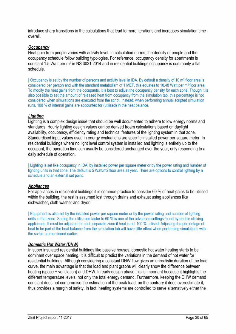
The thermal losses of the heating and cooling systems are not negligible factors. If storage tanks and pipes are located outside of the heated zones, or outside of the building envelope, losses are not easily recovered or utilised. Systems that emit heat inside of the heated building volume, are not pure losses as they will be stored and will partly be useful heating. Moreover, one should also distinguish between thermal system losses that occur during the heating season and outside of it when heating is not needed. For example, poorly designed underfloor heating systems often have very high distribution and emission losses. Results suggest that losses can be minimised by proper application of controls, e.g. outside temperature compensation curve, distribution system stopped outside of the heating season, and using the right temperature level (e.g. radiators dimensioned at ~ 40 °C / 30 °C). | In IDA-ICE there is a building level panel called "Extra energy and losses", which give the opportunity to specify losses from HVAC distribution systems, domestic hot water circuits, and additional energy use lost outside the building envelope (snow melting, outdoor lighting, idle boiler consumption etc.). Introducing losses affects the total delivered energy from the utility. For domestic hot water, heating to zones, cooling to zones and supply air duct flow to zones, it is possible to specify a fraction of thermal losses that will be included in the heat balance. In the ESBO plant tank modules, the insulation level of the hot water storage tank is specified. The default value is a U-value of 0,30 W/m2K and a constant ambient temperature of 20 'C surrounding the tank. The thermal loss of the tank is not reported as a separate parameter using our script, but thermal losses are accounted for on the primary side. If part of the storage tank heat loss is to be utilised within the building envelope, it is easier to include tank loss in "extra energy and losses". If the tank is located outside the building envelope, the ambient temperature parameter (in the tank heat loss calculation) can easily be linked to outside temperature. For example, in the early design stage modelling, a conservative 10% heating loss could be considered under "extra energy and losses" for space heating while the tank heat loss could be set to 0 to eliminate storage tank heat loss. A 10 % distribution loss is quite high and differs from the efficiency factors (Appendix B) defined in the Norwegian standard NS 3031:2014, which vary according to system types and are set separately for room, distribution and production. There is also the option to include a fraction of distribution losses in the heat balance. 3.3.4 User loads
A ZEB is essentially a very efficient building. This implies complying with energy efficiency norms and considering measures to reduce energy use for artificial lighting, appliances and other plug loads. User specific loads have considerable impact on the energy balance of the building model and therefore should be well documented in the design process. For the early stage, details may not be available and as such standardised input values used in energy evaluations are preferred. Overall, building performance simulations represents an opportunity to investigate how different range of building use may affect energy use, peak loads, temperatures and sizing of energy systems. For the early design stage it is generally desirable to keep things simple by using flat schedules, or profiles following a fixed pattern of i.e. 16 hours operation per day (such as the schedules for apartment buildings in NS 3031:2014). In the section on DHW load, a case is made that sometimes it is easier to interpret results using schedule profiles without fluctuations. On the other hand, it can be valuable to compare it to simulations of different intensity of use, or more dynamic load profiles for occupancy, DHW, and lighting and plug loads. With BPS-software like IDA, it is possible to define more fluctuating daily profiles such as in SN/TS 3031:2016, or even stochastic generated user profiles as used by Sartori et.al. (2016) to investigate a planned ZEB neighborhood. More dynamic schedules for user loads may
ZEB Project report 41-2017 Page 30 of 65
introduce sharp transitions in the calculations that lead to more iterations and increases simulation time overall. Occupancy Heat gain from people varies with activity level. In calculation norms, the density of people and the occupancy schedule follow building typologies. For reference, occupancy density for apartments is constant 1.5 Watt per m2 in NS 3031:2014 and in residential buildings occupancy is commonly a flat schedule. | Occupancy is set by the number of persons and activity level in IDA. By default a density of 10 m2 floor area is considered per person and with the standard metabolism of 1 MET, this equates to 10.48 Watt per m2 floor area. To modify the heat gains from the occupants, it is best to adjust the occupancy density for each zone. Though it is also possible to set the amount of released heat from occupancy from the simulation tab, this percentage is not considered when simulations are executed from the script. Instead, when performing annual scripted simulation runs, 100 % of internal gains are accounted for (utilised) in the heat balance. Lighting Lighting is a complex design issue that should be well documented to adhere to low energy norms and standards. Hourly lighting design values can be derived froam calculations based on daylight availability, occupancy, efficiency rating and technical features of the lighting system in that zone. Standardised input values used in energy evaluations are specific installed power per square meter. In residential buildings where no light level control system is installed and lighting is entirely up to the occupant, the operation time can usually be considered unchanged over the year, only responding to a daily schedule of operation. | Lighting is set like occupancy in IDA, by installed power per square meter or by the power rating and number of lighting units in that zone. The default is 5 Watt/m2 floor area all year. There are options to control lighting by a schedule and an external set point. Appliances For appliances in residential buildings it is common practice to consider 60 % of heat gains to be utilised within the building, the rest is assumed lost through drains and exhaust using appliances like dishwasher, cloth washer and dryer. | Equipment is also set by the installed power per square meter or by the power rating and number of lighting units in that zone. Setting the utilisation factor to 60 % is one of the advanced settings found by double clicking appliances. It must be adjusted for each separate zone if heat is not 100 % utilised. Adjusting the percentage of heat to be part of the heat balance from the simulation tab will have little effect when performing simulations with the script, as mentioned earlier. Domestic Hot Water (DHW) In super insulated residential buildings like passive houses, domestic hot water heating starts to be dominant over space heating. It is difficult to predict the variations in the demand of hot water for residential buildings. Although considering a constant DHW flow gives an unrealistic duration of the load curve, the main advantage is that the load and plant graphs will clearly show the difference between heating (space + ventilation) and DHW. In early design phase this is important because it highlights the different temperature levels, not only the total energy demand. Furthermore, keeping the DHW demand constant does not compromise the estimation of the peak load; on the contrary it does overestimate it, thus provides a margin of safety. In fact, heating systems are controlled to serve alternatively either the
ZEB Project report 41-2017 Page 31 of 65
heating load or the DHW load9 (with priority on the latter), so that the peak load is only given by the heating demand. Therefore, considering the DHW always present at a (low) constant value does provide a somewhat overestimated thermal peak load. | When defining hot water use, there are different options which affect the demand profiles. It is possible to define a daily profile as suggested in SN/TS 3031:2016 (table A.2, apartment building), or use a constant draw as recommended in the text above for early design. According to the current norm, the demand is set to 3.4 W/m2 at a constant rate which adds up to 29,8 kWh/m2 year (NS 3031:2014 table A.1, apartment building), whereas table A.2 in the supplement has reduced this value to 25 kWh/m2 year. In IDA, DHW demand can be set separately for each zone, or globally in different scales (litre/person day, W/m2, kWh/m2 year etc.) In any case, tap water is considered to be heated from 5 to 60 °C, with 55 °C temperature draw by default.
3.4 Replace ESBO plant and run simulation for net energy (energy need)
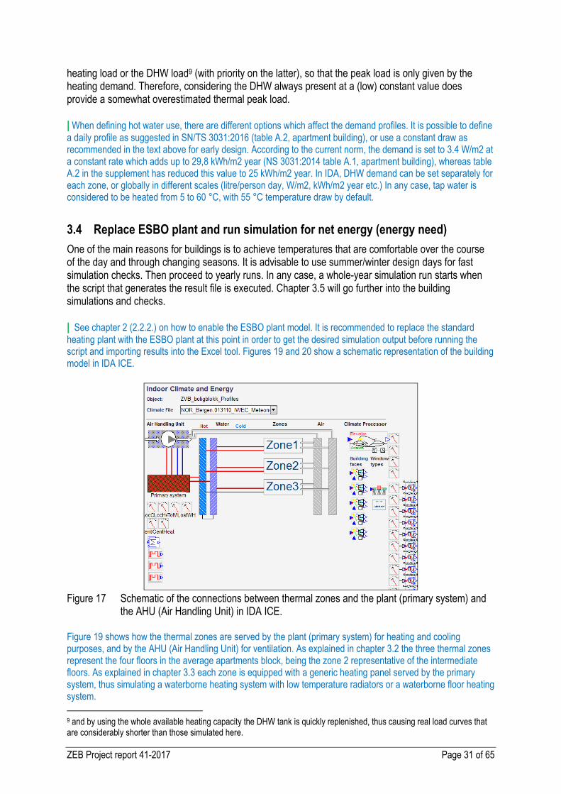
One of the main reasons for buildings is to achieve temperatures that are comfortable over the course of the day and through changing seasons. It is advisable to use summer/winter design days for fast simulation checks. Then proceed to yearly runs. In any case, a whole-year simulation run starts when the script that generates the result file is executed. Chapter 3.5 will go further into the building simulations and checks. | See chapter 2 (2.2.2.) on how to enable the ESBO plant model. It is recommended to replace the standard heating plant with the ESBO plant at this point in order to get the desired simulation output before running the script and importing results into the Excel tool. Figures 19 and 20 show a schematic representation of the building model in IDA ICE.
Figure 17 Schematic of the connections between thermal zones and the plant (primary system) and
the AHU (Air Handling Unit) in IDA ICE. Figure 19 shows how the thermal zones are served by the plant (primary system) for heating and cooling purposes, and by the AHU (Air Handling Unit) for ventilation. As explained in chapter 3.2 the three thermal zones represent the four floors in the average apartments block, being the zone 2 representative of the intermediate floors. As explained in chapter 3.3 each zone is equipped with a generic heating panel served by the primary system, thus simulating a waterborne heating system with low temperature radiators or a waterborne floor heating system. 9 and by using the whole available heating capacity the DHW tank is quickly replenished, thus causing real load curves that are considerably shorter than those simulated here.
ZEB Project report 41-2017 Page 32 of 65
3.4.1 Distribution temperatures
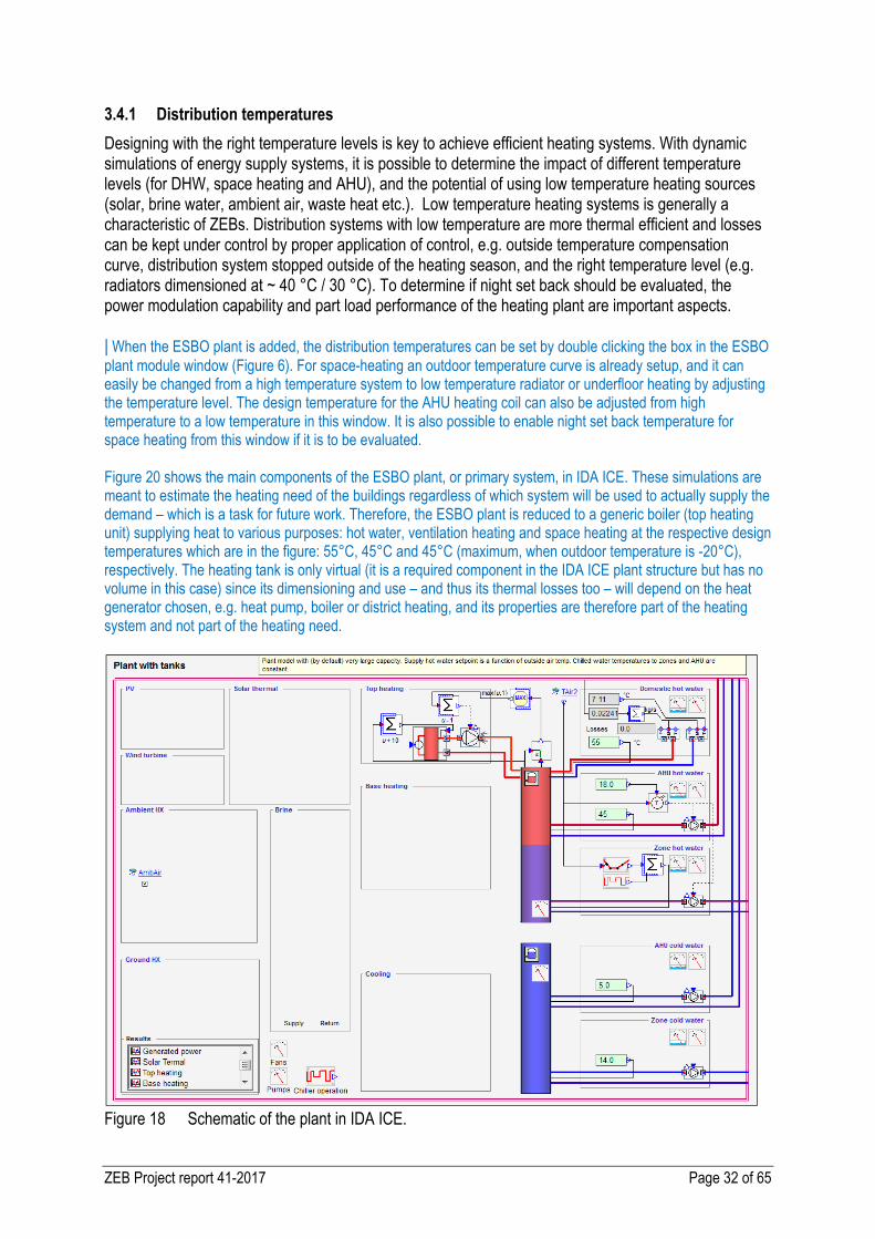
Designing with the right temperature levels is key to achieve efficient heating systems. With dynamic simulations of energy supply systems, it is possible to determine the impact of different temperature levels (for DHW, space heating and AHU), and the potential of using low temperature heating sources (solar, brine water, ambient air, waste heat etc.). Low temperature heating systems is generally a characteristic of ZEBs. Distribution systems with low temperature are more thermal efficient and losses can be kept under control by proper application of control, e.g. outside temperature compensation curve, distribution system stopped outside of the heating season, and the right temperature level (e.g. radiators dimensioned at ~ 40 °C / 30 °C). To determine if night set back should be evaluated, the power modulation capability and part load performance of the heating plant are important aspects. | When the ESBO plant is added, the distribution temperatures can be set by double clicking the box in the ESBO plant module window (Figure 6). For space-heating an outdoor temperature curve is already setup, and it can easily be changed from a high temperature system to low temperature radiator or underfloor heating by adjusting the temperature level. The design temperature for the AHU heating coil can also be adjusted from high temperature to a low temperature in this window. It is also possible to enable night set back temperature for space heating from this window if it is to be evaluated. Figure 20 shows the main components of the ESBO plant, or primary system, in IDA ICE. These simulations are meant to estimate the heating need of the buildings regardless of which system will be used to actually supply the demand – which is a task for future work. Therefore, the ESBO plant is reduced to a generic boiler (top heating unit) supplying heat to various purposes: hot water, ventilation heating and space heating at the respective design temperatures which are in the figure: 55°C, 45°C and 45°C (maximum, when outdoor temperature is -20°C), respectively. The heating tank is only virtual (it is a required component in the IDA ICE plant structure but has no volume in this case) since its dimensioning and use – and thus its thermal losses too – will depend on the heat generator chosen, e.g. heat pump, boiler or district heating, and its properties are therefore part of the heating system and not part of the heating need.
Figure 18 Schematic of the plant in IDA ICE.

ZEB Project report 41-2017 Page 33 of 65
3.5 Check comfort and net energy
To understand the energy flows of a building model, it is often useful to use a relatively short time period so that designers can focus on one set of weather phenomena at a time. To check that internal loads and solar gains are reasonable, a whole year energy simulation is recommended. Follow the workflow below and then use the script step-by-step as outlined in chapter 2 to generate a result file of a whole-year simulation. The result file can be imported into the Excel tool for further analysis. | In IDA-ICE there are several types of simulation. A heating load simulation is a good place to start and then heating, cooling and energy simulations (for a whole year) can be run for the same simulation period, or a custom simulation in a specific period of the year. 3.5.1 Thermal Comfort
Check thermal comfort by investigating room temperatures. | A heating load simulation can help with system sizing of the room heating and ventilation system. Issues with overheating in summer can be checked by using a cooling load simulation (see next section). 3.5.2 Air Quality
Check ventilation rates, or other indicators of air quality. Schedules for windows opening may be used to simulate the effect of natural ventilation in summer and prevent overheating. Even if active cooling is not considered, it is nonetheless preferable to avoid situations of overheating, e.g. with indoor temperatures above 30°C, as it may the case if the windows are simulated as always closed. On one hand this would look undesirable and/or unrealistic; on the other hand it may cause excessive rise of indoor temperatures in the swing season, April-May and September-October which gives an underestimated heating need. However, one should be aware of not running into other unrealistic simulation results, such as extremely high natural ventilation rates. This is the often the case when simulating opening of windows, especially by opening of windows in different facades in the same zone, like in cross ventilation. | In IDA ICE, when window ventilation is enabled with PI temperature control, the software tries to keep the indoor temperature setting, e.g. 26°C, by opening the windows. This may result in excessive air flow rates, e.g. up to 20 ach or more. A remedy to this is to associate windows opening control with a limiting schedule, e.g. a schedule which is always ON, thus allowing the opening to happen if need be as defined by the controller, but set to a value of 0.1 instead of 1. The right limiting value can be found case by case by trial and error, until the resulting air flow in the zones does not exceed ca. 5-6 ach in its maximum value10. Normally it is possible to achieve reasonable levels of the indoor temperature, e.g. below 28°C, with reasonable levels of natural air flow, at least in the Norwegian climate. This is due to the fact that in the presence of limitations on the amount of windows opening, the software will keep the windows open for a longer time, thus obtaining the desired cooling effect but avoid high spikes in the air flow values. 3.5.3 Heat loss and Net energy requirements check
Check that that the heat balance is reasonable. Check that internal loads and solar gains are correct through a whole year energy simulation. | From the simulation tab in IDA-ICE it is possible to set the percentage of internal gains (from occupants, lighting and equipment) to be included in the heat balance. However, by using the script to execute a whole year simulation, these settings are overlooked. Instead 100 % of internal gains are released to the zones.
10 A complete opening of windows in a room normally allows for a complete air change in 10-15 min, thus it is reasonable and realistic to accept maximum values of 5-6 ach.
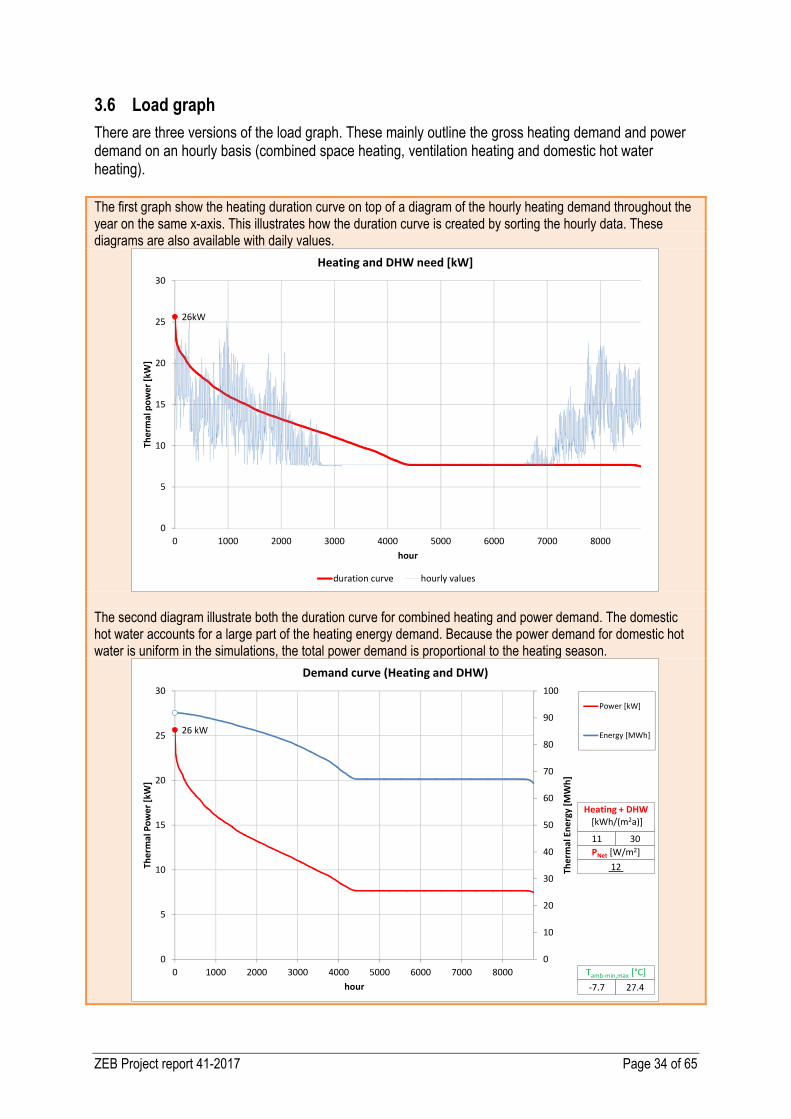
ZEB Project report 41-2017 Page 34 of 65
3.6 Load graph
There are three versions of the load graph. These mainly outline the gross heating demand and power demand on an hourly basis (combined space heating, ventilation heating and domestic hot water heating). The first graph show the heating duration curve on top of a diagram of the hourly heating demand throughout the year on the same x-axis. This illustrates how the duration curve is created by sorting the hourly data. These diagrams are also available with daily values.
The second diagram illustrate both the duration curve for combined heating and power demand. The domestic hot water accounts for a large part of the heating energy demand. Because the power demand for domestic hot water is uniform in the simulations, the total power demand is proportional to the heating season.
26kW
0
5
10
15
20
25
30
0 1000 2000 3000 4000 5000 6000 7000 8000
Ther
mal
pow
er [k
W]
hour
Heating and DHW need [kW]
duration curve hourly values
26 kW
0
10
20
30
40
50
60
70
80
90
100
0
5
10
15
20
25
30
0 1000 2000 3000 4000 5000 6000 7000 8000
Ther
mal
Ene
rgy
[MW
h]
Ther
mal
Pow
er [k
W]
hour
Demand curve (Heating and DHW)
Power [kW]
Energy [MWh]
Tamb-min,max [°C]-7.7 27.4
Heating + DHW[kWh/(m2a)]
PNet [W/m2] 12
11 30
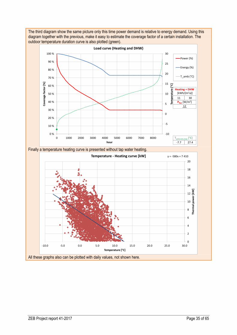
ZEB Project report 41-2017 Page 35 of 65
The third diagram show the same picture only this time power demand is relative to energy demand. Using this diagram together with the previous, make it easy to estimate the coverage factor of a certain installation. The outdoor temperature duration curve is also plotted (green).
Finally a temperature heating curve is presented without tap water heating.
All these graphs also can be plotted with daily values, not shown here.
-10
-5
0
5
10
15
20
25
30
0 %
10 %
20 %
30 %
40 %
50 %
60 %
70 %
80 %
90 %
100 %
0 1000 2000 3000 4000 5000 6000 7000 8000
Tem
pera
ture
[°C]
Cove
rage
fact
or [%
]
hour
Load curve (Heating and DHW)
Power (%)
Energy (%)
T_amb (°C)
Tamb-min,max [°C]-7.7 27.4
Heating + DHW[kWh/(m2a)]
PNet [W/m2] 12
11 30
y = -580x + 7 410
0
2
4
6
8
10
12
14
16
18
20
-10.0 -5.0 0.0 5.0 10.0 15.0 20.0 25.0 30.0
Ther
mal
pow
er [k
W]
Temperature [°C]
Temperature - Heating curve [kW]
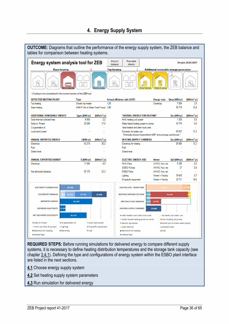
ZEB Project report 41-2017 Page 36 of 65
4. Energy Supply System
OUTCOME: Diagrams that outline the performance of the energy supply system, the ZEB balance and tables for comparison between heating systems.
REQUIRED STEPS: Before running simulations for delivered energy to compare different supply systems, it is necessary to define heating distribution temperatures and the storage tank capacity (see chapter 3.4.1). Defining the type and configurations of energy system within the ESBO plant interface are listed in the next sections.
4.1 Choose energy supply system
4.2 Set heating supply system parameters
4.3 Run simulation for delivered energy

ZEB Project report 41-2017 Page 37 of 65
4.1 Choose energy supply system
Different type of energy supply systems applicable for ZEB's are presented as well as how they can be modelled using the ESBO plant model. A brief description of the conceptual layout of the plant, the solar thermal, base heating and top heating slots can be found in chapter 1.3. | If the ESBO plant has not already been added to the model it is necessary to do so (chapter 3.4). Then the type of energy supply system can be chosen among the preconfigured types of top heaters, base heaters, solar thermal, PV panels, or other modules. It is not always required to build the plant models system diagram. Simple drag and drop or double clicking the modules to make adjustments to the temperature levels for space heating, the tank capacity and the module specific parameters, which are available without the 'build plant option'. The principles for the configuration and control of the default ESBO systems are described in the manual (EQUA, 2015). 4.1.1 District heating
A district heating (DH) system produces, delivers and distributes hot water to external users. The use of DH requires that the building has installed a waterborne distribution system. | In IDA-ICE district heating can be introduced by setting a top heater with unlimited capacity and an efficiency of 0.88 when using radiators and 0.84 when using floor heating (according to NS 3031:2014). For a top heating system the type of energy carrier can be selected from a list, so for district heat this should be set to “district”. District heating is the easiest heating system to set up in IDA-ICE. 4.1.2 Bio-boiler
Biomass is an organic, carbon-based material that reacts with oxygen in combustion to release heat. Woody biomass is the most commonly used fuel. It is considered renewable if the carbon emissions released in the atmosphere by burning the biomass are compensated by the carbon stored in the regrowth. | In IDA-ICE the bio boiler can be introduced by choosing a combined heating and power base heater with zero electricity production efficiency. The heating efficiency will be set to the efficiency of the boiler. Maximum heating capacity also has to be choosen. In version 4.51 of IDA-ICE there was some problems with the control system when using a bio boiler/CHP in combination with an electric top heater. The boiler would mostly work on half the maximum capacity even though the energy demand was twice as large. Instead the top heater would cover the rest of the load. A simple solution to this problem was to double the maximum heating capacity of the boiler in IDA-ICE compared to the real maximum capacity. The boiler would then perform according to the actual boiler, and thereby cover most of the heating load alone. 4.1.3 Combined Heat and Power (CHP)
Combined heat and power, also known as cogeneration, provides very high efficiency by combining heat and electricity production, but unfortunately only exits in small scale on the Norwegian marked. | As mentioned above both bio boilers and the CHP can use the same model in IDA-ICE, the combined heating and power base heater-model. For CHP both a heating efficiency and an electricity production efficiency must be chosen, as well as the total heating capacity. The problem with the control system also applies to CHP, making the boiler run on low load in combination with the top electric heater. The simplest solution is the same as for the bio boiler, to over dimension the boiler so it will have a more realistic performance.
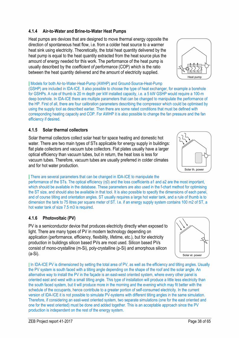
ZEB Project report 41-2017 Page 38 of 65
4.1.4 Air-to-Water and Brine-to-Water Heat Pumps
Heat pumps are devices that are designed to move thermal energy opposite the direction of spontaneous heat flow, i.e. from a colder heat source to a warmer heat sink using electricity. Theoretically, the total heat quantity delivered by the heat pump is equal to the heat quantity extracted from the heat source plus the amount of energy needed for this work. The performance of the heat pump is usually described by the coefficient of performance (COP) which is the ratio between the heat quantity delivered and the amount of electricity supplied. | Models for both Air-to-Water-Heat-Pump (AWHP) and Ground-Source-Heat-Pump (GSHP) are included in IDA-ICE. It also possible to choose the type of heat exchanger, for example a borehole for GSHPs. A rule of thumb is 20 m depth per kW installed capacity, i.e. a 5 kW GSHP would require a 100-m deep borehole. In IDA-ICE there are multiple parameters that can be changed to manipulate the performance of the HP. First of all, there are four calibration parameters describing the compressor which could be optimised by using the supply tool as described earlier. Then there are some rated conditions that must be defined with corresponding heating capacity and COP. For AWHP it is also possible to change the fan pressure and the fan efficiency if desired. 4.1.5 Solar thermal collectors
Solar thermal collectors collect solar heat for space heating and domestic hot water. There are two main types of STs applicable for energy supply in buildings: flat plate collectors and vacuum tube collectors. Flat plates usually have a larger optical efficiency than vacuum tubes, but in return, the heat loss is less for vacuum tubes. Therefore, vacuum tubes are usually preferred in colder climates and for hot water production. | There are several parameters that can be changed in IDA-ICE to manipulate the performance of the STs. The optical efficiency (η0) and the loss coefficients a1 and a2 are the most important, which should be available in the database. These parameters are also used in the f-chart method for optimising the ST size, and should also be available in that tool. It is also possible to specify the dimensions of each panel, and of course tilting and orientation angles. ST usually requires a large hot water tank, and a rule of thumb is to dimension the tank to 75 litres per square meter of ST. I.e. if an energy supply system contains 100 m2 of ST, a hot water tank of size 7.5 m3 is required. 4.1.6 Photovoltaic (PV)
PV is a semiconductor device that produces electricity directly when exposed to light. There are many types of PV in modern technology depending on application (performance, efficiency, flexibility, lifetime, etc.), but for electricity production in buildings silicon based PVs are most used. Silicon based PVs consist of mono-crystalline (m-Si), poly-crystalline (p-Si) and amorphous silicon (a-Si). | In IDA-ICE PV is dimensioned by setting the total area of PV, as well as the efficiency and tilting angles. Usually the PV system is south faced with a tilting angle depending on the shape of the roof and the solar angle. An alternative way to install the PV in the façade is an east-west oriented system, where every other panel is oriented east and west with a small tilting angle. This type of installation will produce a little less electricity than the south faced system, but it will produce more in the morning and the evening which may fit better with the schedule of the occupants, hence contribute to a greater portion of self-consumed electricity. In the current version of IDA-ICE it is not possible to simulate PV-systems with different tilting angles in the same simulation. Therefore, if considering an east-west oriented system, two separate simulations (one for the east oriented and one for the west oriented) must be done and added together. This is an acceptable approach since the PV production is independent on the rest of the energy system.
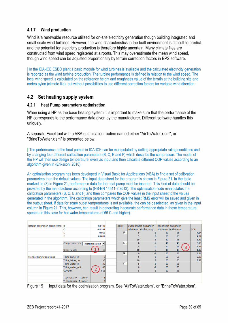
ZEB Project report 41-2017 Page 39 of 65
4.1.7 Wind production
Wind is a renewable resource utilised for on-site electricity generation though building integrated and small-scale wind turbines. However, the wind characteristics in the built environment is difficult to predict and the potential for electricity production is therefore highly uncertain. Many climate files are constructed from wind speed registered at airports. This may overestimate the mean wind speed, though wind speed can be adjusted proportionally by terrain correction factors in BPS software. | In the IDA-ICE ESBO plant a basic module for wind turbines is available and the calculated electricity generation is reported as the wind turbine production. The turbine performance is defined in relation to the wind speed. The local wind speed is calculated on the reference height and roughness value of the terrain at the building site and meteo pylon (climate file), but without possibilities to use different correction factors for variable wind direction.
4.2 Set heating supply system
4.2.1 Heat Pump parameters optimisation
When using a HP as the base heating system it is important to make sure that the performance of the HP corresponds to the performance data given by the manufacturer. Different software handles this uniquely. A separate Excel tool with a VBA optimisation routine named either "AirToWater.xlsm", or "BrineToWater.xlsm" is presented below. | The performance of the heat pumps in IDA-ICE can be manipulated by setting appropriate rating conditions and by changing four different calibration parameters (B, C, E and F) which describe the compressor. The model of the HP will then use design temperature levels as input and then calculate different COP values according to an algorithm given in (Eriksson, 2010). An optimisation program has been developed in Visual Basic for Applications (VBA) to find a set of calibration parameters than the default values. The input data sheet for the program is shown in Figure 21. In the table marked as (3) in Figure 21, performance data for the heat pump must be inserted. This kind of data should be provided by the manufacturer according to (NS-EN 14511-2:2013). The optimisation code manipulates the calibration parameters (B, C, E and F) and then compares the COP values in the input sheet to the values generated in the algorithm. The calibration parameters which give the least RMS error will be saved and given in the output sheet. If data for some outlet temperatures is not available, the can be deselected, as given in the input column in Figure 21. This, however, can result in generating inaccurate performance data in these temperature spectra (in this case for hot water temperatures of 65 C and higher).
Figure 19 Input data for the optimisation program. See "AirToWater.xlsm", or "BrineToWater.xlsm".
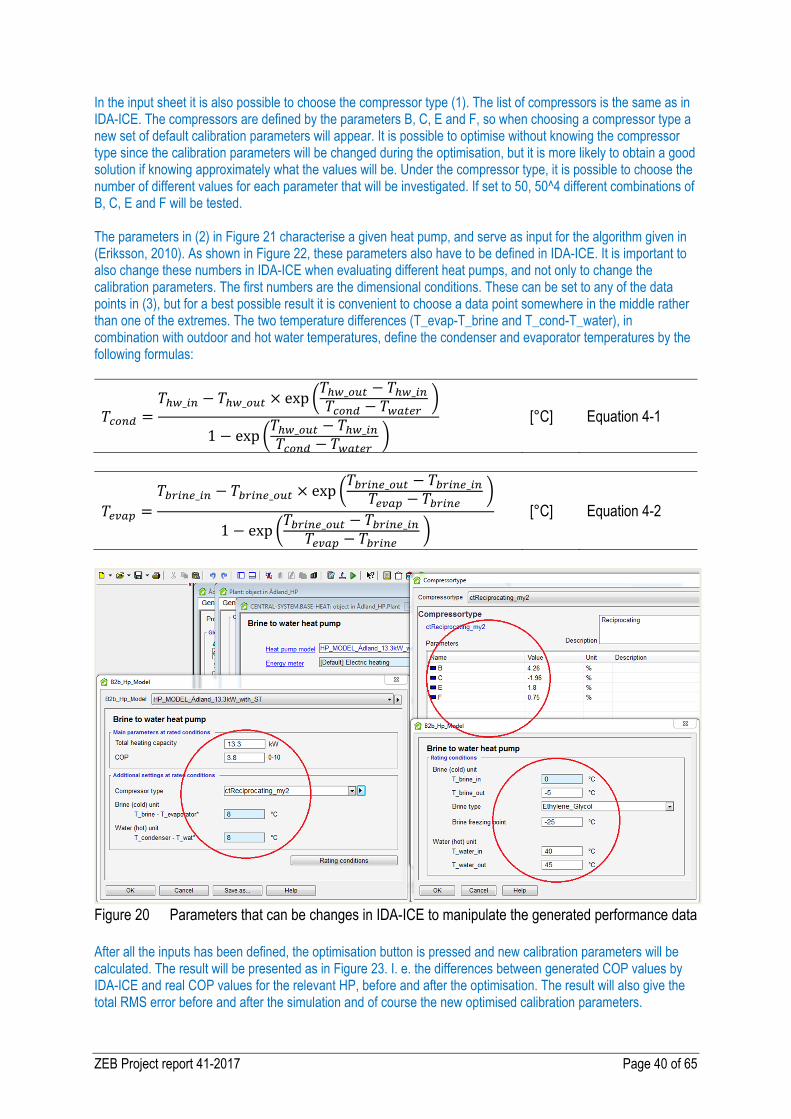
ZEB Project report 41-2017 Page 40 of 65
In the input sheet it is also possible to choose the compressor type (1). The list of compressors is the same as in IDA-ICE. The compressors are defined by the parameters B, C, E and F, so when choosing a compressor type a new set of default calibration parameters will appear. It is possible to optimise without knowing the compressor type since the calibration parameters will be changed during the optimisation, but it is more likely to obtain a good solution if knowing approximately what the values will be. Under the compressor type, it is possible to choose the number of different values for each parameter that will be investigated. If set to 50, 50^4 different combinations of B, C, E and F will be tested. The parameters in (2) in Figure 21 characterise a given heat pump, and serve as input for the algorithm given in (Eriksson, 2010). As shown in Figure 22, these parameters also have to be defined in IDA-ICE. It is important to also change these numbers in IDA-ICE when evaluating different heat pumps, and not only to change the calibration parameters. The first numbers are the dimensional conditions. These can be set to any of the data points in (3), but for a best possible result it is convenient to choose a data point somewhere in the middle rather than one of the extremes. The two temperature differences (T_evap-T_brine and T_cond-T_water), in combination with outdoor and hot water temperatures, define the condenser and evaporator temperatures by the following formulas:
= _ − _ × exp _ − _− 1 − exp _ − _− [°C] Equation 4-1
= _ − _ × exp _ − _− 1 − exp _ − _− [°C] Equation 4-2
Figure 20 Parameters that can be changes in IDA-ICE to manipulate the generated performance data After all the inputs has been defined, the optimisation button is pressed and new calibration parameters will be calculated. The result will be presented as in Figure 23. I. e. the differences between generated COP values by IDA-ICE and real COP values for the relevant HP, before and after the optimisation. The result will also give the total RMS error before and after the simulation and of course the new optimised calibration parameters.
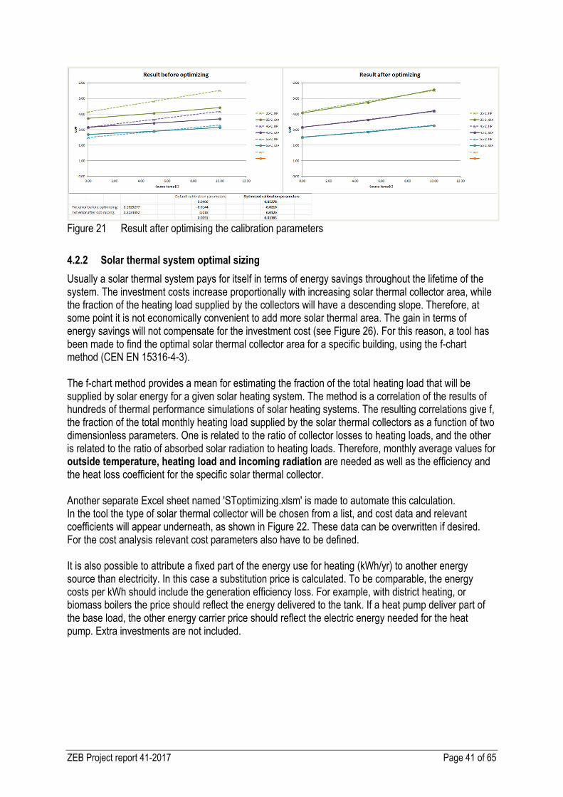
ZEB Project report 41-2017 Page 41 of 65
Figure 21 Result after optimising the calibration parameters
4.2.2 Solar thermal system optimal sizing
Usually a solar thermal system pays for itself in terms of energy savings throughout the lifetime of the system. The investment costs increase proportionally with increasing solar thermal collector area, while the fraction of the heating load supplied by the collectors will have a descending slope. Therefore, at some point it is not economically convenient to add more solar thermal area. The gain in terms of energy savings will not compensate for the investment cost (see Figure 26). For this reason, a tool has been made to find the optimal solar thermal collector area for a specific building, using the f-chart method (CEN EN 15316-4-3). The f-chart method provides a mean for estimating the fraction of the total heating load that will be supplied by solar energy for a given solar heating system. The method is a correlation of the results of hundreds of thermal performance simulations of solar heating systems. The resulting correlations give f, the fraction of the total monthly heating load supplied by the solar thermal collectors as a function of two dimensionless parameters. One is related to the ratio of collector losses to heating loads, and the other is related to the ratio of absorbed solar radiation to heating loads. Therefore, monthly average values for outside temperature, heating load and incoming radiation are needed as well as the efficiency and the heat loss coefficient for the specific solar thermal collector. Another separate Excel sheet named 'SToptimizing.xlsm' is made to automate this calculation. In the tool the type of solar thermal collector will be chosen from a list, and cost data and relevant coefficients will appear underneath, as shown in Figure 22. These data can be overwritten if desired. For the cost analysis relevant cost parameters also have to be defined. It is also possible to attribute a fixed part of the energy use for heating (kWh/yr) to another energy source than electricity. In this case a substitution price is calculated. To be comparable, the energy costs per kWh should include the generation efficiency loss. For example, with district heating, or biomass boilers the price should reflect the energy delivered to the tank. If a heat pump deliver part of the base load, the other energy carrier price should reflect the electric energy needed for the heat pump. Extra investments are not included.

ZEB Project report 41-2017 Page 42 of 65
Figure 22 Input for the ST optimising tool
| The following section describe the steps to get monthly average data from IDA-ICE for outside temperature, heating load and incoming radiation. Three different tables must be copy-pasted into the excel-tool as given in Figure25. 1) The climate table can be obtained directly by opening the climate file in IDA-ICE and press “view data”.
2) The total heating and cooling table requires that an annual simulation is performed, and the table will then be available in the results tab of IDA-ICE.
3) The incoming radiation (W/m2 collector area), will be available in a simulation result table after an annual simulation is completed with a solar thermal system in ESBO.
It is important to note that the incoming radiation is per square meters of collector area, i.e. different tilting angles will give different data. Therefore, if considering different tilting angles, new simulations must be performed to get the correct data. For simplicity one can do the simulation with only one square meter of ST, since the data in the table always will be given as incoming radiation per area.
Figure 23 Input tables for the ST optimising tool
After a calculation is performed in Excel the results will be presented as a list with the solar fraction and the total savings for a range of different collector area. The tool will also print a graph (Figure 26). In the figure the red line represents the solar fraction for a given collector area, while the blue line represents the total savings for that area. The optimal area and the corresponding savings, and the solar fraction are printed in the list to the right.
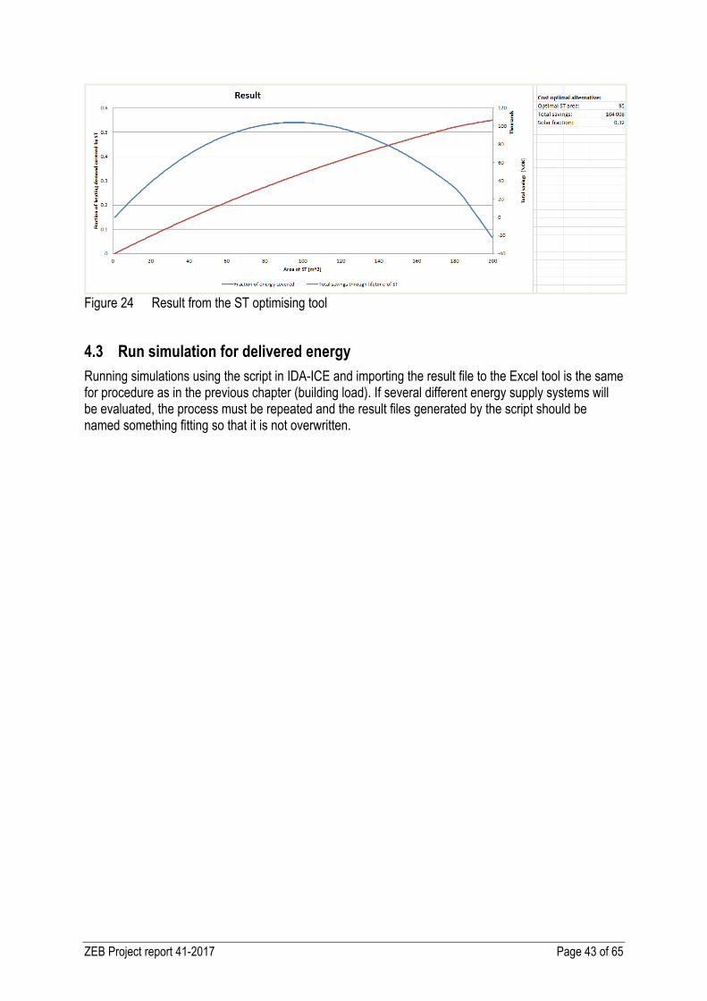
ZEB Project report 41-2017 Page 43 of 65
Figure 24 Result from the ST optimising tool
4.3 Run simulation for delivered energy
Running simulations using the script in IDA-ICE and importing the result file to the Excel tool is the same for procedure as in the previous chapter (building load). If several different energy supply systems will be evaluated, the process must be repeated and the result files generated by the script should be named something fitting so that it is not overwritten.
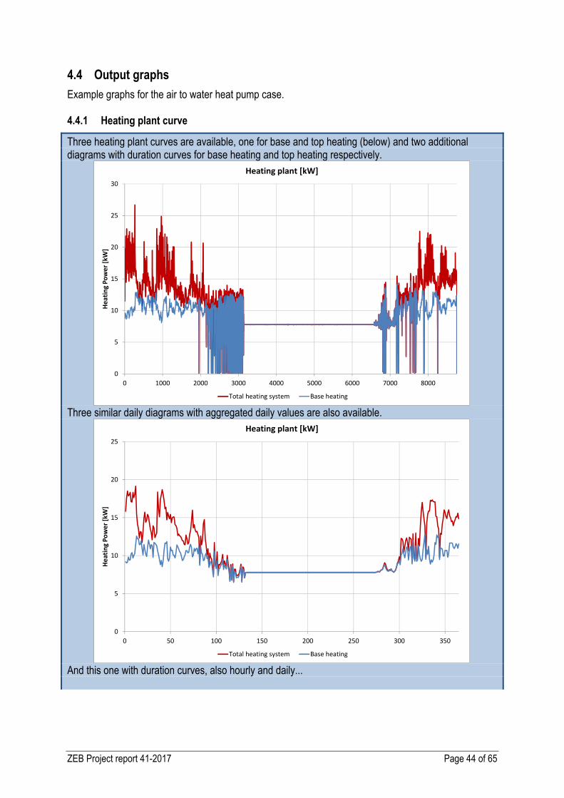
ZEB Project report 41-2017 Page 44 of 65
4.4 Output graphs
Example graphs for the air to water heat pump case. 4.4.1 Heating plant curve
Three heating plant curves are available, one for base and top heating (below) and two additional diagrams with duration curves for base heating and top heating respectively.
Three similar daily diagrams with aggregated daily values are also available.
And this one with duration curves, also hourly and daily...
0
5
10
15
20
25
30
0 1000 2000 3000 4000 5000 6000 7000 8000
Heat
ing
Pow
er [k
W]
Heating plant [kW]
Total heating system Base heating
0
5
10
15
20
25
0 50 100 150 200 250 300 350
Heat
ing
Pow
er [k
W]
Heating plant [kW]
Total heating system Base heating
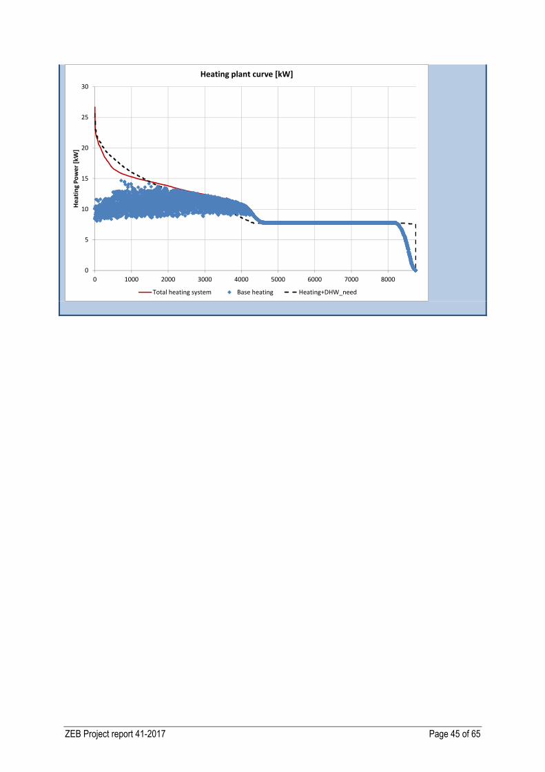
ZEB Project report 41-2017 Page 45 of 65
0
5
10
15
20
25
30
0 1000 2000 3000 4000 5000 6000 7000 8000
Heat
ing
Pow
er [k
W]
Heating plant curve [kW]
Total heating system Base heating Heating+DHW_need
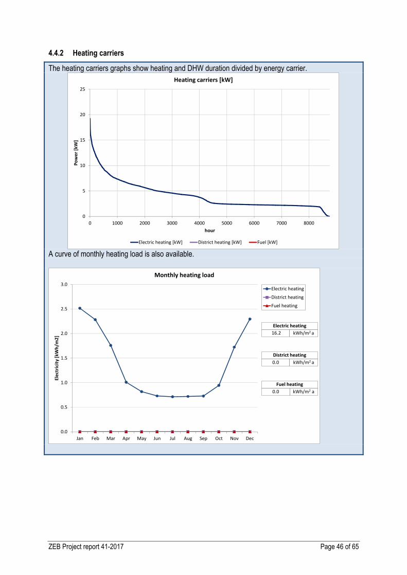
ZEB Project report 41-2017 Page 46 of 65
4.4.2 Heating carriers
The heating carriers graphs show heating and DHW duration divided by energy carrier.
A curve of monthly heating load is also available.
0
5
10
15
20
25
0 1000 2000 3000 4000 5000 6000 7000 8000
Pow
er [k
W]
hour
Heating carriers [kW]
Electric heating [kW] District heating [kW] Fuel [kW]
0.0
0.5
1.0
1.5
2.0
2.5
3.0
Jan Feb Mar Apr May Jun Jul Aug Sep Oct Nov Dec
Elec
tric
ity [k
Wh/
m2]
Monthly heating load
Electric heating
District heating
Fuel heating
Electric heatingkWh/m2 a16.2
District heating0.0 kWh/m2 a
0.0 Fuel heating
kWh/m2 a

ZEB Project report 41-2017 Page 47 of 65
4.4.3 Heat pump details
Heat pump compressor power and COP performance is sorted by the total heating system duration curve below.
The heat pump operating temperatures are sorted by COP in another diagram.
0.0
1.0
2.0
3.0
4.0
5.0
6.0
7.0
0
5
10
15
20
25
30
0 1000 2000 3000 4000 5000 6000 7000 8000
COP
[-]
Pow
er [k
W]
Heat Pump: Compressor Power and COP
Total heating system Compressor power COP
-30
-20
-10
0
10
20
30
40
50
60
70
0.0
1.0
2.0
3.0
4.0
5.0
6.0
7.0
0 1000 2000 3000 4000 5000 6000 7000 8000
Tem
pera
ture
[C]
COP
[-]
Heat Pump: Temperatures sorted by COP
COP Condensation T Evaporation T
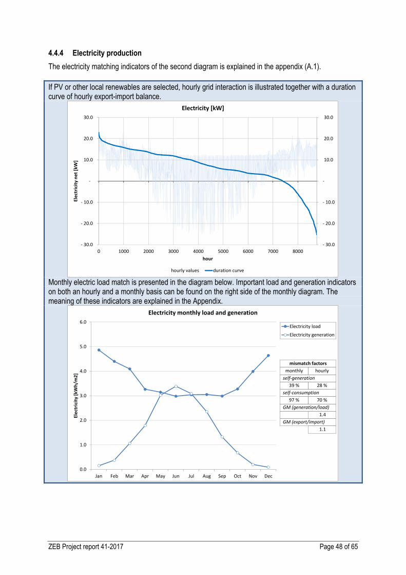
ZEB Project report 41-2017 Page 48 of 65
4.4.4 Electricity production
The electricity matching indicators of the second diagram is explained in the appendix (A.1). If PV or other local renewables are selected, hourly grid interaction is illustrated together with a duration curve of hourly export-import balance.
Monthly electric load match is presented in the diagram below. Important load and generation indicators on both an hourly and a monthly basis can be found on the right side of the monthly diagram. The meaning of these indicators are explained in the Appendix.
- 30.0
- 20.0
- 10.0
-
10.0
20.0
30.0
- 30.0
- 20.0
- 10.0
-
10.0
20.0
30.0
0 1000 2000 3000 4000 5000 6000 7000 8000
Elec
tric
ity n
et [k
W]
hour
Electricity [kW]
hourly values duration curve
0.0
1.0
2.0
3.0
4.0
5.0
6.0
Jan Feb Mar Apr May Jun Jul Aug Sep Oct Nov Dec
Elec
tric
ity [k
Wh/
m2]
Electricity monthly load and generation
Electricity load
Electricity generation
mismatch factorsmonthly hourly
self-generation39 % 28 %
self-consumption97 % 70 %
GM (generation/load)1.4
GM (export/import)1.1
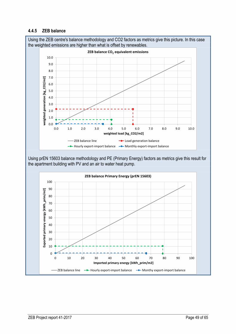
ZEB Project report 41-2017 Page 49 of 65
4.4.5 ZEB balance
Using the ZEB centre's balance methodology and CO2 factors as metrics give this picture. In this case the weighted emissions are higher than what is offset by renewables.
Using prEN 15603 balance methodology and PE (Primary Energy) factors as metrics give this result for the apartment building with PV and an air to water heat pump.
0.0
1.0
2.0
3.0
4.0
5.0
6.0
7.0
8.0
9.0
10.0
0.0 1.0 2.0 3.0 4.0 5.0 6.0 7.0 8.0 9.0 10.0
wei
ghte
d ge
nera
tion
[kg_
CO2/
m2]
weighted load [kg_CO2/m2]
ZEB balance CO2 equivalent emissions
ZEB balance line Load generation balanceHourly export-import balance Monthly export-import balance
0
10
20
30
40
50
60
70
80
90
100
0 10 20 30 40 50 60 70 80 90 100
Expo
rted
prim
ary
ener
gy [k
Wh_
prim
/m2]
Imported primary energy [kWh_prim/m2]
ZEB balance Primary Energy (prEN 15603)
ZEB balance line Hourly export-import balance Monthy export-import balance
ZEB Project report 41-2017 Page 50 of 65
5. Cost Optimality
The European cost-optimal methodology makes it possible to compare and choose between different energy supply solutions, for example a bio stove or a heat pump, or other energy measures, even though they may have different annual costs, different lifetimes, consume different fuels, etc. “The European cost-optimal methodology specifies how to compare energy efficiency measures, measures incorporating renewable energy resources and packages of such measures in relation to their energy performance and the cost attributed to their implementation and how to apply these to selected energy reference buildings with the aim of identifying cost-optimal levels of minimum energy performance requirements” (European Commission, 2012) This is possible by converting all costs attributed to their implementation into global costs, and their energy consumption into primary energy consumption. This is described in detail further in appendices. It should be pointed out that the tool aims at calculating the cost-optimal energy supply solutions and other energy measures, given some minimum energy performance requirements, for any buildings at an early construction phase instead of being limited to one or few reference buildings.
5.1 Calculation of global costs
5.1.1 Product Database11
To easily be able to do a cost analysis, a product database with all the necessary information as given in the cost-optimal methodology should be available. As for now the database contains cost data and performance data for the following energy systems: Solar thermal collectors (ST), Photovoltaic (PV), Bio boilers (Bio), Air to Water Heat Pumps (AWHP), Ground Source Heat Pumps (GSHP), District Heating (DH), Combined Heat and Power (CHP). The amount of data for each energy system varies, but it is certain that the database should be updated and expanded for more accurate future cost analyses. Most of the cost data in the database have been obtained by producers. Some data have also been obtained by contacting ZEB industrial partners in order to get existing data from earlier projects. 5.1.2 Cost analysis tool
To easily be able to utilise the database for early stage cost analyses, a simple tool was made in some of the ZEB tool Excel sheets, see Figure 27, containing cost data for all the products in the database. The user will set input parameters like appropriate rates (energy price escalation rate, inflation, discount rate), energy prices, calculation period, and choose the amount of imported and exported energy (obtained from the simulation in IDA-ICE). The user must also choose the energy supply system by marking out the different technologies and selecting between different products in a list. For ST and PV it is also important to select the total area used. It is also possible to choose an alternative called “customise” where the users can insert their own data. When everything is set, calculation button is pressed and the program will calculate the total global costs for the chosen calculation period, i.e. total energy costs, investment costs, annual costs, replacement costs and residual values. The tool will also calculate the CO2 costs related to the net energy use in the building. CO2 emission related to production of materials and products is not taken into consideration.
11 In 2012 a project work was carried out by Sjur Vullum Løtveit at the Norwegian University of Science and Technology (Løtveit, 2012) to start developing such a database.
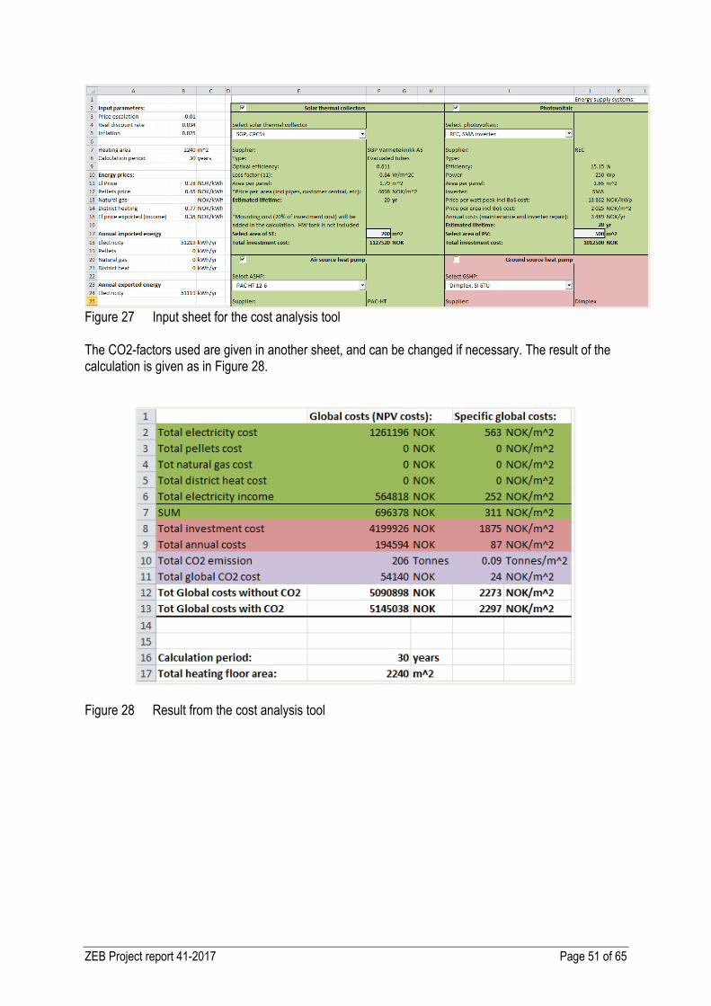
ZEB Project report 41-2017 Page 51 of 65
Figure 27 Input sheet for the cost analysis tool The CO2-factors used are given in another sheet, and can be changed if necessary. The result of the calculation is given as in Figure 28.
Figure 28 Result from the cost analysis tool
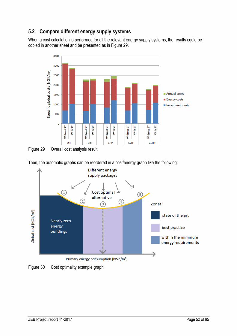
ZEB Project report 41-2017 Page 52 of 65
5.2 Compare different energy supply systems
When a cost calculation is performed for all the relevant energy supply systems, the results could be copied in another sheet and be presented as in Figure 29.
Figure 29 Overall cost analysis result
Then, the automatic graphs can be reordered in a cost/energy graph like the following:
Figure 30 Cost optimality example graph
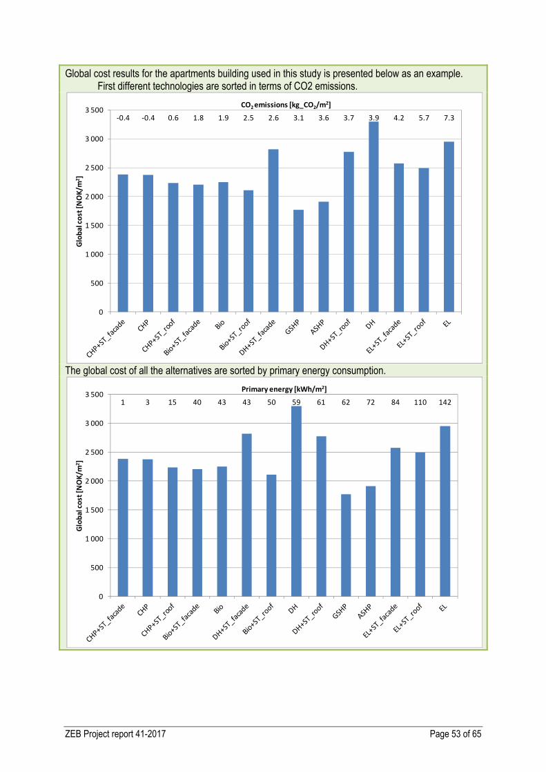
ZEB Project report 41-2017 Page 53 of 65
Global cost results for the apartments building used in this study is presented below as an example. First different technologies are sorted in terms of CO2 emissions.
The global cost of all the alternatives are sorted by primary energy consumption.
-0.4 -0.4 0.6 1.8 1.9 2.5 2.6 3.1 3.6 3.7 3.9 4.2 5.7 7.3
-1.00
0.00
1.00
2.00
3.00
4.00
5.00
6.00
7.00
8.00
0
500
1 000
1 500
2 000
2 500
3 000
3 500CO2 emissions [kg_CO2/m2]
Glob
al co
st [N
OK/
m2 ]
1 3 15 40 43 43 50 59 61 62 72 84 110 142
0.00
20.00
40.00
60.00
80.00
100.00
120.00
140.00
160.00
0
500
1 000
1 500
2 000
2 500
3 000
3 500Primary energy [kWh/m2]
Glob
al co
st [N
OK/
m2 ]
ZEB Project report 41-2017 Page 54 of 65
6. Discussion and Conclusions
6.1 Discussion
Experience from the pilot projects of the ZEB centre revealed the need for more knowledge and better supporting tools for the analysis and choice of energy systems in the early design phase. Since no universally recognised ZEB definition exists, it is important to evaluate different metrics, e.g. primary energy and carbon emissions. Awaiting for new international standards to be devised and enter into force (e.g. ISO 52000-1 / EN 15603) it was also important to recognise that different types of balance are possible, such as a load-generation balance and an import-export balance (Sartori et al., 2012). Furthermore, several indicators may be considered to describe the mismatch between load and generation as well as the interaction of ZEBs with the grids (Salom et al., 2014). Lastly, the choice between alternative solutions for the energy system should be based on principles of cost optimality (Cost-optimal methodology and accompanying technical guidelines, EU 244/2012). General feedback on the tool: In October 2015, a near-final version of the ZEB tool was sent to selected internal and external evaluators (researchers and practitioners in the industry respectively). The task was to try to simulate 2-3 alternative designs. Included in the guidelines were a building model sample of an apartment building, the ZEB tool, and additional Excel files. Feedback on the usability and application of the ZEB tool was positive among evaluators. Leading up to the evaluation, the internal review process and development had been going on for a long time. The outcome is a script for IDA that handles all the parameters of interest from a whole-year simulation run, and the post-processing of this data in Excel (in what is called the ZEB tool). From the time this work was started, the ESBO plant has become a more mature tool. The default control strategy of the plant performs better, and some modules have more parameters than initially. For example, improvements have been made to control the solar thermal collector loop, and it works better than before in combination with heat pumps. Other changes are more possibilities to set temperature limits and other boundary conditions within the heat pump models. The ZEB tool can be somewhat demanding for the early design phase. It was noted by one group of reviewers that setting up the model and running the simulation take a long time, making it difficult to use in a workshop context where one quickly wants to compare different possibilities. It is true that it will be difficult to use the ZEB tool ad-hoc in a workshop the same way that many are used to with Excel tools. Preparing a building model in IDA and verifying the simulations is necessary in order to use the tool, but when the model is completed it is relatively easy to simulate more design alternatives. In the current form, the ZEB tool only loads results from one simulation at the time. To compare different energy plants or design alternatives, multiple Excel files are needed, which can be time-consuming. A separate Excel tool was made to load and sort results from multiple simulations, enabling comparisons of performance over a longer calculation period (chapter 6). Since Excel is flexible to use, simulators may prefer to make their own diagrams and tables for comparison. In a workshop setting, simple calculation tools i.e. focusing on monthly energy production and demand profiles will be a faster approach to providing quick answers. Some reviewers suggested that templates should be made to work with other BPS software and less dynamic evaluation tools such as SIMIEN and TEK-SJEKK. Indeed, it would be possible to create result templates with ZEB-metrics and diagrams for simple calculation tools like SIMIEN and TEK-SJEKK, but evidently, results cannot be represented in more detail than the underlining model. There are many important aspects of ZEB energy design that require a dynamic model to be evaluated properly, i.e. plant temperature levels, combinations of energy systems, availability of renewable or ambient heat sources over course of the year, detailed sub-system efficiencies, part load and energy cover factors (to mention some central energy design problems). As
ZEB Project report 41-2017 Page 55 of 65
for the building load model different scenarios of occupancy and more dynamic user load patterns can be evaluated with a detailed calculation model. How detailed should the model be? – is an important question when working with advanced BPS tools like IDA-ICE. The total simulation time, including the calculation time and the time it takes to model, largely depend on the complexity of the building model and the energy supply. It is a relationship with diminishing returns, meaning that achieving greater levels of accuracy may become very time-consuming. Therefore, it is important to find a sufficient detail level for the early phase. In practice, this typically includes combining thermal zones, simplifying geometry and merging window units within the building model. As a rule of thumb, the dynamic exchange of different systems (or components), i.e. building load and energy supply system, should be modelled in greatest detail were the two systems greatly impact each others performance. On the other hand, taking the time to model two systems that barely interact is of little use. A good principle is to focus on the aspects the designer has the most influence over at the early design stage, prioritising decisions with considerable impact on the energy performance. The ZEB tool can be used to show the design team which decisions are critical to reaching ZEB ambitions, through balancing low energy demand with on-site energy production and evaluating cost-effective energy system solutions over the economic life. Suggestions for future work Several testers requested an annual energy budget to get an overview of energy for lighting, electric equipment as well as heating and HVAC purposes. An energy demand budget such as in NS 3031 will not be straightforward to implement based on the result file from IDA. With the new technical supplement SN/TS 3031:2016 an alternative to the standard calculation scheme of "netto energibehov" is proposed. With the parameters in the result file generated from IDA-ICE it would be possible to the create nearly all the tables in SN/TS 3031:2016 (result table 4-8, except table 5 which is distribution and storage losses). In a future
Some additional suggestions for improving the tool Building load: A diagram showing outdoor temperature overlaid to building load on a time series diagram (hourly, or daily
values for a whole year), optionally with the temperature scale inverted to see the correlation to energy demand. This type of diagram is common in energy management software portals.
X-axis that shows the date, or month as well as hour 0-8760.
Energy supply: Include percentage load cover and energy cover factors in the heating plant diagrams. More graphs showing the energy generation and import/export on an hourly basis, i.e. time series charts
and carpet plots to understand how it varies in time over the year. A simple method to evaluate battery storage from post-processing the results in Excel. Costs: Greater transparency in terms of cost assumptions. Most important for developers and entrepreneurs, and
what consultants will be held responsible for in the next phase. What is included, what cost is defined for different components and parts of the system etc.
Energy costs, and electricity price in particular, is difficult to relate to in a simple economic analysis. In reality, large customers will often have a tariff based on maximum demand or a power factor of the customers' load. Instead of a flat rate (which is currently used in the economic evaluation), there could also be a part tariff scheme divided between fixed costs, semi-fixed costs and running costs. With hourly results from IDA-ICE there is a possibility to calculate energy cost based on a more advanced tariff, but since each supply/utility company has chosen a different scheme to charge for electricity use, it would be difficult to implement a general model.
ZEB Project report 41-2017 Page 56 of 65
6.2 Conclusion
The need for more knowledge and better supporting tools for the choice of energy systems for ZEBs is evident within the pilot projects of the Norwegian ZEB centre. Internationally, it is also recognised that tools must become more effective and informative in order to support ZEB design decisions. An international survey among practitioners of building performance simulations (BPS) found that they need fluid tools to produce initial results from rough representations during early stage and at the same time allow for detailing of components during later phases (Attia, 2011). The IDA Early Stage Building Optimization plant (ESBO plant) enables comparison of different energy supply systems by still keeping to a bare minimum of input data from the user (EQUA, 2015). With the ESBO plant it is possible to simulate dynamic exploitation of energy flows and integration between heating and cooling plant, building load and other ambient heat sinks or sources. ESBO enable performance evaluation over the influence of temperature levels, component size dimensioning, and other energy design parameters typically otherwise selected based on rules of thumbs and basic analysis. The concept of the IDA ESBO plant model fit well with the aim to evaluate different energy systems for ZEBs, and the plant model can also be used further in design detailing. Sartori et.al. (2012) identifies several metrics (based on energy, emissions and economical balance concepts) that are important to evaluate. The assessment also recognises that different definitions of zero emission, or zero energy buildings are possible. Load-generation match, as well as import and export type of balances can be calculated from simulations. The support tool developed in Excel offers to automate this process. A scripted simulation run from within IDA-ICE generates a result file which is loaded into the templates. The result file has one value for each hour of the year with columns of hourly aggregated building load, plant temperatures, mass flows and energy exchange between components. Depending on the energy supply system, the parameters to be accounted for are calculated in the tool and presented through a series of diagrams. BPS tools have different analysis and reporting capabilities, but as the study by Attia found, most tools has poor integration of ZEB metrics from within the software. Furthermore, BPS tools traditionally addressed the later design stages. In order to provide feedback to the design team, results must communicate not only by the usual aggregated predicted building performance data (e.g., total annual energy consumption), but provide insights into the choices that the designers has influence over. A well presented case may allow "what if" questions to be answered and engage not only the experts, but other stakeholders too. Therefore, the result templates has many type of diagrams and comparison tables. Specific diagrams are also available for heat pumps, or if other energy carriers than electricity is used for heating. Primary energy, or emission factors can be adjusted within the spreadsheet application, as well as energy costs and other costs related to an economic evaluation following the European cost-optimal methodology. In a design process, there is always limited time, and a lack of time and resources to verify simulations. The templates are currently undergoing evolution among Norwegian building designers. So there is a need for easy to use tools that can help to take decisions on the basis of very limited knowledge. We hope that the templates will receive positive feedback and be put to use at the early design stage of projects that are evaluating ZEB ambitions. When methods and defintitions have matured, there will be more efforts to include ZEB evaluation criteria in existing tools. In the meantime, using Excel is a robust and transparent method to present data from simulations and allow for easy modifications.

ZEB Project report 41-2017 Page 57 of 65
7. References
Attia, S., Beltran, L., De Herde, A. and Hensen J. (2009) Architectfriendly: a comparison of ten different building performance simulation tools. In Proceedings of IBPSA 2009 Buildings Simulation Conference, p. 204–211, 2009.
Attia S and De Herde A, (2011a) Early design simulation tools for net zero energy buildings: a comparison of ten tools, International building performance simulation association, November 2011, Sydney, Australia
Attia, S. and La Neuve, L. (2010) Building performance simulation tools: selection criteria and user survey. Louvain Catholic University, Louvain-la-Neuve.
Attia S, et al., (2011b) Selection criteria for building performance simulation tools: contrasting architects' and engineers' needs', Journal of building performance simulation, First published on: 12 April 2011.
Attia S, (2012a) Optimisation for Zero Energy Building Design: Interviews with Twenty Eight International Experts, Architecture et Climat, Louvain La Neuve: Université catholique de Louvain,
Attia, S., Gratia, E. et al. (2012b) Simulation-based decision support tool for early stages of zero-energy building design. Energy and Buildings 49(0): 2-15.
Baranda, P. B. (2014) Cost optimality of Energy Systems in Zero Emission Buildings in Early Design Phase, Master's Thesis, Department of Energy and Process Engineering: Norwegian University of Science and Technology.
Bamford, G. (2002) From analysis / synthesis to conjecture / analysis: a review of karl popper’s influence on design methodology in architecture. Design Studies, 23(3):245–261.
Crawley, D.B., Hand, J.W., Kummert, M., and Griffith, B.T. (2008) Contrasting the capabilities of building energy performance simulation programs. Journal of Building and Environment 43(4): 661-673.
Eriksson, J., Systemmodell för dimensionering och optimering av energicentral med borrhålslager. 2010, ÅFORSK – Ångpanneföreningens Forskningsstiftelse. p. 44.; Available from: [link]
European Commission, EU cost-optimal methodology, guidelines. Office Journal of the European Union, 2012: [p. 19., p. 28.]
European Parliament and the Council (2010). Directive 2010/31/EU of The European Parliament and the Council of 19 May 2010 on the Energy Performance of Buildings. The european parliament and the council of the european union. Directive, 2010/31/EU
EQUA (2015) IDA Early Stage Building Optimization (ESBO) – User guide. Document version 2.0, May 2015. Copyright 2012 - 2015 EQUA Simulation AB.
EQUA (2016) User Manual – IDA Indoor Climate and Energy Version 4.7. EQUA Simulation AB January 2016. Copyright © 2009-2016 EQUA Simulation AB.
Hass, J., Weir, M.D., and Thomas, G.B., Calculus Part 1. 2008: Pearson.p. 516-518
Loukissas, Y.A. (2012) Co-Designers: Cultures of Computer Simulation in Architecture. Taylor and Francis.
Løtveit, S.V. (2012) Information database for supply in decision making on ZEB energy system in early design stage, Department of Physics: Norwegian University of Science and Technology. p. 60.
Løtveit, S.V. (2013) Cost optimality of Energy Systems in Zero Emission Buildings in Early Design Phase, Master of Science in Physics and Mathematics, Department of Physics: Norwegian University of Science and Technology.
ZEB Project report 41-2017 Page 58 of 65
Noris, F., Musall, E., Salom, J., B. Berggren, B., Østergaard Jensen, S., Lindberg K., Sartori, I. (2014) Implications of weighting factors on technology preference in net zero energy buildings. Energy and Buildings 82: 250-262.
O’Brien W.L. (2012) Preliminary investigation of the use of sankey diagrams to enhance building performance simulation supported design. In L Nikolovska and R Attar, editors, Symposium on Simulation for Architecture and Urban Design, 2012.
Salom, J., Marszal, A., Candanedo, J., Widen, J., Lindberg, K., Sartori I. (2014). "Analysis of load match and grid interaction indicators in net zero energy buildings with simulated and monitored data." Applied Energy 136: 119-131.
Salom, J., Marszal, A., Candanedo, J., Widen, J., Lindberg, K., Sartori, I. (2012) Analysis of load match and grid interaction indicators in net zero energy buildings with high-resolution data. Report available for download at http://task40.iea-shc.org/publications.
Sartori, I., Napolitano, A., Voss, K. (2012) Net zero energy buildings: A consistent definition framework. Energy and Buildings 48: 220-232.
Sartori, I., Ortiz, J., Salom, J., Dar, U.I. (2014) Estimation of load and generation peaks in residential neighbourhoods with BIPV: bottom-up simulations vs. Velander. World Sustainable Building Conference 2014, Barcelona.
Sartori, I., Merlet, S., Thorud, B., Haug, B., Andresen, I. (2016) Zero Village Bergen – Aggregated loads and PV generation profiles. ZEB Report.
Sartori, I., Skeie, K.S., Sørnes, K., Andresen, I. (2017) Zero Village Bergen – Energy system analysis. ZEB Report.
Standard Norge, NS 3031: Beregninger av bygningers energiytelse, Metode og data. 2014. p. 74.
Standard Norge, NS-EN 14511-2:2013: Klimaaggregater, væskekjøreaggregater og varmepumper med elektrisk drevne kompressorer for oppvarming og avkjøling av rom, Del 2-prøvingsbetingelser. 2013. p. 19.
The European Committee for Standardization (CEN), NS-EN 15459: Bygningers energiytelse. Økonomisk evalueringsprosedyre for energisystemer i bygninger. 2007. p. 50.
Trebilcock, M. (2009) Integrated design process: From analysis/synthesis to conjecture/analysis. In PLEA 2009 Conference proceedings.

ZEB Project report 41-2017 Page 59 of 65
Appendices

ZEB Project report 41-2017 Page 60 of 65
A1. Electricity match indicators
Figure shows a generic monthly electric load and PV generation profile with the purpose of visualising the areas A, B and C used in the equations of the mismatch factors as calculated on a monthly and hourly basis in the ZEB tool. The shape of the curves would be different for buildings using CHP, or wind generation or located in cooling dominated climates. In terms of net monthly values, area A represents electricity export to the grid while area B represents electricity delivered by the grid; finally, area C represents the self-covered demand. Hence, A + C is the total electricity generation (Norris et.al. 2014).
Figure 31: Areas for formulas demonstrating monthly electricity load and generation mismatch factors
(Norris et.al. 2014)
Self-generation (demand cover factor) The self-generation (also called load or demand cover factor) represents the percentage of the electrical demand (B+C) covered by on-site electricity generation and is defined as = = ∑ [ ( ), ( )]∑ ( ) [%] 1
where: lel(t) electricity load (kW). gel(t) on-site electricity generation (kW). t is the evaluation period, in this case the net values of 12 months. For hourly mismatch, the number of samples are 8760 for the entire year. Self-consumption (supply cover factor) The self-consumption (also called supply cover factor) indicate the fraction of on-site electricity generation (A + C) being self-consumed (C) by the building (within the resolution time step). = = ∑ [ ( ), ( )]∑ ( ) [%] 2
Other versions of the equations for grid interaction indexes can be found in literature. The mismatch factors of the ZEB tool only consider electricity, but there are also more detailed demand and supply cover factors that includes other energy carriers and that account for battery storage in the following reports (Salom et. al. 2012) (Salom et. al. 2014).
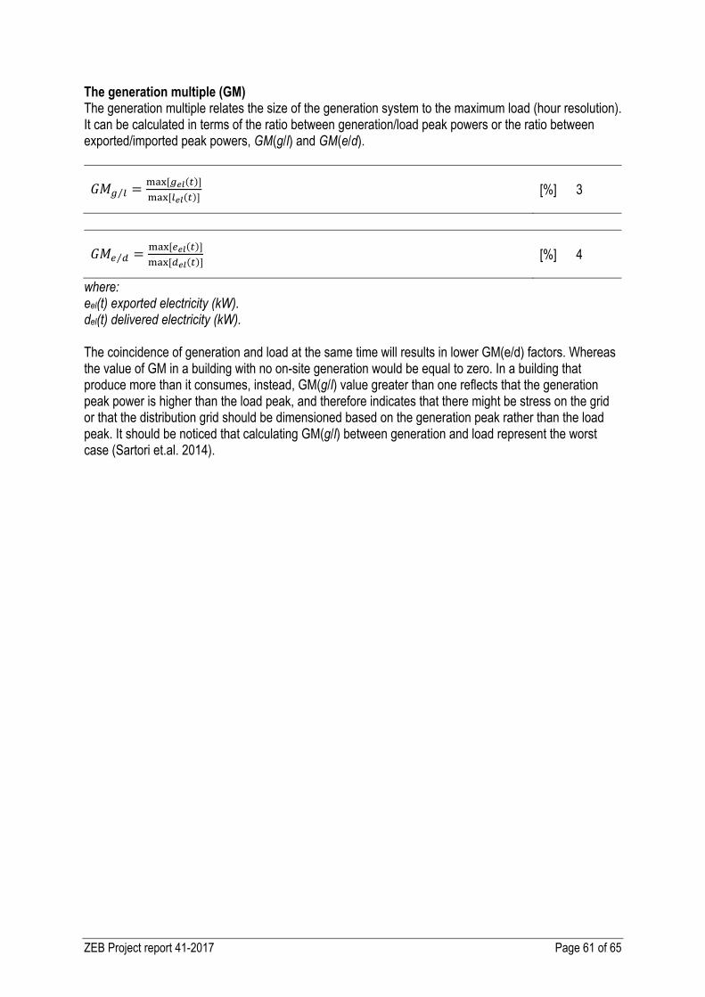
ZEB Project report 41-2017 Page 61 of 65
The generation multiple (GM) The generation multiple relates the size of the generation system to the maximum load (hour resolution). It can be calculated in terms of the ratio between generation/load peak powers or the ratio between exported/imported peak powers, GM(g/l) and GM(e/d).
⁄ = [ ( )][ ( )] [%] 3
⁄ = [ ( )][ ( )] [%] 4
where: eel(t) exported electricity (kW). del(t) delivered electricity (kW). The coincidence of generation and load at the same time will results in lower GM(e/d) factors. Whereas the value of GM in a building with no on-site generation would be equal to zero. In a building that produce more than it consumes, instead, GM(g/l) value greater than one reflects that the generation peak power is higher than the load peak, and therefore indicates that there might be stress on the grid or that the distribution grid should be dimensioned based on the generation peak rather than the load peak. It should be noticed that calculating GM(g/l) between generation and load represent the worst case (Sartori et.al. 2014).
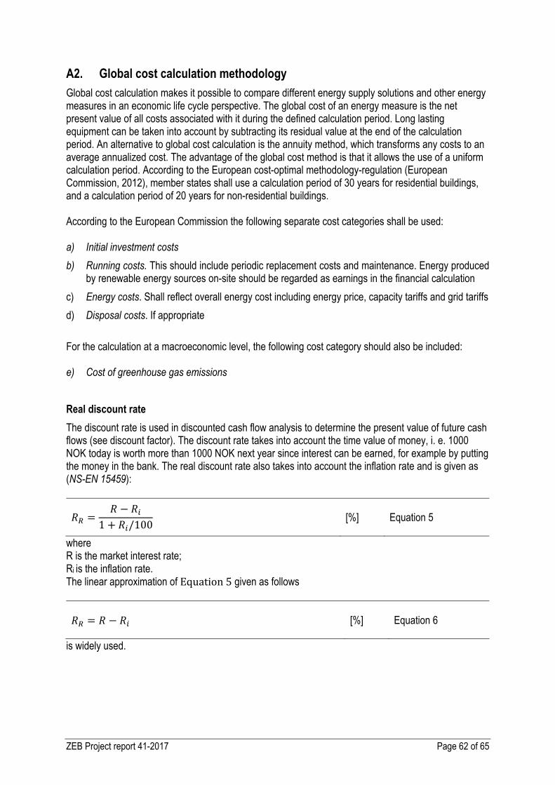
ZEB Project report 41-2017 Page 62 of 65
A2. Global cost calculation methodology
Global cost calculation makes it possible to compare different energy supply solutions and other energy measures in an economic life cycle perspective. The global cost of an energy measure is the net present value of all costs associated with it during the defined calculation period. Long lasting equipment can be taken into account by subtracting its residual value at the end of the calculation period. An alternative to global cost calculation is the annuity method, which transforms any costs to an average annualized cost. The advantage of the global cost method is that it allows the use of a uniform calculation period. According to the European cost-optimal methodology-regulation (European Commission, 2012), member states shall use a calculation period of 30 years for residential buildings, and a calculation period of 20 years for non-residential buildings. According to the European Commission the following separate cost categories shall be used: a) Initial investment costs
b) Running costs. This should include periodic replacement costs and maintenance. Energy produced by renewable energy sources on-site should be regarded as earnings in the financial calculation
c) Energy costs. Shall reflect overall energy cost including energy price, capacity tariffs and grid tariffs
d) Disposal costs. If appropriate
For the calculation at a macroeconomic level, the following cost category should also be included: e) Cost of greenhouse gas emissions
Real discount rate
The discount rate is used in discounted cash flow analysis to determine the present value of future cash flows (see discount factor). The discount rate takes into account the time value of money, i. e. 1000 NOK today is worth more than 1000 NOK next year since interest can be earned, for example by putting the money in the bank. The real discount rate also takes into account the inflation rate and is given as (NS-EN 15459):
where R is the market interest rate; Ri is the inflation rate. The linear approximation of Equation5 given as follows
is widely used.
= −1 + /100 [%] Equation 5
= − [%] Equation 6
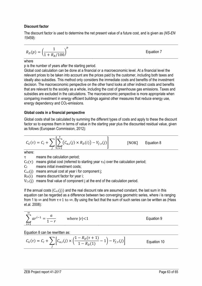
ZEB Project report 41-2017 Page 63 of 65
Discount factor
The discount factor is used to determine the net present value of a future cost, and is given as (NS-EN 15459): ( ) = 11 + /100 Equation 7
where p is the number of years after the starting period. Global cost calculation can be done at a financial or a macroeconomic level. At a financial level the relevant prices to be taken into account are the prices paid by the customer, including both taxes and ideally also subsidies. This method only considers the immediate costs and benefits of the investment decision. The macroeconomic perspective on the other hand looks at other indirect costs and benefits that are relevant to the society as a whole, including the cost of greenhouse gas emissions. Taxes and subsidies are excluded in the calculations. The macroeconomic perspective is more appropriate when comparing investment in energy efficient buildings against other measures that reduce energy use, energy dependency and CO2-emissions. Global costs in a financial perspective
Global costs shall be calculated by summing the different types of costs and apply to these the discount factor so to express them in terms of value in the starting year plus the discounted residual value, given as follows (European Commission, 2012): ( ) = + , ( ) × ( ) − , ( ) [NOK] Equation 8
where: τ means the calculation period; CG(τ) means global cost (referred to starting year τ0) over the calculation period; CI means initial investment costs; Ca,i(j) means annual cost at year i for component j; RD(i) means discount factor for yeari; Vf,τ(j) means final value of component j at the end of the calculation period. If the annual costs (Ca,i(j))and the real discount rate are assumed constant, the last sum in this equation can be regarded as a difference between two converging geometric series, where i is ranging from 1 to ∞ and from τ+1to∞.By using the fact that the sum of such series can be written as (Hass et.al. 2008): = 1 − where|r|<1 Equation 9
Equation 8 can be rewritten as: ( ) = + , ( ) × 1 − ( + 1)1 − (1) − 1 − , ( ) Equation 10
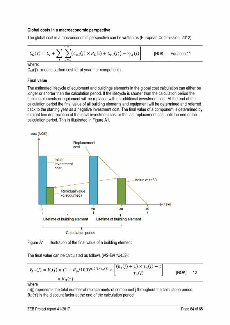
ZEB Project report 41-2017 Page 64 of 65
Global costs in a macroeconomic perspective
The global cost in a macroeconomic perspective can be written as (European Commission, 2012): ( ) = + , ( ) × ( ) + , ( ) − , ( ) [NOK] Equation 11
where: Cc,i(j) means carbon cost for at year i for component j. Final value
The estimated lifecycle of equipment and buildings elements in the global cost calculation can either be longer or shorter than the calculation period. If the lifecycle is shorter than the calculation period the building elements or equipment will be replaced with an additional investment cost. At the end of the calculation period the final value of all building elements and equipment will be determined and referred back to the starting year as a negative investment cost. The final value of a component is determined by straight-line depreciation of the initial investment cost or the last replacement cost until the end of the calculation period. This is illustrated in Figure A1.
Figure A1 Illustration of the final value of a building element
The final value can be calculated as follows (NS-EN 15459):
, ( ) = ( ) × (1 + /100) ( )× ( ) × ( ( ) + 1) × ( ) −( )× ( ) [NOK] 12
where nτ(j)represents the total number of replacements of component j throughout the calculation period; RD(τ)is the discount factor at the end of the calculation period;

ZEB Project report 41-2017 Page 65 of 65
( ) × (1 + /100) ( )× ( ) represents the last replacement cost, when taking into account the price development for the product, Rp (inflation rate is used here); ( ( ) )× ( )( ) is the straight-line depreciation of the last replacement cost.
The Research Centre on Zero emission Buildings (ZEB)The main objective of ZEB is to develop competitive products and solu-tions for existing and new buildings that will lead to market penetration of buildings that have zero emissions of greenhouse gases related to their production, operation and demolition. The Centre will encompass both residential and commercial buildings, as well as public buildings.
Partners
NTNU www.ntnu.no
SINTEF www.sintef.no
Skanska www.skanska.no
Weber www.weber-norge.no
Isola www.isola.no
Glava www.glava.no
Protan www.protan.no
Caverion Norgewww.caverion.no
www.zeb.no
ByBo www.bybo.no
Multiconsult www.multiconsult.no
Brødrene Dahl www.dahl.no
Snøhetta www.snoarc.no
Forsvarsbygg www.forsvarsbygg.no
Statsbygg www.statsbygg.no
Husbanken www.husbanken.no
Byggenæringens Landsforening www.bnl.no
Direktoratet for byggkvalitetwww.dibk.no
DuPontwww.dupont.com
NorDan ASwww.nordan.no
Enovawww.enova.no
SAPA Building system www.sapagroup.com
Sør-Trøndelag fylkeskommunewww.stfk.no
Entra Eiendom ASwww.entra.no