Pacific Lamprey Monitoring

and Data Management

Yakama Nation FRMP

Pacific Lamprey

Recovery Project

3/9/2012

Project Goals

The goal of the Yakama Nation is to restore natural

production of Pacific lamprey to a level that will

provide robust species abundance, significant

ecological contributions and meaningful harvest

throughout the Yakama Nations Ceded Lands and in

the Usual and Accustomed areas.

Pacific Lamprey Adult Counts

Premises

• Yakima population is functionally

extirpated

• Our goal is to have hundreds and

thousands of juveniles

Supplementation a much needed tool

• Genetics (risk management approach)

Monitoring Projects

• Adult passage (radio telemetry)

• Juvenile passage (Prosser Dam) -> index?

• Juvenile present/absence (including canals)

• Juvenile index sites (“relative abundance”)

• Water quality impacts on lamprey (adult/juv.)

• Artificial propagation and rearing (methods, feed)

• Supplementation effectiveness (survival and

growth)

Juvenile Surveys

• Exploratory Survey (Min. Data)

Presence / Absence

Quick survey

• Index Survey (Core Data)

Relative abundance

Annual variation

• Extensive Surveys (Optional Data)

Release from art. prop.

Seasonal variation

Growth, distribution, habitat use

Focus

• Need a method to measure

“relative abundance” of larvae

Time & Space

Consistent

& Coordinated

Precision not important

Density can be misleading

= Type 1

0

0.2

0.4

0.6

0.8

1

1.2

0 50 100Mean Annual Stream Flow (cms)

0

0.2

0.4

0.6

0.8

1

1.2

0 5 10Calibrated Valley Constraint

00.20.40.60.8

11.2

0 5

Channel Gradient (%)

Intrinsic Potential (IP)

Model for Pacific Lamprey

• What is the potential

for lamprey habitat?

• Flow

• Gradient

• Valley Width

• (Temperature)

• Flow

• >14 cfs

• Gradient

• < 2 %

• Valley Width

• > 100 ft

Use Existing Data

ODFW Steelhead Survey

Benefits of IP Model

for Pacific Lamprey

• Higher efficiency in predicting

lower and upper distribution

• Make comparison

of density and

relative abundance

more meaningful

Spatial Scales

• 3 spatial scales

• 10 M: density, habitat

features

• 100 M: relative

abundance, status and trend

• 1000 M: abundance

estimates, status and

trend, limiting factors

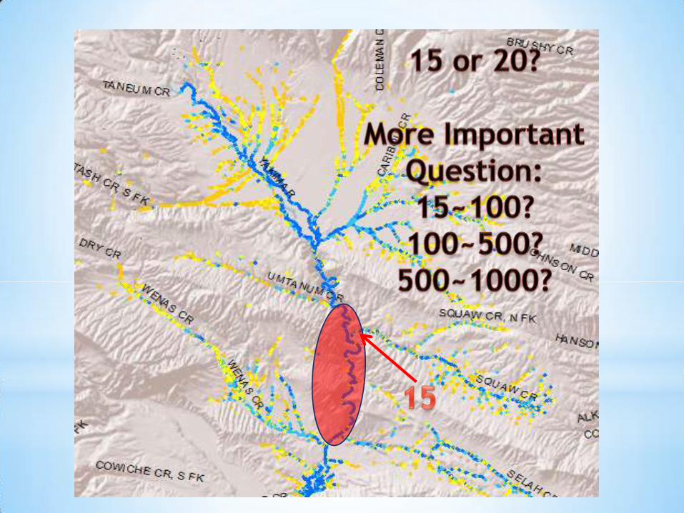
Analysis Unit 2Analysis Unit 1

Analysis Unit 3

LegendIndex Sites

Extensive Sites

Exploratory Sites

Reach A Reach B

Reach D

Reach CReach E

Reach F

Index Sites

density measurements in representative

habitat types -> “relative abundance”

• ~100 meters

• 3-5 plots, fixed and mapped

• Each Plot = X amount of area surveyed over

Y amount of time (~10 m)

• Long-term

Extensive Sitesgrowth, survival and habitat preference

of released propagated larvae.

• ~100 metes

• Extensive area surveyed

• Location may vary over time

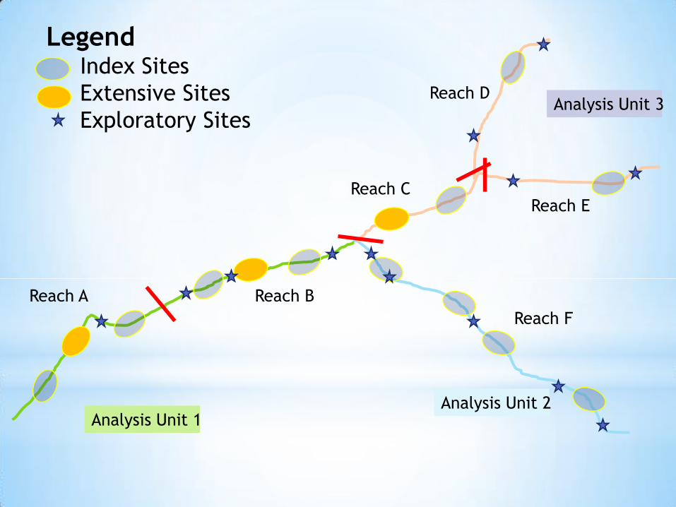
Area

Supplemented

How to Calculate

Abundance??

• Estimate area for Type 1 & 2

Habitat (using habitat surveys)

• Not always available

(Larger streams/rivers)

= 250 m2

Core Data

Reach Scale (~1000 m)

• Watershed (HUC 5 or 6)

• Stream Name

• GPS

• (River Mile -> identifier)

• (Elevation)

• (Gradient)

• (Sinuosity)

Core Data

Habitat Scale (~10 m)

• Channel type (riffle, glide, pool)

• Habitat Type (% Type 1 & 2)

• Plot size

• Method (E-fishing, hand net, etc)

• Survey time (cpue)

• Time of day

• Visibility (high, medium, low)

• (Conductivity)

• (Temperature/DO/pH)

• (Riparian / % cover)

Biological Core Data

• Species (at least %)

• Life stage

• Counts

• (Length)

• (Weight)

Questions??