XMM-Newton Optical and UV Monitor (OM) Calibration...

XMM

XMM-Newton Optical and UV Monitor (OM)Calibration Status

XMM-SOC-CAL-TN-0019 Issue 6.0

Antonio Talavera, OMCal TeamXMM-Newton Science Operations Center

OMCal TeamMSSL-UCL

20 January 2011

Revision history

Revision number Date Revision author Comments

3.2 24 June 2004 B. Chen and OMCal Team last update in old format4.0 25 July 2007 A. Talavera and OMCal Team Reformatted document5.0 30 October 2008 A. Talavera and OMCal Team General update6.0 20 January 2011 A. Talavera and OMCal Team Update

i

european space agencyagence spatiale européenne

XMM Science Operations Team

Document No.: XMM-SOC-CAL-TN-0019Issue/Rev.: 6.0Date: 20 January 2011Page: ii

Contents

1 Introduction 1

2 Instrumental corrections 12.1 Dark count rate . . . . . . . . . . . . . . . . . . . . . . . . . . . . . . . . . . . . . 12.2 Flat fields . . . . . . . . . . . . . . . . . . . . . . . . . . . . . . . . . . . . . . . . 22.3 Bad pixels . . . . . . . . . . . . . . . . . . . . . . . . . . . . . . . . . . . . . . . . 22.4 Operational modes, source detection and count rate . . . . . . . . . . . . . . . . 62.5 Coincidence Loss . . . . . . . . . . . . . . . . . . . . . . . . . . . . . . . . . . . . 62.6 Point Spread Function . . . . . . . . . . . . . . . . . . . . . . . . . . . . . . . . . 72.7 Distortion . . . . . . . . . . . . . . . . . . . . . . . . . . . . . . . . . . . . . . . . 82.8 Large scale Sensitivity variation . . . . . . . . . . . . . . . . . . . . . . . . . . . . 112.9 Background . . . . . . . . . . . . . . . . . . . . . . . . . . . . . . . . . . . . . . . 162.10 Straylight . . . . . . . . . . . . . . . . . . . . . . . . . . . . . . . . . . . . . . . . 172.11 Fixed patterning . . . . . . . . . . . . . . . . . . . . . . . . . . . . . . . . . . . . 17

3 OM simulations, Throughput, Effective Area and Zero-points 183.1 In-flight throughput and time sensitivity degradation . . . . . . . . . . . . . . . . 183.2 Effective areas and response matrices . . . . . . . . . . . . . . . . . . . . . . . . . 21

3.2.1 The White filter. . . . . . . . . . . . . . . . . . . . . . . . . . . . . . . . . 213.3 Red leak in UV filters . . . . . . . . . . . . . . . . . . . . . . . . . . . . . . . . . 21

4 OM Photometry 244.1 Zero points . . . . . . . . . . . . . . . . . . . . . . . . . . . . . . . . . . . . . . . 244.2 UBV colour transformation . . . . . . . . . . . . . . . . . . . . . . . . . . . . . . 244.3 UV colour transformation . . . . . . . . . . . . . . . . . . . . . . . . . . . . . . . 254.4 Testing OM photometry with data in SA95-42 field . . . . . . . . . . . . . . . . . 274.5 AB photometry system . . . . . . . . . . . . . . . . . . . . . . . . . . . . . . . . . 27

5 Absolute flux calibration of the OM filters (OM count rate to flux conversion) 30

6 Fast mode 32

7 OM Grisms 337.1 Wavelength calibration . . . . . . . . . . . . . . . . . . . . . . . . . . . . . . . . . 347.2 Flux calibration . . . . . . . . . . . . . . . . . . . . . . . . . . . . . . . . . . . . . 35

8 Current Calibration Files (CCFs) for SAS 38

9 Future calibration plans 38

10 Acknowledgments 39

11 References 39

12 Appendix A: Calibration stars 40

13 Appendix B: Summary of errors and repeatability 41



Document No.: XMM-SOC-CAL-TN-0019Issue/Rev.: 6.0Date: 20 January 2011Page: iii

ABSTRACT

This document reflects the status of the calibration of the OM instrument on boardXMM-Newton. Instrumental corrections such as coincidence loss, time dependent sensi-tivity degradation, spatial distortion, fixed pattern noise, point spread function, ..., aredescribed. The instrumental photometric system is defined as well as transformations tothe standard Johnson UBV. An AB system is also defined for all optical and ultravioletfilters. We show that a photometric accuracy of 3% can be achieved with the OM. Theastrometric accuracy is about 1 arcsec. Count rate to flux conversion factors have beenderived based on observations of spectrophotometric standard stars. Both UV and opticalgrisms have been calibrated in wavelength and in flux. All corrections and calibrations areimplemented into SAS. A summary of the errors of the calibration is given as Appendix.



Document No.: XMM-SOC-CAL-TN-0019Issue/Rev.: 6.0Date: 20 January 2011Page: 1

1 Introduction

The Optical Monitor extends the spectral coverage of the XMM-Newton observatoryinto the UV and optical, thus opens the possibility to test models against data over abroad energy band and makes an important contribution to XMM-Newton science. It canprovide arcsecond resolution imaging of the whole field of view and can simultaneouslyzoom into a small area to provide timing information. Six broad band filters allow colourdiscrimination, and there are two grisms, one in the UV and one in the optical, to providelow resolution spectroscopy.A description of the instrument and some operational guidelines can be found in theXMM-Newton web pages:

http://xmm.esac.esa.int/external/xmm_user_support/documentation/technical/

OM/index.shtml

http://xmm.esac.esa.int/external/xmm_user_support/documentation/uhb/

index.html

More detailed information about the OM can be found in Mason et al. (2001), and aboutOM science in Mason (2002).This report summarizes the OM calibration. The instrumental corrections are described.The OM photometric system is defined and its relation with the Johnson UBV standardis established. An AB system, particularly useful for the UV range is also defined. Countrate to absolute flux conversions are also defined for all filters, based in observationsof spectrophotometric standards. These standards are used to define the absolute fluxcalibration of the grisms too.All the corrections as well as the calibration are implemented into SAS 10.0. However themethods, algorithms and implementation details are not the purpose of this document.Readers interested in a SAS description should refer to the corresponding guide and online documentation at

http://xmm.esac.esa.int/external/xmm_data_analysis/

2 Instrumental corrections

2.1 Dark count rate

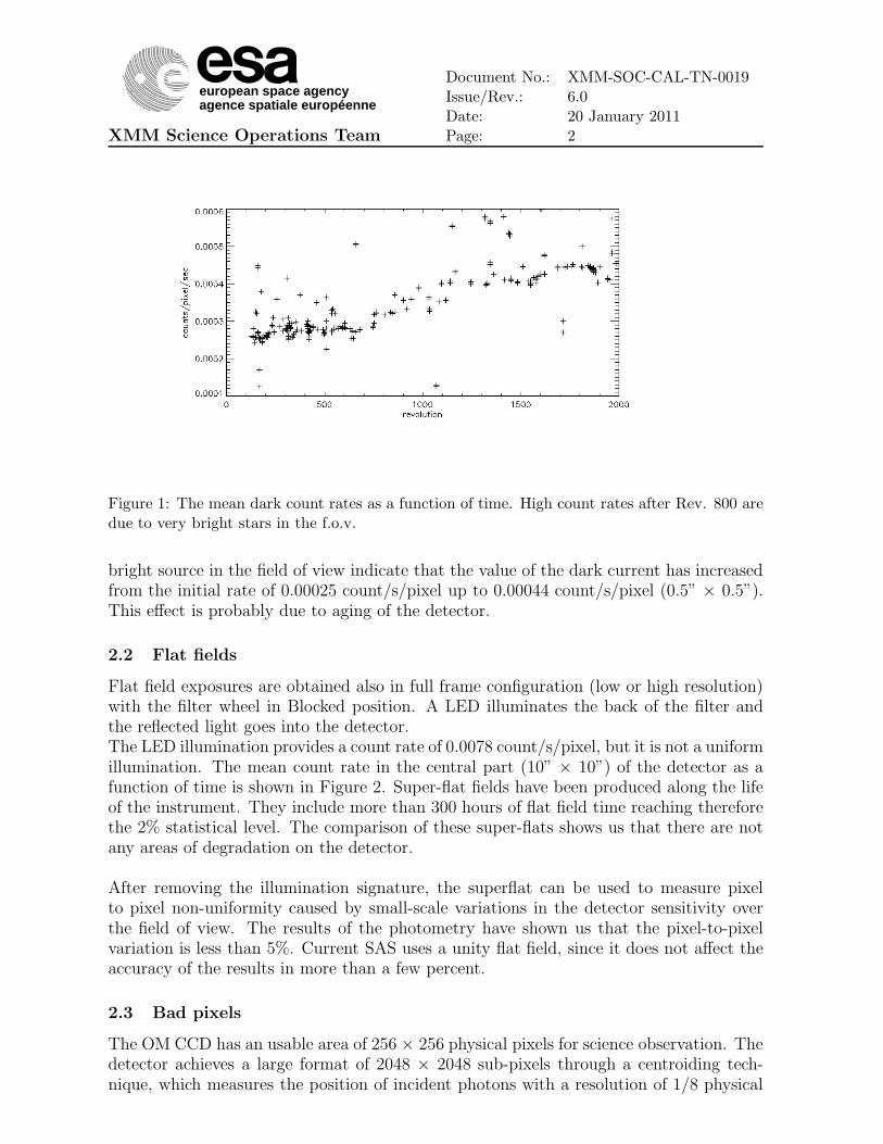
The dark frames are long exposures (4000 seconds) obtained in full frame configuration(low or high resolution) in the Blocked filter wheel position.The dark count rate is very low, of the order of 0.0004 count/s/pixel and its variationacross the detector is of the order of 7%. Figure 1 shows the mean dark count rate as afunction of time, which is being monitored routinely.Sometimes dark frames are obtained serendipitously when OM cannot be used scientifi-cally due to the presence of bright sources in the field of view. The large values visible inFigure 1 may be produced in these cases. Recent measurements performed in absence of




Figure 1: The mean dark count rates as a function of time. High count rates after Rev. 800 aredue to very bright stars in the f.o.v.

bright source in the field of view indicate that the value of the dark current has increasedfrom the initial rate of 0.00025 count/s/pixel up to 0.00044 count/s/pixel (0.5” × 0.5”).This effect is probably due to aging of the detector.

2.2 Flat fields

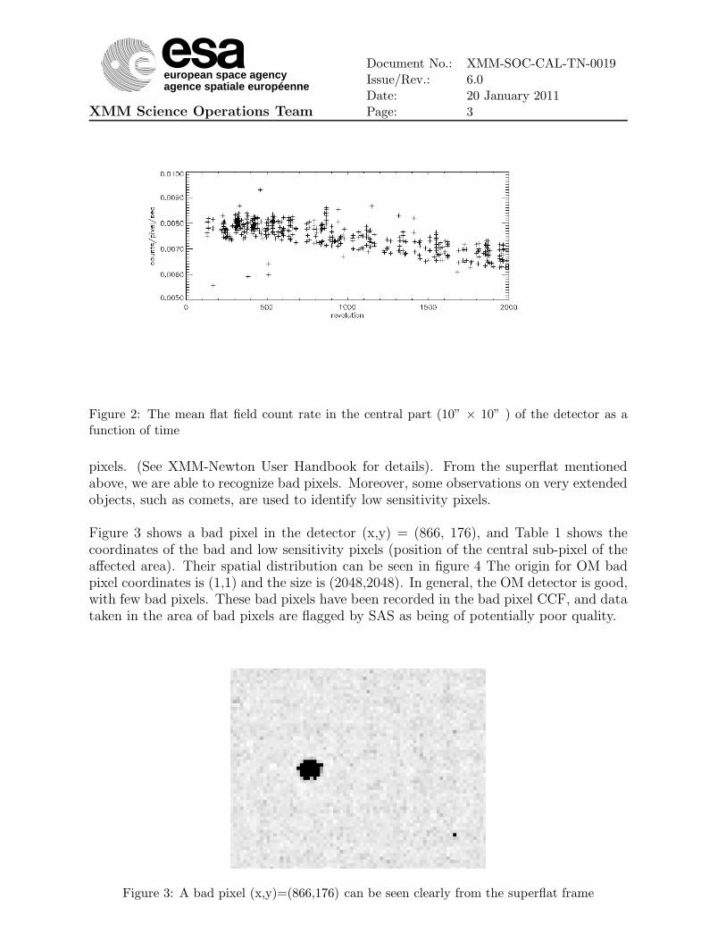
Flat field exposures are obtained also in full frame configuration (low or high resolution)with the filter wheel in Blocked position. A LED illuminates the back of the filter andthe reflected light goes into the detector.The LED illumination provides a count rate of 0.0078 count/s/pixel, but it is not a uniformillumination. The mean count rate in the central part (10” × 10”) of the detector as afunction of time is shown in Figure 2. Super-flat fields have been produced along the lifeof the instrument. They include more than 300 hours of flat field time reaching thereforethe 2% statistical level. The comparison of these super-flats shows us that there are notany areas of degradation on the detector.

After removing the illumination signature, the superflat can be used to measure pixelto pixel non-uniformity caused by small-scale variations in the detector sensitivity overthe field of view. The results of the photometry have shown us that the pixel-to-pixelvariation is less than 5%. Current SAS uses a unity flat field, since it does not affect theaccuracy of the results in more than a few percent.

2.3 Bad pixels

The OM CCD has an usable area of 256 × 256 physical pixels for science observation. Thedetector achieves a large format of 2048 × 2048 sub-pixels through a centroiding tech-nique, which measures the position of incident photons with a resolution of 1/8 physical




Figure 2: The mean flat field count rate in the central part (10” × 10” ) of the detector as afunction of time

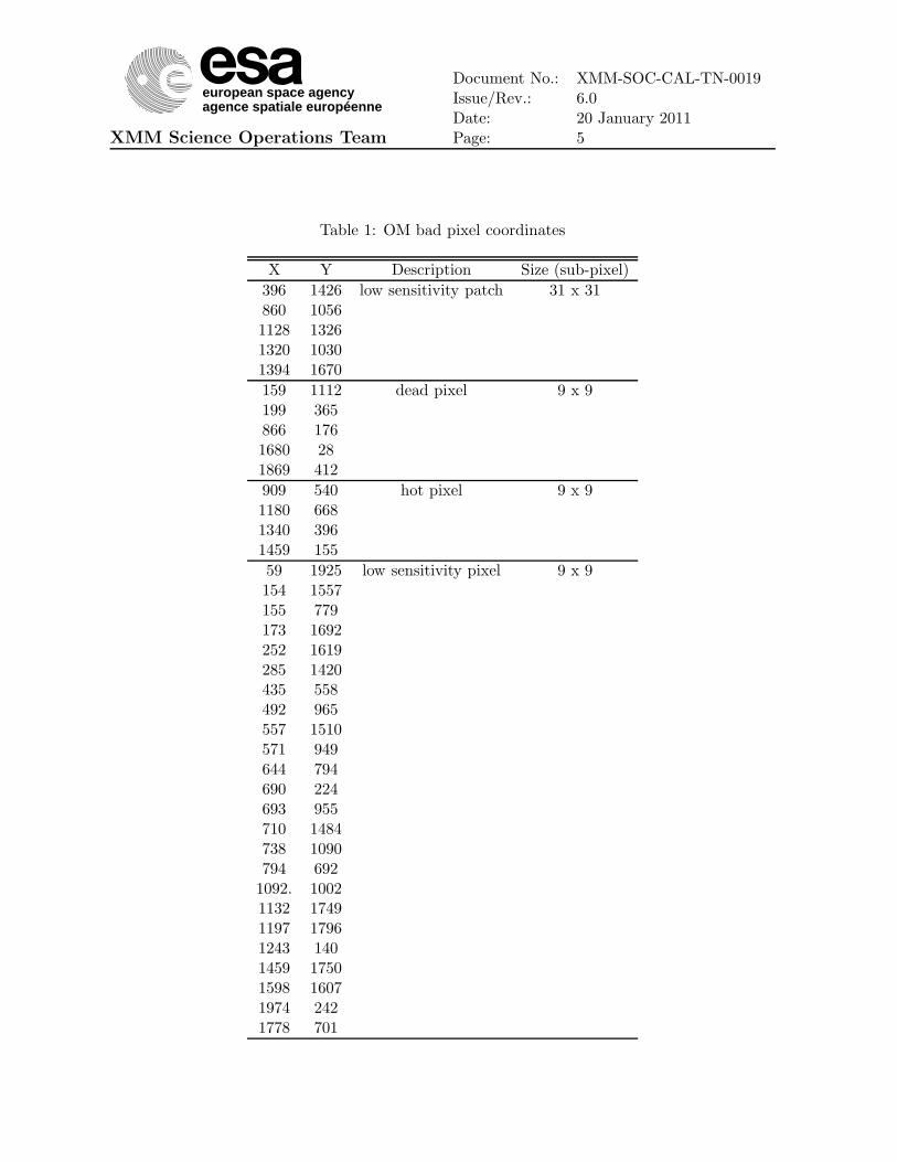
pixels. (See XMM-Newton User Handbook for details). From the superflat mentionedabove, we are able to recognize bad pixels. Moreover, some observations on very extendedobjects, such as comets, are used to identify low sensitivity pixels.

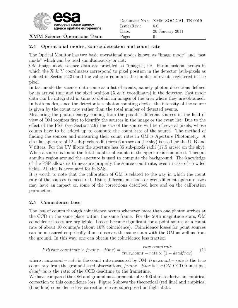
Figure 3 shows a bad pixel in the detector (x,y) = (866, 176), and Table 1 shows thecoordinates of the bad and low sensitivity pixels (position of the central sub-pixel of theaffected area). Their spatial distribution can be seen in figure 4 The origin for OM badpixel coordinates is (1,1) and the size is (2048,2048). In general, the OM detector is good,with few bad pixels. These bad pixels have been recorded in the bad pixel CCF, and datataken in the area of bad pixels are flagged by SAS as being of potentially poor quality.

Figure 3: A bad pixel (x,y)=(866,176) can be seen clearly from the superflat frame




0 500 1000 1500 2000

0

500

1000

1500

2000

RAWX (pixel)

RAWY (pixel)

OM_BADPIX_0005.CCF(RAWY_1-24749)

Figure 4: Distribution of bad pixels and low sensitivity areas in the OM detector




Table 1: OM bad pixel coordinates

X Y Description Size (sub-pixel)

396 1426 low sensitivity patch 31 x 31860 10561128 13261320 10301394 1670

159 1112 dead pixel 9 x 9199 365866 1761680 281869 412

909 540 hot pixel 9 x 91180 6681340 3961459 155

59 1925 low sensitivity pixel 9 x 9154 1557155 779173 1692252 1619285 1420435 558492 965557 1510571 949644 794690 224693 955710 1484738 1090794 692

1092. 10021132 17491197 17961243 1401459 17501598 16071974 2421778 701




2.4 Operational modes, source detection and count rate

The Optical Monitor has two basic operational modes known as “image mode” and “fastmode” which can be used simultaneously or not.OM image mode science data are provided as “images”, i.e. bi-dimensional arrays inwhich the X & Y coordinates correspond to pixel position in the detector (sub-pixels asdefined in Section 2.3) and the value or counts is the number of events registered in thepixel.In fast mode the science data come as a list of events, namely photon detections definedby its arrival time and the pixel position (X & Y coordinates) in the detector. Fast modedata can be integrated in time to obtain an images of the area where they are obtained.In both modes, since the detector is a photon counting device, the intensity of the sourceis given by the count rate rather than the total number of detected events.Measuring the photon energy coming from the possible different sources in the field ofview of OM requires first to identify the sources in the image or the event list. Due to theeffect of the PSF (see Section 2.6) the size of the source will be of several pixels, whosecounts have to be added up to compute the count rate of the source. The method offinding the sources and measuring their count rates in OM is Aperture Photometry. Acircular aperture of 12 sub-pixels radii (circa 6 arcsec on the sky) is used for the U, B andV filters. For the UV filters the aperture has 35 sub-pixels radii (17.5 arcsec on the sky).When a source is found the total number of counts in the aperture is computed. Then anannulus region around the aperture is used to compute the background. The knowledgeof the PSF allows us to measure properly the source count rate, even in case of crowdedfields. All this is accounted for in SAS.It is worth to note that the calibration of OM is related to the way in which the countrate of the sources is measured. Using different methods or even different aperture sizesmay have an impact on some of the corrections described here and on the calibrationparameters.

2.5 Coincidence Loss

The loss of counts through coincidence occurs whenever more than one photon arrives atthe CCD in the same place within the same frame. For the 20th magnitude stars, OMcoincidence losses are negligible. Losses become significant for a point source at a countrate of about 10 counts/s (about 10% coincidence). Coincidence losses for point sourcescan be measured empirically if one observes the same stars with the OM as well as fromthe ground. In this way, one can obtain the coincidence loss fraction

FR(raw countrate × frame − time) =raw countrate

true count − rate × (1 − deadfrac)(1)

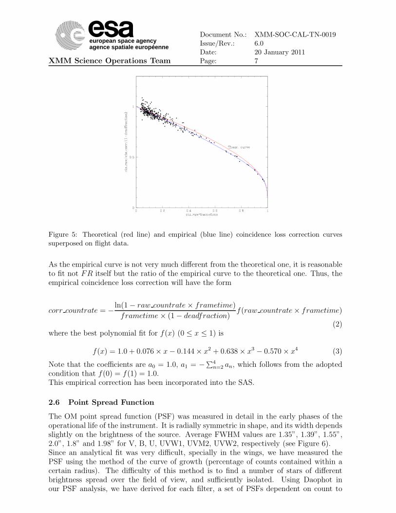
where raw count− rate is the count rate measured by OM, true count− rate is the truecount rate from the ground-based observations, frame−time is the OM CCD frametime,deadfrac is the ratio of the CCD deadtime to the frametime.We have compared the OM and ground measurements of ∼ 400 stars to derive an empiricalcorrection to this coincidence loss. Figure 5 shows the theoretical (red line) and empirical(blue line) coincidence loss correction curves superposed on flight data.




Figure 5: Theoretical (red line) and empirical (blue line) coincidence loss correction curvessuperposed on flight data.

As the empirical curve is not very much different from the theoretical one, it is reasonableto fit not FR itself but the ratio of the empirical curve to the theoretical one. Thus, theempirical coincidence loss correction will have the form

corr countrate = −ln(1 − raw countrate × frametime)

frametime × (1 − deadfraction)f(raw countrate× frametime)

(2)where the best polynomial fit for f(x) (0 ≤ x ≤ 1) is

f(x) = 1.0 + 0.076 × x − 0.144 × x2 + 0.638 × x3− 0.570 × x4 (3)

Note that the coefficients are a0 = 1.0, a1 = −∑

4

n=2an, which follows from the adopted

condition that f(0) = f(1) = 1.0.This empirical correction has been incorporated into the SAS.

2.6 Point Spread Function

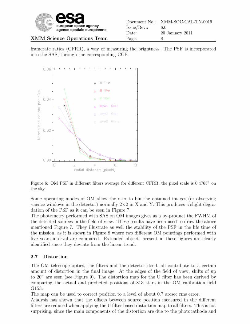
The OM point spread function (PSF) was measured in detail in the early phases of theoperational life of the instrument. It is radially symmetric in shape, and its width dependsslightly on the brightness of the source. Average FWHM values are 1.35”, 1.39”, 1.55”,2.0”, 1.8” and 1.98” for V, B, U, UVW1, UVM2, UVW2, respectively (see Figure 6).Since an analytical fit was very difficult, specially in the wings, we have measured thePSF using the method of the curve of growth (percentage of counts contained within acertain radius). The difficulty of this method is to find a number of stars of differentbrightness spread over the field of view, and sufficiently isolated. Using Daophot inour PSF analysis, we have derived for each filter, a set of PSFs dependent on count to




framerate ratios (CFRR), a way of measuring the brightness. The PSF is incorporatedinto the SAS, through the corresponding CCF.

Figure 6: OM PSF in different filters average for different CFRR, the pixel scale is 0.4765” onthe sky.

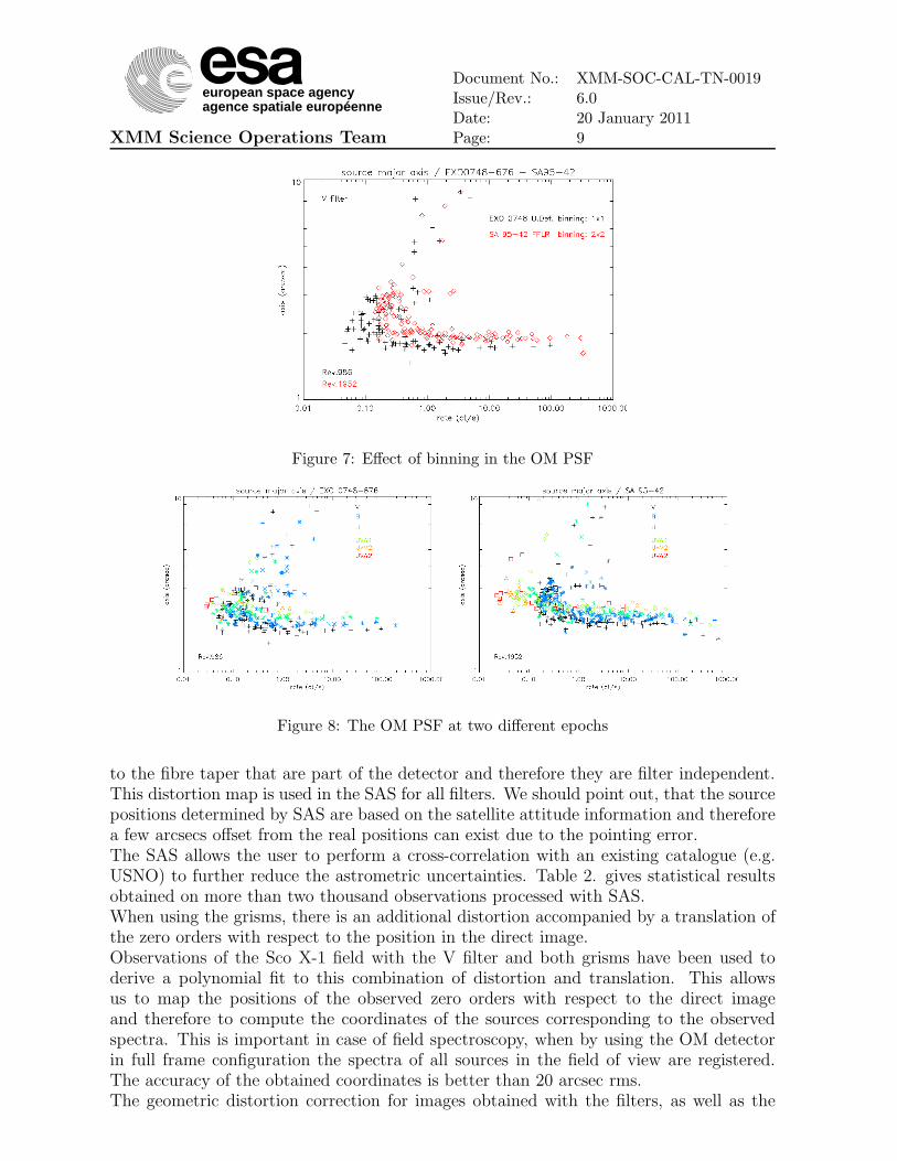
Some operating modes of OM allow the user to bin the obtained images (or observingscience windows in the detector) normally 2×2 in X and Y. This produces a slight degra-dation of the PSF as it can be seen in Figure 7.The photometry performed with SAS on OM images gives as a by-product the FWHM ofthe detected sources in the field of view. These results have been used to draw the abovementioned Figure 7. They illustrate as well the stability of the PSF in the life time ofthe mission, as it is shown in Figure 8 where two different OM pointings performed withfive years interval are compared. Extended objects present in these figures are clearlyidentified since they deviate from the linear trend.

2.7 Distortion

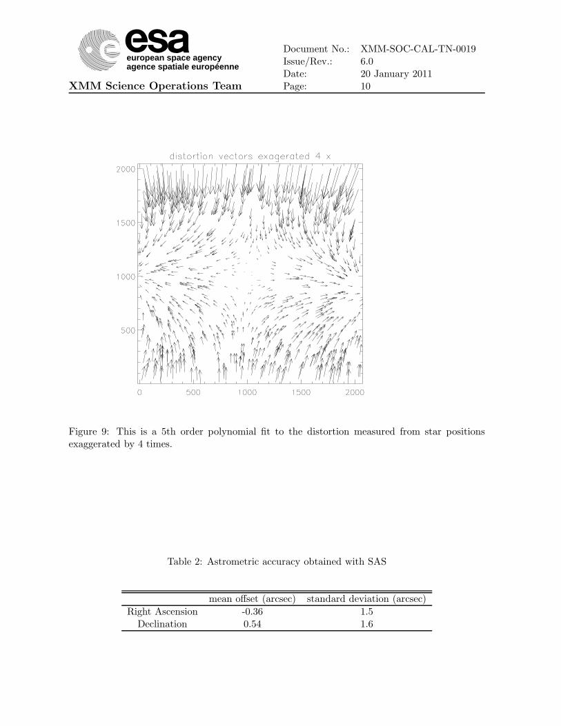
The OM telescope optics, the filters and the detector itself, all contribute to a certainamount of distortion in the final image. At the edges of the field of view, shifts of upto 20” are seen (see Figure 9). The distortion map for the U filter has been derived bycomparing the actual and predicted positions of 813 stars in the OM calibration fieldG153.The map can be used to correct position to a level of about 0.7 arcsec rms error.Analysis has shown that the offsets between source position measured in the differentfilters are reduced when applying the U filter based distortion map to all filters. This is notsurprising, since the main components of the distortion are due to the photocathode and




Figure 7: Effect of binning in the OM PSF

Figure 8: The OM PSF at two different epochs

to the fibre taper that are part of the detector and therefore they are filter independent.This distortion map is used in the SAS for all filters. We should point out, that the sourcepositions determined by SAS are based on the satellite attitude information and thereforea few arcsecs offset from the real positions can exist due to the pointing error.The SAS allows the user to perform a cross-correlation with an existing catalogue (e.g.USNO) to further reduce the astrometric uncertainties. Table 2. gives statistical resultsobtained on more than two thousand observations processed with SAS.When using the grisms, there is an additional distortion accompanied by a translation ofthe zero orders with respect to the position in the direct image.Observations of the Sco X-1 field with the V filter and both grisms have been used toderive a polynomial fit to this combination of distortion and translation. This allowsus to map the positions of the observed zero orders with respect to the direct imageand therefore to compute the coordinates of the sources corresponding to the observedspectra. This is important in case of field spectroscopy, when by using the OM detectorin full frame configuration the spectra of all sources in the field of view are registered.The accuracy of the obtained coordinates is better than 20 arcsec rms.The geometric distortion correction for images obtained with the filters, as well as the




Figure 9: This is a 5th order polynomial fit to the distortion measured from star positionsexaggerated by 4 times.

Table 2: Astrometric accuracy obtained with SAS

mean offset (arcsec) standard deviation (arcsec)

Right Ascension -0.36 1.5Declination 0.54 1.6




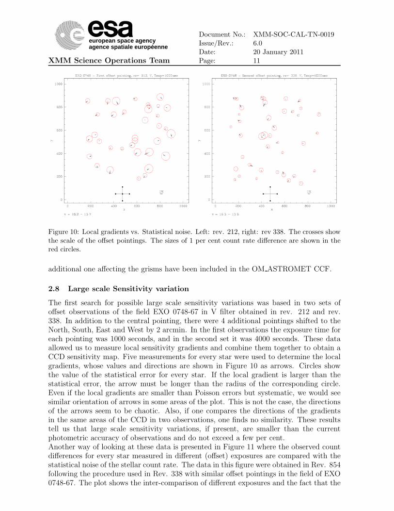
Figure 10: Local gradients vs. Statistical noise. Left: rev. 212, right: rev 338. The crosses showthe scale of the offset pointings. The sizes of 1 per cent count rate difference are shown in thered circles.

additional one affecting the grisms have been included in the OM ASTROMET CCF.

2.8 Large scale Sensitivity variation

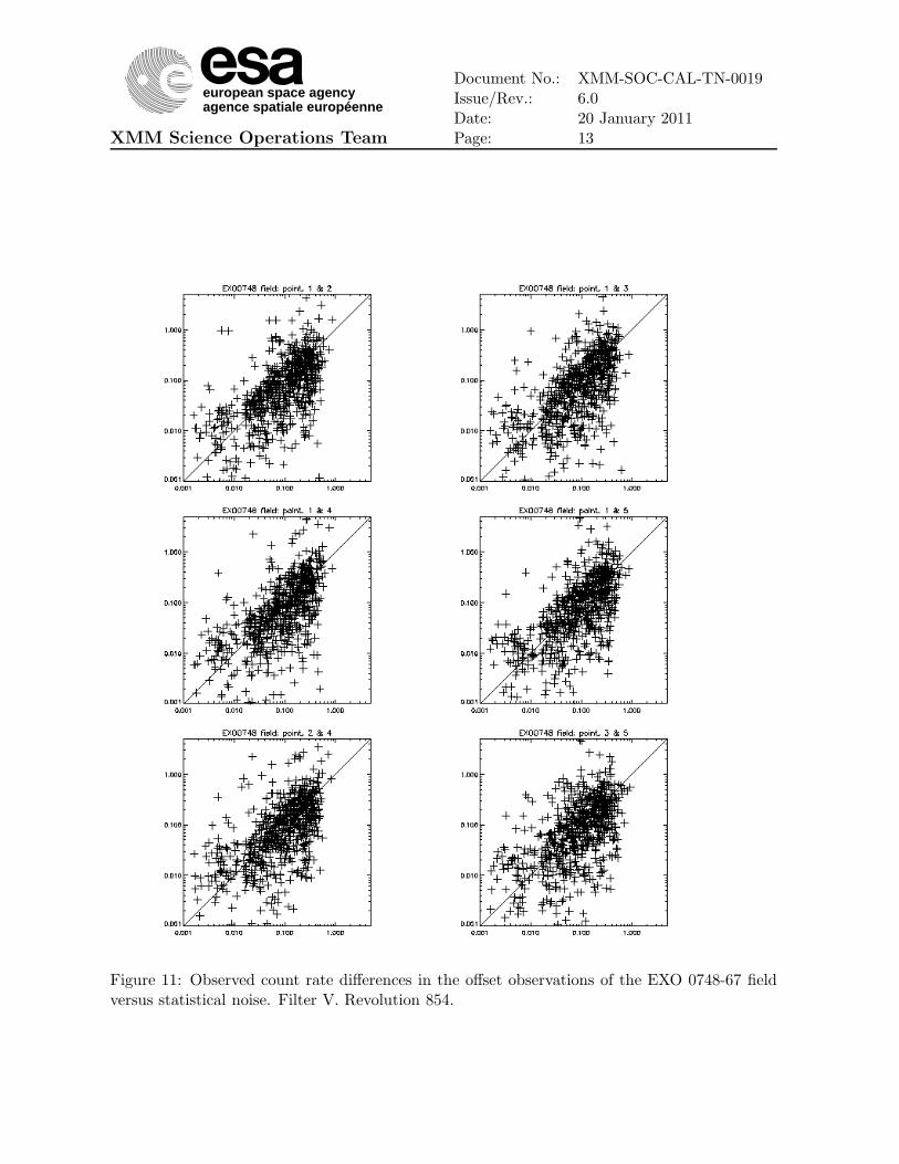
The first search for possible large scale sensitivity variations was based in two sets ofoffset observations of the field EXO 0748-67 in V filter obtained in rev. 212 and rev.338. In addition to the central pointing, there were 4 additional pointings shifted to theNorth, South, East and West by 2 arcmin. In the first observations the exposure time foreach pointing was 1000 seconds, and in the second set it was 4000 seconds. These dataallowed us to measure local sensitivity gradients and combine them together to obtain aCCD sensitivity map. Five measurements for every star were used to determine the localgradients, whose values and directions are shown in Figure 10 as arrows. Circles showthe value of the statistical error for every star. If the local gradient is larger than thestatistical error, the arrow must be longer than the radius of the corresponding circle.Even if the local gradients are smaller than Poisson errors but systematic, we would seesimilar orientation of arrows in some areas of the plot. This is not the case, the directionsof the arrows seem to be chaotic. Also, if one compares the directions of the gradientsin the same areas of the CCD in two observations, one finds no similarity. These resultstell us that large scale sensitivity variations, if present, are smaller than the currentphotometric accuracy of observations and do not exceed a few per cent.Another way of looking at these data is presented in Figure 11 where the observed countdifferences for every star measured in different (offset) exposures are compared with thestatistical noise of the stellar count rate. The data in this figure were obtained in Rev. 854following the procedure used in Rev. 338 with similar offset pointings in the field of EXO0748-67. The plot shows the inter-comparison of different exposures and the fact that the




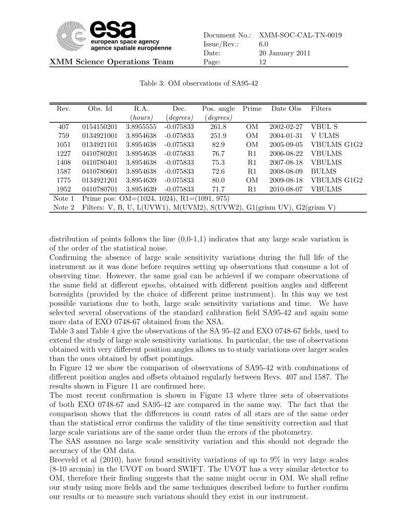
Table 3: OM observations of SA95-42

Rev. Obs. Id R.A. Dec. Pos. angle Prime Date Obs Filters(hours) (degrees) (degrees)

407 0154150201 3.8955555 -0.075833 261.8 OM 2002-02-27 VBUL S759 0134921001 3.8954638 -0.075833 251.9 OM 2004-01-31 V ULMS1051 0134921101 3.8954638 -0.075833 82.9 OM 2005-09-05 VBULMS G1G21227 0410780201 3.8954638 -0.075833 76.7 R1 2006-08-22 VBULMS1408 0410780401 3.8954638 -0.075833 75.3 R1 2007-08-18 VBULMS1587 0410780601 3.8954638 -0.075833 72.6 R1 2008-08-09 BULMS1775 0134921201 3.8954639 -0.075833 80.0 OM 2009-08-18 VBULMS G1G21952 0410780701 3.8954639 -0.075833 71.7 R1 2010-08-07 VBULMS

Note 1 Prime pos: OM=(1024, 1024), R1=(1091, 975)Note 2 Filters: V, B, U, L(UVW1), M(UVM2), S(UVW2), G1(grism UV), G2(grism V)

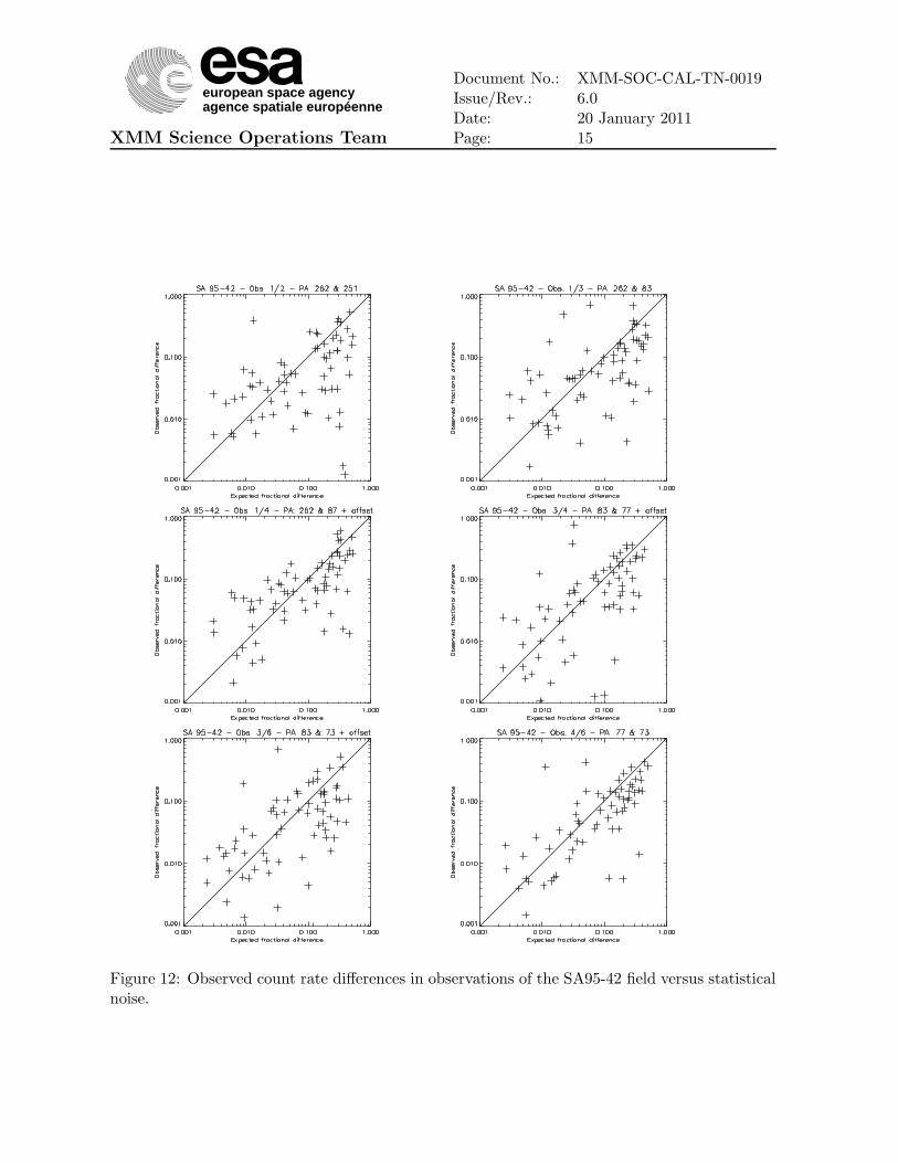
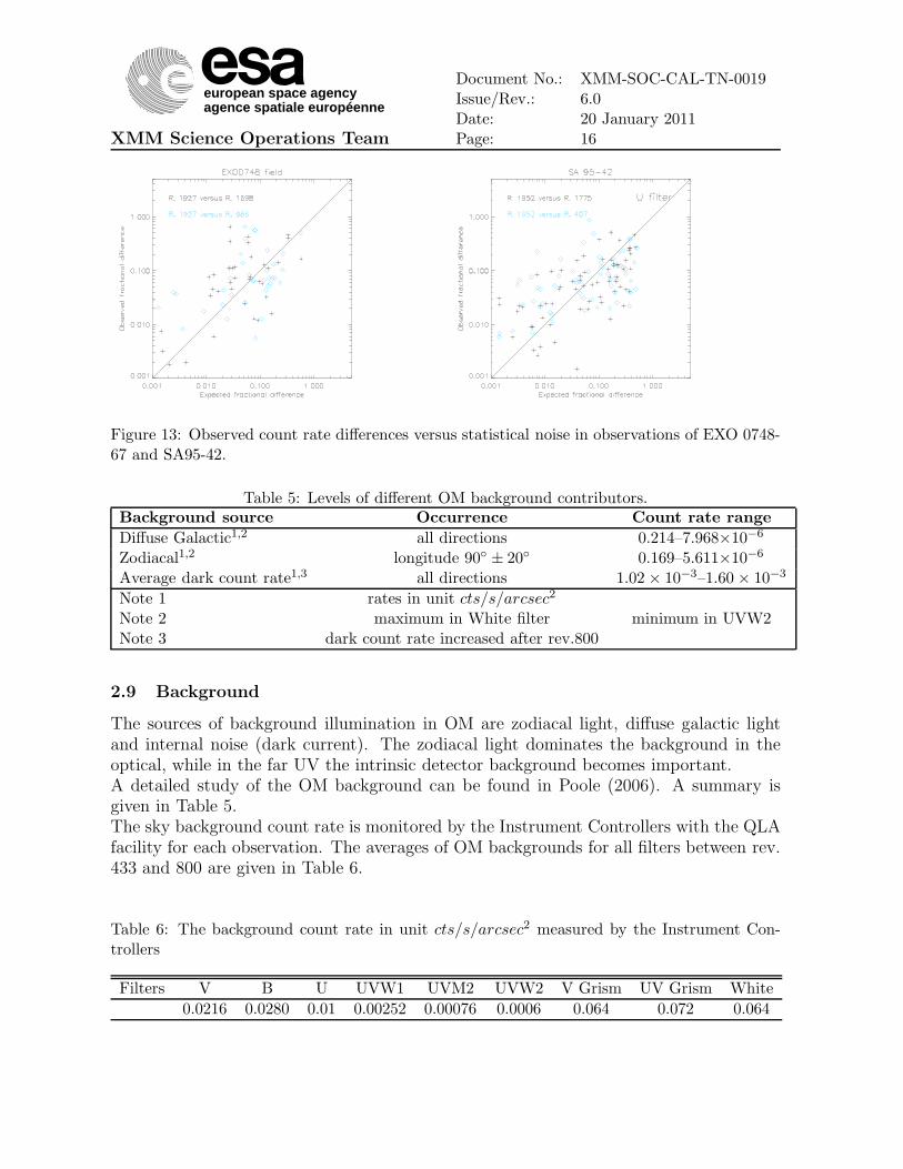
distribution of points follows the line (0,0-1,1) indicates that any large scale variation isof the order of the statistical noise.Confirming the absence of large scale sensitivity variations during the full life of theinstrument as it was done before requires setting up observations that consume a lot ofobserving time. However, the same goal can be achieved if we compare observations ofthe same field at different epochs, obtained with different position angles and differentboresights (provided by the choice of different prime instrument). In this way we testpossible variations due to both, large scale sensitivity variations and time. We haveselected several observations of the standard calibration field SA95-42 and again somemore data of EXO 0748-67 obtained from the XSA.Table 3 and Table 4 give the observations of the SA 95-42 and EXO 0748-67 fields, used toextend the study of large scale sensitivity variations. In particular, the use of observationsobtained with very different position angles allows us to study variations over larger scalesthan the ones obtained by offset pointings.In Figure 12 we show the comparison of observations of SA95-42 with combinations ofdifferent position angles and offsets obtained regularly between Revs. 407 and 1587. Theresults shown in Figure 11 are confirmed here.The most recent confirmation is shown in Figure 13 where three sets of observationsof both EXO 0748-67 and SA95-42 are compared in the same way. The fact that thecomparison shows that the differences in count rates of all stars are of the same orderthan the statistical error confirms the validity of the time sensitivity correction and thatlarge scale variations are of the same order than the errors of the photometry.The SAS assumes no large scale sensitivity variation and this should not degrade theaccuracy of the OM data.Breeveld et al (2010), have found sensitivity variations of up to 9% in very large scales(8-10 arcmin) in the UVOT on board SWIFT. The UVOT has a very similar detector toOM, therefore their finding suggests that the same might occur in OM. We shall refineour study using more fields and the same techniques described before to further confirmour results or to measure such variatons should they exist in our instrument.




Figure 11: Observed count rate differences in the offset observations of the EXO 0748-67 fieldversus statistical noise. Filter V. Revolution 854.




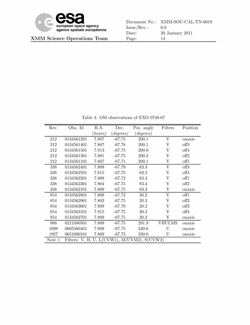
Table 4: OM observations of EXO 0748-67

Rev. Obs. Id R.A. Dec. Pos. angle Filters Position(hours) (degrees) (degrees)

212 0134561201 7.807 -67.75 200.1 V onaxis212 0134561401 7.807 -67.78 200.1 V off3212 0134561501 7.813 -67.75 200.0 V off4212 0134561301 7.801 -67.75 200.2 V off2212 0134561101 7.807 -67.71 200.1 V off1

338 0134562401 7.809 -67.79 83.3 V off3338 0134562501 7.815 -67.75 83.2 V off4338 0134562201 7.809 -67.72 83.3 V off1338 0134562301 7.804 -67.75 83.4 V off2338 0134562101 7.809 -67.75 83.3 V onaxis

854 0134562801 7.809 -67.72 20.2 V off1854 0134562901 7.803 -67.75 20.3 V off2854 0134563001 7.809 -67.79 20.2 V off3854 0134563101 7.815 -67.75 20.2 V off4854 0134562701 7.809 -67.75 20.2 V onaxis

986 0212480501 7.809 -67.75 281.9 VBULMS onaxis1698 0605560401 7.809 -67.75 240.6 U onaxis1927 0651690101 7.809 -67.75 330.0 U onaxis

Note 1 Filters: V, B, U, L(UVW1), M(UVM2), S(UVW2)




Figure 12: Observed count rate differences in observations of the SA95-42 field versus statisticalnoise.




Figure 13: Observed count rate differences versus statistical noise in observations of EXO 0748-67 and SA95-42.

Table 5: Levels of different OM background contributors.Background source Occurrence Count rate range

Diffuse Galactic1,2 all directions 0.214–7.968×10−6

Zodiacal1,2 longitude 90◦ ± 20◦ 0.169–5.611×10−6

Average dark count rate1,3 all directions 1.02 × 10−3–1.60 × 10−3

Note 1 rates in unit cts/s/arcsec2

Note 2 maximum in White filter minimum in UVW2Note 3 dark count rate increased after rev.800

2.9 Background

The sources of background illumination in OM are zodiacal light, diffuse galactic lightand internal noise (dark current). The zodiacal light dominates the background in theoptical, while in the far UV the intrinsic detector background becomes important.A detailed study of the OM background can be found in Poole (2006). A summary isgiven in Table 5.The sky background count rate is monitored by the Instrument Controllers with the QLAfacility for each observation. The averages of OM backgrounds for all filters between rev.433 and 800 are given in Table 6.

Table 6: The background count rate in unit cts/s/arcsec2 measured by the Instrument Con-trollers

Filters V B U UVW1 UVM2 UVW2 V Grism UV Grism White

0.0216 0.0280 0.01 0.00252 0.00076 0.0006 0.064 0.072 0.064




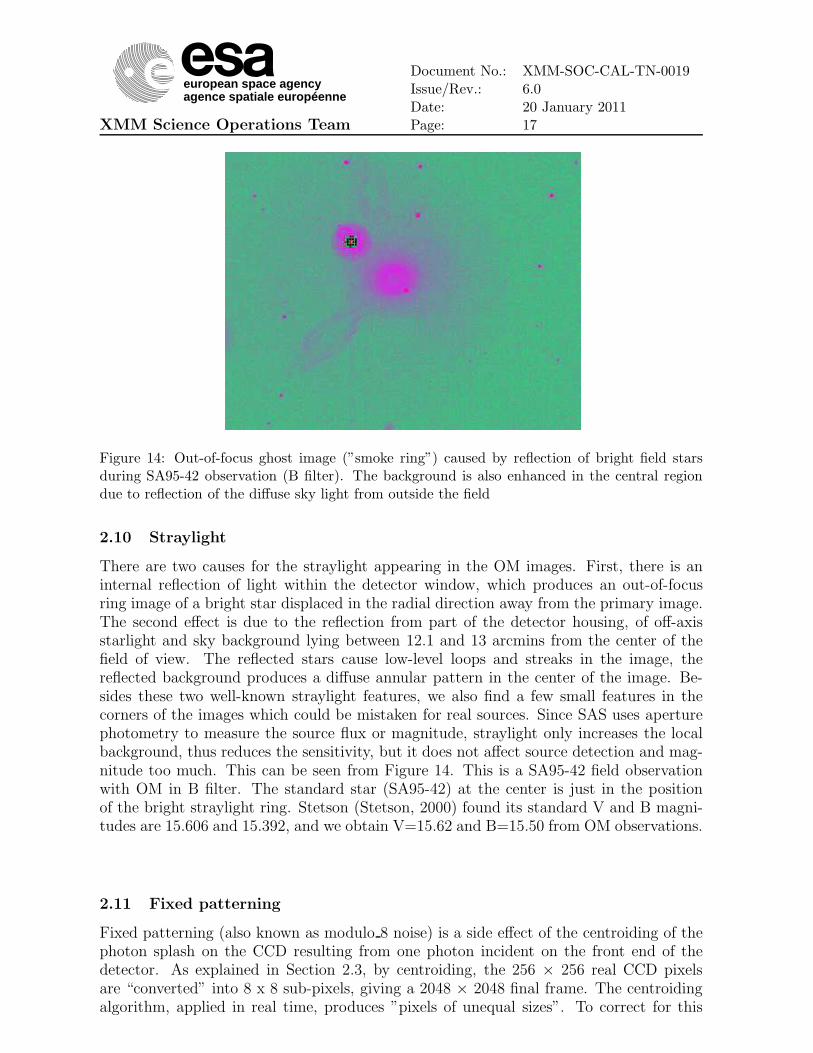
Figure 14: Out-of-focus ghost image (”smoke ring”) caused by reflection of bright field starsduring SA95-42 observation (B filter). The background is also enhanced in the central regiondue to reflection of the diffuse sky light from outside the field

2.10 Straylight

There are two causes for the straylight appearing in the OM images. First, there is aninternal reflection of light within the detector window, which produces an out-of-focusring image of a bright star displaced in the radial direction away from the primary image.The second effect is due to the reflection from part of the detector housing, of off-axisstarlight and sky background lying between 12.1 and 13 arcmins from the center of thefield of view. The reflected stars cause low-level loops and streaks in the image, thereflected background produces a diffuse annular pattern in the center of the image. Be-sides these two well-known straylight features, we also find a few small features in thecorners of the images which could be mistaken for real sources. Since SAS uses aperturephotometry to measure the source flux or magnitude, straylight only increases the localbackground, thus reduces the sensitivity, but it does not affect source detection and mag-nitude too much. This can be seen from Figure 14. This is a SA95-42 field observationwith OM in B filter. The standard star (SA95-42) at the center is just in the positionof the bright straylight ring. Stetson (Stetson, 2000) found its standard V and B magni-tudes are 15.606 and 15.392, and we obtain V=15.62 and B=15.50 from OM observations.

2.11 Fixed patterning

Fixed patterning (also known as modulo 8 noise) is a side effect of the centroiding of thephoton splash on the CCD resulting from one photon incident on the front end of thedetector. As explained in Section 2.3, by centroiding, the 256 × 256 real CCD pixelsare “converted” into 8 x 8 sub-pixels, giving a 2048 × 2048 final frame. The centroidingalgorithm, applied in real time, produces ”pixels of unequal sizes”. To correct for this




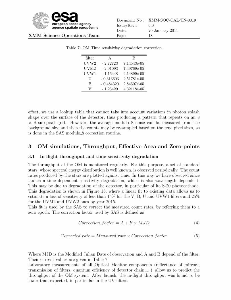
Table 7: OM Time sensitivity degradation correction

filter A B

UVW2 - 2.72723 7.14543e-05UVM2 - 2.91093 7.49769e-05UVW1 - 1.16448 4.14899e-05

U - 0.313603 2.51781e-05B - 0.484320 2.84507e-05V - 1.25429 4.32118e-05

effect, we use a lookup table that cannot take into account variations in photon splashshape over the surface of the detector, thus producing a pattern that repeats on an 8× 8 sub-pixel grid. However, the average modulo 8 noise can be measured from thebackground sky, and then the counts may be re-sampled based on the true pixel sizes, asis done in the SAS modulo 8 correction routine.

3 OM simulations, Throughput, Effective Area and Zero-points

3.1 In-flight throughput and time sensitivity degradation

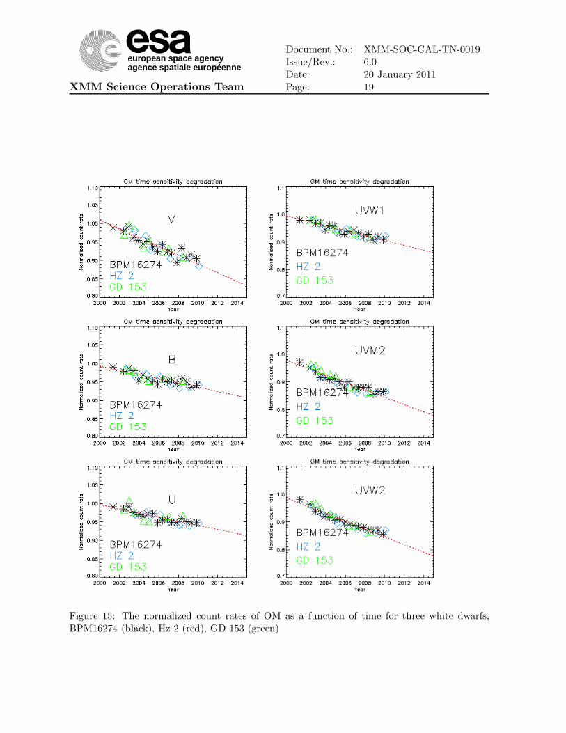
The throughput of the OM is monitored regularly. For this purpose, a set of standardstars, whose spectral energy distribution is well known, is observed periodically. The countrates produced by the stars are plotted against time. In this way we have observed sincelaunch a time dependent sensitivity degradation, which is also wavelength dependent.This may be due to degradation of the detector, in particular of its S-20 photocathode.This degradation is shown in Figure 15, where a linear fit to existing data allows us toestimate a loss of sensitivity of less than 15% for the V, B, U and UVW1 filters and 25%for the UVM2 and UVW2 ones by year 2015.This fit is used by the SAS to correct the measured count rates, by referring them to azero epoch. The correction factor used by SAS is defined as

Correction factor = A + B × MJD (4)

Corrected rate = Measured rate × Correction factor (5)

Where MJD is the Modified Julian Date of observation and A and B depend of the filter.Their current values are given in Table 7.Laboratory measurements of all Optical Monitor components (reflectance of mirrors,transmission of filters, quantum efficiency of detector chain,....) allow us to predict thethroughput of the OM system. After launch, the in-flight throughput was found to belower than expected, in particular in the UV filters.




Figure 15: The normalized count rates of OM as a function of time for three white dwarfs,BPM16274 (black), Hz 2 (red), GD 153 (green)




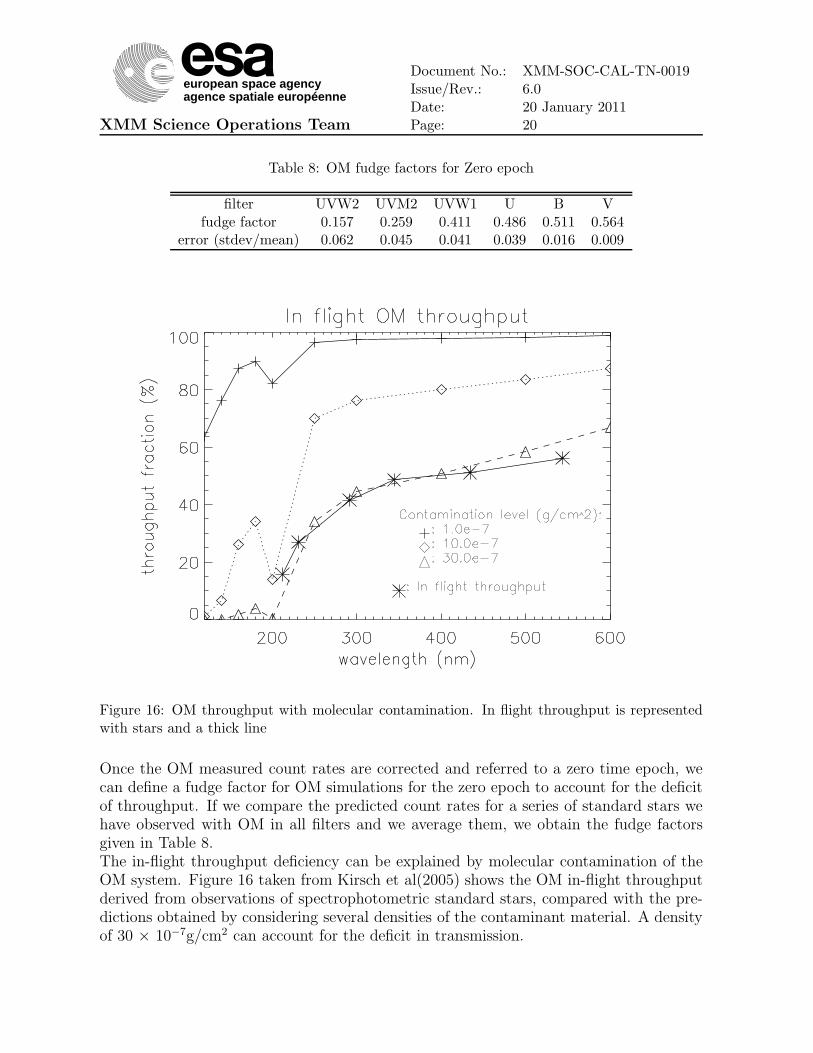
Table 8: OM fudge factors for Zero epoch

filter UVW2 UVM2 UVW1 U B Vfudge factor 0.157 0.259 0.411 0.486 0.511 0.564

error (stdev/mean) 0.062 0.045 0.041 0.039 0.016 0.009

Figure 16: OM throughput with molecular contamination. In flight throughput is representedwith stars and a thick line

Once the OM measured count rates are corrected and referred to a zero time epoch, wecan define a fudge factor for OM simulations for the zero epoch to account for the deficitof throughput. If we compare the predicted count rates for a series of standard stars wehave observed with OM in all filters and we average them, we obtain the fudge factorsgiven in Table 8.The in-flight throughput deficiency can be explained by molecular contamination of theOM system. Figure 16 taken from Kirsch et al(2005) shows the OM in-flight throughputderived from observations of spectrophotometric standard stars, compared with the pre-dictions obtained by considering several densities of the contaminant material. A densityof 30 × 10−7g/cm2 can account for the deficit in transmission.




Table 9: Measured count rates (cts/s) versus predictions using the OM effective areas

BPM 16274

filter UVW2 UVM2 UVW1 U B V Whitepredicted rate 14.3 29.2 72.3 109.0 107.0 32.1 481.observed rate 14.7 30.4 72.9 113.0 107.9 32.6 436.difference (%) 2.8 4.1 0.8 3.7 0.8 1.6 -9.5

3.2 Effective areas and response matrices

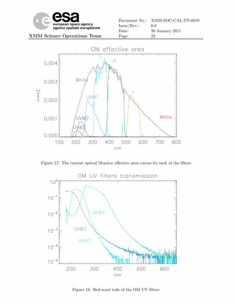
Computing the effective area of the OM system needs to take into account the contributionof all elements, mirrors, filters, detector chain,..., and also the throughput deficiency. Thelatter is taken into account by fitting a polynomial to the measured fudge factors for eachfilter. When this is done, and we use the effective area to predict the count rate of theobserved standard stars, we need to further adjust the fudge for the UV filters. This isdone by an additional factor in the UVW1 and UVM2 filters. The difference with theobservations achieved by this final effective area can be seen in Table 9 where we comparethe measurements of the standard star BPM 16274 (mean of 19 observations spread alongthe life of the instrument) with the predictions obtained using the effective areas.Figure 17 shows the OM effective area for all filters.Response matrices to be used in XSpec type environments have been derived from theeffective area.

3.2.1 The White filter.

Since there were no OM observations of our standards with the White filter because oftheir brightness, we have taken the polynomial fit for the molecular contamination and wehave combined it with the laboratory measurements of the filter and all other elements.We are observing the standard star BPM 16274 with the white filter since Rev.1449. Inspite of the big coincidence losses (count rate above 400 c/s) the simulations using thewhite filter effective area agree with the measured values within less than 10 % (see Table9). Since no correction for time dependent sensitivity degradation is applied in the caseof the White filter, this difference might be due to the absence of such correction. Themeasurements obtained with that filter cover barely three years and no correction can bederived from them.

3.3 Red leak in UV filters

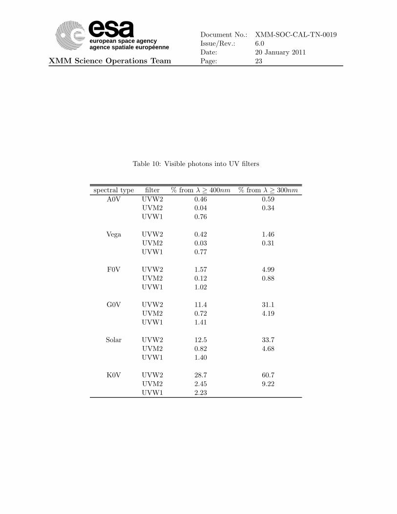
The OM UV filters (see Fig.18) transmissions have very faint red-ward tails. Even if theyare a few orders of magnitude smaller than the filter transmission peak, their contributionto the measured count rate can be significant in case of very cool objects with little fluxin the UV but bright in the visible range, e.g. K or M type stars. Table 10 shows thatfor a K0V star, the UVW2 counts due to photons of wavelengths beyond 4000 A can beas high as 29 % and 60 % from beyond 3000 A.




Figure 17: The current optical Monitor effective area curves for each of the filters

Figure 18: Red-ward tails of the OM UV filters




Table 10: Visible photons into UV filters

spectral type filter % from λ ≥ 400nm % from λ ≥ 300nm

A0V UVW2 0.46 0.59UVM2 0.04 0.34UVW1 0.76

Vega UVW2 0.42 1.46UVM2 0.03 0.31UVW1 0.77

F0V UVW2 1.57 4.99UVM2 0.12 0.88UVW1 1.02

G0V UVW2 11.4 31.1UVM2 0.72 4.19UVW1 1.41

Solar UVW2 12.5 33.7UVM2 0.82 4.68UVW1 1.40

K0V UVW2 28.7 60.7UVM2 2.45 9.22UVW1 2.23




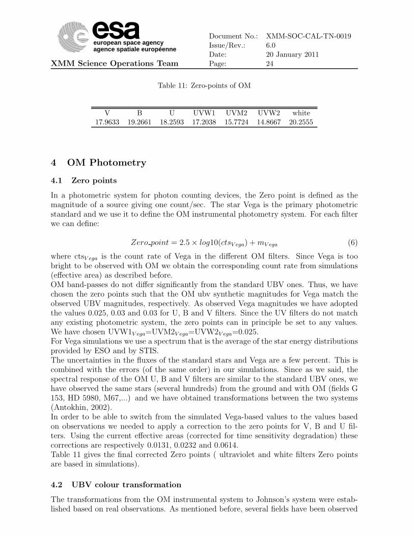
Table 11: Zero-points of OM

V B U UVW1 UVM2 UVW2 white17.9633 19.2661 18.2593 17.2038 15.7724 14.8667 20.2555

4 OM Photometry

4.1 Zero points

In a photometric system for photon counting devices, the Zero point is defined as themagnitude of a source giving one count/sec. The star Vega is the primary photometricstandard and we use it to define the OM instrumental photometry system. For each filterwe can define:

Zero point = 2.5 × log10(ctsV ega) + mV ega (6)

where ctsV ega is the count rate of Vega in the different OM filters. Since Vega is toobright to be observed with OM we obtain the corresponding count rate from simulations(effective area) as described before.OM band-passes do not differ significantly from the standard UBV ones. Thus, we havechosen the zero points such that the OM ubv synthetic magnitudes for Vega match theobserved UBV magnitudes, respectively. As observed Vega magnitudes we have adoptedthe values 0.025, 0.03 and 0.03 for U, B and V filters. Since the UV filters do not matchany existing photometric system, the zero points can in principle be set to any values.We have chosen UVW1V ega=UVM2V ega=UVW2V ega=0.025.For Vega simulations we use a spectrum that is the average of the star energy distributionsprovided by ESO and by STIS.The uncertainties in the fluxes of the standard stars and Vega are a few percent. This iscombined with the errors (of the same order) in our simulations. Since as we said, thespectral response of the OM U, B and V filters are similar to the standard UBV ones, wehave observed the same stars (several hundreds) from the ground and with OM (fields G153, HD 5980, M67,...) and we have obtained transformations between the two systems(Antokhin, 2002).In order to be able to switch from the simulated Vega-based values to the values basedon observations we needed to apply a correction to the zero points for V, B and U fil-ters. Using the current effective areas (corrected for time sensitivity degradation) thesecorrections are respectively 0.0131, 0.0232 and 0.0614.Table 11 gives the final corrected Zero points ( ultraviolet and white filters Zero pointsare based in simulations).

4.2 UBV colour transformation

The transformations from the OM instrumental system to Johnson’s system were estab-lished based on real observations. As mentioned before, several fields have been observed




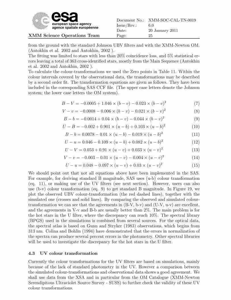
from the ground with the standard Johnson UBV filters and with the XMM-Newton OM.(Antokhin et al. 2002 and Antokhin, 2002 ).The fitting was limited to stars with less than 20% coincidence loss, and 5% statistical er-rors leaving a total of 363 cross-identified stars, mostly from the Main Sequence (Antokhinet al. 2002 and Antokhin, 2002 ).To calculate the colour-transformations we used the Zero points in Table 11. Within thecolour intervals covered by the observational data, the transformations may be describedby a second order fit. The transformation equations are given as follows. They have beenincluded in the corresponding SAS CCF file. (The upper case letters denote the Johnsonsystem; the lower case letters the OM system).

B − V = −0.0005 + 1.046 × (b − v) − 0.023 × (b − v)2 (7)

V − v = −0.0008 − 0.006 × (b − v) − 0.021 × (b − v)2 (8)

B − b = −0.0014 + 0.04 × (b − v) − 0.044 × (b − v)2 (9)

U − B = −0.002 + 0.901 × (u − b) + 0.103 × (u − b)2 (10)

B − b = 0.0078 − 0.01 × (u − b) − 0.019 × (u − b)2 (11)

U − u = 0.046 − 0.109 × (u − b) + 0.082 × (u − b)2 (12)

U − V = 0.053 + 0.91 × (u − v) + 0.033 × (u − v)2 (13)

V − v = −0.003 − 0.01 × (u − v) − 0.004 × (u − v)2 (14)

U − u = 0.048 − 0.097 × (u − v) + 0.03 × (u − v)2 (15)

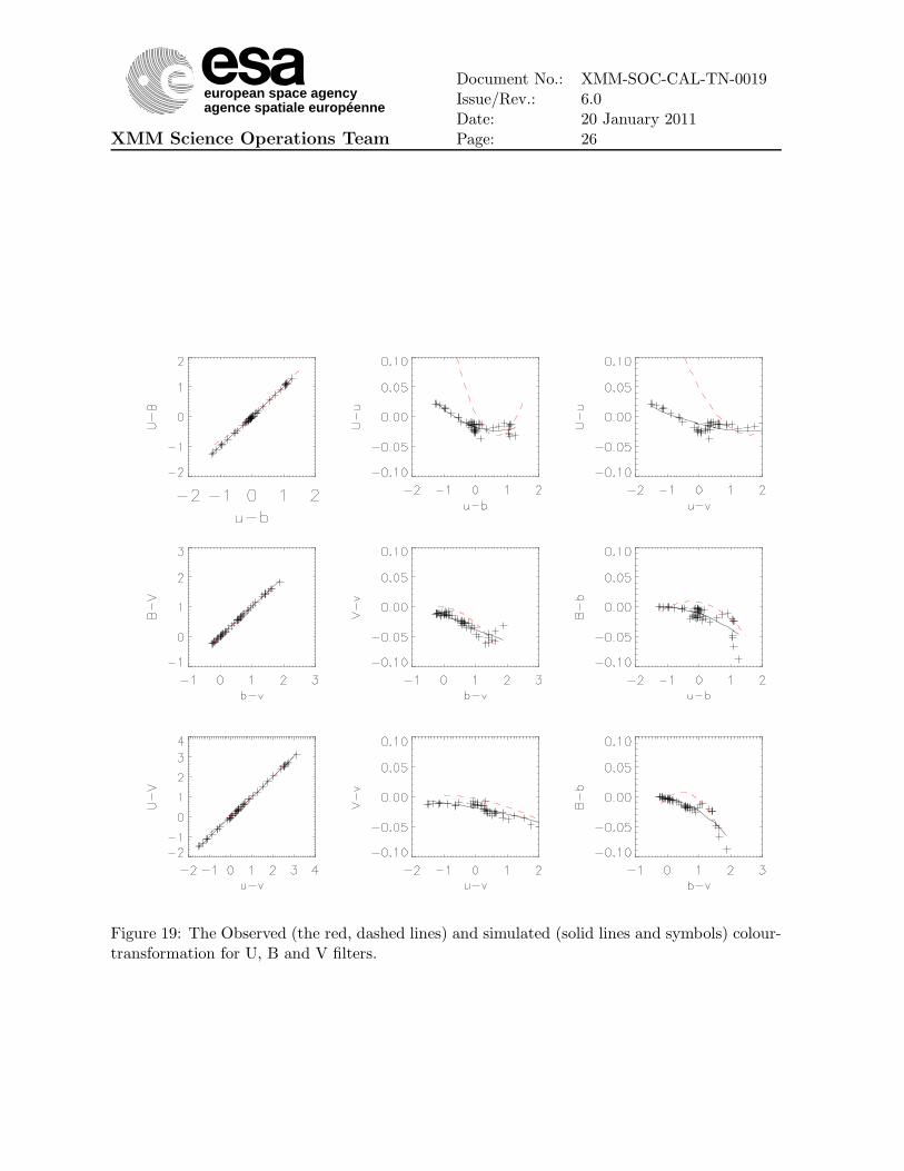
We should point out that not all equations above have been implemented in the SAS.For example, for deriving standard B magnitude, SAS uses (u-b) colour transformation(eq. 11), or making use of the UV filters (see next section). However, users can alsouse (b-v) colour transformation (eq. 9) to get standard B magnitude. In Figure 19, weplot the observed UBV colour-transformation (the red dashed lines), together with thesimulated one (crosses and solid lines). By comparing the observed and simulated colour-transformation we can see that the agreements in (B-V, b-v) and (U-V, u-v) are excellent,and the agreements in V-v and B-b are usually better than 2%. The main problem is forthe hot stars in the U filter, where the discrepancy can reach 10%. The spectral library(BPGS) used in the simulations is combined from several sources. For the optical data,the spectral atlas is based on Gunn and Stryker (1983) observations, which begins from313 nm. Colina and Bohlin (1994) have demonstrated that the errors in normalization ofthe spectra can produce several percent errors in the photometry. Other spectral librarieswill be used to investigate the discrepancy for the hot stars in the U filter.

4.3 UV colour transformation

Currently the colour transformations for the UV filters are based on simulations, mainlybecause of the lack of standard photometry in the UV. However a comparison betweenthe simulated colour-transformations and observational data shows a good agreement. Weshall use data from the XSA and in particular from the OM Catalogue (XMM-NewtonSerendipitous Ultraviolet Source Survey - SUSS) to further check the validity of these UVcolour transformations.




Figure 19: The Observed (the red, dashed lines) and simulated (solid lines and symbols) colour-transformation for U, B and V filters.




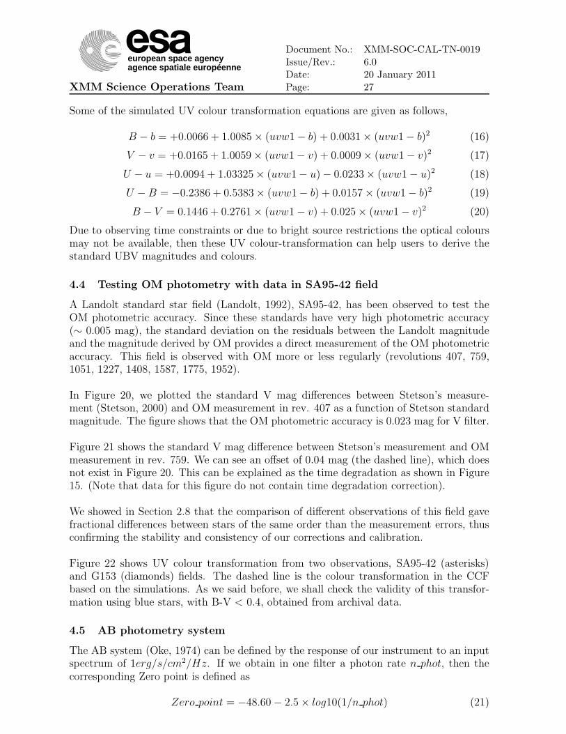
Some of the simulated UV colour transformation equations are given as follows,

B − b = +0.0066 + 1.0085 × (uvw1 − b) + 0.0031 × (uvw1− b)2 (16)

V − v = +0.0165 + 1.0059 × (uvw1 − v) + 0.0009 × (uvw1 − v)2 (17)

U − u = +0.0094 + 1.03325 × (uvw1− u) − 0.0233 × (uvw1− u)2 (18)

U − B = −0.2386 + 0.5383 × (uvw1− b) + 0.0157 × (uvw1 − b)2 (19)

B − V = 0.1446 + 0.2761 × (uvw1 − v) + 0.025 × (uvw1 − v)2 (20)

Due to observing time constraints or due to bright source restrictions the optical coloursmay not be available, then these UV colour-transformation can help users to derive thestandard UBV magnitudes and colours.

4.4 Testing OM photometry with data in SA95-42 field

A Landolt standard star field (Landolt, 1992), SA95-42, has been observed to test theOM photometric accuracy. Since these standards have very high photometric accuracy(∼ 0.005 mag), the standard deviation on the residuals between the Landolt magnitudeand the magnitude derived by OM provides a direct measurement of the OM photometricaccuracy. This field is observed with OM more or less regularly (revolutions 407, 759,1051, 1227, 1408, 1587, 1775, 1952).

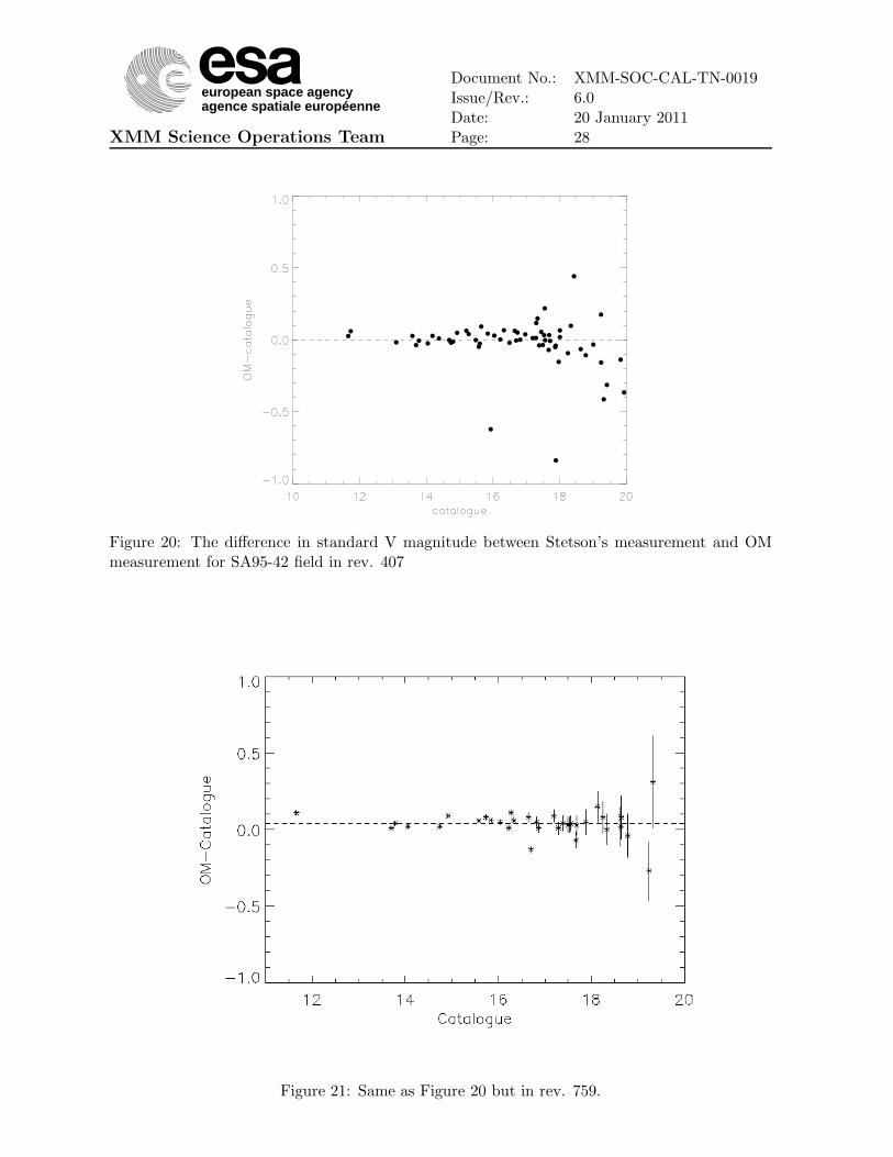
In Figure 20, we plotted the standard V mag differences between Stetson’s measure-ment (Stetson, 2000) and OM measurement in rev. 407 as a function of Stetson standardmagnitude. The figure shows that the OM photometric accuracy is 0.023 mag for V filter.

Figure 21 shows the standard V mag difference between Stetson’s measurement and OMmeasurement in rev. 759. We can see an offset of 0.04 mag (the dashed line), which doesnot exist in Figure 20. This can be explained as the time degradation as shown in Figure15. (Note that data for this figure do not contain time degradation correction).

We showed in Section 2.8 that the comparison of different observations of this field gavefractional differences between stars of the same order than the measurement errors, thusconfirming the stability and consistency of our corrections and calibration.

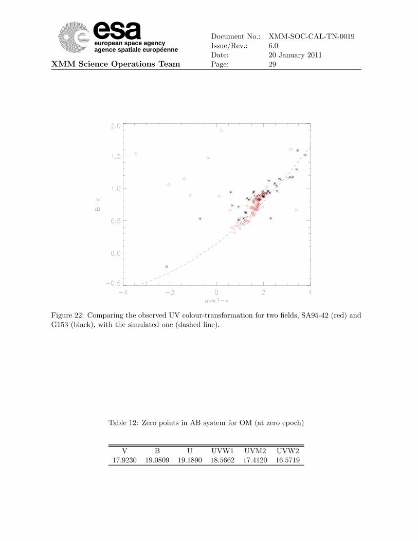
Figure 22 shows UV colour transformation from two observations, SA95-42 (asterisks)and G153 (diamonds) fields. The dashed line is the colour transformation in the CCFbased on the simulations. As we said before, we shall check the validity of this transfor-mation using blue stars, with B-V < 0.4, obtained from archival data.

4.5 AB photometry system

The AB system (Oke, 1974) can be defined by the response of our instrument to an inputspectrum of 1erg/s/cm2/Hz. If we obtain in one filter a photon rate n phot, then thecorresponding Zero point is defined as

Zero point = −48.60 − 2.5 × log10(1/n phot) (21)




Figure 20: The difference in standard V magnitude between Stetson’s measurement and OMmeasurement for SA95-42 field in rev. 407

Figure 21: Same as Figure 20 but in rev. 759.




Figure 22: Comparing the observed UV colour-transformation for two fields, SA95-42 (red) andG153 (black), with the simulated one (dashed line).

Table 12: Zero points in AB system for OM (at zero epoch)

V B U UVW1 UVM2 UVW217.9230 19.0809 19.1890 18.5662 17.4120 16.5719




Table 13: Count rate to flux conversion in AB system (frequency)

uvw2 uvm2 uvw1 u b v8.488e-27 3.911e-27 1.346e-27 7.843e-28 8.396e-28 2.469e-27

(this gives erg/cm2/s/Hz)

Table 12 gives the AB Zero points for OM.If n phot is the number of photons produced by 1 erg input spectrum, then 1/n phot is thecount rate to flux conversion factor (in frequency space). Thus the AB system definitionprovides a simple conversion to flux units in frequency space. It is given in Table 13.

5 Absolute flux calibration of the OM filters (OM count rate to

flux conversion)

If we assume that the response curve of the OM filters is flat (almost true for the U, Band V filters) we can derive a count rate to flux conversion that can be applied for allkind of sources, providing that they do not present strong discontinuities it their spectralenergy distribution at the bandpass of the OM filters. We can use simulations, includingthe fudge factor, to compute a mean OM response in each filter, in other words a count toflux conversion factor. We obtain the results given in Table 14. The effective wavelengthof the B filter has been arbitrarily set at 4500 A to avoid the core of the Balmer line Hγ.

Table 14: Count rate to flux conversion (from simulations)

filter UVW2 UVM2 UVW1 U B Vlambda (A) 2120. 2310. 2910. 3440. 4500. 5430.

factor (erg/cm2/count/A) 5.66e-15 2.19e-15 4.76e-16 1.97e-16 1.29e-16 2.52e-16

Alternatively we can observe a series of standard stars with OM (their fluxes can beobtained from the HST CALSPEC database

http://www.stsci.edu/hst/observatory/cdbs/calspec.html

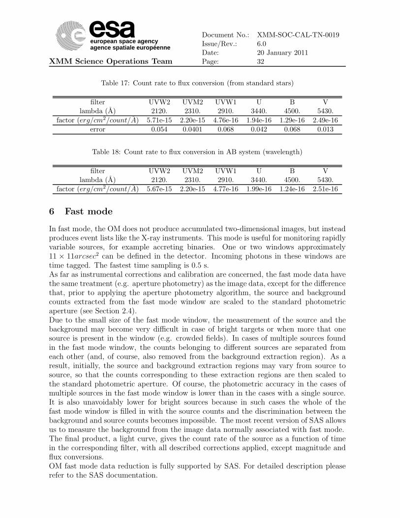
If we take the standard flux at the effective wavelengths of the OM filters (see Table15) and their measured count rates, including time sensitivity degradation correction (seeTable 16), we can derive a direct count rate to flux conversion factor. After dividing andaveraging we obtain the results of Table 17. (Quoted relative errors are computed asstdev/mean).The difference between these factors and the ones obtained from simulations are less than1 %, an expected result since the simulator is based in the same stars.We obtained (see Table 13) flux conversion factors in the AB system. Even if we arein frequency space, we can characterize the filter by its effective wavelength. And thenwe can convert these factors to lambda space by multiplying by (c/λ2 ). The results areshown in Table 18.




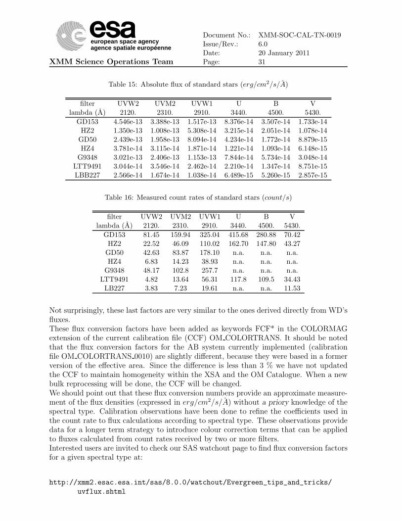
Table 15: Absolute flux of standard stars (erg/cm2/s/A)


GD153 4.546e-13 3.388e-13 1.517e-13 8.376e-14 3.507e-14 1.733e-14HZ2 1.350e-13 1.008e-13 5.308e-14 3.215e-14 2.051e-14 1.078e-14

GD50 2.439e-13 1.958e-13 8.094e-14 4.234e-14 1.772e-14 8.879e-15HZ4 3.781e-14 3.115e-14 1.871e-14 1.221e-14 1.093e-14 6.148e-15

G9348 3.021e-13 2.406e-13 1.153e-13 7.844e-14 5.734e-14 3.048e-14LTT9491 3.044e-14 3.546e-14 2.462e-14 2.210e-14 1.347e-14 8.751e-15LBB227 2.566e-14 1.674e-14 1.038e-14 6.489e-15 5.260e-15 2.857e-15

Table 16: Measured count rates of standard stars (count/s)


GD153 81.45 159.94 325.04 415.68 280.88 70.42HZ2 22.52 46.09 110.02 162.70 147.80 43.27

GD50 42.63 83.87 178.10 n.a. n.a. n.a.HZ4 6.83 14.23 38.93 n.a. n.a. n.a.

G9348 48.17 102.8 257.7 n.a. n.a. n.a.LTT9491 4.82 13.64 56.31 117.8 109.5 34.43LB227 3.83 7.23 19.61 n.a. n.a. 11.53

Not surprisingly, these last factors are very similar to the ones derived directly from WD’sfluxes.These flux conversion factors have been added as keywords FCF* in the COLORMAGextension of the current calibration file (CCF) OM COLORTRANS. It should be notedthat the flux conversion factors for the AB system currently implemented (calibrationfile OM COLORTRANS 0010) are slightly different, because they were based in a formerversion of the effective area. Since the difference is less than 3 % we have not updatedthe CCF to maintain homogeneity within the XSA and the OM Catalogue. When a newbulk reprocessing will be done, the CCF will be changed.We should point out that these flux conversion numbers provide an approximate measure-ment of the flux densities (expressed in erg/cm2/s/A) without a priory knowledge of thespectral type. Calibration observations have been done to refine the coefficients used inthe count rate to flux calculations according to spectral type. These observations providedata for a longer term strategy to introduce colour correction terms that can be appliedto fluxes calculated from count rates received by two or more filters.Interested users are invited to check our SAS watchout page to find flux conversion factorsfor a given spectral type at:

http://xmm2.esac.esa.int/sas/8.0.0/watchout/Evergreen_tips_and_tricks/

uvflux.shtml




Table 17: Count rate to flux conversion (from standard stars)



error 0.054 0.0401 0.068 0.042 0.068 0.013

Table 18: Count rate to flux conversion in AB system (wavelength)



6 Fast mode

In fast mode, the OM does not produce accumulated two-dimensional images, but insteadproduces event lists like the X-ray instruments. This mode is useful for monitoring rapidlyvariable sources, for example accreting binaries. One or two windows approximately11 × 11arcsec2 can be defined in the detector. Incoming photons in these windows aretime tagged. The fastest time sampling is 0.5 s.As far as instrumental corrections and calibration are concerned, the fast mode data havethe same treatment (e.g. aperture photometry) as the image data, except for the differencethat, prior to applying the aperture photometry algorithm, the source and backgroundcounts extracted from the fast mode window are scaled to the standard photometricaperture (see Section 2.4).Due to the small size of the fast mode window, the measurement of the source and thebackground may become very difficult in case of bright targets or when more that onesource is present in the window (e.g. crowded fields). In cases of multiple sources foundin the fast mode window, the counts belonging to different sources are separated fromeach other (and, of course, also removed from the background extraction region). As aresult, initially, the source and background extraction regions may vary from source tosource, so that the counts corresponding to these extraction regions are then scaled tothe standard photometric aperture. Of course, the photometric accuracy in the cases ofmultiple sources in the fast mode window is lower than in the cases with a single source.It is also unavoidably lower for bright sources because in such cases the whole of thefast mode window is filled in with the source counts and the discrimination between thebackground and source counts becomes impossible. The most recent version of SAS allowsus to measure the background from the image data normally associated with fast mode.The final product, a light curve, gives the count rate of the source as a function of timein the corresponding filter, with all described corrections applied, except magnitude andflux conversions.OM fast mode data reduction is fully supported by SAS. For detailed description pleaserefer to the SAS documentation.




7 OM Grisms

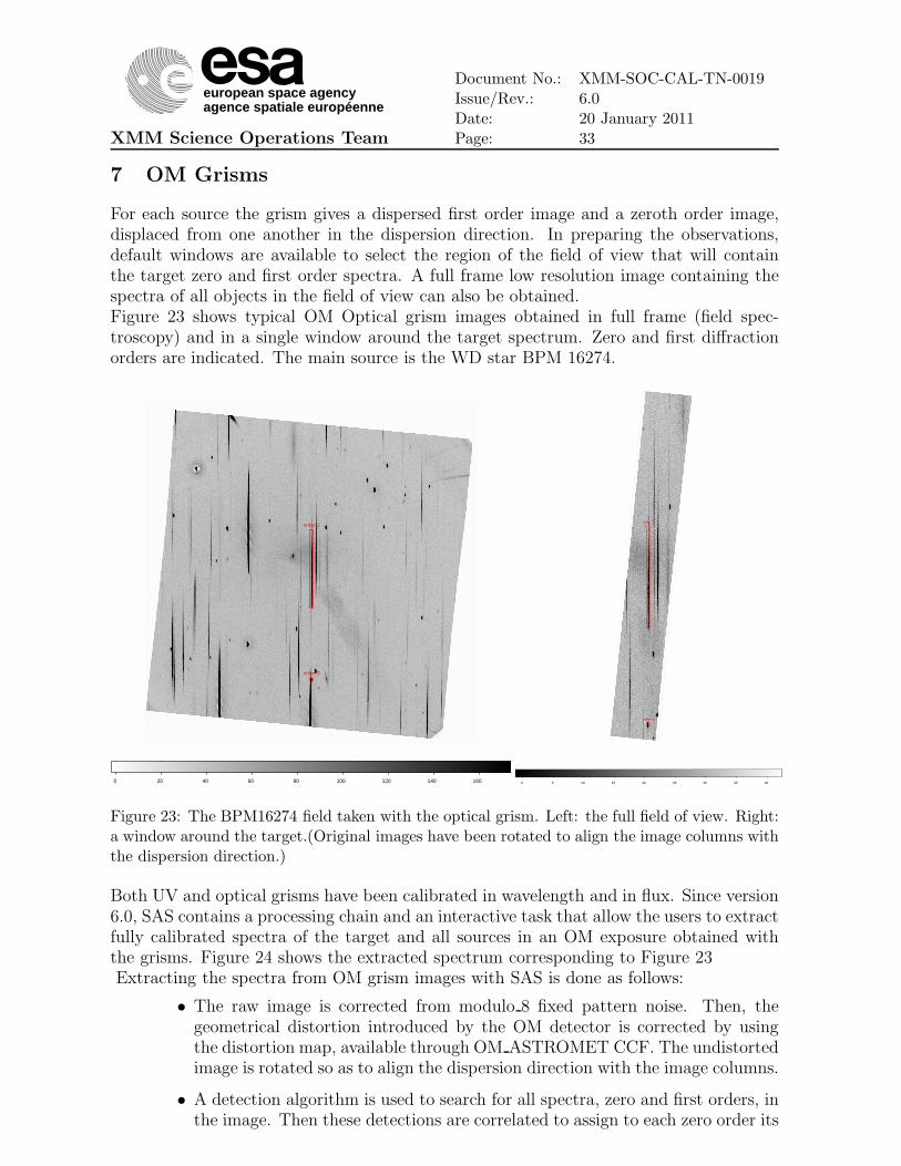
For each source the grism gives a dispersed first order image and a zeroth order image,displaced from one another in the dispersion direction. In preparing the observations,default windows are available to select the region of the field of view that will containthe target zero and first order spectra. A full frame low resolution image containing thespectra of all objects in the field of view can also be obtained.Figure 23 shows typical OM Optical grism images obtained in full frame (field spec-troscopy) and in a single window around the target spectrum. Zero and first diffractionorders are indicated. The main source is the WD star BPM 16274.

0 20 40 60 80 100 120 140 160

order 1

order 0

0 5 10 15 20 25 30 35 40

order 1

order 0

Figure 23: The BPM16274 field taken with the optical grism. Left: the full field of view. Right:a window around the target.(Original images have been rotated to align the image columns withthe dispersion direction.)

Both UV and optical grisms have been calibrated in wavelength and in flux. Since version6.0, SAS contains a processing chain and an interactive task that allow the users to extractfully calibrated spectra of the target and all sources in an OM exposure obtained withthe grisms. Figure 24 shows the extracted spectrum corresponding to Figure 23Extracting the spectra from OM grism images with SAS is done as follows:

• The raw image is corrected from modulo 8 fixed pattern noise. Then, thegeometrical distortion introduced by the OM detector is corrected by usingthe distortion map, available through OM ASTROMET CCF. The undistortedimage is rotated so as to align the dispersion direction with the image columns.

• A detection algorithm is used to search for all spectra, zero and first orders, inthe image. Then these detections are correlated to assign to each zero order its




Figure 24: The BPM16274 spectrum taken with the optical grism. Left: raw spectrum. Right:flux calibrated spectrum. Hydrogen Balmer lines are clear.

corresponding first order. Spectral extraction is performed on the successfulcases.

• The positions of the zero orders of the extracted spectra are used to derive theastronomical coordinates of the corresponding sources. This is particularlyuseful in case of field spectroscopy when OM is used in full frame mode withthe grisms. Matching the positions of the zero orders with their correspondingpositions in a direct image requires an additional distortion map for each grism.(See Section 2.7.)

• The extracted spectra are calibrated in wavelength and in absolute flux.

As we have said before, the reader is referred to the SAS documentation for details onthe complete grism data reduction.

7.1 Wavelength calibration

The dispersion relations have been obtained by observing several F type stars for theUV grism, and a DA2 white dwarf (BPM 16274) for the Visible grism. The wavelengthscales are provided as a function of the distance (X) in pixels (at full resolution) from thecentroid of the zeroth order in the extracted spectrumFor the Visible grism, we have

λ(A) = 5.626 × X + 200.898 ± 7.5 (22)

and for the UV grism,

λ(A) = 0.000771 × X2 + 1.866 × X + 991.778 ± 2.0 (23)

Uncertainties in measuring the position of the zeroth order may produce a shift in thescale of ± 10 A for the UV grism and ± 20 A for the visible grism.

The applied fixed pattern modulo 8 noise correction is not perfect, particularly for thevisible grism. This effect limits the spectral resolution of the OM grisms, which is better




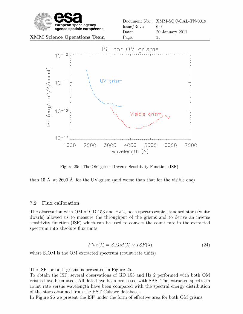
Figure 25: The OM grisms Inverse Sensitivity Function (ISF)

than 15 A at 2600 A for the UV grism (and worse than that for the visible one).

7.2 Flux calibration

The observation with OM of GD 153 and Hz 2, both spectroscopic standard stars (whitedwarfs) allowed us to measure the throughput of the grisms and to derive an inversesensitivity function (ISF) which can be used to convert the count rate in the extractedspectrum into absolute flux units

F lux(λ) = S OM(λ) × ISF (λ) (24)

where S OM is the OM extracted spectrum (count rate units)

The ISF for both grisms is presented in Figure 25.To obtain the ISF, several observations of GD 153 and Hz 2 performed with both OMgrisms have been used. All data have been processed with SAS. The extracted spectra incount rate versus wavelength have been compared with the spectral energy distributionof the stars obtained from the HST Calspec database.In Figure 26 we present the ISF under the form of effective area for both OM grisms.




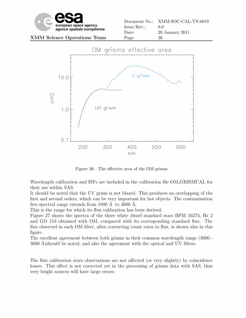
Figure 26: The effective area of the OM grisms

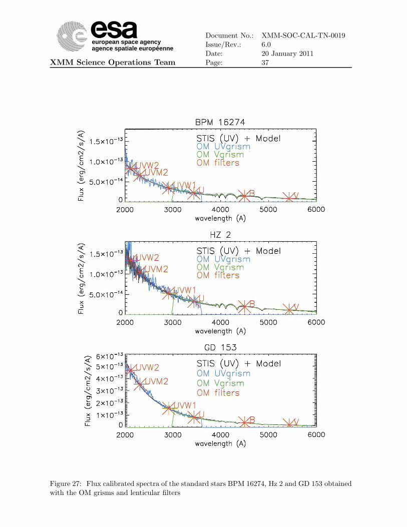
Wavelength calibration and ISFs are included in the calibration file OM GRISMCAL fortheir use within SAS.It should be noted that the UV grism is not blazed. This produces an overlapping of thefirst and second orders, which can be very important for hot objects. The contaminationfree spectral range extends from 1800 A to 3600 A.This is the range for which its flux calibration has been derived.Figure 27 shows the spectra of the three white dwarf standard stars BPM 16274, Hz 2and GD 153 obtained with OM, compared with its corresponding standard flux. Theflux observed in each OM filter, after converting count rates to flux, is shown also in thisfigure.The excellent agreement between both grisms in their common wavelength range (3000 -3600 A)should be noted, and also the agreement with the optical and UV filters.

The flux calibration stars observations are not affected (or very slightly) by coincidencelosses. This effect is not corrected yet in the processing of grisms data with SAS, thusvery bright sources will have large errors.




Figure 27: Flux calibrated spectra of the standard stars BPM 16274, Hz 2 and GD 153 obtainedwith the OM grisms and lenticular filters




8 Current Calibration Files (CCFs) for SAS

Table 19 provides a list of the OM calibration files. The SAS tasks using a given CCFare indicated as well. For a detailed description of these files and of their usage, theuser is referred to the CCF interface document and to the Calibration Access and DataHandbook

http://xmm2.esac.esa.int/external/xmm_sw_cal/calib/documentation/CALHB/index.html

Table 19: Calibration files of the Optical Monitor.

File name File Content SAS task

ASTROMET coefficients for geometric distortion cor-rection

omatt omde-tect om-drifthistomgprep

BADPIX bad pixels position, type of defect and theseverity level

omcosflag om-fastflat

BORESIGHT alignment of the instruments and startracker

omatt omg-prep

COLORTRANS zero points, coefficients for color transfor-mation into a standard system count rateto flux conversion

ommag omde-tect omlcbuild

GRISMCAL wavelength and flux calibrations for thegrisms

omgrism

HKPARMINT house keeping parameter ranges ommagLARGESCALESENS flat field map (set to unity) omflatgenPHOTTONAT correction coefficients of count rates for

detector non-linearity and agingommag om-prep omdetectomlcbuild

PIXTOPIXSENS flat field map (set to unity) omflatgenPSF1DRB point spread function for each filter ommag omde-

tect omlcbuild

9 Future calibration plans

Most of the calibration items have been covered in this description. All of them have beenincorporated into the standard data reduction done with SAS.A few refinements and some new developments are on the way. Among them:

• Search and characterisation of very large scale sensitivity variations

• Better treatment of fast mode photometry

• Revision of standard colour transformations




• UV colour transformations derived from observations (XSA and OM Cata-logue) instead of simulations

• Time dependent sensitivity variations in the grisms

• Wavelength calibration variation in the UV grism across the detector

• New assessment of errors

10 Acknowledgments

We thank all the people who have contributed to the operation and calibration of XMM-OM. This includes many people at MSSL (Alice Breeveld, Cynthia James, Tracey Poole,Elizabeth Auden, Keith Mason, Simon Rosen, Chris Brindle, Vladimir Yersow, Mat Page,Martin Still), Liege University (Igor Antokhin), UCSB (Tim Sasseen, Bob Shirey, JamieKennea), ESTEC (Rudi Much) and ESAC (Nora Loiseau, Eva Verdugo, Marıa Diaz,Bing Chen, Jan Uwe Ness, Antonio Talavera). We thank also the Mission Planning andMission Operations Teams at ESAC and ESOC. Without them the whole mission wouldnot operate every day and no calibration would be possible. Finally we thank Marıa deSantos for her careful reading and useful comments to this document.

11 References

Antokhin I., Breeveld A., Chen B., et al. 2002, ESA SP-488, Proc. Symposium ’New

Visions of the X-ray Universe in the X MM-Newton and Chandra Era’

Antokhin I., 2002, Internal Report to the OM Calibration Team.Breeveld A.A., Curran P.A., Hoversten E.A. et al, 2010, MNRAS, 406, 1687Colina L., Bohlin R.C., 1994, AJ, 108, 1931Gunn J.E., Stryker L.L., 1983, ApJ Supplement, 51, 121Kirsch M.G. et al, 2005, Proc. SPIE, Vol 5898, 212Landolt A. U., 1992, AJ, 104, 340Mason K.O., Breeveld A.A., Much R.M. et al. 2001, A&A 365, L36Mason K.O., 2002, ESA SP-488, ESTEC, The NetherlandsOke J.B., ApJS, 27, 21Poole T.S., 2006, MSSL Internal ReportStetson P. B., 2000, PASP, 112, 925




12 Appendix A: Calibration stars

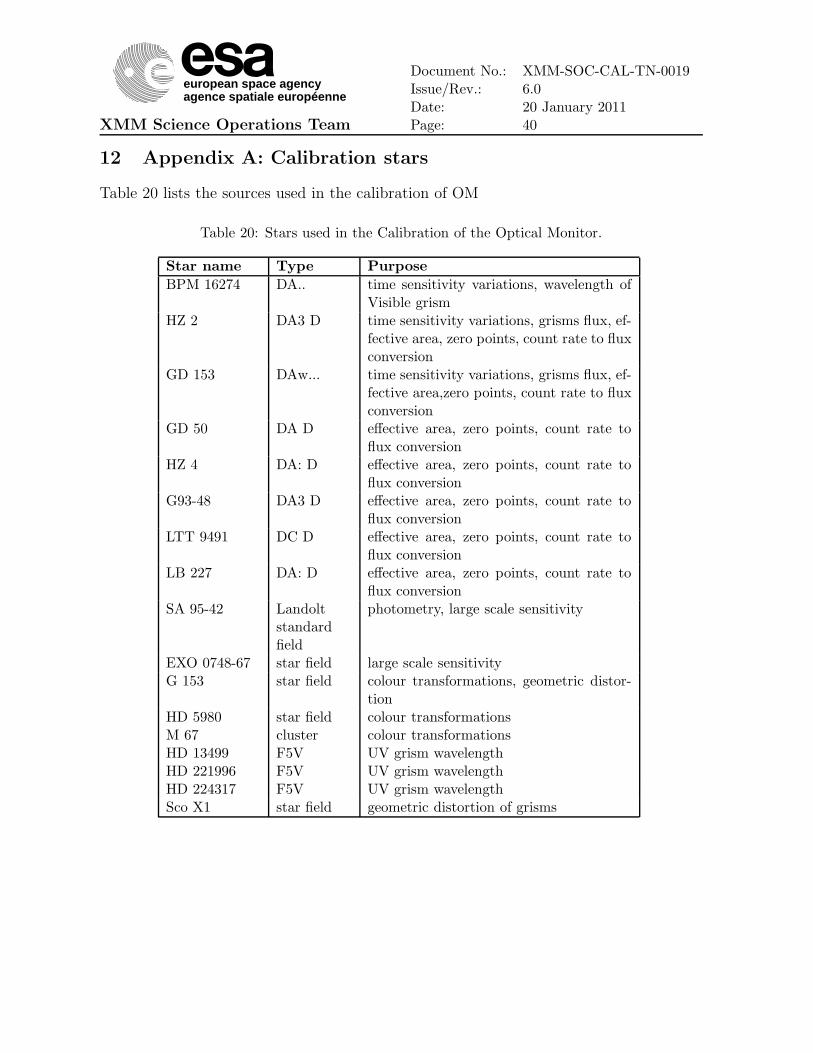
Table 20 lists the sources used in the calibration of OM

Table 20: Stars used in the Calibration of the Optical Monitor.

Star name Type Purpose

BPM 16274 DA.. time sensitivity variations, wavelength ofVisible grism

HZ 2 DA3 D time sensitivity variations, grisms flux, ef-fective area, zero points, count rate to fluxconversion

GD 153 DAw... time sensitivity variations, grisms flux, ef-fective area,zero points, count rate to fluxconversion

GD 50 DA D effective area, zero points, count rate toflux conversion

HZ 4 DA: D effective area, zero points, count rate toflux conversion

G93-48 DA3 D effective area, zero points, count rate toflux conversion

LTT 9491 DC D effective area, zero points, count rate toflux conversion

LB 227 DA: D effective area, zero points, count rate toflux conversion

SA 95-42 Landoltstandardfield

photometry, large scale sensitivity

EXO 0748-67 star field large scale sensitivityG 153 star field colour transformations, geometric distor-

tionHD 5980 star field colour transformationsM 67 cluster colour transformationsHD 13499 F5V UV grism wavelengthHD 221996 F5V UV grism wavelengthHD 224317 F5V UV grism wavelengthSco X1 star field geometric distortion of grisms




13 Appendix B: Summary of errors and repeatability

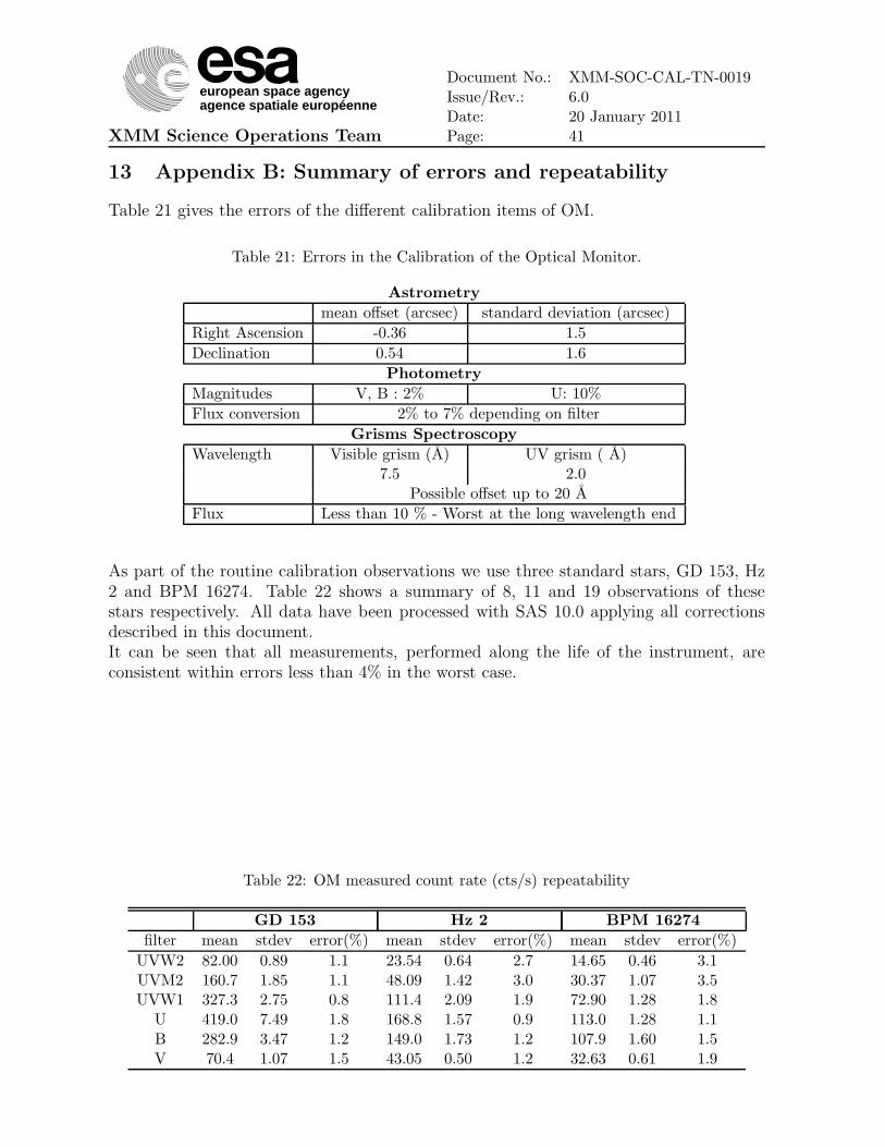
Table 21 gives the errors of the different calibration items of OM.

Table 21: Errors in the Calibration of the Optical Monitor.

Astrometry

mean offset (arcsec) standard deviation (arcsec)

Right Ascension -0.36 1.5

Declination 0.54 1.6

Photometry

Magnitudes V, B : 2% U: 10%

Flux conversion 2% to 7% depending on filter

Grisms Spectroscopy

Wavelength Visible grism (A) UV grism ( A)7.5 2.0

Possible offset up to 20 A

Flux Less than 10 % - Worst at the long wavelength end

As part of the routine calibration observations we use three standard stars, GD 153, Hz2 and BPM 16274. Table 22 shows a summary of 8, 11 and 19 observations of thesestars respectively. All data have been processed with SAS 10.0 applying all correctionsdescribed in this document.It can be seen that all measurements, performed along the life of the instrument, areconsistent within errors less than 4% in the worst case.

Table 22: OM measured count rate (cts/s) repeatability

GD 153 Hz 2 BPM 16274

filter mean stdev error(%) mean stdev error(%) mean stdev error(%)

UVW2 82.00 0.89 1.1 23.54 0.64 2.7 14.65 0.46 3.1UVM2 160.7 1.85 1.1 48.09 1.42 3.0 30.37 1.07 3.5UVW1 327.3 2.75 0.8 111.4 2.09 1.9 72.90 1.28 1.8

U 419.0 7.49 1.8 168.8 1.57 0.9 113.0 1.28 1.1B 282.9 3.47 1.2 149.0 1.73 1.2 107.9 1.60 1.5V 70.4 1.07 1.5 43.05 0.50 1.2 32.63 0.61 1.9

XMM-Newton Optical and UV Monitor (OM) Calibration...

Documents

Transcript of XMM-Newton Optical and UV Monitor (OM) Calibration...