
T r r f x x x x f x x x T r T r r a a a x n f x x a x a x ...

if y = loga x then x = a y
x log b x = b
loga a = 1
loga a x( ) = x
a log a x = x
loga M ⋅ N( ) = loga M + loga N
loga Mp( ) = P ⋅ loga M
loga
MN
= loga M − loga N
a
M
N
= an
M
a−N =
1aN
Sx = x − a + bi( )[ ]⋅ x − a − bi( )[ ] = x2 − 2ax + a2 + b2( )
cos2 x + sin2 x = 1
sin 2( ) = 2sin( )⋅ cos( )
cos 2( ) = cos2 − sin2 cos 2( ) = 1 − 2sin2cos 2( ) = 2cos2 −1
sin
2
= ±
1 − cos2
cos2
= ±
1 + cos2
tan 2( ) =2 t a n
1− tan 2
tan
2
=
1 − cossin
=sin
1 + cos
loga x =
ln xln a
sin + sin = 2 sin
+2
cos−2
sin − sin = 2 cos
+2
sin−2
cos + cos = 2 cos
+2
cos−2
cos − cos = 2 sin
+2
sin−2
sin +( ) = sin cos + cos sin sin −( ) = sin cos − cos sin
cos +( ) = cos cos − sin sincos −( ) = cos cos + sin sin
ax 2 + bx + c = 0
x =−b ± b 2 − 4ac
2a
Page 1
Math Reference Trigonometry & Analysis James Lamberg
cos π2
+ x
= − sin x
cos π2
− x
= sin x
cos π ± x( ) = − cos x
cos3π2
+ x
= sin x
cos3π2
− x
= − sin x
sinπ2
± x
= cos x
sin π + x( ) = − sin x
sin π − x( ) = sin x
sin 3π2
± x
= − cos x
tanπ2
+ x
= − cot x
tanπ2
− x
= cot x
tan π + x( ) = tan x
tan π − x( ) = − tan x
tan 3π2
+ x
= − cot x
tan 3π2
− x
= cot x
∀ for every
∈ element of
∃ there exists
∋ such that
∴ therefore
Q since
¬ not
∧ and
∨ or
d derive
integrate∫x=a evaluate with x = a
∝ proportional to
p precedes
f follows
≅ congruent to
∪ union
∩ intersection
⊆ subset
⊇ superset
⊂ proper subset
⊃ propor superset
C (fancy) compliment
⇒ implies
⇔ double implication
~ negation or ¬( )Q.E.D: Quod Erat Demonstandum
"that which was to be proved"
tan −( ) =tan − tan
1 + tan tan
tan +( ) =tan + tan
1 − tan tan
Mid =x2 − x1
2,
y2 − y1
2
Dist = x2 − x1( )2+ y2 − y1( )2
A =
12r2 , sector area

c2 = a2 + b2 − 2ab cos
b2 = a2 + c2 − 2ac cosa2 = b2 + c2 − 2bc cos
sina
=sinb
=sinc
K =
12bc sin
y = A ⋅ sin x -( ) + K, > 0
Amplitude = A =
M − m2
Period =
2π
Phase Shift =
Frequency =
1period
=2π
Critical Points =
period4
Unit Circle
cos, sin( ) 0,0° = 1, 0( )
π6, 3 0° =
32,12
π4, 4 5° =
22,
22
π3, 6 0° =
12,
32
π2, 9 0° = 0,1( )
2π3,120 ° = −
12,
32
3π4,135° = −
22,
22
5π6,150 ° = −
32,12
π,180° = −1,0( )
7π6,210° = −
32,−
12
5π4,225° = −
22,−
22
4π3,240° = −
12, −
32
3π4,270° = 0, −1( )
5π3,300° =
12,−
32
11π6
,330° =32, −
12
Page 2
\Math Reference Trigonometry & Analysis James Lamberg
ab = a ⋅ b a 2 = a a
b=
a
ban = a
n
if a < b & b < c, then a < c
if a < b & c < d, then a + c < b + d
if a < b then a + k < b + k
if a < b & k > 0, then ak < bk
if a < b & k < 0, then ak > bk
a + b ≤ a + b
¯ a ≤ a ≤ a a ≤ k iff ¯k ≤ a ≤ k
a ≥ k iff a ≤ -k of a ≥ k
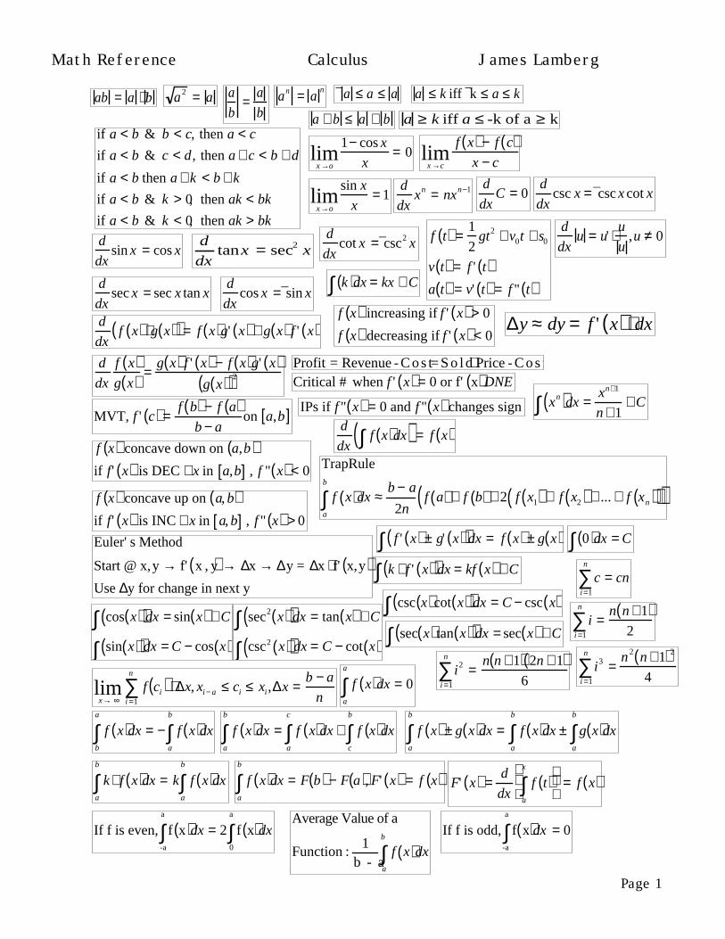
x→olim
sin x
x= 1
x →olim
1− cos x
x= 0
x →clim
f x( ) − f c( )x − c
d
dxxn = nxn−1 d
dxC = 0
d
dxtanx = sec2 x
d
dxsin x = cos x
d
dxcos x =¯sin x
d
dxcot x =¯csc2 x
d
dxsec x = sec x tan x
f t( ) =1
2gt2 + v0t + s0
v t( ) = f ' t( )a t( ) = v' t( ) = f " t( )
d
dxcsc x = ¯csc x cot x
d
dxf x( )⋅ g x( )( ) = f x( )g' x( ) + g x( ) f ' x( )
d
dxu = u' ⋅
u
u,u ≠ 0
Profit = Revenue - C o s t= S o l d⋅ Price - C o s tCritical # when f ' x( ) = 0 or f' x( )DNE
f x( ) increasing if f ' x( ) > 0
f x( ) decreasing if f ' x( ) < 0
MVT, f ' c( ) =f b( ) − f a( )
b − aon a,b[ ] IPs if f " x( ) = 0 and f " x( ) changes sign
∆y ≈ dy = f ' x( ) ⋅ dx
f x( ) concave down on a,b( ) if f ' x( ) is DEC ∀x in a,b[ ] , f " x( ) < 0
f x( ) concave up on a, b( ) if f ' x( ) is INC ∀x in a, b[ ] , f " x( ) > 0
d
dxf x( )dx∫( ) = f x( )
k( )∫ dx = kx + C
xn( )∫ dx =xn+1
n +1+ C
TrapRule
f x( )dx ≈b − a
2na
b
∫ f a( ) + f b( ) + 2 f x1( ) + f x2( ) + ... + f xn( )( )( )
Euler' s Method
Start @ x,y → f' x , y( ) → ∆x → ∆y = ∆x ⋅ f' x,y( )Use ∆y for change in next y
k ⋅ f ' x( )( )∫ dx = kf x( ) + C
f ' x( ) ± g' x( )( )∫ dx = f x( ) ± g x( ) 0( )∫ dx = C
sec2 x( )( )∫ dx = tan x( ) + C
csc2 x( )( )∫ dx = C − cot x( )sec x( ) tan x( )( )∫ dx = sec x( ) + C
csc x( )cot x( )( )∫ dx = C − csc x( )c
i=1
n
∑ = cn
ii =1
n
∑ =n n + 1( )
2
i2
i =1
n
∑ =n n +1( ) 2n + 1( )
6i3
i =1
n
∑ =n 2 n + 1( )2
4
cos x( )( )∫ dx = sin x( ) + C
sin x( )( )∫ dx = C − cos x( )
x→ ∞lim f ci( )
i =1
n
∑ ⋅ ∆x, xi− a ≤ ci ≤ xi,∆x =b − a
nf x( )dx
a
a
∫ = 0
f x( )b
a
∫ dx = − f x( )a
b
∫ dx f x( )a
b
∫ dx = f x( )a
c
∫ dx + f x( )c
b
∫ dx
k ⋅ f x( )a
b
∫ dx = k f x( )a
b
∫ dx
f x( ) ± g x( )a
b
∫ dx = f x( )a
b
∫ dx ± g x( )a
b
∫ dx
f x( )a
b
∫ dx = F b( ) − F a( ), F' x( ) = f x( ) F' x( ) =d
dxf t( )
a
x
∫
= f x( )
If f is even, f x( )-a
a
∫ dx = 2 f x( )0
a
∫ dxAverage Value of a
Function :1
b - af x( )dx
a
b
∫If f is odd, f x( )
-a
a
∫ dx = 0
d
dx
f x( )g x( ) =
g x( ) f ' x( ) − f x( )g' x( )g x( )( )2
Math Reference Calculus James Lamberg
Page 1

ln x( ) =1
tdt, x > 0
1
x
∫ln 1( ) = 0 ln a ⋅ b( ) = ln a( ) + ln b( )
lna
b
= ln a( ) − ln b( )
ln a( ) n = n ⋅ ln a( )
ln e( ) =1
tdt = 1
1
e
∫ln ex( ) = x
d
dxln u( ) =
d
dxln u =
du
u
1
udu = ln u( ) + C∫
tan x( )dx = C − ln cos x( )∫ = l n secx( ) + C
cot x( )dx = l n s inx( ) + C∫ = C − l ncscx( ) sec x( )dx = ln sec x( ) + tan x( ) + C∫csc x( )dx = C − ln csc x( ) + cot x( )∫f −1 x( ) = g x( ),g' x( ) =
1
g' g x( )( )f −1 x( ) = g x( ), a,b( ) f , g' b( ) =
1
f ' a( )
ea ⋅ eb = ea+ b
ea
eb= ea− b
d
dxeu( )du = eu ⋅du
loga x( ) =ln x( )ln a( )
d
dxa u( ) = ln a( ) ⋅ au ⋅du
d
dxloga u( )( ) =
du
ln a( )⋅ u
ax( )dx =ax
ln a( )∫ + Cd
dxu n( ) = n ⋅u n −1( ) ⋅ du
d
dxee( ) = 0
d
dxx x( ) = ln x( ) +1( )⋅ x x
e = limx→∞
1 +1
x
x
Compounded n times a year
A = P 1+ r
n
n⋅t
Compounded Continously
A = P ⋅ er⋅t Newton' s Law of Cooling
dT
dt= k To − Ts( )
y = arcsin x( ), iff sin y( ) = x
y = arccos x( ), iff cos y( ) = x
y = arctan x( ), iff tan y( ) = x
y = arccot x( ), iff cot y( ) = x
y = arcsec x( ), iff sec y( ) = x
y = arccsc x( ), iff csc y( ) = x
y = arcsin x( ),D : -1,1[ ], R : − π2
,π2
y = arccos x( ), D: -1,1[ ],R : 0,π[ ]
y = arctan x( ), D: -∞,∞( ),R : −π2
,π2
y = arccot x( ), D :-∞, ∞( ), R : 0, π( )y = arcsec x( ), D :x ≥1( ), R : 0,π( )
y = arccsc x( ), D :x ≥ 1( ),R : − π2
,π2
eπi +1 = 0
d
dxarcsin u( )( ) =
1
1− u 2⋅ du
d
dxarccos u( )( ) =
−1
1 − u2⋅ du
d
dxarctan u( )( ) =
1
1 + u2⋅du
d
dxarc cot u( )( ) =
−1
1 + u2⋅ du
d
dxarc sec u( )( ) =
1
u u2 −1⋅ du
d
dxarc csc u( )( ) =
−1
u u2 −1⋅ du
du
a2 − u 2∫ = arcsinu
a
+ C
du
a2 + u 2∫ =1
aarctan
u
a
+ C
du
u u2 − a 2∫ =1
aarcsec
u
a+ C
cosh2 x − sinh2 x = 1
tanh 2 x + sec h 2x = 1
coth 2 x − csch 2x = 1
sinh 2x( ) = 2 sinh x( )⋅ cosh x( )
cosh 2x( ) = cosh 2 x ⋅sinh2 x
sinh2 x =cosh 2x( ) −1
2
cosh2 x =cosh 2x( ) + 1
2sinh x + y( ) = sinh x( )⋅ cosh y( ) + cosh x( )⋅ sinh y( )sinh x − y( ) = sinh x( )⋅ cosh y( ) − cosh x( )⋅ sinh y( )cosh x + y( ) = cosh x( ) ⋅cosh y( ) + sinh x( ) ⋅sinh y( )cosh x − y( ) = cosh x( ) ⋅cosh y( ) − sinh x( ) ⋅sinh y( )
sinh x( ) = ex − e− x
2
cosh x( ) =e x + e−x
2
cosh u( )∫ ⋅ du = sinh u( ) + C
sinh u( )⋅∫ du = cosh u( ) + C
sec h2u∫ ⋅ du = tanh u( ) + C
csc h2u∫ ⋅ du = C − coth u( )
sec h u( ) ⋅ tanh u( )∫ ⋅ du = C − sec h u( )
csc h u( ) ⋅ coth u( )∫ ⋅ du = C − csc h u( )
d
dxsinh u( ) = cosh u( ) ⋅ du
d
dxcosh u( ) = sinh u( ) ⋅ du
d
dxtanh u( ) = sech 2u ⋅du
d
dxcoth u( ) = −csc h2u ⋅ du
d
dxsec h u( ) = − sec h u( ) ⋅ tanh u( )( ) ⋅ du
d
dxcsc h u( ) = − csch u( )⋅ coth u( )( )⋅ du
Page 2
Math Reference Calculus James Lamberg
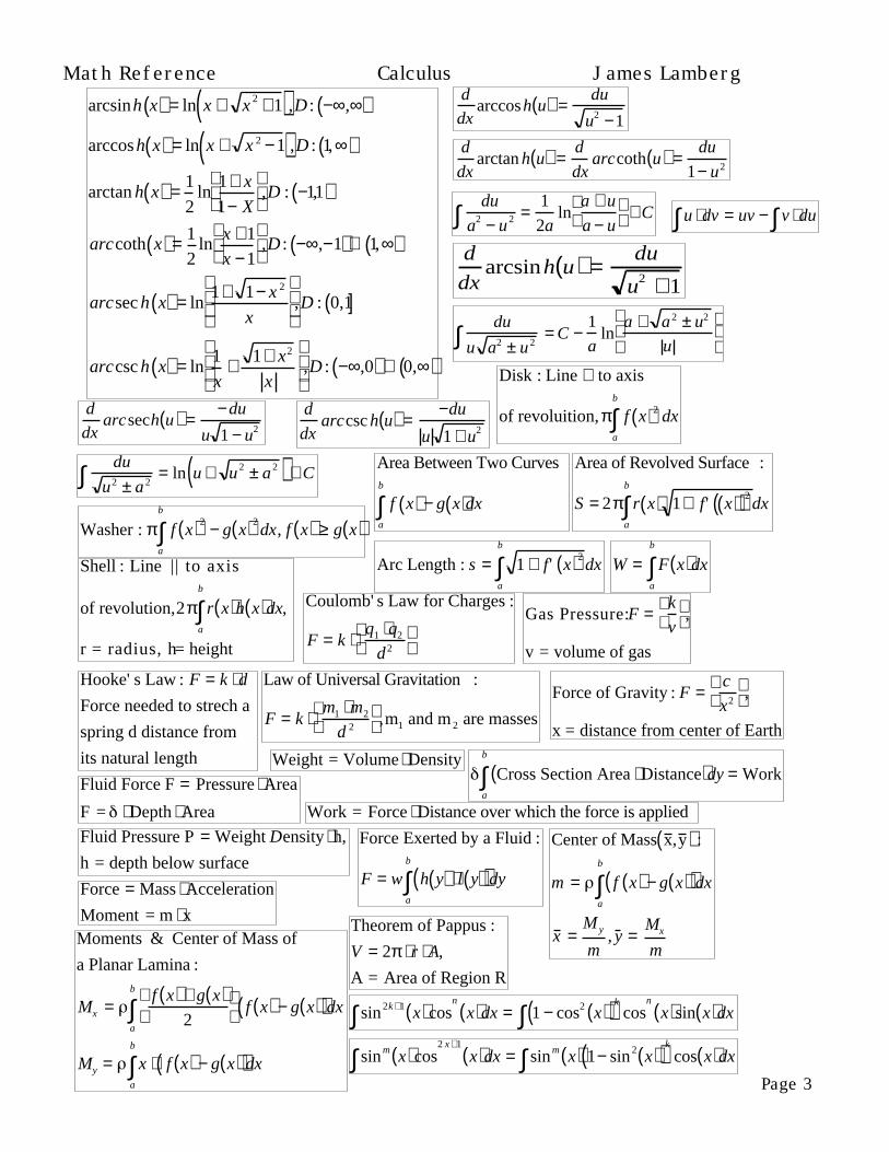
arcsinh x( ) = ln x + x 2 +1( ),D : −∞,∞( )
arccosh x( ) = ln x + x 2 −1( ),D : 1,∞( )
arctan h x( ) = 1
2ln
1+ x
1− X
,D : −1,1( )
arccoth x( ) = 1
2ln
x +1
x −1
,D : −∞,−1( )∪ 1,∞( )
arcsec h x( ) = ln1+ 1− x 2
x
,D : 0,1( ]
arccsc h x( ) = ln1
x+ 1+ x2
x
,D : −∞,0( ) ∪ 0,∞( )
d
dxarcsinh u( ) =
du
u2 +1
d
dxarccosh u( ) =
du
u2 −1
d
dxarctan h u( ) =
d
dxarccoth u( ) =
du
1− u2
d
dxarcsech u( ) =
−du
u 1 − u2
d
dxarccsc h u( ) =
−du
u 1 + u2
du
u2 ± a2∫ = ln u + u2 ± a2( ) + C
du
a2 − u 2∫ =1
2aln
a + u
a − u
+ C
du
u a2 ± u2∫ = C −1
aln
a + a2 ± u2
u
Area Between Two Curves
f x( ) − g x( )a
b
∫ dx
Disk : Line ⊥ to axis
of revoluition,π f x( )2 dxa
b
∫
Washer : π f x( )2
a
b
∫ − g x( )2dx, f x( ) ≥ g x( )
Shell : Line | | to axis
of revolution,2π r x( )h x( )dx,a
b
∫
r = radius, h= height
Arc Length : s = 1 + f ' x( )2dx
a
b
∫
Area of Revolved Surface :
S = 2π r x( ) 1+ f ' x( )( )2dx
a
b
∫
Work = Force ⋅ Distance over which the force is applied
W = F x( )dxa
b
∫
Hooke' s Law : F = k ⋅ d
Force needed to strech a
spring d distance from
its natural length
Law of Universal Gravitation :
F = k ⋅m1 ⋅ m2
d 2
,m1 and m 2 are masses
Coulomb' s Law for Charges :
F = k ⋅q1 ⋅q2
d2
Force of Gravity : F =c
x2
,
x = distance from center of Earth
Gas Pressure:F =k
v
,
v = volume of gas
Weight = Volume ⋅ DensityCross Section Area ⋅ Distance( )dy = Work
a
b
∫Fluid Force F = Pressure ⋅ Area
F = ⋅ Depth ⋅ Area
Fluid Pressure P = Weight Density ⋅ h,
h = depth below surface
Force Exerted by a Fluid :
F = w h y( ) ⋅ l y( )( )dya
b
∫Force = Mass ⋅ Acceleration
Moment = m ⋅ xMoments & Center of Mass of
a Planar Lamina :
Mx =f x( ) + g x( )
2
a
b
∫ f x( ) − g x( )( )dx
My = x ⋅ f x( ) − g x( )( )a
b
∫ dx
Center of Mass x ,y ( ) :
m = f x( ) − g x( )( )dxa
b
∫
x =M y
m, y =
Mx
m
Theorem of Pappus :
V = 2π ⋅ r ⋅ A,
A = Area of Region R
u ⋅ dv = uv − v ⋅ du∫∫
sin 2k +1 x( )cos∫n
x( )dx = 1 − cos2 x( )( )kcos∫
n
x( )sin x( )dx
sinm x( )cos∫2 x +1
x( )dx = sinm x( ) 1− sin 2 x( )( )∫k
cos x( )dx
Page 3
Math Reference Calculus James Lamberg
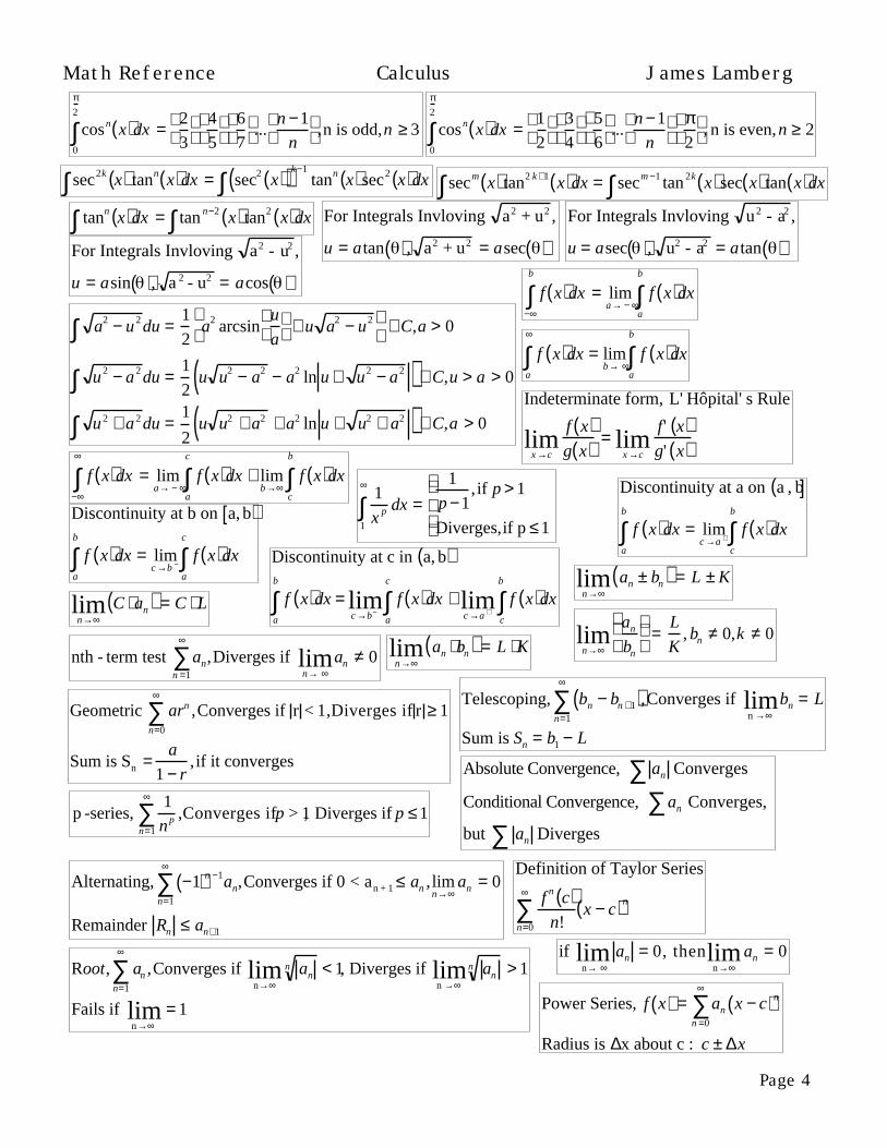
cosn x( )dx =2
3
4
5
6
7
...
n −1
n
,n is odd,n ≥ 3
0
π2
∫ cosn x( )dx =1
2
3
4
5
6
...
n −1
n
π2
, n is even,n ≥ 2
0
π2
∫
sec2k x( ) tann x( )dx∫ = sec2 x( )( )k−1tann x( )sec2 x( )dx∫ secm x( ) tan2 k +1 x( )dx∫ = secm −1 tan 2k x( )sec x( ) tan x( )dx∫
tann x( )dx∫ = tan n−2 x( ) tan2 x( )dx∫For Integrals Invloving a2 - u2 ,
u = asin( ), a 2 - u2 = acos( )
For Integrals Invloving a2 + u2 ,
u = atan( ), a2 + u2 = asec( )
For Integrals Invloving u2 - a2 ,
u = asec( ), u2 - a2 = atan( )
Indeterminate form, L' Hôpital' s Rule
x →clim
f x( )g x( ) =
x →clim
f ' x( )g' x( )
a2 − u 2∫ du =1
2a2 arcsin
u
a
+ u a2 − u2
+ C,a > 0
u 2 − a 2∫ du =1
2u u2 − a2 − a2 ln u + u2 − a2( ) + C,u > a > 0
u 2 + a 2∫ du =1
2u u2 + a2 + a2 ln u + u2 + a2( ) + C,a > 0
f x( )dx = limb→ ∞
a
∞
∫ f x( )dxa
b
∫
f x( )dx = lima→ − ∞
−∞
b
∫ f x( )dxa
b
∫
f x( )dx = lima→ − ∞
−∞
∞
∫ f x( )dxa
c
∫ + limb→∞
f x( )dxc
b
∫Discontinuity at b on a, b[ )
f x( )dx = limc →b −
a
b
∫ f x( )dxa
c
∫
Discontinuity at a on a , b( ]
f x( )dx = limc →a +
a
b
∫ f x( )dxc
b
∫Discontinuity at c in a, b( )
f x( )dx =a
b
∫c →b−lim f x( )dx
a
c
∫ +c →a +lim f x( )dx
c
b
∫
1
x p dx =1
p − 1,if p > 1
Diverges,if p ≤ 1
1
∞
∫
nth - term test ann =1
∞
∑ ,Diverges if n→ ∞liman ≠ 0
Geometric arn
n=0
∞
∑ ,Converges if r < 1,Diverges if r ≥ 1
Sum is Sn =a
1 − r, if it converges
Telescoping, bn − bn +1( )n=1
∞
∑ ,Converges if n →∞limbn = L
Sum is Sn = b1 − L
n→∞lim an ± bn( ) = L ± K
n→∞lim an ⋅ bn( ) = L ⋅ K
n→∞lim C ⋅ an( ) = C ⋅ L
n→∞lim
an
bn
=
L
K, bn ≠ 0,k ≠ 0
p -series,1
n pn=1
∞
∑ ,Converges if p > 1, Diverges if p ≤1
Alternating, −1( )n −1ann=1
∞
∑ ,Converges if 0 < an + 1 ≤ an , limn→∞
an = 0
Remainder Rn ≤ an+1
if n→ ∞lim an = 0, then
n→∞lim an = 0
Absolute Convergence, an∑ Converges
Conditional Convergence, an∑ Converges,
but an∑ Diverges
Definition of Taylor Series
f n c( )n!n=0
∞
∑ x − c( )n
Power Series, f x( ) = an x − c( )n
n =0
∞
∑Radius is ∆x about c : c ± ∆x
Root, ann=1
∞
∑ ,Converges if n→∞lim an
n < 1, Diverges if n →∞lim an
n > 1
Fails if n→∞lim = 1
Page 4
Math Reference Calculus James Lamberg

Integral (Constant, Positive, Decreasing),
ann=1
∞
∑ ,an = f n( ) ≥ 0,Converges if f n( )dn Converges1
∞
∫
Diverges if f n( )dn Diverges, 1
∞
∫ Remainder 0< Rn < f n( )dnn
∞
∫
Ratio, ann=1
∞
∑ ,Converges if n →∞lim
an+1
an
< 1, Diverges if n→∞lim
an+1
an
> 1
Fails if n→∞lim = 1
Direct bn > 0( ), ann=1
∞
∑ ,
Converges if 0≤ an ≤ bn , bn Converges∑ ,
Diverges if , 0 ≤ bn ≤ an, bn Diverges∑
Limit bn > 0( ), ann=1
∞
∑ ,
Converges if n→ ∞lim
an
b n
= L > 0, b n Converges∑ ,
Diverges if ,n→∞lim
an
bn
= L > 0, bn Diverges∑
If f has n derivatives at x = c, then the polynomial
Pn x( ) = f c( ) +f ' c( ) x − c( )
1!+
f ' c( ) x − c( )2
2!+
f n c( ) x − c( )n
n!+ ...
This is the n - th Taylor polynomial for f at c
If c = 0, then the polynomial is called Maclaurin
f x( ) = Pn x( ) + Rn, Rn x( ) = f x( ) − Pn x( )( )
Pn x( ) = f c( ) +f ' c( ) x − c( )
1!+
f ' c( ) x − c( )2
2!+
f n c( ) x − c( )n
n!+ Rn x( )
Rn x( ) =f n+1 z( ) x − c( )n+1
x −1( )!, z is between x and c
Power Series, f x( ) = an x − c( )n
n =0
∞
∑
f ' x( ) = n ⋅ an x − c( )n−1
n=1
∞
∑
f x( )dx =∫ C +an x − c( )n+1
n +1n= 0
∞
∑
1
x= 1 − x −1( ) + ... + −1( )n
x −1( )n + ...Converges 0,2( )
1
1 + x= 1 − x + ... + −1( )n
xn + ...Converges -1,1( )
ln x = x −1( ) + ... +−1( )n+1 x −1( )n
n+ ...Converges 0,2( )
ex = 1 + x + ... +xn
n!+ ...Converges -∞, ∞( )
sin x = x −x3
3!+ ... +
−1( )n x2n+1
2n +1( )! + ...Converges -∞,∞( )
cos x = 1 −x2
2!+ ... +
−1( )n x2n
2n( )! + ...Converges -∞,∞( ) arctan x = x −x3
3!+ ... +
−1( )n x2n +1
2n + 1+ ...Converges -1,1[ ]
arcsin x = x +x3
2 ⋅ 3+ ... +
2n( )!x2n+1
2n n!( )22n +1( )
+ ...Converges -1,1[ ]
Polar
x = r ⋅ cos , y = r ⋅sin
tan = y
x, x2 + y2 = r2
dx
d= cos ⋅ f ' ( ) − f ( )sin
dy
d= cos ⋅ f ( ) + f ' ( )sin
dy
dx= cos ⋅ f ( ) + f ' ( )sin
cos ⋅ f ' ( ) − f ( )sin
Position Function for a Projectile
r t( ) = v0 cos( )ti + h + v0 sin( )t −1
2gt2
j
g = gravitational constant
h = initial height
v0 = initial velocity
= angle of elevation
Page 5
Math Reference Calculus James Lamberg

Smooth Curve C, x = f t( ), y = g t( )
dy
dx=
dy
dt
dx
dt
& d 2 y
dx2=
d
dt
dy
dx
dx
dt
,dx
dt≠ 0
Arc = f ' t( )( )2 + g' t( )( )2
a
b
∫ dt
SurfaceX = 2π g t( ) f ' t( )( )2+ g' t( )( )2
a
b
∫ dt
SurfaceY = 2π f t( ) f ' t( )( )2 + g' t( )( )2
a
b
∫ dt
Horizontal Tangent Lines
dy
dx= 0,
dy
d= 0,
dx
d≠ 0
Vertical Tangent Lines
dy
dx= DNE,
dx
d= 0,
dy
d≠ 0Limaçon : r = a ± b ⋅ cos
if a > b,limaçon;if a< b,limaçon w/ loop;
if a = b, cardioid
Rose Curve : r = a ⋅ cos n ⋅( ),r = a ⋅sin n ⋅( )if n is odd, n petals; even, 2n petals
Circles and Lemniscates
r = a ⋅ cos( ),r = a ⋅sin( )r 2 = a2 ⋅ sin 2( ),r 2 = a2 ⋅ cos 2( )POLAR
Area =1
2f ( )( )∫
2
d
Arc = f ( )( )2+ f ' ( )( )2
∫ d
SurfaceX = 2π f ( )sin f ( )( )2 + f ' ( )( )2∫ d
SurfaceY = 2π f ( )cos f ( )( )2 + f ' ( )( )2
∫ d
v v = q1 − p1( )2
+ q2 − p2( )2= Norm
Unit Vector in the Direction of v
v u =
v v v v
v u • v
v = u1 ⋅ v1 + u2 ⋅ v2
Angle between two Vector
cos =v u ⋅ v v v u ⋅ v
v
r t( ) = f t( )i + g t( ) j
r1 t( ) ± r2 t( ) = f1 t( )i + g1 t( ) j( ) ± f2 t( )i + g2 t( ) j( )
t → alim r t( )( ) =
t →alim f t( )( )i +
t→ alim g t( )( ) j
Continuous at point t = a if
t → alim r t( )( ) exists and
t →alim r t( )( ) = r a( )
r' t( ) = f ' t( )i + g' t( ) j
r t( )∫ dt = f t( )dt∫( )i + g t( )dt∫( ) j
Velocity = r' t( ), Acceleration = r" t( )Speed = r' t( )
Page 6
Math Reference Calculus James Lamberg

Page 1
Math Reference Linear Algebra & Differential Equations James Lamberg
€
Square Matrix
# Rows = # Cols
€
Diagonal Matrix
Square with all entries not on
the main diagonal being zero
€
Lower Triangular
Upper right triangle from
main diagonal is all zeros
€
Upper Triangular
Lower left triangle from
main diagonal is all zeros
€
Identity Matrix : I
Diagonal matrix with
ones on main diagonal
€
Transpose A : A t or A'
Switch rows and columns
positions with eachother
€
Matrix Elements
Rows X Columns
€
Row Vector
A 1 × n Matrix
€
Column Vector
A m × 1 Matrix
€
Scalar
A real number
€
Dot Product
Sum of elements in two or more matrices
multiplied by each corresponding element
€
Length (Norm)
v = v •v = v12 + v2
2 + ...+ vn2
€
Angle Between Two Vectors
cos θ( ) =x • y
x ⋅ y
€
Matrix Multiplication
Multiply rows of A and columns of
B to get an entry of the product C
i th row of A ⋅ jth column of B = Cij
C ij = Aikk=1
N
∑ ⋅ Bkj
€
I ⋅ A = A = A ⋅ I
€
How to solve a system
1) Add a multiple of one equation
to another equation
2) Multiply an equation by a non -
zero scalar (constant)
3) Switch the orger of the equations
€
Gaussian Elimination
A | b~
( ) → Ω | c~
( )Using Elementary Row Ops
Into Row Echelon Form
€
Pivot
A one on the main diagonal
used as a reference point for
solving a system of equations
and for determining the number
of equations in the system
€
Back Substitution
Solving from row echelon form
to row reduced echelon form
€
Free Variables
# Columns without pivots
€
Basic Variables
# Columns with pivots
€
Superposition Principle of
Homogenous Systems
If x~ and y
~ are solutions,
so is x~ + y
~
€
Matrices define linear functions
f~
x~+y
~
= f
~x~
( ) + f~
y~
f~
c ⋅ x~
( ) = c ⋅ f~
x~
( )
€
Every Linear Function
f~: ℜN → ℜM
x~
→ f~
x~( )
€
Every Linear Equations is
given by a Matrix Multiplication
f~
x~( ) = A x
~( )
€
Composition = Matrix Multiplication
€
f -1 y~
= A−1 ⋅ y
~
€
A−1 ⋅ A = I
€
Gauss - Jordan Method for A-1
A | I( ) → Row Ops → I | A-1( )
€
A is invertible ( A-1 exists) iff
A has N pivots ( rank A = N)
€
Rank =# of Pivots
€
Determinant of A
A =a b
c d
det A = a ⋅ d −b ⋅ c
€
A =a b
c d
A−1 =1
a ⋅ d −b ⋅ c⋅
d −b
−c a
€
∃A−1 ⇔ det A ≠ 0
€
det
a b c
d e f
g h j
= aej + bfg + cdh − ceg− afh − bdj
€
Solve Initial Value Problem
1) Solve the differential equation
2) Plug in initial conditions
€
Autonomous Ordinary
Differential Equations
dxdt
= g x( )
€
Equilibrium Solutions
x t( ) = constant
dx
dt= 0
€
Autonomous Differential Equations
dx
dt= f x( )
€
Equilibrium Point
If limt →∞
x t( ) = x* then x *
is an equilibrium point
€
Equilibrium
Stable → f ' x *( ) < 0
Unstable → f ' x *( ) > 0
Need More Info → f ' x *( ) = 0

Page 2
Math Reference Linear Algebra & Differential Equations James Lamberg
€
dx
dt= F t, x, y( )
dy
dt= G t, x, y( )
x t( ), y t( )( ) parametrize the curve
€
Uncoupled Linear Systems
dx
dt= a ⋅ x, x t0( ) = x0
dydt
= b ⋅ y, y t0( ) = y0
€
Sink : a < 0, b < 0
Source : a > 0, b > 0
Saddle : a < 0, b > 0
€
d x~
dt= A ⋅ x
~, x
~t0( ) = x
~ 0
x~
t( ) = eλ⋅ t ⋅ v~
€
Crucial Equation
A ⋅ v~
= λ ⋅ v~
€
λ is a scalar called an eigenvalue of
the matrix A and v~
is the corresponding
eigenvector and is not equal to 0
€
Characteristic Equation
λ is an eigenvalue of A
iff det A − λ ⋅ I( ) = 0
€
x ' t( )y ' t( )
=
a b
c d
⋅
x
y
λ is an eigenvalue of A
v1
v2
is an eigenvector
x
y
= eλ⋅ t ⋅
v1
v2
€
Eigenspace
All multiples of an eigenvector
€
a b
c d
⋅
v1
v2
= λ ⋅
v1
v2
€
Characteristic Polynomial
deta − λ b
c d − λ
= 0
a − λ( ) d − λ( ) − b ⋅ c = 0
€
Subspace w (Linearity)
1) If x~
and y~
are two vectors in w,
then x~+y
~ is a vector in w
2) If x~
is a vector in w, then c ⋅ x~
is
a vector in w for any scalar c
€
If 0~
∉ V then V
is not a subspace
€
Vectors span a plane (all linear combinations)
€
Let A be an m × n matrix, the null
space (kernel) of A is the set of solutions to
the homogenous system of linear equations
€
A set of vectors
v1...vk is linearly
dependent if there
are scalars c1...ck = 0~
€
A set of vectors v1...vk is a basis for a
subspace vC ℜn if they span v and are
linearly independent
€
Dimension of v
The number of vectors
in any basis of v
€
Homogenous Linear Systems of
First Order Differential Equations
d x~
dt= A ⋅ x
~, x
~t( ) =
x t( )y t( )
€
Solving Systems
1) Compute eigenvalues & eigenvectors
2) Solve Equation (Real of Imaginary)
3) Find General Solutions
4) Solve the Initial Conditions
€
If A is real and λ = a +i ⋅ b is an eigenvalue,
then so is its complex conjugate λ = a - i ⋅ b
€
Euler' s Formula
e i⋅ x = cos x( ) + i ⋅ sin x( )
€
e i⋅ π +1= 0
€
1
i= −i
€
a − i ⋅ b
a2 + b2 =1
a + i ⋅ b
€
e a +i⋅ b( )⋅ t = ea⋅t ⋅ cos b ⋅ t( ) + e i⋅b⋅ t ⋅ sin b ⋅ t( )
€
Independent if det A ≠ 0
€
Classification of planar hyperbolic
equilibria for given eigenvalues
Real and of opposite sign : Saddle
Complex with negative real part : Spiral Sink
Complex with positive real part : Spiral Source
Real, unequal, and negative : Nodal Sink
Real, unequal, and positive : Nodal Source
Real, equal, negative, only one : Improper Nodal Sink
Real, equal, positive, only one : Improper Nodal Source
Real, equal, negative, two : Focus Sink
Real, equal, positive, two : Focus Source
€
A =a b
c d
λ =tr A( ) ± tr A( )2 − 4 ⋅ det A( )
2
€
tra b
c d
= a + d
€
Trace is the sum
of the diagonal
elements of a matrix
€
Spring Equation
Fext t( ) = m ⋅d2x
dt2 + µ ⋅dx
dt+ k ⋅ x
m = mass, µ = friction, k = spring constant
€
Spring Equation
Fext t( ) = 0, homogenous
Fext t( ) ≠ 0, inhomogenous

Page 3
Math Reference Linear Algebra & Differential Equations James Lamberg
€
Second Order Scalar ODEs
a ⋅d2x
dt2+ b ⋅
dx
dt+ c ⋅ x = d
€
Spring (or RCL Circuit)
µ 2 > 4 ⋅ m ⋅ k, Overdamped
µ 2 = 4 ⋅ m ⋅ k, Critically Damped
µ 2 < 4 ⋅ m ⋅ k, Underdamped
€
General Solution to Inhomogenous
x(t) = xparticular t( ) + c1 ⋅ x ind #1 t( ) + c2 ⋅ x ind# 2 t( )
€
Spring (or RCL Circuit)
µ 2 > 4 ⋅ m ⋅ k, x1 = eλ1 ⋅t , x2 = eλ2 ⋅t
µ 2 = 4 ⋅ m ⋅ k, x1 = eλ1 ⋅t , x2 = t ⋅ eλ2⋅ t
µ 2 < 4 ⋅ m ⋅ k, x1 = eα⋅ t cos β ⋅ t( ), x2 = eα⋅t sin β ⋅ t( )
€
If you are unable to
solve the particular
solution, try
increasing the
power of t
€
For Spring, B = k m
If ω ≈ B, Beats Occurs
If ω = B, Resonance Occurs
€
Solving 2nd Order ODEs
1) Solve Homogenous
2) Find Particular Solution
3) Find General Solution
4) Solve Initial Conditions
5) Combine for Solution
€
Quasi - Periodic
Close to periodic
€
Laplace Transforms
F s( ) = e− s⋅ t ⋅ f t( )dt0
∞
∫
€
Laplace Derivatives
l f ' t( )( ) = s ⋅ F s( ) − f 0( )l f " t( )( ) = s2 ⋅ F s( ) − s ⋅ f 0( ) − f ' 0( )
€
Laplace Transforms
f t( ) =1, F s( ) =1
s
f t( ) = tn , F s( ) = n!
sn +1
f t( ) = ea⋅t , F s( ) = 1s− a
f t( ) = cos τ ⋅ t( ), F s( ) =s
s2 + τ 2
f t( ) = sin τ ⋅ t( ), F s( ) = τs2 + τ 2
f t( ) = HC t( ), F s( ) =e− c⋅ s
s
f t( ) =δC t( ), F s( ) = e− c⋅ s
€
Step Function
HC t( ) =0
1
for 0 ≤ t < c
for t ≥ c
€
Dirac Delta Function
δC t( ) =
∞0
1 2δ0
for t = c
for t < c −δfor c −δ < t < c +δ
for t > c + δ
€
Jacobian Matrix
F~
x~
( ) = F~
x~ 0
( ) + dF x~ 0
⋅ x~− x
~ 0( )
dF x~ 0
=
∂f∂x
x0, y0( ) ∂f∂y
x0, y0( )∂g
∂xx0, y0( ) ∂g
∂yx0, y0( )
€
The fixed point z~
= 0~
is called hyperbolic
if no eigenvalue of the jacobian has 0 as
a real part (no 0 or purely imaginary)
€
If you are near a hyperbolic fixed
point, the phase portrait of the
nonlinear system is essentially the
same as its linearization
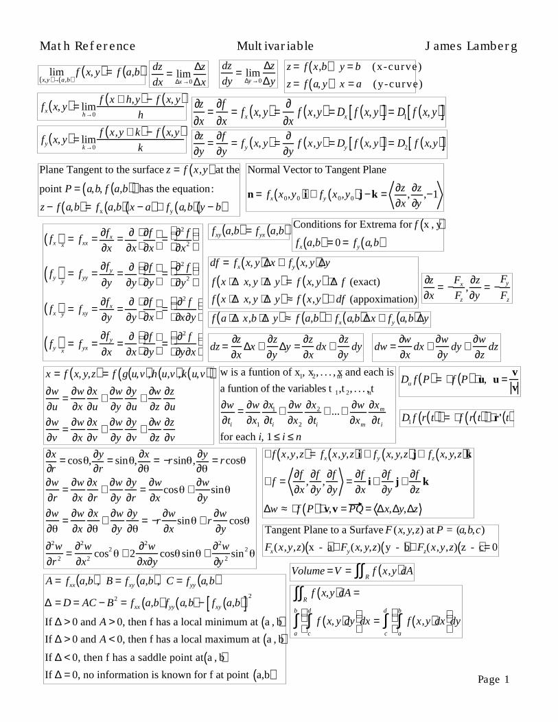
limx,y( )→ a,b( )
f x, y( ) = f a,b( ) dz
dx= lim
∆x →0
∆z
∆x
dz
dy= lim
∆y →0
∆z
∆y
fx x, y( ) = limh→0
f x + h,y( ) − f x, y( )h
fy x, y( ) = limk →0
f x,y + k( ) − f x,y( )k
∂z
∂x=
∂f
∂x= fx x, y( ) =
∂∂x
f x,y( ) = Dx f x, y( )[ ] = D1 f x, y( )[ ]∂z
∂y=
∂f
∂y= fy x, y( ) =
∂∂y
f x,y( ) = Dy f x, y( )[ ] = D2 f x,y( )[ ]
z = f x,b( ) y = b (x-curve)
z = f a, y( ) x = a (y-curve)
Plane Tangent to the surface z = f x,y( ) at the
point P = a,b, f a,b( )( ) has the equation:
z − f a,b( ) = fx a,b( ) x − a( ) + fy a,b( ) y − b( )
fx( )x
= fxx = ∂fx
∂x= ∂
∂x
∂f
∂x
= ∂2 f
∂x2
fy( )y
= fyy =∂fy
∂y= ∂
∂y
∂f
∂y
= ∂2 f
∂y2
fx( )y
= fxy =∂fx
∂y=
∂∂y
∂f
∂x
=
∂2 f
∂x∂y
fy( )x
= fyx =∂fy
∂x=
∂∂x
∂f
∂y
=
∂2 f
∂y∂x
fxy a,b( ) = fyx a,b( )
Normal Vector to Tangent Plane
n = fx x0,y0( )i + fy x0,y0( )j −k = ∂z
∂x,∂z
∂y,−1
Conditions for Extrema for f x , y( )fx a,b( ) = 0 = fy a,b( )
df = fx x, y( )∆x + fy x, y( )∆y
f x + ∆x, y + ∆y( ) = f x, y( ) + ∆f (exact)
f x + ∆x, y + ∆y( ) ≈ f x,y( ) + df (appoximation)
f a + ∆x,b + ∆y( ) ≈ f a,b( ) + fx a,b( )∆x + fy a,b( )∆y
dz =∂z
∂x∆x +
∂z
∂y∆y =
∂z
∂xdx +
∂z
∂ydy dw =
∂w
∂xdx +
∂w
∂ydy +
∂w
∂zdz
x = f x, y,z( ) = f g u,v( ),h u,v( ),k u,v( )( )∂w
∂u=
∂w
∂x
∂x
∂u+
∂w
∂y
∂y
∂u+
∂w
∂z
∂z
∂u
∂w
∂v=
∂w
∂x
∂x
∂v+
∂w
∂y
∂y
∂v+
∂w
∂z
∂z
∂v
w is a funtion of x1, x2, . . . , xm and each is
a funtion of the variables t 1,t 2, . . . , tn
∂w
∂ti
= ∂w
∂x1
∂x1
∂ti
+ ∂w
∂x2
∂x2
∂ti
+ ...+ ∂w
∂xm
∂xm
∂t i
for each i, 1 ≤ i ≤ n
∂x∂r
= cos ,∂y∂r
= sin ,∂x∂
= −rsin ,∂y∂
= rcos
∂w
∂r=
∂w
∂x
∂x
∂r+
∂w
∂y
∂y
∂r=
∂w
∂xcos +
∂w
∂ysin
∂w
∂=
∂w
∂x
∂x
∂+
∂w
∂y
∂y
∂= −r
∂w
∂xsin + r
∂w
∂ycos
∂2w
∂r 2=
∂2w
∂x2cos2 + 2
∂2w
∂x∂ycos sin +
∂2w
∂y 2sin2
∂z
∂x= −
Fx
Fz
,∂z
∂y= −
Fy
Fz
∇f x,y,z( ) = fx x,y,z( )i + fy x, y,z( )j+ fz x, y,z( )k
∇f =∂f
∂x,∂f
∂y,∂f
∂y=
∂f
∂xi +
∂f
∂yj +
∂f
∂zk
∆w ≈ ∇f P( )⋅ v,v = PQ = ∆x,∆y,∆z
Du f P( ) = ∇f P( ) ⋅ u, u =vv
D1 f r t( )( ) = ∇f r t( )( ) ⋅ r' t( )
Tangent Plane to a Surfave F (x, y,z) at P = (a,b,c)
Fx(x,y,z) x - a( ) + Fy(x, y,z) y - b( ) + Fz(x,y,z) z - c( ) = 0
A = fxx a,b( ), B = fxy a,b( ), C = fyy a,b( )∆ = D = AC − B2 = fxx a,b( ) fyy a,b( ) − fxy a,b( )[ ]2
If ∆ > 0 and A > 0, then f has a local minimum at a , b( )If ∆ > 0 and A < 0, then f has a local maximum at a , b( )If ∆ < 0, then f has a saddle point at a , b( )If ∆ = 0, no information is known for f at point a,b( )
Volume =V = f x,y( )R
∫∫ dA
f x,y( )R
∫∫ dA =
f x, y( )c
d
∫ dy
dx
a
b
∫ = f x,y( )a
b
∫ dx
dy
c
d
∫
Page 1
Math Reference Multivariable James Lamberg

LaGrange Multipliers
Constraint : g(x, y) = 0
Check Critical Points of F x ,y ,( ) = f x, y( ) − g x, y( )∂f∂x
,∂f∂y
= ∂g
∂x,∂g∂y
∂f
∂x−
∂g
∂x
= 0 ,
∂f
∂y−
∂g
∂y
= 0
x 2 + y 2 + z2 = a2 Sphere w/ Radius a
x 2
a2+
y 2
b2+
z2
c 2=1 Ellipsoid
x 2
a2+ y 2
b2− z 2
c2=1 Hyperboloid, 1 Sheet, z - a x i s
x 2
a2− y2
b2+ z 2
c2=1 Hyperboloid, 1 Sheet, y - a x i s
−x2
a2+
y2
b2+
z 2
c2=1 Hyperboloid, 1 Sheet, x - a x i s
x 2
a2− y2
b2− z2
c 2=1 Hyperboloid, 2 Sheets, yz-plane
− x2
a2+ y2
b2− z2
c 2=1 Hyperboloid, 2 Sheets, xz-plane
−x2
a2−
y 2
b2+
z2
c 2=1 Hyperboloid, 2 Sheets , xy-plane
A(y) = f x, y( )dxa
b
∫
A(x) = f x, y( )dyc
d
∫
Vertically Simple : f x , y( )dAR
∫∫
V = f x , y( )dydxy1 x( )
y 2 x( )
∫a
b
∫
Horizontally Simple : f x , y( )dAR
∫∫
V = f x , y( )dxdyx1 y( )
x 2 y( )
∫c
d
∫Volume Between Two Surfaces
V = z top − zbottom( )dAR
∫∫Polar : a ≤ r ≤ b, ≤ ≤
A =1
2a + b( ) a −b( ) −( ) = r∆r∆
V = f rcos ,rsin( )a
b
∫∫ rdrdmass = m = x,y( )
R∫∫ dA
Centroid : x, y( )x =
1
mx x, y( )dA
R∫∫
y = 1m
yR
∫∫ x, y( )dA
Polar Moments of Inertia
Ix = y 2 x, y( )dAR
∫∫Iy = x 2 x, y( )dA
R∫∫
Kinetic Energy due to Rotation
KErot =1
22r 2 dA =
R∫∫ 1
2I0
2
is angular speed
Radius of Gyration
ˆ r =I
mI is moment of inertia, m is mass around axis
ˆ x =I x
m ˆ y =
Iy
m
I0 = mˆ r 2 KE =1
2m ˆ r ( )2
mass = m = x, y,z( )T
∫∫∫ dV
Volume =V = dVT
∫∫∫Centroid : x, y, z( )x = 1
mx x, y,z( )dA
T∫∫∫
y =1
my x, y,z( )dA
T∫∫∫
z =1
mz x, y,z( )dA
T∫∫∫
Moments of Inertia
Ix = y 2 + z2( )T
∫∫∫ x, y,z( )dA
Iy = x 2 + z2( )T
∫∫∫ x, y,z( )dA
Iz = x2 + y2( )T∫∫∫ x, y,z( )dA
Cylindrical x = rcos , y = rsin , z = z
V = f rcos ,rsin ,z( )U
∫∫∫ rdzdrd
Sphererical x = sin cos ,y = sin sin ,z = cos
V = f sin cos , sin sin , cos( )U
∫∫∫ 2 sin d d d
Parametric
ru =∂r∂u
= xu,yu,zu =∂x
∂ui +
∂y
∂uj +
∂z
∂uk
rv = ∂r∂v
= xv, yv,zv = ∂x∂v
i + ∂y∂v
j+ ∂z∂v
k
Surface Area
A = a S( ) = 1+ ∂f∂x
2
+ ∂f∂y
2
dxdyR
∫∫
Cylindrical Surface Area
A = a S( ) = r2 + r∂f∂r
2
+ ∂f∂
2
drdR
∫∫Page 2
Math Reference Multivariable James Lamberg

Change of Variable
F x, y( )R
∫∫ dxdy
x = f u,v( ) y = g u , v( )u = h x, y( ) v = k x , y( )
Jacobian: JT u,v( ) =fu u,v( ) fv u,v( )gu u,v( ) gv u,v( )
=∂ x,y( )∂ u,v( )
F x, y( )dxdy =R
∫∫ F f u,v( ),g u,v( )( ) JT u,v( )dudvS
∫∫
F x, y( )dxdy =R
∫∫ G u,v( ) ∂ x, y( )∂ u,v( )
dudvS
∫∫
x = f u,v ,w( ) y = g u , v , w( ) z = hu,v ,w( )
Jacobian: JT u,v( ) =∂ x,y,z( )∂ u,v,w( )
=
∂x∂u
∂x∂v
∂x∂w
∂y
∂u
∂y
∂v
∂y
∂w∂z∂u
∂z∂v
∂z∂w
F x,y,z( )dxdyT
∫∫∫ dz = G u,v,w( ) ∂ x,y,z( )∂ u,v,w( )
dudvS
∫∫∫ dw
F x,y( ) = xi + yj = x 2 + y 2 = rVelocity Vector
v x,y( ) = −yi + xj( )Force Field
F x, y,z( ) = −krr 3
k = G ⋅ M
∇ af + bg( ) = a∇f + b∇g
∇ fg( ) = f∇g + g∇f
div F = ∇ ⋅F =∂P
∂x+
∂Q
∂y+
∂R
∂z
F x, y,z( ) = P x,y,z( )i + Q x,y,z( )j + R x, y,z( )k
∇ ⋅ aF + bG( ) = a∇ ⋅F + b∇ ⋅G,
∇ ⋅ fG( ) = f( ) ∇ ⋅G( ) + ∇f( )⋅ Gcurl F = ∇ ×F =
i j k∂∂x
∂∂y
∂∂z
P Q R
curl F = ∂R∂y
− ∂Q∂z
i + ∂P
∂z− ∂R
∂x
j + ∂Q
∂x− ∂P
∂y
k
∇ × aF + bG( ) = a ∇ ×F( ) + b ∇ ×G( ),∇ × fG( ) = f( ) ∇ ×G( ) + ∇f( ) ×G
f x, y,z( )ds = lim∆t →1
C
∫ f x ti*( ),y t i
*( ),z ti*( )( )∆si
f x, y,z( )ds = f x t( ),y t( ),z t( )( ) x ' t( )( )2+ y ' t( )( )2
+ z' t( )( )2
a
b
∫C
∫ dt
mass = x,y,z( )dsC
∫
x = 1m
x x,y,z( )dsC
∫
y =1
my x,y,z( )ds
C
∫
z = 1m
z x,y,z( )dsC
∫Centroid : x ,y ,z ( )
Moment of Inertia
I = w2 x,y,z( )dsC
∫w = w x,y,z( ) = ⊥ distance
from x , y , z( ) to axis
f x, y,z( )dx = f x t( ), y t( ),z t( )( )a
b
∫C
∫ ⋅ x ' t( )dt
f x, y,z( )dy = f x t( ), y t( ),z t( )( )a
b
∫C
∫ ⋅ y ' t( )dt
f x, y,z( )dz = f x t( ), y t( ),z t( )( )a
b
∫C
∫ ⋅ z' t( )dt
P x, y,z( )dx +C
∫ Q x, y,z( )dy + R x, y,z( )dz =
P x t( ), y t( ),z t( )( )a
b
∫ ⋅ x ' t( )dt +
Q x t( ), y t( ),z t( )( )a
b
∫ ⋅ y ' t( )dt +
R x t( ),y t( ),z t( )( )a
b
∫ ⋅ z' t( )dt
f x, y,z( )ds =−C
∫ f x, y,z( )dsC
∫Pdx + Qdy + Rdz =
−C
∫ − Pdx + Qdy + RdzC
∫Work
W = F ⋅ Tdsa
b
∫
W = Fdra
b
∫
W = Pdx + Qdy + Rdza
b
∫
∇f ⋅ drC
∫ = f r b( )( )C
∫ − f r a( )( ) = f B( ) − f A( )
F ⋅ TC
∫ ds = FC
∫ dr = Pdx + Qdy + Rdz
F ⋅ TC
∫ ds = F ⋅ TdsA
B
∫
W = F ⋅ TC
∫ ds = k w ⋅ TC
∫ ds
w = velocity vector
f x,y,z( ) = F ⋅ TdsC
∫ = F ⋅ Tdsx 0,y 0z( )0
x ,y,z( )
∫
W = F ⋅ drA
B
∫ =V A( ) −V B( )
Flux of a Vector
Field across C
F ⋅ n dsC
∫
n =dy
dsi −
dx
dsj
Page 3
Math Reference Multivariable James Lamberg

The Line Integral F ⋅ TC
∫ ds is independent
of path in the region D iff F = ∇f for some
funtion f defined on D
The vector field F defined on region D is conservative
provided that there exists a scalar funtion f defined on
D such that
F = ∇f
at each point of D, f is a potential funtion for FF ⋅ TA
B
∫ ds = ∇f ⋅ drA
B
∫ = f B( ) − f A( )
Continuous funtions P x,y( ) and Q x,y( ) have
continuous 1st order partials in R = x , y( ) |
a < x < b, c < y < d Then the vector field
F = Pi +Qj is conservative in R and has a
potential funtions f x, y( ) on R irr at each point
of R
∂P
∂y= ∂Q
∂x
Newton's First Law gives:
F r t( )( ) = mr" t( ) = mv' t( )dr = r ' t( ) dt = v t( )
F ⋅ drA
B
∫ =1
2m vB( )2 −
1
2m vA( )2
1
2m vA( )2 + V A( ) =
1
2m vB( )2 +V B( )
Green's Theorem
Pdx + Qdy = ∂Q
∂x− ∂P
∂y
R
∫∫C
∫ dA
Pdx = −∂P
∂ydA
R
∫∫C
∫
Qdy = + ∂Q∂x
dAR
∫∫C
∫
A =1
2−ydx + xdy = −
C
∫ ydx =C
∫ xdyC
∫
F ⋅ nds =∂M
∂x+
∂N
∂y
R
∫∫C
∫ dA
div F = ∇ ⋅F =∂M
∂x+
∂N
∂y
F ⋅ nds = ∇ ⋅FdAR
∫∫C
∫
∇ ⋅F x0, y0( ) = limr →0
1
πr2 F ⋅ ndsCr
∫
N =∂r∂u
×∂r∂v
=
i j k∂x
∂u
∂y
∂u
∂z
∂u∂x∂v
∂y∂v
∂z∂v
A ≈ N ui ,v i( )∆u∆vi=1
n
∑
m ≈ f r ui,vi( )( ) N ui ,v i( ) ∆u∆vi=1
n
∑
f x,y,z( )dS = f r ui,v i( )( ) N ui,vi( ) dudvD
∫∫S
∫∫
= f r ui,vi( )( ) ∂r∂u
×∂r∂v
dudvD
∫∫
dS = N ui,v i( ) dudv = ∂r∂u
× ∂r∂v
dudv
N =∂r∂u
×∂r∂v
=∂ y,z( )∂ u,v( )
i +∂ z, x( )∂ u,v( )
j+∂ x, y( )∂ u,v( )
k
f x,y,z( )dSS
∫∫
= f x u,v( ), y u,v( ),z u,v( )( ) ∂ y,z( )∂ u,v( )
2
+∂ z,x( )∂ u,v( )
2
+∂ x, y( )∂ u,v( )
2
S
∫∫ dudv
z = h x, y( ) in xy -plane
dS = 1+ ∂h∂x
2
+ ∂h∂y
2
dxdy
f x,y,z( )S
∫∫ dS = f x, y,h x,y( )( )S
∫∫ 1+∂h
∂x
2
+∂h
∂y
2
dxdy
R r ui,vi( )( )i=1
n
∑ cos N ui ,v i( )∆u∆v
≈ R r ui,vi( )( )D
∫∫ N ui ,v i( ) dudvn =
NN
= cos( )i + cos( )j + cos( )k
F ⋅ n = P cos + Qcos + R cos
Flux across S in
the direction of n
= F ⋅ ndSS
∫∫
Divergence Theorem
F ⋅ ndS =S
∫∫ ∇ ⋅FdVT
∫∫div F P( ) = lim
r→0
1
Vr
F ⋅ ndSSr
∫∫S o u r c e : div F P( ) > 0
S i n k : div F P( ) < 0
∂2u
∂x2+
∂2u
∂y2+
∂2u
∂z2=
1
k⋅∂u
∂t
k =Thermal Diffusivity
F ⋅ TdS = curlF( )R
∫∫C
∫ ⋅ kdA
Page 4
Math Reference Multivariable James Lamberg

cos = n ⋅ i =N ⋅ iN
=1
N∂ y,z( )∂ u,v( )
cos = n ⋅ j =N ⋅ iN
=1
N∂ z,x( )∂ u,v( )
cos = n ⋅ k =N ⋅ iN
=1
N∂ x, y( )∂ u,v( )
P x,y,z( )S
∫∫ dydz = P x,y,z( )S
∫∫ cos dS = P r u,v( )( )D
∫∫ ∂ y,z( )∂ u,v( )
dudv
Q x,y,z( )S
∫∫ dydx = Q x,y,z( )S
∫∫ cos dS = Q r u,v( )( )D
∫∫ ∂ z,x( )∂ u,v( )
dudv
R x, y,z( )S
∫∫ dxdy = R x,y,z( )S
∫∫ cos dS = R r u,v( )( )D
∫∫ ∂ x, y( )∂ u,v( )
dudv
Pdydz + Qdzdx + RdxdyS
∫∫= P cos + Qcos + Rcos( )dS
S
∫∫
= P∂ y,z( )∂ u,v( )
+ Q∂ z,x( )∂ u,v( )
+ R∂ x,y( )∂ u,v( )
dudv
D
∫∫
F ⋅ ndS = Pdydz + Qdzdx + RdxdyS
∫∫S
∫∫
= −P∂z∂x
− Q∂z∂y
+ R∂z∂z
D
∫∫ dxdy
Heat -Flow Vector
q = −K∇u
K =Heat Conductivity
q ⋅ ndS = − K∇uS
∫∫S
∫∫ ⋅ ndS
Gauss' Law for flux
= F ⋅ ndS = −4πGMS
∫∫Gauss' Law for electric fields
= E ⋅ ndS =Q
0S
∫∫
P cos + Qcos + Rcos( )S
∫∫ dS
= Pdydz + Qdzdx + Rdxdy( )S
∫∫
= ∂P
∂x+ ∂Q
∂y+ ∂R
∂z
dV
T
∫∫∫
PdydzS
∫∫ = ∂P∂xT
∫∫∫ dV
QdzdxS
∫∫ =∂Q
∂yT
∫∫∫ dV
RdxdyS
∫∫ = ∂R∂zT
∫∫∫ dVS3 is SA between S1 and S2
Rdxdy =s3
∫∫ Rcos dS =s3
∫ 0∫Rdxdy =
s2
∫∫ R x, y,z2 x, y( )( )dxdys2
∫∫Rdxdy =
s1
∫∫ − R x,y,z1 x, y( )( )dxdyD
∫∫
∇ ⋅FT
∫ dV = F ⋅ ndSS
∫∫∫∫= F ⋅ n2dS
S2
∫∫ − F ⋅ n1dSS1
∫∫
F ⋅ ndS =S
∫∫ F ⋅ ndSSa
∫∫
= − GMr
r3
⋅ rr
dSSa
∫∫
= −GMra2
1dSSa
∫∫= −4πGM
Stokes' Theorem
F ⋅ TdS = curlF( )S
∫∫C
∫ ⋅ ndA
Pdx + Qdy + Rdz =∂R
∂y−
∂Q
∂z
S
∫∫C
∫ dydz +∂P
∂z−
∂R
∂x
dzdx +
∂Q
∂x−
∂P
∂y
dxdy
Pdx = −∂P
∂y
∂y
∂y+
∂P
∂z
∂z
∂y
D
∫∫C
∫ dxdy
∂P
∂zdzdy − ∂P
∂zdxdy
S
∫∫
= − ∂P∂z
∂z∂y
− ∂P∂y
∂y∂y
D
∫∫ dxdycurlF( ) ⋅ n P( ) = limr→0
1
πr 2 F ⋅ TdsC r
∫
Γ C( ) = F ⋅ TdsC
∫
curlF( ) ⋅ n P*( ) ≈Γ Cr( )πr2
A vector field is irrotational iff
It is conservative and
F = ∇ for some scalar
x, y,z( ) = F ⋅ TC1
∫ ds div v dVT
∫∫∫ = v ⋅ ndS = 0S
∫∫
div ∇( ) =∂2
dx 2 +∂2
dy2 +∂2
dz 2 = 0
∂2u
dx2+ ∂2u
dy 2+ ∂2u
dz2= 0
Page 5
Math Reference Multivariable James Lamberg

Page 1
Physics Reference Electricity & Magnetism James Lamberg
F =q1 ⋅ q2
4π ⋅ 0 ⋅ r 2
Electric Charge
Charges with the same electrical
sign repel each other, and charges
with opposite electrical sign attractk =
1
4π ⋅ 0
≈ 9 ×10⁹ N ⋅ m 2
C
e− ≈1.6 ×10⁻¹⁹C A shell of uniform charge
attracts or repels a charged
particle that is outside the
shell as if all the shell's charge
were concentrated at its center
A shell of uniform charge
exerts no electrostatic force
on a charged particle that is
located inside the shell.
q = n ⋅ e, n= ±1,±2 , . . .
Electric Fields
E = Fq0
Electric field lines extend
away from positive charge
and toward negative charge
Point Charge
E = kq
r2
Electric Dipole
p = Dipole Moment
E = k2pz 3
≈3 p ⋅ ˆ r ( ) − p
4π ⋅ 0 ⋅ z3
Charged Ring
E = q ⋅ z
4π ⋅ 0 z2 + R2( )3 2
Charged Disk
E =2 0
1− z
z2 + R2
Torque
t = p ×E
Potential Energy
Of A Dipole
U = −p ⋅ E
Gauss' Law : 0 ⋅ Φ =Qenclosed
Flux = Φ = E ⋅ dA∫ =Qenclosed
0
Conducting Surface
E =0
Line Of Charge
E =2π ⋅ 0 ⋅ r
Sheet Of Charge
E =2 0
Spherical Shell
Field At r ≥ R
E = q4π ⋅ 0 ⋅ r 2
Spherical Shell
Field At r < R
E = 0
Electric Potential
∆U = q ⋅ ∆W
∆V =V f −Vi = −W
q
Vi = −W∞
q
Electric Potential
V f −Vi = − E ⋅ dsi
f
∫ = VElectric Potential
V = kq
r= k ⋅ qi
rii=1
n
∑
Electric Diplole
V = kp ⋅ cos( )
r2
V = k ⋅dq
r∫ ES = −
V
sE = − ∇V
U = W = kq1 ⋅ q2
rCapacitance
C =Q
V
Parallel Plate
Capacitor
C = 0 ⋅ Ad
Cylindrical
Capacitor
C = 2π ⋅ 0
Lln b a( )
Spherical
Capacitor
C = 4π ⋅ 0
a ⋅ bb − a
Isolated Sphere
C = 4π ⋅ 0 ⋅ R
Parallel
Ceff = Ci
i=1
n
∑Series
1
Ceff
=1
Cii=1
n
∑Potential Energy
U =Q2
2C=
1
2C ⋅V 2
Energy Density
u =Q2
2C=
1
2 0 ⋅ E 2 Dielectric
C = ⋅ Cair
0 ⋅ k ⋅ E ⋅ dA = Qenclosed∫
Current
i =dq
dt
Current Density
i = J ⋅ dA∫Current Density
J =i
A, Constant
J = n ⋅ e ⋅ vdriftResistance
R =V
i, Ohm's Law Resistivity
=E
J
Conductivity
=1
E = ⋅ J
Resistance is a property of an object
Resistivity is a property of a materialR =
L
A− 0 = 0 ⋅ T −T0( )Power, Rate Of Transfer
Of Electrical Energy
P = i ⋅ V
Resistive Dissapation
P = i2 ⋅ R =V 2
R
Resistivity Of A Conductor
(Such As Metal)
= me2 ⋅ n ⋅
EMF
=dW
dq
i =R
Kirchoff's Loop Rule
The sum of the changes in
potential in a loops of a
circuit must be zero
Parallel
1
Reff
=1
Rii=1
n
∑
Series
Reff = Ri
i=1
n
∑EMF Power
Pemf = i ⋅Kirchoff's Junction Rule
The sum of the currents entering
any junction must equal the sum
of the currents leaving that junctionCharging A Capacitor
q t( ) = C ⋅ 1−e−t R ⋅C( )i t( ) =
R⋅ e− t R ⋅C
i t( ) =dq
dt
Charging A Capacitor
VC = 1− e− t R ⋅C( )
Discharging A Capacitor
q t( ) = q0 ⋅ e−t R ⋅C
i t( ) = −q0
R ⋅ C⋅ e− t R ⋅C
Page 2
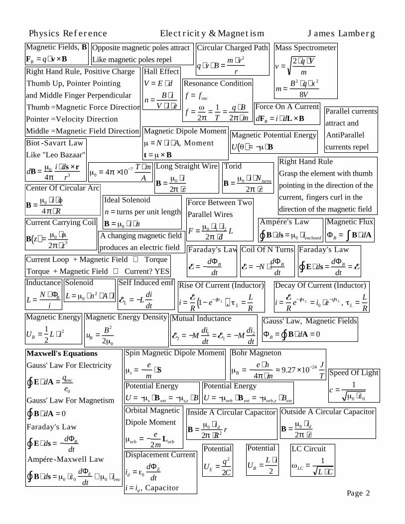
Physics Reference Electricity & Magnetism James LambergMagnetic Fields, B
FB = q ⋅ v ×B
Right Hand Rule, Positive Charge
Thumb Up, Pointer Pointing
and Middle Finger Perpendicular
Thumb =Magnetic Force Direction
Pointer =Velocity Direction
Middle =Magnetic Field Direction
Opposite magnetic poles attract
Like magnetic poles repel
Hall Effect
V = E ⋅ d
n = B ⋅ iV ⋅ l ⋅ e
Circular Charged Path
q ⋅ v ⋅ B =m ⋅ v2
r
Mass Spectrometer
v =2 ⋅ q ⋅V
m
m =B2 ⋅ q ⋅ x 2
8V
Resonance Condition
f = fosc
f =2π
= 1T
= q ⋅ B2π ⋅ m
Force On A Current
dFB = i ⋅ dL ×B
Magnetic Dipole Moment
= N ⋅ i ⋅ A, Moment
t = × B
Magnetic Potential Energy
U( ) = − ⋅ BBiot -Savart Law
Like "Leo Bazaar"
dB = 0
4πi ⋅ ds ×r
r3 0 = 4π ×10−7 T ⋅ m
A
Long Straight Wire
B = 0 ⋅ i
2π ⋅r
Right Hand Rule
Grasp the element with thumb
pointing in the direction of the
current, fingers curl in the
direction of the magnetic field
Parallel currents
attract and
AntiParallel
currents repel
Center Of Circular Arc
B = 0 ⋅ i ⋅4π ⋅ R
Force Between Two
Parallel Wires
F = 0 ⋅ i1 ⋅ i2
2π ⋅dL
Ampére's Law
B ⋅ ds∫ = 0 ⋅ ienclosed
Ideal Solenoid
n = turns per unit length
B = 0 ⋅ i ⋅ n
Torid
B = 0 ⋅ i ⋅ N turns
2π ⋅r
Current Carrying Coil
B z( ) = 0 ⋅2π ⋅ z3
Current Loop + Magnetic Field ⇒ Torque
Torque + Magnetic Field ⇒ Current? YES
Magnetic Flux
ΦB = B ⋅ dA∫Faraday's Law
= −dΦB
dt
Coil Of N Turns
= −N ⋅dΦB
dt
A changing magnetic field
produces an electric field Faraday's Law
E ⋅ ds∫ =dΦB
dt=
Inductance
L =N ⋅ ΦB
i
Solenoid
L = 0 ⋅ n2 ⋅ A ⋅ l
Self Induced emf
L = −Ldi
dt
Rise Of Current (Inductor)
i =R
1− e− t L( ), L =L
R
Decay Of Current (Inductor)
i =R
e− t L = i0 ⋅ e−t L , L =L
RMagnetic Energy
UB =1
2L ⋅ i2
Magnetic Energy Density
uB = B2
2 0
Mutual Inductance
2 = −Mdi1dt
= 1 = −Mdi2
dt
Gauss' Law, Magnetic Fields
ΦB = B ⋅ dA∫ = 0
Maxwell's Equations
Gauss' Law For Electricity
E ⋅ dA∫ = qenc
e0
Gauss' Law For Magnetism
B ⋅ dA∫ = 0
Faraday's Law
E ⋅ ds∫ = −dΦB
dtAmpére-Maxwell Law
B ⋅ ds∫ = 0 ⋅ 0
dΦE
dt+ 0 ⋅ ienc
Spin Magnetic Dipole Moment
s = −e
m⋅ S
Bohr Magneton
B = −e ⋅ h
4π ⋅ m≈ 9.27 ×10⁻²⁴ J
TPotential Energy
U = − s ⋅ B ext = − s,z ⋅ B
Orbital Magnetic
Dipole Moment
orb = − e2m
Lorb
Potential Energy
U = − orb ⋅ B ext = − orb,z ⋅ Bext
Inside A Circular Capacitor
B = 0 ⋅ id
2π ⋅R2r
Outside A Circular Capacitor
B = 0 ⋅ id
2π ⋅r
Displacement Current
id = 0
dΦE
dti = id , Capacitor
Speed Of Light
c =1
0 ⋅ 0
Potential
UE =q2
2C
Potential
UB =L ⋅ i
2
LC Circuit
LC = 1
L ⋅ C

Page 3
Physics Reference Electricity & Magnetism James LambergRLC Circuit
Ldi
dt+ i ⋅ R +
Q
C= 0
q t( ) = A ⋅ e−t 2 LR ⋅ cos LC ⋅ t −( )LR =
L
R
= LC
2 −1
2 LR
2LC Circuit
Ld2qdt2
+ qC
= 0
q t( ) = Q ⋅ cos ⋅ t +( )i t( ) = − ⋅ Q ⋅ sin ⋅ t +( )
UE = Q2
2C⋅ cos2 ⋅ t +( )
UB =Q2
2C⋅ sin2 ⋅ t +( )
U =Q2
2Ce−t LR
RLC Circuit w/ AC
Ldidt
+ i ⋅ R + QC
= B ⋅ sin d ⋅ t( )i t( ) = iB ⋅ sin d ⋅ t −( )iB = B Z
Capacitive Reactance
XC = 1
d ⋅ CInductive Reactance
XL = d ⋅ L
Phase Constant
tan( ) =XL − XC
R
Impedance
Z = XL − XC( )2 + R2
Current Amplitude
i = B
Z
Resonance
d = = 1
L ⋅ C
rms current
irms = i
2Average Power
Pav = irms
2 ⋅ R
Not "rms Power"rms potential
Vrms = V
2, rms = B
2
Average Power
Pav = rms ⋅ irms ⋅ cos( )
Transformer Voltage
V2nd =V1st
N2nd
N1st
Transformer Current
i2nd = i1st
N1st
N2nd
Resistance Load at Generator
Req = N1st
N2nd
2
⋅ R
Maxwell's Equations (Derviative)
∇ •E =0
∇ •B = 0
∇ ×E = − Bt
∇ ×B = 0 ⋅ J +1
c2⋅
Edt
Maxwell's Equations (Integral)
E ⋅ dA∫ = qenc
0
B ⋅ dA∫ = 0
E ⋅ ds∫ = −ddt
B ⋅ dA∫
B ⋅ ds∫ = 0 ⋅ ienc +1
c2
d
dtE ⋅ dA∫
Average Power relates
to the heating effect
RMS Power, while it
can be calculated is worthless

Page 1
Math Reference Sequences & Series James LambergP and Q is P ∧Q
P or Q is P ∨Q
not P is ¬P
if P then Q is P ⇒ Q
P if and only if Q is P ⇔Q
¬ P ∧ Q( ) is ¬P ∨¬Q
¬ P ∨ Q( ) is ¬P ∧¬Q
¬ P ⇒ Q( ) is P ∧ ¬Q
¬Q ⇒ ¬P is contrapositive of P ⇒ Q
and these are equivalent
Q ⇒ P is converse of P ⇒ Q
and these may not be equivalent
P is a necessary condition for Q : Q ⇒ P
P is a sufficient condition for Q : P ⇒ Q
N = Set of positive int egers
Z = Set of all i n tegers
Q = Set of rational numbers
R = Set of real numbers
Existential Quantifier :
∀x : for all/every x
Universal Quantifier :
∃x : there exists x
∈: element of
Mathematical Induction :
1) ∀n ∈ N, P rove Base Case that
P 1( ) is true
2)Assume P n( ) and ∀n ∈ N,
show P n( ) ⇒ P n +1( )
The set A is finite if A = ∅ or for some n ∈ N,
A has exactly n members.
The set A is infinite if A is not finite.
Pr inciple of Mathematical Induction
Let P n( ) be a mathematical statement, if
a) P 1( ) is true, and
b) for every n ∈ N
P n( ) ⇒ P n +1( ) is true,
then P n( ) is true for every n ∈ N
Strong Induction
1) P 1( ) is true, and
2) for each n ∈ N, if each P 1( ),...,P n( ) is true[ ], then P n +1( ) is true, then P n( ) is true ∀n ∈ N
Well Ordering Property of N :
Every nonempty subset of N has
a smallest memeber
Bounds: Suppose A is a set of real numbers
1) r ∈ R is an upper bound of A if no member
of A is bigger than r : ∀x ∈ A x ≤ r[ ]2) r ∈ R is a lower bound of A if no member
of A is smaller than r : ∀x ∈ A r ≤ x[ ]3) A is bounded above if ∃r ∈ R which is an
upper bound of A
A is bounded below if ∃r ∈ R which is a
lower bound of A
A is bounded if if is bounded above and below
The least upper bound, r, of A is the supremum
of and is denoted sup A, that is r =sup A if:
a) r is an upper bound of A, and
b) r ≤ r' for every upper bound r' of A
The greatest lower bound, r, of A is the infimum
of and is denoted inf A, that is r =inf A if:
a) r is a lower bound of A, and
b) r ≥ r' for every upper bound r' of A
sup A exists if A has a least upper bound and
inf A exists if A has a greatest lower bound
Completeness Axiom:Every nonempty
subset of R which is bounded above has
a least upper bound
Archimedean Property of N :
N is not bounded above
For every positive real number x, there is
some positive i n teger n such that 0 <1
n< x
For all real numbers x and y such that x < y,
there is a rational number r such that x < r < y
For all real numbers x and y such that x < y,
there is an irrational number ir such that x < ir < y
There is no rational number r such that r 2 = 2
There is a real number x such that x2 = 2Let n ∈ N. For every real number y > 0,
there is a real number x > 0 such that xn = y
Completeness Axiom Corollary :Every
nonempty subset of R which is bounded
below has a greatest lower bound

Page 2
Math Reference Sequences & Series James LambergA sequence is a function whose domain is a
set of the form n ∈ Z : n ≥ k , where k ∈ Z
If s is a sequence, sn is the value of the
sequence at arg ument n .
Given an and bn with domain D :
an + bn is sn = an + bn ∀n ∈ D
an − bn is sn = an − bn ∀n ∈ D
an ⋅ bn is sn = an ⋅ bn ∀n ∈ D
an
bn
is sn =
an
bn
∀n ∈ D,bn ≠ 0
c ⋅ an is sn = c ⋅ an ∀n ∈ D
Definition of a Limit :
Let L be a real number.
limn→∞
sn = L iff
∀ > 0 ∃n0 ∀n ≥ n0 sn − L <[ ]The sequence s converges to L if lim
n →∞sn = L .
The sequence s is convergent if there is some
L such that s converges to L.
The sequence s is divergent if is is not convergent
limn→∞
sn = L is
limsn = L is
sn → L
If lim sn = L0 and sn = L1, then L0 = L1
The sequence sn is bounded if
there is some r ∈ R such that sn ≤ r
for all n in the domain of sn .If a sequence is convergent,
then it is bounded
Suppose l i msn = L1, and lim tn = L2, and c ∈ R.
a) l imsn + tn( ) = L1 + L2
b) lim c ⋅ sn( ) = c ⋅ L1
c) lim sn ⋅ tn( ) = L1 ⋅ L2
d) limsn
tn
=
L1
L2
, L2 ≠ 0 and ∀n tn ≠ 0[ ]
Suppose that for all sufficiently large n,
an ≤ bn ≤ cn
If lim an = L and limcn = L then limbn = L
If lim sn = 0 , then l i msn = 0
Suppose : l i man = L, and f is a function which
is continuous at L, and for each n, an is in the
domain of f . Then lim f an( ) = f L( )f is continuous at x if for any > 0 there exists
some > 0 so that if z - x < , then f z( ) - f x( ) <The set of reals R is the completion of the set
of i n tegers Q. Or R = sup A | A ⊆ Q
Let sn = f n( ). If limx →∞
f x( ) = L, then lim sn = L
Let sn = f1
n
. If lim
x →0+f x( ) = L, then l i msn = L
Let sn be a sequence. lim sn = ∞ if :
∀M∃n0∀n ≥ n0 sn ≥ M[ ]limsn = − ∞ if :
∀M∃n0∀n ≥ n0 sn ≤ M[ ]The sequence sn is:
increasing if for all n, sn ≤ sn+1
strictly increasin g if for all n, sn < sn+1
decreasin g if for all n, sn ≥ sn +1
strictly decreasin g if for all n, sn > sn+1
monotonic if any of the above are true
Suppose sn is monotonic. Then
sn converges iff it is bounded.
Re cursively Defined Sequence is
defined in terms of sn for each n .
The sequence sn is a Cauchy sequence
if for every > 0, there is some n0 such
that sm - sn < for all m, n ≤ n0
Cauchy sequences are bounded and converge
f x( )a
∞
∫ dx = limsn = limn →∞
f x( )a
n
∫ dx
f is continuous and x ≥ a
If f x( )a
∞
∫ dx converges
then f x( )a
∞
∫ dx converges
If lim a i ≠ 0, then a ii=1
∞
∑ is divergent
Geometric Series : a and r are real
a ⋅ r i, with r being the ratioi =0
∞
∑
Page 3
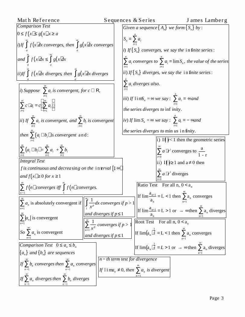
Math Reference Sequences & Series James LambergComparison Test
0 ≤ f x( ) ≤ g x( ), x ≥ a
i)If f x( )a
∞
∫ dx converges, then g x( )a
∞
∫ dx converges
and f x( )a
∞
∫ dx ≤ g x( )a
∞
∫ dx
ii)If f x( )a
∞
∫ dx diverges, then g x( )a
∞
∫ dx diverges
Given a sequence An we form Sn by :
Sn = aii=1
n
∑i) If Sn converges, we say the i n finite series :
aii=1
n
∑ converges to aii=1
n
∑ = limSn , the value of the series
ii) If Sn diverges, we say the i n finite series :
aii=1
n
∑ diverges also.
iii) If l i mSn = ∞ we say : aii=1
n
∑ = ∞ and
the series diverges to inf inity.
iv) If lim Sn = ∞ we say : aii=1
n
∑ = − ∞ and
the series diverges to min us i n finity.
i) Suppose aii=1
∞
∑ is convergent, for c ∈ R,
c ⋅ aii=1
∞
∑ = c aii=1
∞
∑
ii) If aii=1
∞
∑ is convergent, and bii=1
∞
∑ is convergent
then ai + bi( )i=1
∞
∑ is convergent and :
ai + bi( )i=1
∞
∑ = aii=1
∞
∑ + bii=1
∞
∑
i ) If r< 1 then the geometric series
a ⋅ r i
i= 0
∞
∑ converges to a
1 - r
ii) If r≥1 and a ≠ 0 then
a ⋅ r i
i= 0
∞
∑ diverges
1
x p1
∞
∫ dx converges if p > 1
and diverges if p ≤1
n − th term test for divergence
If l i m an ≠ 0, then an
n =1
∞
∑ is divergent
Integral Test
f is continuous and decreasing on the i n terval 1, ∞[ )and f x( ) ≥ 0 for x ≥1
f n( ) converges iff f n( )1
∞
∫n =1
∞
∑ converges.
1
x pn=1
∞
∑ converges if p > 1
and diverges if p ≤1
Comparison Test 0 ≤ an ≤ bn
an and bn are sequences
If bnn =1
∞
∑ converges then ann =1
∞
∑ converges
If ann =1
∞
∑ diverges then bnn =1
∞
∑ diverges
Ratio Test For all n, 0 < an
If liman+1
an
= L <1 then an convergesn=1
∞
∑
If liman+1
an
= L >1 or → ∞ then an divergesn=1
∞
∑Root Test For all n, 0 < an
If lim an( )1
n = L <1 then an convergesn=1
∞
∑
If lim an( )1
n = L >1 or → ∞ then an divergesn=1
∞
∑
an is absolutely convergent ifn=1
∞
∑
an is convergentn=1
∞
∑
So an is convergentn=1
∞
∑
Limit - Comparison Test
For all n, 0< an and 0 < bn
If liman
bn
= L > 0, L ∈ ℜ
an
n =1
∞
∑ converges then bn
n =1
∞
∑ converges
If liman
bn
= 0
bnn =1
∞
∑ converges then ann =1
∞
∑ converges
If liman
bn
→ ∞
bnn =1
∞
∑ diverges then ann =1
∞
∑ diverges
Math Reference Sequences & Series James Lamberg
Page 4
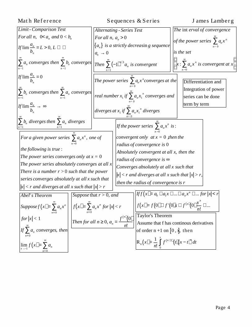
Alternating - Series Test
For all n, an > 0
an is a strictly decreasin g sequence
an → 0
Then −1( )n+1an is convergent
n =1
∞
∑
The power series an x n
n= 0
∞
∑ converges at the
real number x1 if an x1
n
n= 0
∞
∑ converges and
diverges at x1 if an x1n
n= 0
∞
∑ diverges
For a given power series an xn
n =0
∞
∑ , one of
the following is true :
The power series converges only at x = 0
The power series absolutely converges at all x
There is a number r > 0 such that the power
series converges absolutely at all x such that
x < r and diverges at all x such that x > r
If the power series an xn
n =0
∞
∑ is :
convergent only at x = 0 , then the
radius of convergence is 0
Absolutely convergent at all x, then the
radius of convergence is ∞Converges absolutely at all x such that
x < r and diverges at all x such that x > r,
then the radius of convergence is r
The int erval of convergence
of the power series an x n
n= 0
∞
∑
is the set
x : an x n
n =0
∞
∑ is convergent at x
Differentiation and
Integration of power
series can be done
term by term
Abel' s Theorem
Suppose f x( ) = an xn
n= 0
∞
∑for x < 1
If ann= 0
∞
∑ converges, then
limx →-1
f x( ) = an
n= 0
∞
∑
Suppose that r > 0, and
f x( ) = ann= 0
∞
∑ xn for x < r
Then for all n ≥ 0, an =f n( ) 0( )
n!
If f x( ) = a0 + a1x + ...+ an xn + ... for x < r
f x( ) = f 0( ) + f ' 0( )x + f n( ) 0( ) x n
n!+ ...
Taylor's Theorem
Assume that f has continous derivatives
of order n +1 on 0 , x[ ], then
Rn x( ) = 1n!
f n +1( ) t( ) x − t( )ndt
0
x
∫
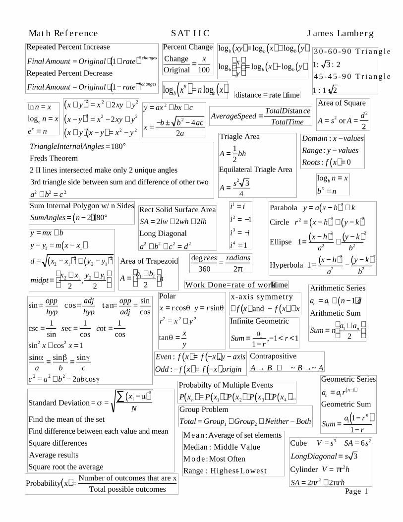
Percent Change
Change
Original=
x
100
Repeated Percent Increase
Final Amount = Original ⋅ 1+ rate( )# changes
Repeated Percent Decrease
Final Amount = Original ⋅ 1− rate( )#changes
logb n = x
b x = n
logb xy( ) = logb x( ) + logb y( )
logb
x
y
= logb x( ) − logb y( )
logb xn( ) = n logb x( )ln n = x
loge n = x
ex = n
distance = rate ⋅ time
AverageSpeed =TotalDistance
TotalTime
x + y( )2 = x 2 + 2xy + y2
x − y( )2 = x2 −2xy + y2
x + y( ) x − y( ) = x2 − y 2
y = ax 2 + bx + c
x = −b ± b2 − 4ac2a
TriangleInternalAngles =180°Freds Theorem
2 II lines intersected make only 2 unique angles
3rd triangle side between sum and difference of other two
a2 + b2 = c 2
3 0 - 6 0 - 9 0 T r i a n g l e
1: 3 : 2
4 5 - 4 5 - 9 0 T r i a n g l e
1 : 1 : 2
Triagle Area
A =1
2bh
Equilateral Triagle Area
A = s2 34
Area of Square
A = s2 or A =d2
2
Area of Trapezoid
A = b1 + b2
2
h
Sum Internal Polygon w/ n Sides
SumAngles = n − 2( )180°Rect Solid Surface Area
SA = 2lw + 2wh + 2lh
Long Diagonal
a2 + b2 + c2 = d2
Cube V = s3 SA = 6s2
LongDiagonal = s 3
Cylinder V = πr2h
SA = 2πr 2 + 2πrh
y = mx + b
y − y1 = m x − x1( )d = x2 − x1( )2 + y2 − y1( )2
midpt =x2 + x1
2,y2 + y1
2
Parabola y = a x − h( )2 + k
Circle r 2 = x − h( )2 + y − k( )2
Ellipse 1=x − h( )2
a2+
y − k( )b2
2
Hyperbola 1=x − h( )2
a2−
y − k( )b2
2
sin = opp
hyp cos= adj
hyp t an= opp
adj= sin
cos
csc =1
sin sec =
1
cos cot =
1
cos
sin2 x + cos2 x =1
sina
= sinb
= sinc
c 2 = a2 + b2 − 2abcos
Work Done=rate of work⋅ time
deg rees
360=
radians
2π
Polar
x = rcos y = rsin
r2 = x 2 + y 2
tan = x
y
Even : f x( ) = f −x( ), y − axis
Odd : − f x( ) = f −x( ),origin
x-axis symmetry
∃ f x( ) and − f x( ) ∀x
Domain : x −values
Range : y − values
Roots : f x( ) = 0
Standard Deviation = =x i −( )2∑N
Find the mean of the set
Find difference between each value and mean
Square differences
Average results
Square root the average
Probability x( ) =Number of outcomes that are x
Total possible outcomes
Probabilty of Multiple Events
P xn( ) = P x1( )⋅ P x2( ) ⋅ P x3( ) ⋅ P x4( )...Group Problem
Total = Group1 + Group2 + Neither − Both
Mean : Average of set elements
Median : Middle Value
M o d e : Most Often
Range : Highest-Lowest
Arithmetic Series
an = a1 + n −1( )dArithmetic Sum
Sum = na1 + an
2
Geometric Series
an = a1rn−1( )
Geometric Sum
Sum =a1 1− r n( )
1− r
Contrapositive
A → B ∴ ~ B →~ A
Infinite Geometric
Sum =a1
1− r,−1< r <1
i1 = i
i2 = −1
i3 = −ii4 =1
Page 1
Math Reference SAT IIC James Lamberg


![=T[f (x, y)]jjackson.eng.ua.edu/courses/ece482/lectures/LECT05-2.pdfimage, T is an operator on f defined over a neighborhood of point (x,y) g(x,y) =T[f (x,y)] Electrical & Computer](https://static.fdocuments.net/doc/165x107/5fa635054c3d6001795812fc/tf-x-y-image-t-is-an-operator-on-f-defined-over-a-neighborhood-of-point-xy.jpg)


![o µ ] } v W z x I s F t F x · 2020. 3. 16. · ^ } o µ ] } v W A B y F t F u s r w z r s C U A B z F s v F t C U A N F x u r v { F t z w O U A H w F u t r z x s F t F x I î Æ](https://static.fdocuments.net/doc/165x107/60c17ac05650b939bc059587/o-v-w-z-x-i-s-f-t-f-x-2020-3-16-o-v-w-a-b-y-f-t-f-u-s-r-w.jpg)