New tax policy needed to help

Wisconsin prosper

By Suffolk University’s Beacon Hill Institute for Public Policy Research

. W i s c o n s i n P o l i c y R e s e a R c h i n s t i t u t e .

Can State

Pull ItsPunches?

Volume 27 Number 2 . September 2014

WPRI R E P O R T

October 2009 | Volume 22 | Number 7

Wisconsin Policy Research Institute

WPRI Mission Statement

The Wisconsin Policy Research Institute Inc., established in 1987, is a nonpartisan, not-for-profit institute working to engage and energize Wisconsinites and others in discussions and timely action on key public policy issues critical to the state’s future, its growth and prosperity. The institute’s research and public education activities are directed to identify and promote public policies in Wisconsin that are fair, accountable and cost-effective.

Through original research and analysis and through public opinion polling, the institute’s work will focus on such issue arenas as state and local government tax policy and spending and related program account-ability, consequences and effectiveness. It will also focus on health care policy and service delivery; education; transportation and economic development; welfare and social services; and other issues currently or likely to significantly impact the quality of life and future of the state.

The institute is guided by a belief that competitive free markets, limited government, private initiative, and personal responsibility are essential to our democratic way of life.

Contact Information Address 633 W. Wisconsin Ave. Suite 330 Milwaukee, WI 53203 Phone 414-225-9940 Email wpri@wpri.org Website

www.wpri.org

Board of Directors

Thomas Howatt, Chairman David Baumgarten

Ave Bie Catherine C. Dellin

Jon Hammes Michael T. Jones

James Klauser David J. Lubar Maureen Oster Timothy Sheehy Gerald Whitburn

Edward Zore Mike Nichols, President

President’s Notes Creatures of habit and tradition, Wisconsinites are bound to a tax system that reflects our past and ignores our future.

Wisconsin has become more competitive on the tax front than it once was. The passage of Act 145 in March brought the total amount of tax reductions in the last few years to nearly $2 billion — not an inconsequential sum. And yet, the state still imposes a larger tax burden on its citizens and businesses than most other places.

Economists from Suffolk University’s Beacon Hill Institute for Public Policy have determined through economic modeling that we would benefit long-term from further tax cuts. And yet, they’ve found, Wisconsin doesn’t just suffer from high taxes. It suffers from the wrong tax mix.

While our sales taxes are lower than those in two-thirds of other states, our income and prop-erty tax burdens remain significantly higher — an economically detrimental combination. There is a clear need for Wisconsin to step back on firm ground and consider a new tax mix that lowers more harmful income and property taxes and broadens the sales tax base.

Tax changes are always controversial, and there will undoubtedly be consternation in some corners. Short-term concerns, however, should not obscure the need for a long-term view. In the past, changes to the tax code have too often been made simply to take advantage of temporary budget surpluses or to somehow patch over unforeseen deficits. The state has failed to ask a funda-mental and all-important question: Politics and special interests aside, what is the best tax structure for long-term prosperity in the state of Wisconsin?

This paper provides the data and analysis to help frame that discussion at a pivotal time.

by Paul Bachman, MSIE, Michael Head, MSEP,

Frank Conte, MS, and David G. Tuerck, Ph.D.

Can State Pull Its Punches? New Tax Policy Needed to Help Wisconsin Prosper

Mike Nichols President

Table of Contents

Executive Summary .......................................................................................................2

How Wisconsin Compares With Other States ...............................................................3

The Economics of State Taxes ........................................................................................5

The Fiscal Policy Test ..............................................................................................................5Income Tax Considerations ....................................................................................................5Property Tax Considerations ...................................................................................................6Sales and Consumption Tax Considerations ...........................................................................6

Brief Explanation of the WI-STAMP Model .................................................................7

Tax-Cut Scenarios .........................................................................................................8

Revenue-Neutral Tax Swaps Involving a Broadened Sales Tax Base ...............................9

Background .............................................................................................................................9Broadening the Base Versus Raising the Rate ...........................................................................9Results ...................................................................................................................................12

Conclusion .................................................................................................................13

Appendix ....................................................................................................................14

Methodology ..............................................................................................................15

About the Authors ......................................................................................................17

Endnotes .....................................................................................................................18

2 WPRI Report

Executive Summary

Both a comparison to states with which Wisconsin competes and economic modeling indicate that the Badger State would benefit long-term from lower taxes and a different tax mix.

Compared with the rest of the country, taxes in Wisconsin are high. Approximately 11.6% of personal income typically goes to pay an array of taxes — a higher percentage than in at least two-thirds of other states. Decreasing that percentage would make Wisconsin more prosperous in specific, tangible ways.

Reducing the individual income tax rate by 10% and reducing the corporate rate to the same level as the new highest individual rate of 6.885% would, for instance, be one way to cut the tax burden by more than $900 million and, by 2018, create 11,300 new private-sector jobs, more than $300 million in new investment and more than $1.1 billion in new, real disposable income.

Tax cuts, at the same time, are not the only way to improve long-term economic prosperity in Wisconsin. Legislators could help spur similar economic growth and lose almost no government tax revenue by simply changing the tax mix, that is, by reducing income and

property taxes and making up for them by broadening the sales tax base.

This would not entail increasing the sales tax rate. In fact, Wisconsin could cut the individual income tax by $730 million, cut the property tax by more than $1.1 billion, broaden the sales tax base to include some (but not all) areas that are currently exempt and still cut the sales tax rate from 5% to 4.475%. By just changing the mix — “swapping” one tax for another — the state would gain 10,580 private-sector jobs, realize an increase of $948 million in investment, and see an increase of $892 million in real, disposable income.

Expanding the tax base while lowering the tax rate is preferable to simply raising the current sales tax rate, and there are a variety of ways to structure such a broad-based consumption tax. Various routes deserve further study, as does the issue of how Wisconsin can make sure its tax system fairly treats individuals across the entire economic spectrum.

The path to prosperity, though, starts with lower income taxes and property taxes and recognition from legislators that the current sales tax structure can and should be broadened.

WPRI Report 3

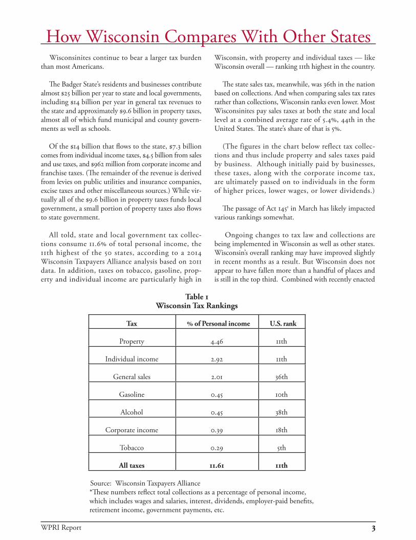
Wisconsinites continue to bear a larger tax burden than most Americans.

The Badger State’s residents and businesses contribute almost $25 billion per year to state and local governments, including $14 billion per year in general tax revenues to the state and approximately $9.6 billion in property taxes, almost all of which fund municipal and county govern-ments as well as schools.

Of the $14 billion that flows to the state, $7.3 billion comes from individual income taxes, $4.5 billion from sales and use taxes, and $962 million from corporate income and franchise taxes. (The remainder of the revenue is derived from levies on public utilities and insurance companies, excise taxes and other miscellaneous sources.) While vir-tually all of the $9.6 billion in property taxes funds local government, a small portion of property taxes also flows to state government.

All told, state and local government tax collec-tions consume 11.6% of total personal income, the 11th highest of the 50 states, according to a 2014 Wisconsin Taxpayers Alliance analysis based on 2011 data. In addition, taxes on tobacco, gasoline, prop-erty and individual income are particularly high in

How Wisconsin Compares With Other States

Wisconsin, with property and individual taxes — like Wisconsin overall — ranking 11th highest in the country.

The state sales tax, meanwhile, was 36th in the nation based on collections. And when comparing sales tax rates rather than collections, Wisconsin ranks even lower. Most Wisconsinites pay sales taxes at both the state and local level at a combined average rate of 5.4%, 44th in the United States. The state’s share of that is 5%.

(The figures in the chart below reflect tax collec-tions and thus include property and sales taxes paid by business. Although initially paid by businesses, these taxes, along with the corporate income tax, are ultimately passed on to individuals in the form of higher prices, lower wages, or lower dividends.) The passage of Act 1451 in March has likely impacted various rankings somewhat.

Ongoing changes to tax law and collections are being implemented in Wisconsin as well as other states. Wisconsin’s overall ranking may have improved slightly in recent months as a result. But Wisconsin does not appear to have fallen more than a handful of places and is still in the top third. Combined with recently enacted

Tax % of Personal income U.S. rank

Property 4.46 11th

Individual income 2.92 11th

General sales 2.01 36th

Gasoline 0.45 10th

Alcohol 0.45 38th

Corporate income 0.39 18th

Tobacco 0.29 5th

All taxes 11.61 11th

Source: Wisconsin Taxpayers Alliance *These numbers reflect total collections as a percentage of personal income, which includes wages and salaries, interest, dividends, employer-paid benefits, retirement income, government payments, etc.

Table 1Wisconsin Tax Rankings

4 WPRI Report

cuts, the largest tax reductions modeled for WPRI would bring Wisconsin closer to, though still slightly higher than, the average for all U.S. states.

Wisconsin has not conducted a comprehensive tax-impact study for more than a decade. But outside analyses indicate that the system remains progressive overall. And it will continue to be so even with recent changes under Act 145. In other words, low earners pay less in Wisconsin than their counterparts in most other states. High earn-ers pay more. According to the Minnesota Center for Fiscal Analysis, Wisconsin’s income tax was the 10th most progressive in 2010. A 2009 study by the Institute on Taxation and Economic Policy showed Wisconsin’s total state-local tax system to be ninth most progressive by its measure (ratio of tax burden of the bottom 20% to the top 1%). Although those data are relatively old, recent tax law changes may have made the system even more progressive.

One of the questions this state must address is whether the relative progressivity of its tax system, which is advan-tageous in the near-term to some individuals at the lower end of the economic spectrum but is the product of tax choices that harm Wisconsin’s long-term potential and productivity, can be retained in a way more aligned with the realities and opportunities of the modern economy.

WPRI Report 5

The Economics of State TaxesThe Fiscal Policy Test

Competition between states and foreign nations for new capital investment is one of the main drivers of tax reform.

Such investment takes many forms: business purchases or construction of nonresidential buildings, such as factories and offices; purchases of new equipment (for example, laptop computers and metal-working machines); and software, (such as Microsoft Office or Adobe Reader). Improving the business climate, specifically by raising the return on this sort of capital investment, is one of the keys to remaining competitive and driving economic development.

This is no secret. Across the United States, a variety of state-level tax reforms have been adopted with this in mind over the past 20 years, including tax and expendi-ture limitations and targeted tax cuts. Some states have considered tax swaps — or the substitution of one tax for another that is not as economically harmful. Some have earmarked new taxes for education and transportation with the belief that human capital and infrastructure investment enable growth.

With 21st century technology driving the restructur-ing of state economies, the transition to tax reform is difficult but necessary. For example, because of the rise of e-commerce and the decline of bricks-and-mortar retailers, state governments are seeking to tax Internet sales in order to recover “lost” revenues. The increasing use of electric vehicles and hybrids, modest today but expected to rise with environmental concerns, will mean that state governments can no longer rely on per-gallon gasoline taxes to maintain and build highways, roads and bridges. With the help of technology, states may turn to miles-traveled metering, higher fees or tolls.

Much attention, meanwhile, has been placed recently on the distortions faced by firms with profits from overseas. An emerging body of evidence suggests that tax consid-erations cannot be discounted in a global environment where capital is far more mobile than in the past.2 Firms defer bringing back profits from their multinational subsidiaries because of high U.S. corporate tax rates, thus leaving working capital out of reach. And then states present another level of corporate taxation.

The bottom line: States interested in economic growth cannot rely on a 20th century tax system that leans heavily on property taxes and individual and corporate income taxes. States that limit themselves to a light touch on taxes

believe justifiably that they will be rewarded with jobs and economic development.

Whatever new instruments of taxation are chosen, policy must be based on five basic principles: revenue-raising ability, neutrality, equity, ease of administration and accountability.3 Unfortunately, public finance economists who, in their wisdom, advise against both the opaque exemptions and the targeted tax incentives that pander to special interests are muted by short-sighted political pres-sures. A good tax system introduces a sense of certainty that engenders business confidence and taxpayer fidelity. Any such reform in Wisconsin should follow these principles.

Income Tax Considerations

Most states impose individual income taxes. States without them — Alaska, Florida, Nevada, New Hampshire, South Dakota, Texas, Washington and Wyoming — rely on other sources for revenue.4 Six states have no corpo-rate income tax: Nevada, Ohio, South Dakota, Texas, Washington and Wyoming.

In most states, however, income taxes remain a major source of revenue. Supporters of income taxes — both proportional and progressive — suggest that income taxes are more closely aligned with ability to pay, a long-standing objective of tax policy. Yet income taxes, both individual and corporate, distort decisions to work, save and invest and therefore threaten a state’s ability to com-pete for residents and businesses. By penalizing saving and diminishing incentives to work, the income tax shrinks employment, investment, production, productivity, and future well-being.

There are other negatives as well. The portion of the income tax levied on capital gains fluctuates along with the stock market, which makes such collections less pre-dictable. Taxpayer exemptions and deductions readily enacted by legislatures continually erode the tax base. Compliance costs, including time to complete tax forms, and the double taxation of investment income are among the reasons income taxes are less efficient than taxes on consumption.

There can be no principled debate over the question of whether discrimination against savers is per se an unattractive feature of the income tax. By any standard, this discrimination is not only inequitable but also has negative effects on economic activity. By penalizing sav-ing, the income tax shrinks investment and hence future production, productivity and well-being.

6 WPRI Report

Property Tax Considerations

Wisconsin property taxes provide the vast majority of tax revenues for local government and a very small amount of revenue for state government. But property taxes, particularly when levied on business property, can be economically harmful. The imposition of a business property tax leads to a reduction in the after-tax return derived from capital investments and creates a powerful disincentive for business owners inside the state to invest in their enterprises. Investment projects that would have been profitable enough to justify the investment without the presence of a high business property tax become less profitable on an after-tax basis. Capital investment in structures, as well as the employment and output that accompanies it, decreases.

Residential property taxes cannot be as clearly traced to income-producing activity such as earnings from either labor or capital. Partially due to this discon-nect, residential property taxes remain very unpopular. Sales and Consumption Tax Considerations

A sales or consumption tax does not have some of the negative features of income and business property taxes. Consumption taxes promote savings and investment, which are crucial to building a state’s capital stock and growth.5

Moreover, income and consumption taxes differ with respect to production and consumption relative to neigh-boring taxing jurisdictions, especially at the state level. An income tax that falls on capital and labor raises the cost of production for goods and services regardless of the location of the final sales, in-state or out-of-state. The higher cost reduces investment, employment and, ultimately, economic growth.

However, a consumption tax only taxes goods and services that are sold within the state’s borders. Therefore, goods and services that are produced in-state and sold out-of-state are free of taxation, making them more competitive on national markets. By freeing labor and capital from taxation, a consumption tax provides a pow-erful incentive for firms to locate production in the state

irrespective of where the final sales take place. In other words, a consumption tax rewards exports and penalizes imports. The higher levels of in-state production boost investment, employment and economic growth at the expense of current consumption of goods and services.

While Wisconsin’s sales tax rate is low in comparison to elsewhere, the state has limited ability to increase it without harmful consequences. There is, however, an alternative: broadening the sales tax base. In other words, there are numerous types of purchases that have never been subject to a sales tax in Wisconsin, or that have been exempted — a fact that has narrowed the tax base. By broadening the base, the state could increase revenue collections without having to raise the rate. Public finance experts generally prefer a broad base and low rate to a narrow base and higher rate.

As is the case with much of Wisconsin’s tax system and that of many other states, state sales and use taxes were built for a different economic era. In general, they were adopted during a time when the U.S. economy was largely goods-based and the taxes followed suit. Today the U.S. economy is more service-oriented. According to the U.S. Census, service industries account for 68% of U.S. gross domestic product and four out of five U.S. jobs.6 Most states have not reformed their sales tax laws to account for this fundamental change in the composition of the U.S. economy, and Wisconsin is no exception.

Wisconsin currently exempts a long list of goods from sales and use taxes. According to the most recent report from the Department of Revenue, the state specifically exempts goods and services that would have generated almost $4.7 billion in state tax revenue in fiscal year 2013.

Our objective here is to use our customized econometric model for Wisconsin, WI-STAMP, to determine the effects of various types of tax changes, including consumption taxes with a broadened base, at the state level.

WPRI Report 7

Brief Explanation of the WI-STAMP ModelThe Beacon Hill Institute’s Wisconsin State Tax Analysis

Modeling program (WI-STAMP) is a dynamic model that captures the effects of tax rate changes on economic activ-ity. Using WI-STAMP, we provide estimates of the effects of changes in state tax law on job creation, investment, real disposable income and state tax revenues.

Static estimates assume that there is no change in underlying economic activity in response to a change in tax law. For example, a static estimate of a cut in the sales tax, say from 5% to 4%, would expect revenues to fall by 20%.

A dynamic estimate would show a smaller drop in revenue because it would capture the positive effects on the tax base of freeing up more money through tax cuts and growing the economy. In other words, as a result of lower taxes, businesses would have more money to make profitable investments in Wisconsin, thus increasing employment, incomes, retail sales and, in turn, tax col-lections. One of the principal purposes of STAMP is to capture such dynamic effects.

While the increased economic activity would mitigate the lost revenue from the tax, it would not replace all of the lost revenue from the tax cuts. In other words, the STAMP model would not show that the tax cuts paid for themselves.

A further synopsis of the WI-STAMP methodology is contained in the appendix of this report and an even more detailed and complete explanation is attached to the digital version at www.wpri.org.

Generally speaking, the WI-STAMP model differenti-ates between the impacts of different sorts of taxes on job creation, investment, real disposable income and state tax revenues. It divides taxes into numerous categories, includ-ing so-called “factor taxes” on factors of production (such as labor and capital), sales and excise taxes, household taxes (such as the residential property tax and license fees) and income taxes. The model accounts for how different tax mixes and levels impact each area of economic activity, and it helps determine the optimum taxation strategy for long-term economic prosperity.

The Beacon Hill Institute entered the changes for each option into WI-STAMP and compared the results with the baseline situation to produce our estimate of the fis-cal and economic impact of such tax changes. We report the cumulative changes that would occur in 2018 as the result of a tax change in comparison to the baseline data in 2018 in the absence of the tax change. For example, if the Wisconsin economy were to create 10,000 jobs in 2018 without the tax change and we report that the tax change would create 10,000 jobs, then the economy would create 20,000 in 2018 under the tax change.

Beacon Hill modeled a variety of potential tax changes. The first category involves cuts to the individual and cor-porate income taxes and property taxes. We also examined revenue-neutral scenarios wherein cuts to individual and corporate income taxes and to both residential and business property taxes were offset by broadening the sales tax base.

8 WPRI Report

Tax-Cut ScenariosWisconsin has enacted significant tax cuts in recent

years, but further cuts would make the state even more competitive and more prosperous in the long term, accord-ing to economic modeling.

Beacon Hill modeled cuts to two different taxes cur-rently on the books in Wisconsin. The first option in Table 2 below analyzes a hypothetical individual income tax cut of 10% and a reduction of the corporate income tax rate to what would be a new top individual income tax rate of 6.885%.

The second option models the impact of reducing prop-erty taxes by a total of $280 million. This would include elimination of the only portion of property taxes — $80 million worth — that currently funds state (rather than local) government. It would also further reduce property taxes that fund technical colleges by $200 million, a cut that would come on top of a similar reduction made in the last budget cycle.

Under both scenarios, the state would benefit from both new jobs and increased investment. Job growth would be more significant, 11,300 private-sector jobs and a net job increase of 8,470, under the reduction of income taxes in Scenario 1. Investment would be slightly greater under the second scenario involving property tax cuts.

Scenario 1 Reduce the individual income tax by 10% and make the cor-

porate income tax rate equal to the new top individual income

tax rate of 6.885%.

Scenario 2Eliminate the state property tax ($80 million) and reduce the technical col-lege operating levy by $200 million.

Private Employment 11,300 2,260

Government employment -2,830 -1,930

Net employment 8,470 330

Investment $(m) 303 341

Real disposable income $(m) 1,155 265

State revenue loss $(m) -918 -241

Table 2 Tax-Cut Impacts by 2018

The state would experience a reduction of tax revenue under both scenarios, including $918 million under Scenario 1. However, taxpayers would be richer. Real disposable income would increase by more than $1.1 billion by fiscal 2018. In other words, real disposable income in Wisconsin would increase dramatically under individual income and corporate income tax cuts, and it would exceed the amount the state would lose in revenue. The result would be increased working, saving and spending, increased sales tax revenue and increased tax revenue from both wage and business growth.

Similarly, tax cuts and the elimination of the small portion of property taxes that funds state — rather than local — government would result in a reduction of revenue. While that would pose challenges, the money used to pay such taxes does not disappear from the state economy. Government services would need to be cut at the local or state level, which would lead to lower levels of government spending and/or employment. The WI-STAMP model accounts for this negative impact of lower government revenues, which diminishes the total economic impact of tax cuts. Nevertheless, the reduction in income and property taxes would provide a boost to the state’s private economy, leading to an increase in private employment, disposable income and investment, and to long-term net economic gain.

WPRI Report 9

Background

The debate over how large government — and its spending — should be is one of the essential conflicts in a democracy. Debate over the amount of revenue needed to fulfill the obligations of government is one thing. But the question of how government raises that revenue — and which taxes are least harmful to economic growth and prosperity — is another.

Today, that debate is often overshadowed by arguments between factions that will — no matter what the size of government — always reflexively argue either that taxes must be cut so individuals can keep more of their hard-earned money or that they must unceasingly be raised, used for government services and redistributed.

This section of the paper assumes that the current level of total funding, whether due to the realities of politics or governance, will continue to prevail. Any loss of revenue to government resulting from a cut in one tax will, within the WI-STAMP model, necessitate an increase of revenue from another source. Tax reformers, ergo, must balance the varied instruments of sales, income and corporate taxes, as well as user fees, in order to best enable citizens to thrive and prosper.

One of the ways Wisconsin can do this within a revenue-neutral environment is through fresh reconsideration of its overemphasis on property and income taxes and its relatively restrained current use of sales taxes.

As noted, consumption taxes are generally more eco-nomically efficient than other taxes — though not always or in all ways. Results will vary depending on how broad the tax base is.

Broadening the Base Versus Raising the Rate

The economic impacts of sales taxes are highly sensitive to the exact nature of the tax and the extent of exemptions.

Modeling reveals that the economic results of simply raising the rate on Wisconsin’s sales tax as it is currently constituted are mixed and, in some instances, minimal or negative. (The results of various rate-increase scenarios modeled by the Beacon Hill Institute are contained in the Appendix.)

There is an alternative to merely raising rates, however. Beacon Hill also modeled tax swaps involving a new, theoretical sales tax with a much broader base.

There are a host of ways to include more items in the sales tax base. Table 3 lists in declining value-order some of the leading items that have either been exempted from or never taxed by the Wisconsin sales tax. These are included in the hypothetical broad-base sales tax modeled by Beacon Hill. There are some other current exemptions built into Wisconsin tax law — mainly exemptions for health care services — that remain exempt in the theoretical scenario.

Of course, choice of what to tax or not to tax is a politi-cal decision, and legislatures have a long-demonstrated preference for granting exemptions to selected groups, a move that distorts market efficiency and eventually increases tax rates for all.

The purpose of the simulated changes outlined in the following section is to demonstrate that a broad-base sales tax can (1) keep rates lower than they would be otherwise and (2) have positive economic benefits for the state, especially when traded for historically high income and property taxes.

Higher-income households consume more goods and use more services – such as health clubs and legal, accounting and interior design work – than lower income households and will be impacted by a broadened sales tax base.

Taxing items such as food or motor fuel, on the other hand, inevitably generates claims of tax inequity. That problem can be easily overcome by providing low- and moderate-income households with a refundable, income tax credit to cover purchase of basic goods and services. In terms of who is and isn’t taxed, the credit approach is far more efficient in directing tax relief to those most in need than a total sales tax exemption. It is an approach that has served Wisconsin exceeding well since the 1960s. Through the well-established Homestead refundable tax credit, the state has long targeted property tax relief to low-income households with high property taxes.

Revenue-Neutral Tax Swaps Involving a Broadened Sales Tax Base

10 WPRI Report

Table 3 Items Included in the Sales Tax Base Expansion Scenarios

Good or Service 2012 $

Motor fuels 595,900,000

Food 536,900,000

Labor input into construction 499,400,000

Legal services 119,600,000

Fuel/Electricity for residential use 117,600,000

Vehicle trade-ins 97,100,000

Architecture/engineering services 83,800,000

Accounting services 51,000,000

Repair of real property 32,200,000

Sewer services 32,100,000

Water sold through mains 23,900,000

Commissions to real estate brokers 23,900,000

Beauty/barber 23,100,000

Veterinarian services 21,200,000

Bottled water 19,500,000

Health Clubs 17,000,000

Newspapers and magazines 14,500,000

Funeral services 12,600,000

Meals furnished by higher education 6,100,000

Admission to educational events 5,000,000

Caskets and burial vaults 4,800,000

Disinfecting/extermination services 3,300,000

Tax preparation services 2,100,000

Interior design 1,900,000

WPRI Report 11

The economic advantage of broadening the base by, for instance, including the items specified in the chart above versus simply raising the rate is clear.

Table 4 below illustrates this by juxtaposing two very similar scenarios. Both scenarios eliminate the portion of the property tax that funds state, rather than local, government. Both remove funding for tech schools and counties from the local property tax levy. Both eliminate the personal property tax. They differ only in how they treat the sales tax. One scenario simply raises the rate on the sales tax as currently constituted. The other, which broadens the base, has a considerably more positive impact.

Broadening the base, for example, would create 6,720 jobs by 2018, whereas raising the rate would cost 1,660 jobs, a difference of 8,380 jobs or roughly the population of Rice Lake, Delavan or Ashland. As the table shows, broadening the base is also much more advantageous in other ways, including a difference of well more than $400 million in impact on state revenue.

Economic theory is clear on the advantages of a broad-ened base. Under the sales tax base expansion scenarios, the new sales tax burden is spread across many industries and therefore the increase produces less economic distor-tion7 to any one industry in particular. In other words, a sales tax rate increase would place a significantly larger burden on those industries already currently facing the tax. Firms in these industries would face a much higher marginal increase — one that is economically harmful — than under the base-broadening scenario.

Currently, the retail and wholesale sectors employ the most workers of any industry in the state, almost 400,000,

or 16% of total state employment. Were the sales tax rate simply increased, the burden would fall on these labor-intensive sectors disproportionally, causing more damage to employment than if spread out to other sec-tors. Conversely, under the expanded base scenarios, the industries that bear the burden of the current sales tax regime, particularly retail and wholesale sectors, do not experience a tax increase and therefore escape any new burden. This provides an economic boost to those industries that partially offsets the losses faced by those industries subject to the base expansion.

The base expansion scenarios, in other words, would expand the sales tax to industries that do not use labor as intensively as the retail and wholesale industries. For example, the food, transportation, utility and real estate sectors would be subject to the sales tax base expansion and employ only about 250,000 workers combined.

Looked at another way, labor produces more than 71% of income to Wisconsin’s households. Return on capital provides only 16%, and government transfers provide the rest. Changes to the relative tax burden between industries can cause different impacts on income. For example, when taxes increase on industries that use more labor, such as a tax increase on the retail and wholesale industries, there is a larger negative effect on incomes than when taxes are raised on capital-intensive industries.

Establishing a sales tax regime with few or no exemp-tions for taxes levied upon goods and services is the key to effective reform, and a crucial tenet of sound tax policy.

Increase the sales tax rate Broaden the sales tax base

Sales tax rate 8.10% 5.0%

Private employment -1,660 6,720

Investment $(m) 2,600 2,693

Real disposable income $(m) -984 358

State revenue impact $(m) -39 378

Table 4 Impacts of Revenue-Neutral Tax Swaps by 2018: Rate Hike Versus Base Broadening

12 WPRI Report

Results

Table 5 reveals significant, positive impacts to pri-vate-sector employment, investment and real disposable income that would result from broadening the sales tax base and lowering other taxes in a revenue-neutral situa-tion, and often with a lower or unchanged sales tax rate. Under Scenario 1 where all income taxes would be elimi-nated coupled with a broad sales tax of 9.5%, WI-STAMP found that private employment would increase dramati-cally, by 33,870 jobs, and real disposable income would increase by over $2.3 billion. This scenario produces the largest positive impact on employment and, due to the elimination of the personal income tax, the largest increase in disposable income. Eliminating the personal income tax simultaneously increases workers’ take-home pay and reduces employers’ labor costs.

Eliminating the state property tax and unhinging tech school funding from local property tax levies (Scenario 2) would result in 8,230 jobs — and a significantly lower rate. This scenario results in relatively modest changes in employment, income and investment.

Scenario 3 — the same one contained in Table 4 illus-trating the difference between using a sales tax rate increase

Scenario 1 Eliminate all income taxes,

both corporate and personal, and replace

with new sales tax structure.

Scenario 2 Eliminate the

small state-levied property tax

and remove all funding for tech schools from the local property tax levy. Replace with

a sales tax with a much broader

base.

Scenario 3 Eliminate the

state property tax. Remove funding

for tech schools and counties from the local property tax

levy. Also, eliminate the personal prop-erty tax. Replace

with sales tax with broader base.

Scenario 4 Cut the individ-ual income tax

by $730 million. Cut the prop-

erty tax by $1.11 billion. Use new sales tax base to cover the loss.

Sales Tax Rate 9.5% 3.75% 5.0% 4.475%

Private employment 33,870 8,230 6,720 10,580

Investment $(m) 893 825 2,693 948

Real disposable income $(m) 2,310 885 358 892

State revenue loss $(m) -47 -23 378 -21

and broadening the base — has a $2.6 billion positive impact on investment and no change in the rate. The leap in investment, combined with a sales tax base that is forecast to grow faster than the property tax base, boosts revenues by $378 million in 2018.

Scenario 4 is, perhaps, the most interesting. It models a balancing of the tax mix so that income and property taxes are about average compared with the mixes in other states. This scenario calls for a cut in the individual income tax and property tax by $730 million and $1.1 billion respectively, and a broadened sales tax base that would make the changes essentially revenue-neutral. Jobs would increase by 10,580; investment would increase by $948 million; real disposable income would increase by $892 million — and Wisconsin would have a lower sales tax rate.

While Scenario 1 provides the largest boost to employment and Scenario 3 produces the largest increase in investment, Scenario 4 provides the most balanced increase between the two.

In sum, by altering the tax mix, Wisconsin could set itself up for substantial economic growth, lower the sales tax rate as well as income and property taxes, and lose very little tax revenue.

Impacts of Revenue-Neutral Exchange of Income and Property Taxes for Sales Tax with Broadened Base by 2018

Table 5

WPRI Report 13

ConclusionIn the 21st century, Wisconsin faces enormous com-

petitive pressures not only from other states but from nations across the globe.

The Badger State has made progress in cutting taxes in recent years but still taxes its citizens and businesses to a significantly higher degree than other states and areas with which it must compete.

Modeling shows that Wisconsin would benefit eco-nomically from cutting taxes and changing the tax mix by lowering taxes on income and capital and partially paying for the cuts with an expanded sales tax base. A move away from income taxation and toward consump-tion taxation would drive economic growth by lowering the cost of savings, the resource for investment in new business expansion. In addition, a lower tax burden on income would also lower the pretax cost of wages, provid-ing an incentive for businesses to locate employment and investment in Wisconsin.

The proposals evaluated by the WI-STAMP model, in sum, provide a strong argument for consumption taxes over income and other taxes. While all taxes have negative features, economic theory favors a broad-based consumption tax because it avoids taxing the products of one’s work and does not penalize investment the way some other taxes do.

To be sure, there are numerous ways to structure a broad-based consumption tax, including, for example, broadening of traditional sales taxes, value-added taxation and the use of gross-receipts taxes.

Some places such as Washington state used a broad-based, traditional sales tax. The combined state and local average sales tax rate in Washington State is the fourth highest in the country, according to Tax Foundation data from 2013, and that state also has a very broad base.

Value-added taxes are another option. In 2009, for instance, California’s Commission on the 21st Century Economy recommended reducing and simplifying the state’s individual income tax, eliminating the state’s cor-porate tax and general sales tax, and instead using what was essentially a value-added system to de facto broaden the sales tax base. Value-added taxes tax the value that a business adds to the production of products and services but can act as broad-based consumption taxes. Despite support from then Gov. Arnold Schwarzenegger, the commission’s recommendations gained little political trac-tion. Value-added taxation, if approached the right way, has gained some theoretical support across the political

spectrum. Part of the opposition in the past, however, has stemmed from fears that it will piggyback on top of other taxes instead of supplant them.

Meanwhile, other states such as Hawaii have enacted or considered what are sometimes referred to as “gross-receipts” taxes that, if structured the right way, can act like broad-based consumption taxes. Critics of such taxes often focus on how the tax “pyramids” on products as they move through the production process and results in a high effective tax rate on the final product. There are also concerns about taxation on businesses that fail to make a profit, and the “hidden nature of the tax.” The real harm from such taxes, some counter, comes from politically motivated exemptions that make them too narrow and less economically advantageous.

Some of these big-picture questions about how best to broaden the consumption tax base deserve further, in-depth analysis — as does the question of tax impacts. While there will be concern that expanding consumption taxes will make Wisconsin’s tax system less fair, refundable income tax credits to low-income taxpayers can be a vehicle to lessen the regressive nature of a consumption-based tax system and also enable long-term economic growth and global competitiveness.

For now, it is clear that Wisconsin would immediately benefit not just from lower income and property taxes but from a system that broadens and reforms the exist-ing sales tax as well. Policymakers should immediately consider these actions for a simple reason: If adopted by legislators, the changes would have a substantial impact on jobs, income and investment.

As with any change worth examining, reform would not be without near-term controversy and burden. But Wisconsin must look beyond today and into a future where each citizen and business would have the opportunity to benefit from more jobs, more investment and a brighter, more vibrant and prosperous economy.

14 WPRI Report

Scenario 1 Eliminate the small state-

levied property tax and remove all funding for

tech schools from the local property tax

levy.

Scenario 2 Eliminate the state property tax. Remove funding for tech schools

from the local property

tax levy and eliminate the

personal prop-erty tax.

Scenario 3 Cut the indi-

vidual income tax by $730 mil-

lion. Cut the property tax by

$1.11 billion.

New Sales Tax Rate 6% 6.3% 7.05%

Private employment -1,750 2,270 640

Investment $(m) 680 628 814

Real disposable income $(m) -380 -550 (464)

State revenue loss $(m) No change -15 (26)

Appendix

Table 6 Impacts of Revenue-Neutral Exchange of Income and Property Taxes for a

Sales Tax Rate Increase by 2018

property taxes. All of the scenarios result in large losses in disposable income, and very little positive (or negative) impact on the job market.

The following table presents four different scenarios, all involving an increased use of Wisconsin’s sales tax as currently constituted — i.e., higher sales tax rates and sales tax revenue — and concomitant cuts in income and/or

WPRI Report 15

places: household disposable income and disposable tax-able income. Thus, changing the residential property tax impacts the state economy through disposable income. A change in disposable income changes real private con-sumption, which, in turn, changes domestic demand, domestic supply and intermediate demand. The change in domestic supply triggers a change in factor demand and a higher level of production in the production function. The higher level of factor demand, without a change to the rental rates or the factors, causes a change in household income, which changes real disposable income, which in turn, changes private consumption, which changes domestic demand until the cycle begins again. However, the household taxes do not directly affect production by changing prices or the rental rates of labor and capital or the factor demand equations.

The sales and other excise taxes are treated as excise taxes that affect price levels in the industries on which they are levied. This directly feeds into the calculation of the consumer price index, real private consumption, value added and government income. Through its effect on the consumer price index, the sales tax indirectly affects real household disposable income, household purchases from out of state, the price investment by sector source and the price of value added.

The change in real private consumption causes a change in domestic demand, which, in turn, causes domestic supply to change to meet the portion of the change in domestic demand met by in-state suppliers. Intermediate demand also changes in response to the change in domestic supply.

The price change also affects the price of value added. The changes in domestic supply alter the right side of the factor-demand equation and effect a response in the demand for labor and capital. The change in factor demand enters the production function and either increases or decreases production. The change in factor demand also causes a subsequent change in factor income, which in turn changes household income. This changes real dis-posable income, which in turn, impinges upon private consumption, which changes domestic demand, where the cycle begins again.

Like the household taxes entered into the model, the excise taxes do not directly affect production by the rental rates of labor and capital or the factor-demand equations. However, since excise taxes do change the price level, they affect disposable income and value added, so they have a larger effect than the residential property tax. Generally, a replacement of residential property tax revenues with sales tax revenues will produce lower levels of economic activity, including employment and income.

MethodologyTo identify the economic effects of the tax discounts and

understand how they operate through a state’s economy, the Beacon Hill Institute customized its STAMP® (State Tax Analysis Modeling Program) model for Wisconsin (WI-STAMP).7 WI-STAMP is a five-year, dynamic, computable general equilibrium model that has been programmed to simulate changes in taxes, costs (general and sector-specific) and other economic inputs. As such, it provides a mathematical description of the economic relationships among producers, households, governments and the rest of the world.8

A CGE tax model is a computerized method of account-ing for the economic effects of tax policy changes. A CGE model is specified in terms of supply and demand for each economic variable included in the model, where the quantity supplied or demanded of each variable depends on the price of each variable. Tax policy changes are shown to affect economic activity through their effects on the prices of outputs and of the factors of production (prin-cipally, labor and capital) that enter into those outputs.

A CGE model is in “equilibrium,” in the sense that supply is assumed to equal demand for the individual markets in the model. For this to be true, prices are allowed to adjust within the model (i.e., they are “endogenous”). For instance, if the demand for labor rises while the sup-ply remains unchanged, then the wage rate must rise to bring the labor market into equilibrium. A CGE model quantifies this effect.

Finally, a CGE model is numerically specified (“com-putable”), which is to say it incorporates parameters that are believed to be descriptive of the actual relationships between quantities and prices. It produces estimates of changes in quantities (such as employment, the capital stock, gross state product and personal consumption expenditures) that result from changes in prices (such as the price of labor or the cost of capital) arising from changes in tax policy (such as the substitution of an income tax for a sales tax).

Because it consists of a large number of interrelated equations, a CGE model ordinarily requires the applica-tion of a nonlinear computational algorithm, typically some variation on Newton’s method. STAMP requires the development and application of a sophisticated computer program for the solution of its equations.

The WI-STAMP model handles different taxes in different ways.

The residential property tax is treated as a household tax and enters the STAMP model only in two other

16 WPRI Report

The business property and corporate income taxes are treated as factor taxes on capital in the STAMP model. These taxes enter the household gross income equation, factor-demand equation, gross investment by destination, government income and production-function equation. Changes to these taxes cause changes to the demand for capital mostly through the rental rate of capital. Lower taxes lead to a lower real rental rate of capital and thus a higher demand for capital investment. To a much lesser extent, the change in the rental rate of capital relative to the rental rate of labor makes capital more attractive to employ relative to labor, and there is a substitution effect between the two factors.

WPRI Report 17

About the AuthorsDavid G. Tuerck, Ph.D., is executive director of the Beacon Hill Institute for Public Policy Research at Suffolk

University, where he also serves as chairman and professor of economics. He holds a Ph.D. in economics from the University of Virginia and has written extensively on issues of taxation and public economics.

Paul Bachman, MSIE, is director of research at the Beacon Hill Institute. He manages the institute’s research proj-ects, including the development and deployment of the STAMP model. Mr. Bachman has authored research papers on state and national tax policy and on state labor policy. Each year, he produces the institute’s state revenue forecasts for the Massachusetts Legislature. He holds a master of science in international economics from Suffolk University.

Michael Head, MSEP, is a research economist at BHI. He holds a master of science in economic policy from Suffolk University.

Frank Conte, MS, is the director of communications and information systems at BHI. He holds a master of science in public affairs from the University of Massachusetts-Boston.

WPRI Report18 WPRI Report

1 As enacted, Act 145:

• reduces the state’s income tax rate on the bottom bracket from 4.4% to 4.0%, representing a $98 million cut;

• provides for tax credits to offset the state’s alternative minimum tax;

• cuts corporate taxes by allowing business to carry forward losses up to 20 years;

• adjusts withholding tables for most taxpayers, which will result in a reduction of income tax collections by $156.5 million in the current fiscal year and by $166.1 million in fiscal year 2015;

• alters income tax withholding rates, commencing in April 2014, so workers have less taken out of each paycheck (roughly $520 a year for a married couple now earning $80,000 a year);

• provides for property tax relief in the form of changes to levy limits applicable to technical college districts; and

• eliminates income tax rates for manufacturers. 2Richard B. McKenzie and Dwight R. Lee, Quicksilver Capital: How the Rapid Movement of Wealth Has Changed the World (New York: The Free Press, 1991.) 3David Brunori, State Tax Policy: A Political Perspective, (Washington, D.C.: Urban Institute Press, 2001), 13-29 4(New Hampshire and Tennessee do not tax wage income but tax dividend income instead.) 5Alan J. Auerbach, “The Choice between Income and Consumption Taxes: A Primer,” NBER Working Paper 12307. National Bureau of Economic Research (June 2006), 23, http://www.nber.org/papers/w12307. 6U.S. Census, Gross Domestic Product, http://www.census.gov/compendia/statab/cats/income_expenditures_poverty_wealth/gross_domestic_product_gdp.html. See also Bernard Baumohl, The Secrets of Economic Indicators (Upper Saddle, N.J.: FT Press, 2013), 134.

7For more details see http://www.beaconhill.org/STAMP_Web_Brochure/STAMP_IntroductionMS.html.

8For a clear introduction to CGE tax models, see John B. Shoven and John Whalley, “Applied General-Equilibrium Models of Taxation and International Trade: An Introduction and Survey,” Journal of Economic Literature 22 (September, 1984): 1008. Shoven and Whalley have also written a useful book on the practice of CGE modeling entitled Applying General Equilibrium (Cambridge, Mass.: Cambridge University Press, 1992). See also Roberta Piermartini and Robert Teh, Demystifying Modeling Methods for Trade Policy (Geneva, Switzerland: World Trade Organization, 2005) http://www.wto.org/english/res_e/booksp_e/discussion_papers10_e.pdf (accessed June 18, 2010).

Endnotes

TABLE OF CONTENTS

What is STAMP? ............................................................................................................ 2 Constructing a CGE model ............................................................................................. 4 Detailed Equations for STAMP .................................................................................... 11 Household Demand ....................................................................................................... 11 Labor Supply ................................................................................................................. 15 Migration....................................................................................................................... 15 The Behavior of Producers/Firms ................................................................................. 16 Trade with other States and Countries .......................................................................... 19 Investment ..................................................................................................................... 21 Government................................................................................................................... 23

Model Closure ............................................................................................................... 27 Objective Function ........................................................................................................ 31 Elasticity Assumptions for STAMP.............................................................................. 32 The Beacon Hill Institute STAMP Development Team ............................................... 39

TABLE OF TABLES

FIGURE 1. CIRCULAR FLOW DIAGRAM ........................................................................................................... 3 TABLE 1. GOVERNMENT SECTORS .................................................................................................................. 8 TABLE 2. INDUSTRY ELASTICITIES ................................................................................................................33 TABLE 3. HOUSEHOLD-RELATED ELASTICITIES ............................................................................................35

STAMP 2

What is STAMP?

STAMP is a comprehensive model of the state economy, designed to capture the principal effects

of city tax changes on that economy. STAMP is a five-year dynamic computable general

equilibrium (CGE) tax model. As such, it provides a mathematical description of the economic

relationships among producers, households, government and the rest of the world. It is general in

the sense that it takes all the important markets and flows into account. It is an equilibrium model

because it assumes that demand equals supply in every market (goods and services, labor and

capital); this is achieved by allowing prices to adjust within the model (i.e., prices are

endogenous). The model is computable because it can be used to generate numeric solutions to

concrete policy and tax changes, with the help of a computer. And it is a tax model because it

pays particular attention to identifying the role played by different taxes.1

We begin by distinguishing between producers and consumers. Consumers/households earn

income by supplying labor (wages and salaries) and capital (dividends and interest); they also

receive transfer payments such as pensions. They are assumed to maximize their utility, which

they do by using income to buy goods and services, pay taxes and save. Their spending decisions

are strongly influenced by the structure of prices they face; and the amount of labor that they are

willing to provide depends to a substantial degree on the wage rates that they face.

Producers/firms buy inputs (labor, capital and intermediate goods that are produced by other

firms) and transform them into outputs. Producers are assumed to maximize profits and are likely

to change their decisions about how much to buy or produce depending on the prices they face for

inputs and outputs.

In addition, there is a government sector that collects taxes and fees and provides services and

transfers. The rest-of-the world sector consists of the entire world outside of the state. The

relationships between these components are set out in the circular flow diagram shown in Figure

1.2 The arrows in the diagram represent flows of money (for instance, households purchase

1 For a clear introduction to CGE tax models, see John B. Shoven and John Whalley, “Applied General-Equilibrium Models of Taxation and International Trade: An Introduction and Survey,” Journal of

Economic Literature, XXII (September, 1984), 1008. Shoven and Whalley have also written a useful book on the practice of CGE modeling entitled Applying General Equilibrium (Cambridge: Cambridge University Press, 1992). 2 Based on a similar diagram in Berck et al., Dynamic Revenue Analysis for California.

STAMP 3

goods and services), and flows of goods and services (for instance, households supply their labor

to firms). The separate box for government shows the flows of funds to government in the form

of taxes, as well as government purchases of goods and services and government hiring of labor

and capital.

Figure 1. Circular Flow Diagram

Complex as it may seem, the diagram in Figure 1 is still too simple, because it lumps all

households into one group, and all firms into another. To provide further detail it is necessary to

create sectors; STAMP has 81 economic sectors. Each sector is an aggregate that groups together

segments of the economy. We separate households into seven income classes and firms into 27

industrial sectors. In addition, we distinguish between 30 types of taxes and funds (four at the

federal level, 13 at the state level, and 12 at the city level) and 13 categories of government

spending (two at the federal level, six at the state level, and five at the city level). To complete

the model, there are two factor sectors (labor, capital), an investment sector and a sector that

represents the rest of the world. The choice of sectors was dictated by the availability of suitably

disaggregated data (for households and firms), and the purposes of the model.

Sub-national models, such as STAMP, are similar in many ways to national and international

CGE models. However, they differ in a number of important respects, which are as follows:

STAMP 4

a. In a national model, most saving goes toward domestic investment; however, this need

not be true at the regional level. If citizens save more than they spend, then the excess

saving will leak out of the state.

b. The smaller the unit under consideration, the greater the importance of trade with the rest

of the world. This is an important consideration for state models.

c. Migration is likely to be larger and more responsive across cities and states than across

nations.

d. In sub-national models, taxes are interdependent. So, for instance, the amount of revenue

collected by the Federal personal income tax depends significantly on whether there is a

state or local income tax (which may be deducted from income before computing the

Federal tax).

e. Data are less available at the sub-national than national level. This explains why scores

of national CGE models have been built, but relatively few sub-national models.

Constructing a CGE model

The construction of a CGE model involves several steps. First, one needs to organize the data

needed by the model. STAMP starts with data for a single fiscal year, 2004, which we use as a

basis to develop a steady state path through fiscal year 2010 in the model. This steady state path

is attained by applying growth rates for investment, population, employment and inflation

throughout the time frame of the model. In STAMP, the investment growth rate is assumed to be

1.31%.3 The growth rate for population is assumed to be 1.7%.4 The inflation growth rate is

assumed to be 3.00%5. To attain a reasonable steady state path, the data for the base year, fiscal

year 2004, must be very detailed. Most of the data are organized into a Social Accounting Matrix

(SAM), which in this case consists of an 81 by 81 matrix that accounts for the main economic and

fiscal flows in the state.

The model also requires some additional information – for instance, data on employment and on

the structure of the Federal income tax – which are put in separate files. And the model requires

information on “elasticities;” these are the parameters, typically taken from the academic

literature, that measure the responsiveness of households to changes in prices and wages, and of

3 This figure is derived from taking the average nominal US gross domestic investment for the period 1929-2004 as published by the Bureau of Economic Analysis. 4 This figure is the Census projection for the period 2005-2010. 5 This figure is based on data obtained from the U.S. Bureau of Labor Statistics.

STAMP 5

firms to changes in input costs and output prices. These are set out in detail in Section 4 of this

report. The economy is assumed to be competitive, and to run at full employment (by which we

mean that there is no involuntary unemployment).

Second, the model needs to be specified in detail; the next section of this report sets out details of

the model that we constructed, along with some comments explaining the choices made at each

step.

The third step is to program the model. For this we used the specialized GAMS (General

Algebraic Modeling System) software. In order to make the model easier to use, we also

developed an interface in Microsoft Excel. This allows the user to enter tax changes on an Excel

spreadsheet, click the “Estimate CGE” button, and read the key output on the same spreadsheet;

the heavy-duty computing occurs in the background.

Before use, the model must be calibrated. Calibration consists of running the model – i.e., asking

it to solve for all the variables in such a way as to maximize (and minimize!) total personal

income.6 The results for the base year are checked to see that they correspond with the actual

values of the variables in the SAM. Once the model reproduces the base year values, it is

considered calibrated. Calibration is an important step, as it is essentially a way of checking that

the model is working properly.

After it has been calibrated, the model is ready to be used to quantify tax change effects. The

procedure is straightforward: specify a new tax rate (or change in the tax), run the model, and

compare the new results with the steady state ones. At this point it is also possible to test the

sensitivity of the results to different assumptions – such as the values of elasticities – that are

incorporated into the model. It is worth stressing that STAMP is a policy model and not a

forecasting model; in other words it is designed to answer “what if?” questions, not to estimate

what is actually expected to occur in coming years.

6 The choice of variable to maximize has no substantive importance, and is a device for getting the model to solve.

STAMP 6

THE STAMP: THE MODEL OUTLINED

Organizing the Data

The starting point in building a CGE model is to determine the degree of detail that is desired and

to organize the collected data into the useful format of a Social Accounting Matrix (SAM) for the

base year. The SAM that we developed is an 81 by 81 matrix. Each of the 5,929 cells in the

matrix represents the dollar value of a flow from one sector of the economy to another – for

instance, purchases of business services by the utilities sector, or labor earnings flowing to

middle-income households. Reading along a row, one finds the payments received by that sector;

reading down a column, one sees the payments made by that sector. The SAM is balanced, which

means that the sum of the entries in any given row equals the sum of the entries in the

corresponding column. Thus, for instance, the revenue received by utilities must equal spending

by that sector, so that all incoming and outgoing funds are completely accounted for.

For STAMP, we distinguish 27 industrial sectors, two factors (labor and capital), seven household

categories, an investment sector, 43 government sectors (26 for taxes, 13 for spending, four

government funds) and a sector for the rest of the world. In sectoring the economy we sought to

strike a balance between providing a high level of detail (especially on the tax side) and keeping

the model to a manageable size. An additional limitation is that the lack of finely disaggregated

data limits the degree of detail that is possible. Data availability also determined some of the

choices we made; for instance, it is possible to get a breakdown of households into seven income

categories (see below for further details), and while we might have preferred a different set of

categories, we were constrained by the nature of the data available.

Industrial sectors

Although data for 49 sectors were actually available from the Bureau of Economic Analysis,

STAMP contains only 27 industrial sectors. This is because some sectors were too small to merit

separate attention. In these cases, we combined some industries, such as textiles and apparel. In

other cases, there were no matching employment figures, and so it was easier to work with

aggregates.

STAMP 7

Factor Sectors

We distinguish between two factors, labor and capital (which includes land). Businesses pay

wages and salaries to labor, and they generate profits. These are then distributed to household

owners as factor income.

Household Sectors

In STAMP, households receive wages, capital income and transfers and they use this income to

buy goods and services to pay taxes; and to save. We distinguish seven household sectors, which

group households by their levels of income. Expenditure data are available for households in

each of these categories, which make it relatively straightforward to work with this structure.

One purpose of this disaggregation of households is to allow one to trace the distributive effect of

tax changes and another one is to allow different groups to have different levels of sensitivity to

labor market conditions.

Investment Sector

There is one investment/savings sector. Households save, both directly out of their cash incomes,

and indirectly because they own shares in businesses that save and reinvest profits. The

government also saves and invests. Information is available from the Bureau of Economic

Analysis (BEA) on the pattern of gross investment by destination (i.e., how much gross

investment went into adding to the stock of capital in utilities, in industry, and so on). We have

constructed measures of the capital stock in each sector, and by applying published depreciation

rates and adding gross investment, arrived at the capital stock in the subsequent period. This

permits the model to track the expansion of the economy over time. The BEA has also produced

a matrix, built for the U.S. for 1997, which maps investment by destination with investment by

source. This mapping allows one to determine, for example, how much of the investment

destined for utilities is spent on purchasing goods and services from the construction sector and

the transport sector. Thus if investment rises, it is possible to identify which sectors would face

an expansion in the demand for their output.

STAMP 8

Government Sectors

STAMP was designed primarily to analyze the effects of major changes in the structure of state

taxes, and so we have paid particular attention to providing sufficient detail for government

transactions. The sectoring is summarized below in Table 1.

Table 1. Government Sectors

Federal Government Receipts

USSSTX Social Security (OASDI and MEDICARE)

Receives payments from employers and households; pays out transfers to households.

USPITX Federal Personal Income Tax Receives payments from households, which are put into the Federal normal spending account.

USCITX Federal Corporation Income Tax Receives payments from corporations and channels them into the Federal normal spending account.

USOTTX Other Federal Taxes Includes excises on motor fuel, alcohol, and tobacco; estate and gift taxes. Also funneled into the Federal normal spending account.

Federal Government Expenditure

USNOND Federal Normal Spending Federal government purchases goods and services, hires labor, and transfers money to and to Federal defense fund.

USDEFF Federal Defense Spending Purchases goods and services, and pays labor for military purposes.

State Government Receipts

STCITX State Business and Occupation Tax Revenues go into state general fund.

STSATX State Sales Tax Revenues go into state general fund.

STIHTX State Inheritance Tax Revenues go into state general fund.

STINTX State Insurance Tax Revenues go into state general fund.

STFUTX State Taxes on Motor Fuels Revenues go into state special fund and highway fund.

STOGTX State Public Utility Tax Revenues go into state general fund.

STALTX State Alcohol Beverage Taxes Revenues go into state general fund.

STTCTX State Tax on Cigarettes and Tobacco Revenues go into state general fund.

STPRTX State Property Tax Revenues go into state general fund.

STOTTX State Other Taxes Revenues go into state general fund and Other funds.

STMOTX State Motor Vehicle Fee Revenues go into state general fund.

STWKTX State Unemployment Insurance Tax Sector combines workers unemployment funds. Receipts go into proprietary fund.

STFEES State Fees, License Permits and Other Revenue

Revenues go into all funds.

STGENF State General Fund An accounting device. Tax revenue is channeled into this fund before being distributed to other uses.

STAMP 9

STSPCF State Special Funds An accounting device. Tax revenue is channeled into this fund before being distributed to other uses.

State Government Expenditure

STGGSP State General Spending General government spending.

STEDUC State Spending on Education Mainly purchases of goods and services and labor in the higher education sector.

STHELT State Spending on Health & Welfare Buys some services; mainly transfers funds to local health spending fund.

STPBSF Public Safety Public safety and fire departments spending.

STTRAN State Spending on Transport Mainly buys engineering services and construction.

STOTHS State Other Spending Miscellaneous other spending by the state on labor, goods and services.

Local Government Receipts

LOPRTX Local Tax on Residential Property Revenues go into the local general fund.

LOPBTX Local Tax on Business Property Revenues go into the local general fund.

LOOTRE Local Taxes Other Revenues go to the local general fund.

LOCHAR Local Public Service Charge and Fees Revenues go to all three funds (general, capital projects and other)

Local Government Expenditure

LOEDUC Local Spending on Education Purchases goods and services and (mainly) pays teacher salaries.

LOHELT Local Spending on Health & Welfare Purchases goods and services and pays labor; large transfers to the poorest category of households.

LOPBSF Local Public Safety Public safety and fire departments local spending.

LOTRAN Local Spending on Local Transportation Mainly buys engineering services and construction.

LOOTHS Local Other Spending Includes spending on police and firefighters, road repair, and miscellaneous local government services.

The government collects revenue from taxes and fees. Specific tax categories at the state level

included in the model are: sales and use, cigarettes and tobacco, mortgage recording, corporate

and personal incomes, and taxes both on residential and commercial properties. The rest of the

state taxes are grouped into a residual category (other local taxes).

The revenues from the taxes go to either the general fund, the capital projects fund or to other

funds, or a combination of them. Funds then allocate the money into the five spending

categories: education, health and welfare, transportation, public safety or others.

STAMP 10

Rest of the World

To complete the model, we have included a sector for the rest of the world (ROWSCT). This

refers to the world outside of , i.e., the rest of the United States and other countries. Information

on flows between the state and the rest of the world is difficult to piece together, and is an area

where considerable professional judgment was required.

STAMP 11

5. STAMP: THE MODEL IN DETAIL

This section of the report explains the STAMP model in detail. First, we introduce each equation,

providing some context and a short description. Then we present each equation in mathematical

form, provide information on the sources of data used, and summarize the elasticity assumptions

used in the model.

Detailed Equations for STAMP

STAMP is a dynamic CGE model which assumes a steady state growth path. Absent from any

“shocks”, the economy is assumed to remain on this path. If the economy experiences a shock,

such as a tax change, the economy will diverge from this steady state path and eventually turn

onto a new path. The size and length of the divergence will depend on the size of the shock to the

economy. Below we set out the equations used in STAMP and the assumptions inherent in them.

Household Demand

Households are assumed to maximize their well being (“utility”) by picking baskets of goods and

services, subject to their budget constraints. The key set of equations in this section is labeled

Private Consumption, and consists of a set of demand functions. These demand functions, based

on a Cobb-Douglas utility function, take on the simple form,

,,

* , 1,..., ; 1,...t

t i i

t i

IX i n t n

P ,

where Xt,i is the quantity demanded of good i at time t, Pt,i is the price of good i at time t, It is

income at time t, and i are parameters that measure the share of income that is devoted to good i.

This is the simplest specification that is theoretically satisfactory: it is additive (so spending

equals income less taxes less saving), has downward-sloping demand (ensuring that when the

price of a good rises, the quantity demanded falls), is zero degree homogeneous in prices and

income (so that if prices and incomes were to double, the quantity demanded would not change),

and meets the technical requirement of symmetry of the Slutsky matrix. More complex

formulations are possible, but there is a lack of reliable data on the elasticity parameters that

would be needed in such cases.

Household Gross Factor Income

STAMP 12

Comments: The gross income of households in each of the seven groups (indexed by h in the

set H) is found by first summing factor income (yf) from labor and capital,

subtracting the social security contributions paid by employees, and then

allocating the total to each group on the basis of fixed shares. Factor payments

are allocated to each household group using the same fixed shares as were found

in the base year.

Eq. 1. FfHhTtFFPya

ay

Ff GFg

fh

fgtfft

Hh

w

htfh

w

htfh

ht

,,11 ,,,,,

,,,

Description: Household income is the sum of income from each factor (labor and capital) less

factor taxes, distributed by household groups according to their share of total.

Data: The information on earnings for each household group comes from IMPLAN (an

economic impact modeling system which allows users to perform in-depth

regional analysis. See http://www.implan.com for more details).

Household Disposable Income

Comments: Disposable household income is gross income, less taxes on household income

and property (mainly personal income tax (USPITX, STPITX) and residential

property tax (LOPRTX)), plus transfer payments (such as social security and

unemployment benefits).

Eq. 2. , , , , , , , , , , , ,d hh h hh n pc

t h t h t g h t h t g h t h hg t h t h g

g GI g GH g G

y y t a a w a h H t T

Description: Disposable household income is the household income less income taxes and

other household taxes (property taxes etc), plus the government transfer

payments.

Private Consumption Expenditure

STAMP 13

Comments: This is the simplest demand system that is consistent with theoretical first

principles, and it requires only a limited number of parameters.

Eq. 3. TtHhIip

p

p

p

y

ycc

ii

ih

Ii

GSg

q

igt

GSg

c

igt

it

it

ht

ht

d

ht

d

ht

hithit

,,1

1'

'',,

',,

',

',

,

,

,

,,,,,

Description: Consumption is a function of baseline consumption, adjusted to reflect the

change in household disposable income (in constant prices), and the change in

after-tax prices.

Data: By construction, this equation has zero cross price elasticities. In the absence of

adequate estimates of demand elasticities we follow the approach taken by Berck

et al., setting all income and own-price elasticities equal to unity.

Direct household purchases of imports

Comments: Some household spending goes directly to buy goods and services outside the

state.

Eq. 4. , ,, ,

,,

,

mh

d

t h t h

t h t h dt ht h

y pm m h H t T

py

Description: Household imports will increase with the increase in disposable income, in

constant prices.

STAMP 14

Household Savings

Comments: In STAMP, household savings is the residual after spending and taxes have been

subtracted from income. Thus savings are seen as occurring passively.

Eq. 5. , , , , , , , ,1 - ,d c

t h t h t i h t i t g i t h

i I g GS

s y c p m h H t T

Description: See comments above.

Data: The savings rates for households at each income level were adjusted based on

professional judgement, to account for the imputed savings by corporations

(which indirectly represents savings by the owners of the corporations).

Consumer Price Index

Comments: The price index in the reference period is set equal to 1. There is a separate price

index for each household group. This allows one to compute the real (rather than

nominal) income for each household group. For instance, a tax on foodstuffs

would tend to hit poor households relatively hard, and the CPI for poor

households would pick up this effect.

Eq. 6. , , , , ,

,

, , , , ,

1 ,

1

c

t i t g i t i h

i I g GS

t h

q

t i t g i t i h

i I g GS

p c

p h H t T

p c

Description: Price index by household group is a function of the baseline price index, adjusted

by the change in after-tax prices by industry, according to their corresponding

share of consumption.

STAMP 15

Data: The consumption of each good by each household group (cih) is derived from

reports published by State and Federal agencies. The model also generates some

of its own values.

Labor Supply

Comments: In STAMP we model the labor participation rate, defined as the proportion of

households in any given income category that work. The participation rate is

assumed to rise if wage rates rise, if the taxes levied on earnings fall, or if the

transfer payments paid out per non-working household fall. The participation

rate for low-income households is assumed to be highly sensitive to the level of

transfer payments, but relatively insensitive to changes in taxes or the wage rate.

On the other hand, high-income households are assumed to respond substantially

to changes in the taxes and wage rates they face.

Eq. 7.

HhTt

p

w

p

w

p

p

t

t

p

p

r

r

a

aaa

tph

PITgh

lsh

Gg ht

ght

Gg ht

ghtGINUM

GIg ht

ht

pi

hgt

pi

hgt

ht

ht

a

Lt

a

Lt

hh

ht

hh

htw

ht

w

ht

,

,

,,

,

,,/1

,

,

,,

,,

,

,

,

,

,

,,,

,

Description: The supply of labor is a function of the baseline supply of labor adjusted by

population growth, the net change in wages, income taxes, and government

transfer payments. We used professional judgment in determining the proper

elasticities for each household group.

Data: The data on working households by income class came from IMPLAN.

Migration

Population

Comments: The number of households in each income group depends first and foremost on

the initial number of households. To this we add the natural growth of the

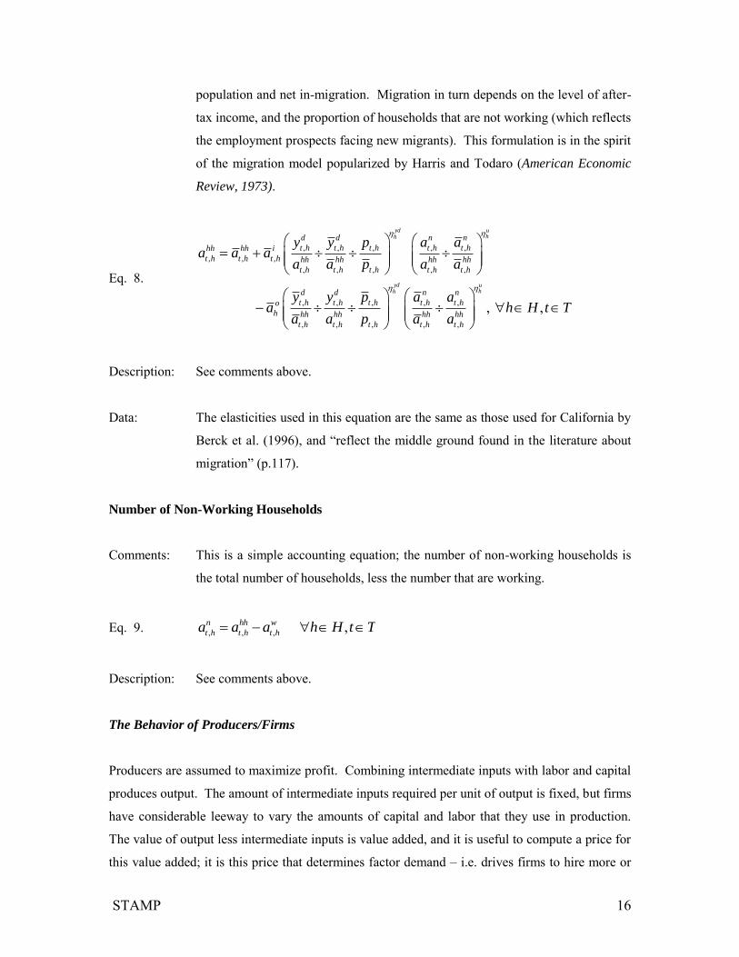
STAMP 16

population and net in-migration. Migration in turn depends on the level of after-

tax income, and the proportion of households that are not working (which reflects

the employment prospects facing new migrants). This formulation is in the spirit

of the migration model popularized by Harris and Todaro (American Economic

Review, 1973).

Eq. 8.

, , , , ,, , ,

, , , , ,

, , , , ,

, , , , ,

,

yd uhh

yd uhh

d d n n

t h t h t h t h t hhh hh i

t h t h t h hh hh hh hh

t h t h t h t h t h

d d n n

t h t h t h t h t ho

h hh hh hh hh

t h t h t h t h t h

y y p a aa a a

a a p a a

y y p a aa h

a a p a a

, H t T

Description: See comments above.

Data: The elasticities used in this equation are the same as those used for California by

Berck et al. (1996), and “reflect the middle ground found in the literature about

migration” (p.117).

Number of Non-Working Households

Comments: This is a simple accounting equation; the number of non-working households is

the total number of households, less the number that are working.

Eq. 9. , , , ,n hh w

t h t h t ha a a h H t T

Description: See comments above.

The Behavior of Producers/Firms

Producers are assumed to maximize profit. Combining intermediate inputs with labor and capital

produces output. The amount of intermediate inputs required per unit of output is fixed, but firms

have considerable leeway to vary the amounts of capital and labor that they use in production.

The value of output less intermediate inputs is value added, and it is useful to compute a price for

this value added; it is this price that determines factor demand – i.e. drives firms to hire more or

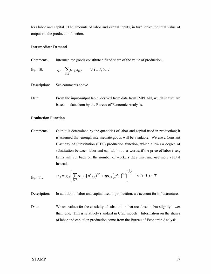
STAMP 17

less labor and capital. The amounts of labor and capital inputs, in turn, drive the total value of

output via the production function.

Intermediate Demand

Comments: Intermediate goods constitute a fixed share of the value of production.

Eq. 10. , , , , ,t i t i i t i

i I

v = q i I t T

Description: See comments above.

Data: From the input-output table, derived from data from IMPLAN, which in turn are

based on data from by the Bureau of Economic Analysis.

Production Function

Comments: Output is determined by the quantities of labor and capital used in production; it

is assumed that enough intermediate goods will be available. We use a Constant

Elasticity of Substitution (CES) production function, which allows a degree of

substitution between labor and capital; in other words, if the price of labor rises,

firms will cut back on the number of workers they hire, and use more capital

instead.

Eq. 11. -1

, , , , , , , ,i

i id

t i t i t f i t f i t i t

f F

q u g gk i I t T

Description: In addition to labor and capital used in production, we account for infrastructure.

Data: We use values for the elasticity of substitution that are close to, but slightly lower

than, one. This is relatively standard in CGE models. Information on the shares

of labor and capital in production come from the Bureau of Economic Analysis.

STAMP 18

Price of Value Added

Comments: Define value-added as the value of output less the cost of intermediate inputs.

One may then define a “price” of value added, which we then use below in the

factor demand (i.e. labor demand, capital demand) equations.

Eq. 12. , , , , , , ,1 ,va d v

t i t i t i i t i t g i

i I g GS

p p p i I t T

Description: Price of value-added by industry is the domestic price by industry minus the

production prices by industry according to their share in domestic supply,

including taxes on intermediates, if any.

Data: Prices are set equal to unit in the baseline case.

Factor Demand

Comments: It is possible to construct a profit function that expresses profits as a function of

factor inputs. Microeconomic theory shows that the partial first derivative of the

profit function, with respect to a given factor demand variable, gives the demand

equation for that factor. The left hand side of the equation shows payments to

labor (including the cost of factor taxes such as the employer share of social

security contributions). The right hand side gives the amount of value added

attributable to the factor. There are separate equations for labor and for capital,

for each of the 27 industrial sectors.

Eq. 13. , , , , , , , , , , , ,1 ,a x d va

t f i t f t f g i t f i t i t i t f i

g GF

r r + u p q i I, f F t T

Description: The factor demand at the current intra-industry rental rate (for labor and capital)

times the overall rental rate, including factor taxes is a function of the price of

value-added times the industry domestic supply.

Data: Information on the wage bills comes from the Bureau of Economic Analysis.

The total wage bill is divided by the number of workers (from the Bureau of

STAMP 19

Labor Statistics) to get measures of wage rates by industry. The intersectoral

wage differentials are not allowed to vary within the model. The cost of capital

was derived as property-type income divided by the capital stock. The capital

stock was constructed by disaggregating the national aggregate level of capital

using a series of proxy measures; further details of the methodology are provided

in Appendix 2 of the Texas State Tax Analysis Modeling Program: Texas-

STAMP (1999) and although this refers to Texas, the same approach was taken in

computing the capital stock for .

Factor Income

Comments: The total income accruing to factors – i.e. to labor and capital – is computed here.

Eq. 14. , , , , , , , , , , , ,a d a d

t f t f i t f t f i t f g t f t f g

i I g G

y r r u r r u f F t T

Description: The factor income is the sum of factor demand times rental rates, for all

industries and government sectors.

Trade with other States and Countries

From a state perspective, the “rest of the world” consists of the remainder of the United States as

well as the world outside the U.S. Goods produced in the sate are assumed to be close, but not

perfect, substitutes for goods produced elsewhere. Thus if prices rise in the state, the state’s

exports will fall and its imports will rise, but the adjustment need not be very large. There is no

need for trade to be balanced; capital flows simply adjust to cover the gap between exports and

imports. In this section we also develop a measure of the average price faced by domestic

households and firms for goods and services produced by each industry, the price is a weighted

average of the price of locally produced and imported goods.

Demand for Exports

Comments: Exports depend on the price of goods within the sate relative to the price outside

the state. If the domestic price rises relative to the foreign price, exports will fall.

Note that the elasticity here is negative.

STAMP 20

Eq. 15. , ,, ,

, ,

,1

ei

d w

t i t i

t i t i m

t g i

g G

p pe e i I t T

Description: Current exports are a function of baseline exports adjusted by the change in

domestic prices versus fixed world prices.

Data: The trade data for the state are not particularly reliable; we have used our

judgement, combined with BEA data, to arrive at sensible estimates. The

elasticities we use are similar to those employed by Berck et al.

Domestic Share of Domestic Consumption

Comments: The demand for imports is handled indirectly, by modeling the share of domestic

consumption that is supplied by domestic firms (d), following the approach

pioneered by Armington (1969). This share depends on the domestic price

relative to the price of the same goods in the rest of the world. We ignore import

tariffs on the grounds that they are a tiny fraction (less than 1%) of the value of

goods imported into the state.

Eq. 16. , ,, ,

, ,

,1

di

d w

t i t i

t i t i m

t g i

g G

p pd d i I t T

Description: See comments above.

Data: As with export demand we have used our judgement, combined with BEA data,

to arrive at sensible estimates. Intermediate Demand for Imports

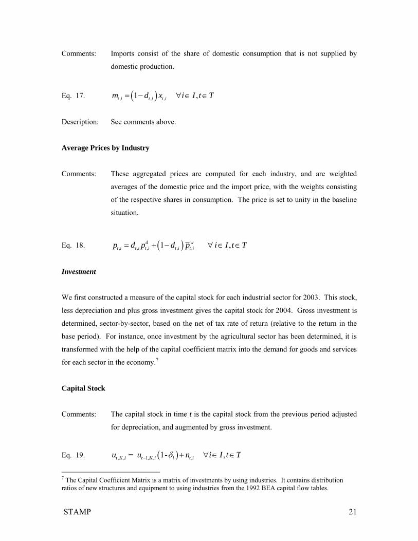
STAMP 21

Comments: Imports consist of the share of domestic consumption that is not supplied by

domestic production.

Eq. 17. , , ,1 ,t i t i t im d x i I t T

Description: See comments above.

Average Prices by Industry

Comments: These aggregated prices are computed for each industry, and are weighted

averages of the domestic price and the import price, with the weights consisting

of the respective shares in consumption. The price is set to unity in the baseline

situation.

Eq. 18. , , , , ,1 ,d w

t i t i t i t i t ip d p d p i I t T

Investment

We first constructed a measure of the capital stock for each industrial sector for 2003. This stock,

less depreciation and plus gross investment gives the capital stock for 2004. Gross investment is

determined, sector-by-sector, based on the net of tax rate of return (relative to the return in the

base period). For instance, once investment by the agricultural sector has been determined, it is

transformed with the help of the capital coefficient matrix into the demand for goods and services

for each sector in the economy.7

Capital Stock

Comments: The capital stock in time t is the capital stock from the previous period adjusted

for depreciation, and augmented by gross investment.

Eq. 19. , , 1, , , 1- ,t K i t K i i t iu u n i I t T

7 The Capital Coefficient Matrix is a matrix of investments by using industries. It contains distribution ratios of new structures and equipment to using industries from the 1992 BEA capital flow tables.

STAMP 22

Description: See comments above.

Data: A complete discussion of the construction of capital stock figures is given in

Texas State Tax Modeling Program: Texas-STAMP (1999); the same approach

and the same data sources are used for the state.

Gross Investment by Sector of Destination

Comments: The amount of gross investment in any given sector depends on the after-tax rate

of return in that sector relative to the return in the base period. The terminology

here can be confusing; investment destined for agriculture, for instance, consists

of the purchases of goods that will add to the capital stock in the agricultural

sector; the goods themselves will mainly come from other sectors (the sectors of

source).

Eq. 20. , , , , , , ,

, ,

, , , , , , ,

1 ,

1

i

x

t K i t g K i t K i

g GK

t i t i

t K i t g K i t K i

g GK

r u

n n i I t T

r u

Description: Gross investment is the baseline gross investment by industry adjusted to the

change in after-tax capital rental rates.

Data: The rate of return is computed as the property-type income for each sector (from

BEA) divided by the capital stock (authors’ computations). Based on the

econometric results from STAMP models estimated for the state and elsewhere,

we estimated the investment demand elasticity to be about 0.3.

Gross Investment by Sector of Source

Comments: Given that investment has been determined for each sector of destination, this

equation allows one to determine who will actually produce the investment

goods. This is done with the help of a capital coefficient matrix.

STAMP 23

Eq. 21. , , , , , ' , ''

1 ,n

t i t g i t i i i t i

g GS i I

p cn n i I t T

Description: The gross investment by source in after-tax prices is a function of investment by

destination according to the capital coefficient matrix.

Data: Based on the 1992 capital coefficient matrix for the United States from the

BEA/Department of Commerce.

Government

Government derives income from a wide range of taxes. It purchases goods and services and

makes transfers (such as pensions) to individuals. Some government spending is assumed to

remain unchanged even if tax revenues vary; the rest of spending is endogenous, in that it

responds to the availability of funds. Notionally, most revenues flow into the state General Fund;

they are then used in part to buy goods and services, but some are also transferred to local

government units.

Government Income

Comments: This equation adds up government income from multiple sources, including

indirect taxes (sales, motor fuels) and direct taxes (income, franchise tax).

Eq. 22.

0, , , , , , , , , , , , , , , , , , , , , , , ,

, , , , , , , , , , , , , , , ,

v m c n g

t g t g i t i t i t g i t i t i t g i t i h t i t g i t i n t i t g i t i g t i

i I i I h H i I i I i I g G

x a d x a d

t g f i t f i t f t f i t g f g t f g t f t f g

i I f F g G f F

y v p m pw c p cn p c p

r r u r r u

, , , , , , , ,

,

fh pi hh h hh

t g f t f t h g t h t h g h

f F h H h H

y a a

g G t T

Description: Income by government sector is the sum of taxes on intermediates, imports,

consumption, investment, government consumption, factors, income taxes and

other household taxes.

STAMP 24

Government Endogenous Purchases of Goods and Services

Comments: Spending on these items is assumed to take a fixed fraction of total government

receipts (from taxes and net intergovernmental transfers, less government

savings). The endogenous sectors are state spending on education, health, safety,

transport and “other,” and local spending on education and health.

Eq. 23.

, , , , , , , , , , , , , , , , , , ,1

, ,

g n pc

t i t g i t i g i g t g t g g t g g t ussstx g t h g t h t h g t g

g GS g G g G h H

p cg y b b b w a s

i I g GN t T

Description: The government spending in after-tax prices computed according to their share of

government income plus net inter-government transfers less government savings

and transfer payments. Note that only state and local governments are

endogenous in the model.

Data: The shares of spending going to these sectors are based on a careful analysis of

the state government budget and financial reports.

Government Endogenous Rental of Factors

Comments: As in the case of goods and services, government is also assumed to devote a

fixed share of its total spending to the purchase of labor and capital services for

those sectors considered to be endogenous.

STAMP 25

Eq. 24.

, , , , , , , , , , , , , , , , , , , , ,d a n pc

t f g t f t f g f g t g t g g t g g t ussstx g t h g t h t h g t g

g G g G h H

u r r y b b b w a s f F g GN t T

Description: The government factor demand is computed according to the share of each

government in total government spending, including net inter-government

transfers, less savings and transfer payments.

Government Infrastructure Capital Stock

Comments: The government adds to its infrastructure capital stock through its spending on

the government transportation sector, STTRAN.

Eq. 25.

Tt

bbbgkgkGg

gLOTRANt

Gg

STTRANgt

Gg

gSTTRANttt

,,1,,1,,11 1

Description: The infrastructure capital stock for the current year is the infrastructure for the

previous year, less depreciation plus the net spending on transportation by state

and local governments.

Data: The data for government infrastructure capital stock is based on national data

from the BEA.

Government Savings

Comments: Government saving is a residual, consisting of revenue less spending.

Eq. 26. , , , , , , , , , , , , , , ,

, , , , ', , , , , '' '

1 1

+ ,

g d a x

t g t g t i g t i t g i t f g t f g t f t f g g

i I g GS f F g GF

n pc

t h g t h hg t g g t ussstx g t g g

h H g G g G

s y cg p u r r

w a b b b g G t T

STAMP 26

Description: Government savings is the residual from government income, after spending and

factor rental, transfer payments, plus net inter-governmental transfers.

Distribution of Taxes to Spending and Transfers

Comments: Tax units, in this case those sectors collecting state revenues, distribute some of

their receipts to spending units, and others directly in the form of transfers to

households. The matrix IGTD (in the miscellaneous input file) identifies which

units pass on their revenues to other spending units, and the flows are recorded in

this equation.

Eq. 27. , , , , , , , , , , , ,n pc

t g g t g g t g t h g t h t h g t g

h H

b y w a s g g G

Description: The intra-fund accounting to distribute the government income, less transfer

payments and savings.

Data: This equation is based on institutional arrangements in place in the state.

Endogenous Distribution of Funds

Comments: This equation details the flows from state funds to state spending sectors and

from state spending sectors to local spending sectors.

Eq. 28.

Ggg

wwbb ROWSCTgINVESTg

g

ggtggtggt

',

,','''

'',',',,',,

Description: Some funds are fixed to the original share.

Data: Based on an analysis of the current pattern of spending in the state.

STAMP 27

State Personal Income

Comments: This equation defines state personal income as earnings (from labor and capital)

plus transfer payments.

Eq.29.

Hh Gg

pc

gh

n

htght

Hh

ht

s

t Ttawyy ,,,,,

Description: State personal income is the sum of household income and government transfer

payments.

Model Closure

Labor Market Clearing

Comments: Labor supply equals labor demand. For this to occur, the wage rate must adjust

to bring about this market clearing.

Eq. 30. Ttua t

Zz

d

zLt

Hh

w

ht

,,,

Description: Total working households equals the sum of private employment and government

employment.

Capital Market Clearing

Comments: Capital markets also clear for each sector. In other words, demand for capital by

industries equals supply of capital.

Eq. 31. , , , , ,s d

t K i t K iu u i I t T

Description: See comments above.

STAMP 28

Goods Market Clearing

Comments: Domestic demand (intermediate, consumer, government and investment demand)

plus exports less imports must equal domestic supply.

Eq. 32. t,i t,i t,i t,iq x e -m i I ,t T

Description: See comments above.

Domestic Demand Defined

Comments: These equations define domestic demand for each sector.

Eq.33. , , , , , , , ,t i t i t i h t i g t i

h H g G

x v c cg cn i I t T

Description: Domestic demand is the sum of intermediate demand, household consumption,

government consumption and investments.

PIT for Non Income Tax Units

Comments: This equation sets the personal income tax for non-income tax units to zero; this

is a technicality that ensures the solution to the model does not create income tax

revenue in an inappropriate place.

Eq.34. , , 0 ,t g ht h H,g GI t T

Set Intergovernmental Transfers to Zero if Not in Original SAM

Comments: This is another housekeeping equation that ensures the solution to the model does

not create inter-governmental transfers where they should not occur.

Eq.35. , , 0 , , where 0t g g ggb g g G t T b

STAMP 29

Federal Social Security Transfers to

Comments: Transfers paid to households from the Federal social security system are assumed

to be mainly determined by the number of households in the state.

Eq.36. ,t,h,USSSTX t,h,USSSTX

,

n

t h

t h

ab b

a

Description: Transfer payments are adjusted by the change in nonworking households.

Fix Exogenous Federal Transfers to Households

Comments: Federal transfers to households are assumed to vary with the number of

households in the state.

Eq.37. ,t,h,USNOND t,h,USNOND

,

n

t h

n

t h

ab b

a

Description: Transfer payments are adjusted by the change in nonworking households.

Fix Goods and Services Demand by Exogenous Government Units

Comments: The purchases of goods and services by some government sectors are considered

to be exogenous to the model. This equation fixes these values.

Eq. 38. , , , , ,t i g t i gcg cg i I,g GX t T

Fix Factor Rentals Paid by Exogenous Government Units

Comments: The purchases of the services of labor and capital are considered to be exogenous

to the model. This equation fixes these values.

Eq. 39. , , , , ,d d

t f g t f gu u f F,g GX t T

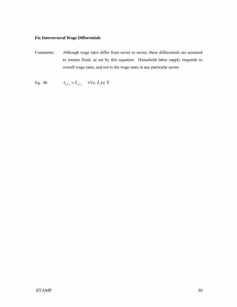
STAMP 30

Fix Intersectoral Wage Differentials

Comments: Although wage rates differ from sector to sector, these differentials are assumed

to remain fixed, as set by this equation. Household labor supply responds to

overall wage rates, and not to the wage rates in any particular sector.

Eq. 40. , , , , ,t L i t L ir r i I t T

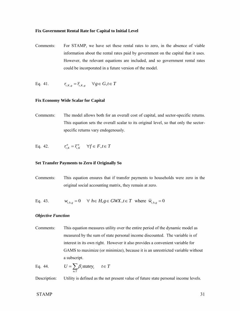
STAMP 31

Fix Government Rental Rate for Capital to Initial Level

Comments: For STAMP, we have set these rental rates to zero, in the absence of viable

information about the rental rates paid by government on the capital that it uses.

However, the relevant equations are included, and so government rental rates

could be incorporated in a future version of the model.

Eq. 41. , , , , ,t K g t K gr r g G t T

Fix Economy Wide Scalar for Capital

Comments: The model allows both for an overall cost of capital, and sector-specific returns.

This equation sets the overall scalar to its original level, so that only the sector-

specific returns vary endogenously.

Eq. 42. , , ,a a

t K t Kr r f F t T

Set Transfer Payments to Zero if Originally So

Comments: This equation ensures that if transfer payments to households were zero in the

original social accounting matrix, they remain at zero.

Eq. 43. , , , ,0 , where 0t h g t h gw h H,g GWX t T w

Objective Function

Comments: This equation measures utility over the entire period of the dynamic model as

measured by the sum of state personal income discounted. The variable is of

interest in its own right. However it also provides a convenient variable for

GAMS to maximize (or minimize), because it is an unrestricted variable without

a subscript.

Eq. 44. t t

t T

U statey t T

Description: Utility is defined as the net present value of future state personal income levels.

STAMP 32

Elasticity Assumptions for STAMP

For the model to work, one has to introduce values for the relevant elasticities. These are drawn

from the existing literature, as follows:

ETAM: Import elasticity with respect to domestic price for producers’ purchase of intermediates.

Most of the data on elasticities are taken from Reinert, Roland-Holst, and Shiells. The two most

recent are Reinert and Roland-Holst (1992)8 and Roland-Holst, Reinert and Shiells (1994)9.

In the first study, the authors estimate an Armington model for 163 mining and manufacturing

sectors. Two-thirds of the elasticities were positive and statistically significant, ranging from a

low of 0.13 for chocolate to 3.49 for wine, brandy and brandy spirits. The second study looked at

the impact of NAFTA. In this study many of the aggregate industries had an elasticity of 1.50.

Since import data for goods between states is almost impossible to obtain, we made some

assumptions and used 1.50 for most industries and a slightly lower elasticity of 0.50 for a handful

of less traded industries such as service industries.

While these elasticities are slightly higher than the literature on national trade, we believe that

goods in a state are more price-sensitive to goods in the Rest of the World (including other states)

than national goods. Therefore, we converted the elasticities to a domestic share elasticity for

each industry using the following equation. ETAD = ETAM * IMPORT / (DOM. DEMAND *

DOM. SUPPLY SHARE OF DOM. DEMAND). The estimates for this elasticity were taken

from the literature.

ETAE: Export elasticity with respect to domestic price for the sale producers’ goods. Used in the

export demand equation. The NAFTA study was also helpful with exports. We used an elasticity

of 1.65 for industries which had an import elasticity of 1.50 and an export elasticity of 0.65 for

those which had an import elasticity of 0.50.

SIGMA: Elasticity of substitution between capital and labor. Values in the literature range

between 0.15 and 1.809 for industries with the majority close to 1, and we have used values of 8K.A. Reinert and D.W. Roland-Holst. “Armington Elasticities for United States Manufacturing Sectors”. Journal of Policy Modeling. 14, no.5 (1992): 631-639. 9 D.W. Roland-Holst K.A. Reinert, and C.R. Shiells. “A General Equilibrium Analysis of North American Economic Integration”. Modeling Trade Policy: Applied General Equilibrium Assessments of North

American Free Trade. Cambridge Univ. Press (1994): 47-82.

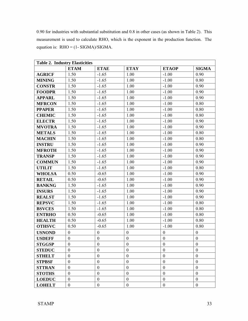
STAMP 33

0.90 for industries with substantial substitution and 0.8 in other cases (as shown in Table 2). This

measurement is used to calculate RHO, which is the exponent in the production function. The

equation is: RHO = (1- SIGMA)/SIGMA.

Table 2. Industry Elasticities

ETAM ETAE ETAY ETAOP SIGMA

AGRICF 1.50 -1.65 1.00 -1.00 0.90 MINING 1.50 -1.65 1.00 -1.00 0.80 CONSTR 1.50 -1.65 1.00 -1.00 0.90 FOODPR 1.50 -1.65 1.00 -1.00 0.90 APPARL 1.50 -1.65 1.00 -1.00 0.90 MFRCON 1.50 -1.65 1.00 -1.00 0.80 PPAPER 1.50 -1.65 1.00 -1.00 0.80 CHEMIC 1.50 -1.65 1.00 -1.00 0.80 ELECTR 1.50 -1.65 1.00 -1.00 0.90 MVOTRA 1.50 -1.65 1.00 -1.00 0.90 METALS 1.50 -1.65 1.00 -1.00 0.80 MACHIN 1.50 -1.65 1.00 -1.00 0.80 INSTRU 1.50 -1.65 1.00 -1.00 0.90 MFROTH 1.50 -1.65 1.00 -1.00 0.90 TRANSP 1.50 -1.65 1.00 -1.00 0.90 COMMUN 1.50 -1.65 1.00 -1.00 0.90 UTILIT 1.50 -1.65 1.00 -1.00 0.80 WHOLSA 0.50 -0.65 1.00 -1.00 0.90 RETAIL 0.50 -0.65 1.00 -1.00 0.90 BANKNG 1.50 -1.65 1.00 -1.00 0.90 INSURS 1.50 -1.65 1.00 -1.00 0.90 REALST 1.50 -1.65 1.00 -1.00 0.90 REPSVC 1.50 -1.65 1.00 -1.00 0.80 BSVCES 1.50 -1.65 1.00 -1.00 0.80 ENTRHO 0.50 -0.65 1.00 -1.00 0.80 HEALTH 0.50 -0.65 1.00 -1.00 0.80 OTHSVC 0.50 -0.65 1.00 -1.00 0.80 USNOND 0 0 0 0 0 USDEFF 0 0 0 0 0 STGGSP 0 0 0 0 0 STEDUC 0 0 0 0 0 STHELT 0 0 0 0 0 STPBSF 0 0 0 0 0 STTRAN 0 0 0 0 0 STOTHS 0 0 0 0 0 LOEDUC 0 0 0 0 0 LOHELT 0 0 0 0 0

STAMP 34

LOPBSF 0 0 0 0 0 LOTRAN 0 0 0 0 0 LOOTHS 0 0 0 0 0

The following elasticities are used in household-specific equations:

ETAPIT: Labor supply elasticity with respect to income taxes. This elasticity appears as an

exponent in the labor supply equation. Measurements were based on estimates taken from the

literature. The labor supply elasticities (ETARA) are widely divergent in the literature and suffer

from a lack of disaggregation. They range from close to zero to 2.3 for net wages, with rather

high positive values for women, particularly married woman. This means that the tax elasticities

are negative. There is some evidence of greater (absolute) tax elasticities at higher income levels,

which is why we assume a graduated scale from -0.15 for the lowest income category to -0.35 in

the top category (see Table 3).10

ETATP: Household response to transfer payments. The transfer payment elasticities reflect a

study by Robins (1985) on the effects of a negative income tax (NIT). It is also a reflection of the

observation that income received by upper income groups is on average largely unaffected by

transfer payments.

ETAYD: Responsiveness of immigration to after tax income. Not much literature exists that ties

migration to disposable income or unemployment. Studies by Bartik (1991), Valiant (1994), and

Treyz et al. (1993) put the range of responses to a change in wage rates at between 0.835 and

2.39. We used these as a basis for our after tax earnings elasticities. This elasticity appears in the

population equation.

ETAU: Responsiveness of immigration to unemployment. We made some assumptions based on

the responsiveness to employment elasticities in the literature.

ETAMH: Income elasticity of demand for imports by household. This elasticity appears in the

household import equation.

10 Note that ETAPIT = -ETARA (t/(1-t)), where t is the income tax rate.

STAMP 35

Table 3. Household-Related Elasticities

ETAPIT ETATP ETARA ETAYD ETAU ETAMH

LESS10 -0.15 -0.05 0.17 1.30 -0.80 0.70 LESS25 -0.18 -0.05 0.17 1.50 -0.80 0.70 LESS50 -0.20 -0.04 0.20 1.60 -0.80 0.70 LESS75 -0.25 -0.04 0.30 1.80 -0.80 0.70 LES100 -0.25 -0.03 0.40 2.00 -0.80 0.70 LES150 -0.30 -0.03 0.50 2.10 -0.80 0.70 MOR150 -0.35 -0.02 0.50 2.30 -0.80 0.70

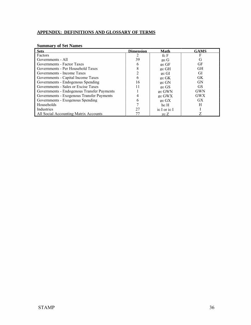
STAMP 36

APPENDIX: DEFINITIONS AND GLOSSARY OF TERMS

Summary of Set Names

Sets Dimension Math GAMS Factors 2 fF F Governments - All 39 gG G Governments - Factor Taxes 6 gGF GF Governments - Per Household Taxes 8 gGH GH Governments - Income Taxes 2 gGI GI Governments - Capital Income Taxes 6 gGK GK Governments - Endogenous Spending 16 gGN GN Governments - Sales or Excise Taxes 11 gGS GS Governments - Endogenous Transfer Payments 1 gGWN GWN Governments - Exogenous Transfer Payments 4 gGWX GWX Governments - Exogenous Spending 6 gGX GX Households 7 hH H Industries 27 iI or jI I All Social Accounting Matrix Accounts 77 zZ Z

STAMP 37

Summary of Parameter Names

Parameters Dimension Math GAMS Input Output Coefficients 77 x 77 - A(Z,Z1) Domestic Input Output Coefficients 27 x 27

ij AD(Z,Z1)

Government Spending Shares of Net Income 39 x 39 ig ,fg AG(Z,G) Factor Share Exponents in Production Function 2 x 27

fi ALPHA(F,I)

Initial Shares of Consumption 27 x 7 ih ALPHA(I,H) Deductibility of Taxes 3 x 3 gg

t ATAX(G,G1) Income Elasticities of Demand 27 x 7 ih BETA(I,H) Capital Coefficient Matrix 27 x 27 ij CCM(I,J) Depreciation Rate 27 i DEPR(I) Export Price Elasticities 27 i

e ETAE(I) Domestic Demand Elasticity 27 i

d ETAD(I) Investment Supply Elasticity 1 i ETAI L Supply Elasticity with respect to Average Wage 7 h

ls ETARA(H) Labor Supply Elasticity with respect to TP's11

7 htp ETATP(H)

Labor Supply Elasticity with respect to Taxes

7 hPIT ETAPIT(H)

Responsiveness of In-Migration to Unemployment 7 hu ETAU(H)

Responsiveness of In-Migration to Disp. Income 7 hyd ETAYD(H)

Production Function Scale 27 i GAMMA(I) Types of Inter-Government Transfers 39 x 39 - IGTD(G,G1) Correction Factor between Households and Jobs 1 JOBCOR Price Elasticities of Demand 27 x 27 ii’ LAMBDA(I,J) Miscellaneous Industry Parameters 27 x 10 - MISC(Z,*) Income Tax Table Data in Input File 7 x 8 - MISCG(G,H,*) Miscellaneous Household Parameters 7 x 8 - MISCH(H,*) Natural Rate of Population Growth 7 h NRPG(H) Substitution Exponent in Production Function 27

i RHO(I)

Social Accounting Matrix 77 x 77 zz’ SAM(Z,Z1) Consumption Sales and Excise Tax Rates 9 x 27 gi

c TAUC(G,I) Factor Tax Rates 5 x 2 x 77 gfz TAUF(G,F,Z)

Factor Taxes applied to Factors 5 x 2 - TAUFF(GF,G) Employee Portion of Factor Taxes 5 x 2 gf TAUFH(G,F) Experimental Factor Tax Rates 5 x 2 x 77 gfz

x TAUFX(G,F,Z) Government Sales and Excise Tax Rates 9 x 27 gi

g TAUG(G,I) Household Taxes other than PIT 1 x 7 gh TAUH(G,H)

Investment Sales and Excise Tax Rates 9 x 27 gin TAUN(G,I)

Sales and Excise Tax Rates 9 x 27 qiq TAUQ(G,I)

Intermediate Good Sales and Excise Tax Rates 9 x 27 giv TAUV(G,I)

Tax Bracket Base Amount 2 x 7 ghb TAXBASE(G,H)

Tax Bracket Minimum Taxable Earnings 2 x 7 ghd TAXBM(G,H)

Tax Constant to Correct Calculated to Observed 2 x 7 ghc TAXCVC(G,H)

Tax Deduction other than Standard and other PIT 2 x 7 gho TAXOD(G,H)

Percentage Itemizing 2 x 7 ghi TAXPI(G,H)

Tax Destination Shares 39 x 39 gg' TAXS(G,G1) Tax Deduction for Standard Deductions 2 x 7 gh

s TAXSD(G,H) Percent of Households Receiving TP’s 7 x 6 hg

pc TPC(H,G)

11 TP is abbreviation for transfer payments.

STAMP 38

Summary of Variable Names

Variables Dimension Math GAMS Public Consumption 27 x 39 cig CG(I,G) Private Consumption 27 x 7 cih CH(I,H) Gross Investment by Sector of Source 27 cin CN(I) Consumer Price Index 7 ph CPI(H) Exports 27 ei CX(I) Domestic Share of Domestic Consumption 27 di D(I) Domestic Demand 27 xi DD(I) Domestic Supply 27 qi DS(I) Sectoral Factor Demand 2 x 77 ufi

d, ufgd FD(F,Z)

Number of Households 7 ah HH(H) Number of Non-Working Households 7 ah

n HN(H) Number of Working Households 7 ah

w HW(H) Household Out-Migration 7 ah

o MO(H) Household In-Migration 7 ah

i MI(H) Inter-Governmental Transfers 37 x 37 Bgg’ IGT(G,G1) Capital Stock 27 uKi

s KS(I) Imports 27 mi M(I) Gross Investment by Sector of Destination 27 ni N(I) Net Capital Inflow 1 z NKI Aggregate Price 27 pi P(I) Aggregate Price including Sales/Excise Taxes 27 pi

c PC(I) Domestic Producer Price 27 pid PD(I)

Per Household Personal Income Taxes 2 x 7 tgh PIT(G,H) Producer Price Index 1 p PPI Value Added Price 27 pi

va PVA(I) World Price (Rest of US and Rest of World) 27 pi

w PW(I) Sectoral Factor Rental Rates 2 x 27 rfi, rfg R(F,I) Economy Wide Scalar for Factor Rental Rates 2 rf

a RA(F) Government Savings 39 sg S(G) Private Savings 7 sh S(H) State Personal Income 1 q SPI Transfer Payments 7 x 39 whg TP(H,G) Intermediate Goods 27 vi V(I) Factor Income 2 yf Y(F) Government Income 39 yg Y(G) Household Income 7 yh Y(H) Household after Tax Income including TP’s 7 Yh

d YD(H)

STAMP 39

The Beacon Hill Institute STAMP Development Team

David G. Tuerck is Executive Director of the Beacon Hill Institute for Public Policy Research at Suffolk University where he also serves as Chairman and Professor of Economics. He holds a Ph.D. in economics from the University of Virginia and has written extensively on issues of taxation and public economics.

Paul Bachman is Director of Research at the Beacon Hill Institute for Public Policy Research at Suffolk University and a Senior Lecturer in Economics Suffolk University. He holds a Master of Science in International Economics from Suffolk University. Michael Head, MSEP is an Economist at the Beacon Hill Institute. He holds a Master of Science in Economic Policy from Suffolk University.