WORKSHOP ON STOCK ASSESSMENT METHODS - · PDF fileHow to model selectivity: functional form,...

INTER-AMERICAN TROPICAL TUNA COMMISSION

WORKSHOP ON STOCK ASSESSMENT METHODS La Jolla, California (USA)

7-11 November 2005

REPORT Compiled by Mark N. Maunder

TABLE OF CONTENTS 1. Introduction..................................................................................................................................... 1 2. Review of models: .......................................................................................................................... 1 2.1. A-SCALA ....................................................................................................................................... 1 2.2. MULTIFAN-CL ............................................................................................................................. 2 2.3. Stock Synthesis II ........................................................................................................................... 3 2.4. CASAL ........................................................................................................................................... 3 2.5. CCSBT operating model................................................................................................................. 3 3. Application of the models to yellowfin tuna data........................................................................... 4 4. Discussion of the models ................................................................................................................ 4 5. Questions: ....................................................................................................................................... 4 5.1. How to model fishing mortality: Pope’s approximation, effort deviates (MULTIFAN-CL),

solving the catch equation, or virtual population analysis (VPA)-type annual variation in selectivity ........................................................................................................................................ 4

5.2. How to model selectivity: functional form, smoothness penalties, cubic splines .......................... 5 5.3. Do we need to integrate across random effects (e.g. recruitment deviates) and estimate standard

deviations? ...................................................................................................................................... 5 5.4. How to estimate uncertainty: Bayesian; profile likelihood; bootstrap;model uncertainty ............. 6 5.5. How to include environmental data ................................................................................................ 6 5.6. How to perform forward projections .............................................................................................. 6 5.7. What likelihood functions to use for different data sets and how to weight data sets in the

assessment....................................................................................................................................... 7 5.8. Should we use spatial structure in the population dynamics, or are spatially-defined fisheries

adequate?......................................................................................................................................... 7 6. Other topics..................................................................................................................................... 8 6.1. Including prior information in stock assessment models................................................................ 8 6.2. Can general fisheries models be used for protected species modeling? ......................................... 8 6.3. Distributed computing .................................................................................................................... 8 7. Recommendations for solving the eight questions ......................................................................... 8 8. Recommendations for additions to the models............................................................................. 10 8.1. Changes that would be most easily incorporated by modification of the existing A-SCALA code

(Recommendation are listed in order of perceived importance.).................................................. 10 8.2. Changes that would likely require a move to another modeling platform or significant rewriting

of the A-SCALA code .................................................................................................................. 11 9. Recommended research ................................................................................................................ 11 10. References..................................................................................................................................... 12 11. Appendix A. Participants .............................................................................................................. 13 12. Appendix B. Comparison of the four models discussed at the workshop .................................... 14 13. Appendix C. Background information.......................................................................................... 17

Report - Assessment methods workshop, Nov 2005 1

1. INTRODUCTION

The IATTC holds an annual technical workshop on a topic that is of significant importance to the stock assessment of tunas and billfishes in the eastern Pacific Ocean (EPO). The topic of the workshop of November 2005 arose from research needs identified at the annual review of the sixth meeting of the IATTC Working Group on Stock Assessment, held in May 2005.

The workshop reviewed alternative stock assessment methods. In particular, A-SCALA, the current method used by the IATTC to assess tunas in the EPO , was compared to other general stock assessment models: 1) MULTIFAN-CL, used by the Secretariat of the Pacific Community (SPC) for tuna stock assessments in the western and central Pacific Ocean (WCPO) and for the Pacific-wide bigeye tuna assessment; 2) Stock Synthesis II, used to assess groundfish on the west coast of the United States; and 3) CASAL, used for stock assessments in New Zealand by the National Institute of Water and Atmospheric Research (NIWA). Other assessment methodologies were also discussed. The outcome of the workshop will influence the future direction of stock assessment methodology for assessing tunas in the EPO.

The specific questions that were addressed during the workshop were:

1) How to model fishing mortality: Pope’s approximation, effort deviates (MULTIFAN-CL), solving the catch equation, or virtual population analysis (VPA)-type annual variation in selectivity;

2) How to model selectivity: functional form, smoothness penalties, cubic splines;

3) Do we need to integrate across random effects (e.g. recruitment deviates) and estimate standard deviations?

4) How to estimate uncertainty: Bayesian; profile likelihood; bootstrap; model uncertainty;

5) How to include environmental data;

6) How to perform forward projections;

7) What likelihood functions to use for different data sets and how to weight data sets in the assessment;

8) Should we use spatial structure in the population dynamics, or are spatially-defined fisheries adequate?

This document summarizes the presentations made during the workshop, provides answers to the questions, makes recommendations on changes to the IATTC stock assessments and for future research. Information from discussions arising in the workshop is integrated into these sections.

During the workshop several tables (Appendix 2) were created describing the differences among the four models compared at the workshop.

In preparation for the workshop, a background document providing information on the assessment models and the questions to be considered at the workshop was sent to participants. This document was updated based on information from the workshop (Appendix 3) and it contains more technical details than the summaries presented below.

2. REVIEW OF MODELS:

2.1. A-SCALA

Mark Maunder gave an introduction to integrated stock assessment models and A-SCALA. Integrated analysis consists of including all available data into a single statistical analysis. For example, modern statistical stock assessment models generally include age or length-frequency data and indices of abundance from catch-per-unit-of-effort (CPUE) data or surveys. These analyses can be used to estimate management quantities such as maximum sustainable yield (MSY), provide forward projections, and


represent uncertainty in these estimates or projections.

A-SCALA (age-structured statistical catch-at-length analysis) is the stock assessment model developed by the IATTC staff to assess tunas in the EPO. It is based on the MULTIFAN-CL approach, described in subsection 2.2., and fits a population model to catch and length-frequency data conditioned on effort. It also allows the use of prior information to inform or constrain many of the parameter values.

Two main characteristics of A-SCALA are the inclusion of length-frequency data into the analysis and the method used to model fishing mortality. Rather than converting length-frequency data to age outside the model and then using the age-frequency data in the model, A-SCALA (and the other models compared in the workshop) fits models directly to the length-frequency data. This method ensures consistency throughout the analysis, and allows information from all the data sets to convert length-frequency into age and estimate growth parameters. It also makes sure that the proportions at age used to convert length-frequency into age are consistent with the assumed population dynamics.

A-SCALA uses the effort deviate approach to model fishing mortality. This method assumes that there is error in the observed catch data, and models fishing mortality proportional to effort with parameters estimated to represent temporal deviates in this relationship. The temporal deviates are penalized, based on a distributional assumption. A-SCALA also uses the separability assumption that separates fishing mortality into age (selectivity) and time components, with the age component constant over time. This differs from virtual population analysis (VPA) approaches, which allow age-specific fishing mortality to change freely with time.

More information on A-SCALA can be found in Maunder and Watters (2003) describing its initial development and in subsequent Stock Assessment Reports (e.g. Maunder and Hoyle 2006) which describe modifications.

2.2. MULTIFAN-CL

Pierre Kleiber presented an overview of MULTIFAN-CL and the changes that have been made to it in the past year. MULTIFAN-CL (Fournier et al. 1998; Hampton and Fournier 2001) is a statistical, size-based, age-structured, and spatial-structured stock assessment model. It accommodates variable, region-specific recruitment, fleet-specific selectivity, and time-varying catchability. Fleet characteristics can be grouped, if desired, to reduce the number of estimated parameters. Input data consist of catch, effort, size samples, and tagging data if available. Sample data can be by length, by weight, or both. Strata with missing catch, or effort, or sample data are accommodated appropriately. Bayesian priors can be applied to many of the basic parameters and to various derived parameters. Model fitting proceeds in phases, and can be orchestrated by a "doitall" file that specifies properties and order of the phases.

Output from MULTIFAN-CL is voluminous, consisting of a variety of diagnostic results and stock assessment information. The latter includes various MSY-related reference points, such as the ratio of fishing mortality to fishing mortality that supports MSY (F/FMSY) and the ratio of biomass to biomass that supports MSY (B/BMSY). Also available are fishery impact results, which are estimates of abundance trajectories under hypothetical regimes of reduced, or eliminated, fishing effort. Statistical uncertainty is estimated using the inverse Hessian matrix and from likelihood profiles that can be generated by forcing model fits to a range of target values for a parameter of interest.

MULTIFAN-CL is accompanied by various utilities to aid in constructing input files and visualizing and interpreting output files. These include two function packages for the statistical and graphics program, R. A user guide for MULTIFAN-CL is available.

Several developments and improvements to MULTIFAN-CL occurred in the past year. Selectivity can now be specified by cubic spline curves, which reduces the number of parameters to estimate. The system for projecting biomass estimates into the future has been improved. Seasonality and regional variation in recruitment have been included in the process of estimating the age distribution at the start of


the time series. More flexibility in specifying recruitment seasonality has been incorporated, as well as output to facilitate likelihood profiling. Improvements and updates are continually made to the R graphics and other utilities and also to the User Guide. More information on MULTIFAN-CL and updated documentation can be found at http://www.multifan-cl.org/.

2.3. Stock Synthesis II

Richard Methot presented an overview of Stock Synthesis II (SS2). SS2 is a general stock assessment model developed to assess groundfish off the west coast of the USA. It is the second generation version of the original Stock Synthesis developed in 1988. It is programmed using AD Model Builder, thus inherits all ADMB features and functions. It has several modifications over the previous version of Stock Synthesis, including better variance estimation through ADMB features, Pope’s (1972) approximation (i.e. removing catch instantaneously halfway through the year) to model fishing mortality, growth morphs to approximate size-based survival, and meta-population structure to address spatial issues.

SS2 can accept a variety of data types: catch, survey abundance, fishery CPUE, age and/or size composition (including age at size composition), discard, and mean body weight. SS2 includes several age and/or size-selectivity parameterizations, including a general functional form represented by the double logistic. Ageing imprecision is incorporated in the analysis of age composition data. Each sex can be modeled as a collection of growth morphs, which allows size-specific selectivity to modify the overall length-at-age distribution. SS2 has a general representation of model parameters that includes environmental variables, temporal deviates, time blocks, and offsets from other parameters. SS2 allows control of parameter estimation, including bounds, initial or fixed values, phase of estimation, and priors. SS2 contains estimation of relevant MSY-related management quantities, and can conduct forecasts that incorporate estimates of imprecision. An Excel file is available to view the results, some of which are output in a database format for ease of interrogation and presentation. A Graphics User Interface with context-sensitive help is being developed and will be available in early 2006 from the NMFS Stock Assessment Toolbox website http://nft.nefsc.noaa.gov/ with email to [email protected].

2.4. CASAL

Chris Francis presented an overview of CASAL, which was designed in 2001 as a general-purpose stock assessment program for use in New Zealand. A primary concern in its design was the desire to give analysts maximum flexibility in individual applications. To this end, the two concepts that are implicit in many assessment models–the population partition and the annual cycle–were formalised and included explicitly. CASAL allows a wide range of observation types, observation error structures, and prior distributions. A pseudo observation construct allows the user great flexibility in model outputs. In addition to point estimation and Monte Carlo Markov Chain (MCMC) Bayesian analysis, the model can automatically calculate profiles, projections, and various types of deterministic and stochastic yields. The program is written in C++ and uses automatic differentiation (based on the freeware ADOL-C) to make estimation more efficient. It may be downloaded from the web (file latest_casal.zip at ftp://ftp.niwa.co.nz/software/casal).

2.5. CCSBT operating model

Hiroyuki Kurota presented a summary of the southern bluefin tuna (SBT) operating model used for management procedure evaluation. This model includes many of the features of the other general models discussed at the workshop. It was designed to imitate the SBT dynamics and fishing processes with realistic uncertainty, to fit to historical data to estimate parameters like stock assessment models, and originated from a stock assessment model for SBT. The model includes standardized longline CPUE indices, catch-at-age data, catch-at-length data, and tagging data. One interesting feature of the model is that selectivity is allowed to vary over time. A Bayesian approach based on gridding the analysis over several assumptions and weighting each scenario based on either a priori weights or using the likelihood of the fit is used to represent uncertainty for management strategy evaluation.

http://www.multifan-cl.org/

http://nft.nefsc.noaa.gov/

mailto:[email protected]

ftp://ftp.niwa.co.nz/software/casal


3. APPLICATION OF THE MODELS TO YELLOWFIN TUNA DATA

Simon Hoyle presented results from fitting the different models to data for yellowfin tuna in the EPO. There were substantial difficulties in applying SS2 and CASAL to the yellowfin data sets. In these two models, the yellowfin application was too large and used virtual memory which greatly increased the running time. This is because the current A-SCALA model has a large number of fisheries (16) and the length data are entered into the model in 1-cm bins. SS2 allows for different-sized bins, and restructuring the bins allowed estimation within SS2. When the number of length bins was reduced to 103, the SS2 model ran to completion in about 40 minutes. Similar restructuring of the bin sizes in CASAL may make the yellowfin application practical for the CASAL environment.

The results from the MULTIFAN-CL application were quite different from those from A-SCALA, probably because of the different assumptions about effective sample size for the catch-at-length data sets between the two analyses. The preliminary SS2 results were also somewhat different, but the reasons for the differences were not determined. Further work is needed on both analyses to develop a more comprehensive comparison.

4. DISCUSSION OF THE MODELS

During the workshop several tables were created describing the differences between the four models compared at the workshop. These tables are presented in Appendix 2.

5. QUESTIONS:

5.1. How to model fishing mortality: Pope’s approximation, effort deviates (MULTIFAN-CL), solving the catch equation, or virtual population analysis (VPA)-type annual variation in selectivity

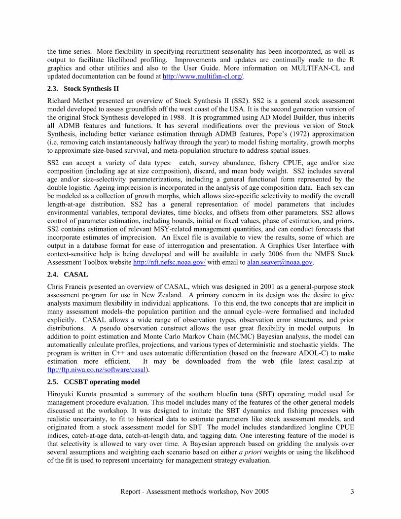
Richard Methot gave an introduction to the different methods that are used to model fishing mortality. A-SCALA and MULTIFAN-CL assume that there is error in the observed catch data, and make fishing mortality proportional to effort, with parameters estimated to represent temporal deviates in this relationship. The temporal deviates are penalized in accordance with a distributional assumption. SS2 and CASAL assume that catch is observed perfectly, and use Pope’s (1972) approximation to model the fishing mortality (catch is taken out halfway through the year).

There are two separate aspects of the parameterization of fishing mortality (F) in stock assessment models. One is the functional form of the mortality estimation. The two options are: 1) parameterize F as continuous throughout a time period (continuous F) and 2) parameterize F as an instantaneous removal at the middle of the time period (commonly termed Pope’s approximation–mid-period U). In reality, both are approximations of the actual time course of F and catch within a time period. The second issue is the way in which the level of mortality is estimated. Three options that have been used are: 1) each F is a free model parameter (free parameter); 2) F is updated continuously within the model to match the observed catch exactly (known catch); and 3) F is estimated as an offset from a general F-effort relationship (f(effort)).

Free parameter Known catch f(effort) Continuous F Ianelli models SS1;

CASAL (only one fishery) A-SCALA;

MFCL mid-period U SS2;

Coleraine CASAL (preferred)

The parameterization and estimation issues are not completely independent, and various factors may influence the best choice for a given situation. Some of these factors include:


BEST WORST Missing or imprecise catch

f(effort) Free parameter Known catch Missing or imprecise effort

Known catch Free parameter f(effort) Multiple fleets

Continuous F mid-period U High F

Continuous F mid-period U Smooth gradient

Continuous F – f(effort) Continuous F – free parameter mid-period U Speed

Mid-period U and known catch Continuous F and known catch, f(effort)

Free parameter

Parameter bloat Known catch f(effort) Free parameter

5.2. How to model selectivity: functional form, smoothness penalties, cubic splines

Pierre Kleiber presented an overview of how selectivity is modeled. Catchability can vary over both time and age. The separability assumption is often used to separate fishing mortality into age-specific (selectivity) and time-specific components. However, selectivity can also change over time. Estimating selectivity at each age (or size) class is parameter intensive, and can result in instability or lack of convergence. This can be overcome by constraints, imposing a mathematical form for selectivity, or interpolation within selectivities estimated at a reasonable number of ages (or sizes) (e.g. cubic spline interpolation).

Selectivity can be related to size, age, or both. As the models generally have an underlying age structure, the length-based selectivity is converted to an age equivalent. However, simply using the mean length-at-age to determine the selectivity does not fully account for the effect of length-based selectivity. To model the catch-at-length data correctly, the length-specific selectivity must be applied to the distribution of length at age.

5.3. Do we need to integrate across random effects (e.g. recruitment deviates) and estimate standard deviations?

Mark Maunder gave an introduction to the use of random effects in stock assessment models. Random effects can be used to model temporal changes in model parameters. They are used mainly for annual deviates in recruitment, but MULTIFAN-CL uses them for effort and catchability deviates. They could also be used for other processes such as selectivity, natural mortality, or growth. Most fisheries models use a penalized likelihood approach to model random effects, with the penalty based on the distributional assumption and the standard deviation of the penalty fixed. However, more traditional approaches integrate across the random effects and estimate the standard deviation of the random effects distribution.

Simulation tests of a model with recruitment as a random effect showed that integrating across the random effects provided better estimates of the standard deviation of the random effects distribution, particularly when catch-at-age data were not available for all years. The penalized likelihood method produces negatively biased estimates of the standard deviation. Good estimates of the standard deviation may be important for recruitment in projections and, in the case of A-SCALA and MULTIFAN-CL, for weighting catch and effort data.

Random effects can be applied in both a Bayesian and likelihood framework. Integrating across the random effects is more convenient in a Bayesian MCMC framework, but this requires priors for all model parameters. However, for both frameworks the analysis is very computationally intensive for complex


stock-assessment models, and is not practical for the current A-SCALA assessments. AD Model Builder now has Laplace approximation and importance sampling to do random effects modeling, with only a single line of modification to the code compared to penalized likelihood.

5.4. How to estimate uncertainty: Bayesian; profile likelihood; bootstrap;model uncertainty

Mark Maunder presented an introduction to estimating uncertainty. There are several methods that can be used to estimate uncertainty: normal approximation, profile likelihood, bootstrap, Bayesian integration, and sensitivity analysis; and several methods to present uncertainty: confidence intervals, confidence distributions, profile likelihoods, bootstrap distributions, credibility intervals, and posterior distributions. Traditionally hypotheses tests, confidence intervals, and sensitivity analyses have been used to represent or deal with uncertainty. More recently, likelihood and Bayesian approaches have become popular, and confidence distributions are being promoted. However, likelihood approaches are difficult to interpret, Bayesian analysis requires priors, and confidence distributions have the same interpretation as confidence intervals.

The different methods have different computational demands. Normal approximation requires only estimation of the Hessian matrix, Bayesian requires evaluation of the objective function millions of times, bootstrap requires optimization of the objective function hundreds of times, and profile likelihood requires optimization of the objective function tens of times for each quantity of interest.

Confidence distributions may be a way to unite Bayesian and frequentist frameworks, through the automatic calculation of objective posteriors. These objective posteriors have the desirable characteristics of good coverage and invariance to transformation. In this case the distributions for frequentist (confidence distribution) and Bayesian (posterior distribution) are the same, the uncertainty intervals (confidence interval and credibility interval) are the same, and the uncertainty intervals are usually interpreted in the same way (95% probability that the true value is in the interval).

5.5. How to include environmental data

Mark Maunder gave an introduction on how to include environmental data into stock assessment models. Environmental data can be included either as a structural component of the model or as a data series to which the model is fit. These approaches are identical in many situations, but may differ in accordance with the assumptions. Simulation analysis results suggest that the relationship should be integrated into the model, and when using a structural approach, additional process error should be modeled as a random effect. Integrating out the random effect may be appropriate.

In some cases the environmental data may not be available for all time periods. In this case the missing data may be estimated as a random effect, possibly with the parameters of the random effect distribution based on the mean and variance of the environmental data. Under the assumptions of normality for both the environmental index and the additional process error, it may be necessary only to modify the standard deviation of the process error random effect distributional assumption to account for missing environmental data.

5.6. How to perform forward projections

Mark Maunder gave an introduction to performing forward projections, using stock assessment models. There are several types of uncertainty that should be incorporated into forward projections: parameter, current status, model, and future demographic. The major sensitivity to this uncertainty depends on the length of the forward projection. Short-term projections are sensitive to uncertainty in current status and recent recruitments. Long-term projections are sensitive to uncertainty due to stochastic variation, structural assumptions (e.g. stock-recruitment relationship), and parameter uncertainty. Several methods have been used to carry out forward projections: stochastic projections from point estimates, sampling parameters from normal distributions and performing stochastic projections, likelihood methods that extend the estimation time frame to include the projection period, bootstrap, and Bayesian. The


computational demands differ among the methods: they are relatively low for point estimation methods and normal approximation to the likelihood method, and relatively high for the Bayesian, bootstrap, and profile likelihood methods. The normal approximation approach is used for the A-SCALA assessments because of the high computational demands of A-SCALA. However, the normal approximation approach must be modified due to bias caused by the ln(σ) term in the recruitment residual penalty and the lognormal bias correction term for future recruitment or effort deviates.

Projections require assumptions about the allocation of effort among the gears in the future. The estimates of age-specific fishing mortality rates in the most recent years are usually uncertain. Therefore, these estimates should not be used to represent future age-specific fishing mortality. However, because the fisheries change over time, historic estimates may not be good predictors of future age-specific fishing mortality. Therefore, a tradeoff must be made between recent and historic years to calculate age-specific fishing mortality for projections.

5.7. What likelihood functions to use for different data sets and how to weight data sets in the assessment

Chris Francis gave an introduction into the use of likelihood functions. Data weighting is of great importance in stock-assessment models, but it is a difficult problem, with no easy one-size-fits-all answer. The presentation described some techniques found of use in New Zealand stock assessments and concluded with a description of an unresolved problem. In general, it seems best to avoid subjective decisions and to express data weightings in terms of error parameters (e.g., coefficients of variation or sample sizes), rather than arbitrary parameters that are difficult to interpret. Where possible, it is useful to think of an error (difference between an observation and a model prediction) as being the sum of two terms: the observation error (difference between an observed value and the truth) and process error (difference between the truth and a model prediction). For many types of observations it is possible to quantify observation error (e.g., by bootstrapping the sampling process). Process errors can either be estimated by meta-analysis (e.g., Francis et al. 2003) or within the stock-assessment model.

The problem of correlation structure within length (and age) frequencies is unresolved. Such correlations may be substantial, but are traditionally not accounted for. This is most likely to cause problems in assessments where there are trends in mean length in length-frequency data. The error structures usually assumed for these data will tend to assign too much weight to these trends.

5.8. Should we use spatial structure in the population dynamics, or are spatially-defined fisheries adequate?

Adam Langley gave an introduction into the spatial structuring of stock assessment models. MULTIFAN-CL allows for the spatial structuring of both the population dynamics and the fisheries. MULTIFAN-CL also allows for the inclusion of tagging data that can provide information on the movement among regions. Assessments for the western and central Pacific Ocean (WCPO) typically have 4–6 regions for the population dynamics.

The population dynamics are structured spatially because the stock occupies a very large area, and processes may not be the same over the whole area. “Sub-populations” are identifiable within a stock area, the rates of mixing over the entire stock area are relatively low, there are different exploitation rates in different areas, recruitment processes are on a local scale, there are differences in biological parameters (e.g. growth) among areas, so modeling should incorporate investigation of “local”-scale management issues.

Regions should be defined on the basis of geographically-distinct areas, delineated by bio-oceanographic conditions, key fishery boundaries, relative abundance of species, management issues, availability of data to define abundance trend and size composition for regions (over time), homogeneity with respect to magnitude of CPUE and CPUE trends, and comparable size composition of catch. However, there is a trade-off between spatial resolution and data availability/model complexity.


The WCPO models generally have inadequate tagging data to determine movement among all regions. Therefore, to provide additional information about the relative size of the populations in each region, the catchability for the longline fisheries is shared among regions so the catch rates provide information on the relative abundance. Unfortunately, for some populations the estimated movements do not correspond with tagging data or other information. Therefore, more work is needed to determine which data and how much data are needed to provide reasonable estimates from a spatially-structured model. The Secretariat of the Pacific Community (SPC) is currently carrying out research in this area.

6. OTHER TOPICS

In addition to the eight questions, three topics were considered for presentation and discussion.

6.1. Including prior information in stock assessment models

Mark Maunder gave an introduction to including prior information into stock assessment models. Prior information can come from previous studies of the same population, studies of other populations or species, expert judgment, or theory. Prior information can be included in a Bayesian framework, but can also be included in a likelihood framework by approximate joint likelihood, subjective likelihood, or using penalties/constraints.

If priors are used in an analysis, uncertainty due to the relevance of the prior should be included, in addition to the estimation uncertainty from the analysis that was used to create the prior. For example, if the prior is from a related species, how relevant is that prior to the species of interest? Relevance can be formulated using a hierarchical approach which is analogous to a hierarchical meta-analysis.

6.2. Can general fisheries models be used for protected species modeling?

Mark Maunder gave a summary of how general fisheries stock assessment models could be used for modeling protected species. Much of the modeling structure from fisheries models is applicable to protected species. For example, most mark-recapture analyses of data with multiple recaptures treat the re-releases as new releases. Therefore, the only difference with a fisheries model is that the recovery should not be removed from the total population.

Some other aspects of protected species should be considered in the analyses. There are limited or no catch data available for many protected species, so methods like those used in MULTIFAN-CL are needed to estimate catch. Data on protected species are often recorded based on the stage of development of the individual, and the analysis should take this into consideration. Stage structure could be implemented, using the area-structure already in the models. Protected species populations are often smaller than most fish populations, and for these populations the uncertainty in binomial population processes or dynamics, such as Allee effects, may be important. Protected species may also require different stock-recruitment relationships than the standard models used for fisheries.

In general, only a few modifications are needed for the general fisheries models to be applicable to protected species.

6.3. Distributed computing

Edward Dick provided a description of the distributed computer system that the U.S. National Marine Fisheries Service laboratory in Santa Cruz has constructed to perform analyses that are computationally intensive. This system can be used to carry out bootstrap or simulation analysis, using large models.

7. RECOMMENDATIONS FOR SOLVING THE EIGHT QUESTIONS

1) How to model fishing mortality: Pope’s approximation, effort deviates (MULTIFAN-CL), solving the catch equation, or virtual population analysis (VPA)-type annual variation in selectivity

Use Pope’s approximation on an appropriate time scale.


2) How to model selectivity: functional form, smoothness penalties, cubic splines

Selectivity should be estimated using splines or related methods where the smoothness can be estimated from the data, rather than from arbitrary assumptions. Other approaches may be needed for time-varying selectivity (e.g. functional forms).

Length-based selectivity should be modeled to preserve the length-based characteristics when predicting length-frequency data and to avoid age-based selectivities that differ more between adjacent ages than is consistent with the assumed distribution of length at age.

Approaches to model time and age-varying selectivity should be investigated, using general additive models (GAMs) or spatial statistics for which the data are used to select the appropriate smoothness.

3) Do we need to integrate across random effects (e.g. recruitment deviates) and estimate standard deviations?

The standard deviation of the effort deviate penalty should be estimated. It is not known if integration across the effort deviates is required to estimate the standard deviation.

There are many factors that should be considered before deciding if the standard deviation of the recruitment deviates should be estimated, and how this should be done.

Integrating across the recruitment deviates has the potential of removing the bias correction problem, but appropriate adjustment in a penalized likelihood context may be adequate. More research is needed.

4) How to estimate uncertainty: Bayesian; profile likelihood; bootstrap; model uncertainty

If practical, a method other than the normal approximation should be used.

Confidence distributions may be a promising method to represent uncertainty. In particular, bootstrap methods can provide approximations of confidence distributions.

5) How to include environmental data

Environmental data can be included in the model, either as a structural component or as data to be fit to. Research is needed to compare these two methods, particularly when there are missing environmental data.

6) How to perform forward projections

The likelihood method, with appropriate corrections, appears to be reasonable in the case of absence of a stock-recruitment relationship, but may cause bias in the presence of a stock-recruitment relationship. Other methods are currently too computationally intensive for the IATTC tuna assessments using the current version of A-SCALA.

7) What likelihood functions to use for different data sets and how to weight data sets in the assessment

A true lognormal likelihood should be used, because it incorporates the “bias correction factor,” which is important when the standard deviation changes by observation or a prior is applied to a related parameter.

Likelihood functions should include the observation error variance and an additional variance representing process error. This should be balanced or compared with adding processes to the model structure (e.g. recruitment deviates or time varying selectivity).

The standard deviation of the likelihood function should be estimated. This includes the standard deviation of the penalty on the effort deviates and the effective sample size for the length-frequency data.


8) Should we use spatial structure in the population dynamics, or are spatially-defined fisheries adequate?

The need for spatial structure depends on both the management requirements and dynamics of the population and the fisheries.

The ability of the assessment to adequately address the spatial structure depends on the amount and type of data available. Much research is needed in this area to determine when spatial structured models will improve the assessment results.

Exploratory analysis should be carried out to investigate the spatial structure of the data and this should be taken into consideration when determining the spatial structure of the model.

9) Can general fisheries stock assessment models be used for protected species?

Missing catch data are already modeled in A-SCALA and MULTIFAN-CL, stage structure can be modeled, using the area structure. CASAL may already allow for live releases of recaptured individuals.

8. RECOMMENDATIONS FOR ADDITIONS TO THE MODELS

Several recommendations regarding changes to the current IATTC stock assessment were made. These have been grouped into 1) changes that would be most easily incorporated by modification of the existing A-SCALA code and 2) changes that would likely need a move to another modeling platform or significant rewriting of the A-SCALA code.

8.1. Changes that would be most easily incorporated by modification of the existing A-SCALA code (Recommendation are listed in order of perceived importance.)

The catch and effort data must be appropriately weighted within the model. This can be achieved by estimating the standard deviation of the effort deviate penalty. However, if the “catch known without error” approach is used (see below), then the CPUE can be used as an index of abundance, and the standard deviation of the likelihood function can be estimated. If annual standard deviations for CPUE data differ, estimation of an additive constant for the standard deviation may be appropriate to represent process error.

The effective sample size for the catch-at-length data should be estimated, or similarly, if appropriate, the standard deviation of the catch-at-length likelihood should be estimated. One approach to determine the standard deviations is by bootstrapping the catch-at-length data based on the sampling scheme. Estimation of an additive constant to the standard deviation may be appropriate to represent process error.

The catch data can be treated as exact by using Pope’s approximation (e.g. remove the known catch half way through the season) or by solving the catch equation, i.e. move away from the effort deviate approach that requires the estimation of each realization of the random effect.

Selectivity should be modeled using cubic splines or by functional forms, with the possibility of temporal variation.

The selectivity should be modeled based on length, and it should be implemented correctly so that the predicted catch-at-length proportions are calculated by applying the length-specific selectivity to the length-at-age distribution.

Investigate the appropriate number of fisheries to use in the assessment. This may involve looking at CPUE and length frequencies on a small spatial scale. A reduction in the number of fisheries will reduce the computational times.

Investigate increasing the size of the length bins. The current use of 1-cm bins results in long computational times. The longline data are available by 2-cm bins. Increasing of the size of the length bins may reduce computational times without sacrifice of precision.


Consider including data from the non-Japanese longline fisheries.

The growth model should be modified to allow for temporal variability in growth.

Variable-length bin size and compression of tails of the length bins should be implemented to reduce computational time and possibly reduce bias.

The ability to include non-spatial tag-recapture data should be implemented to take advantage of the existing tag data.

Aging error should be incorporated into the model so that this can be taken into consideration when the age-at-length data are included in the analysis.

8.2. Changes that would likely require a move to another modeling platform or significant rewriting of the A-SCALA code

Inclusion of spatial population dynamics into the assessment. Associated with this is the need to include spatial tagging data into the analysis. This may be appropriate only if there are enough data to estimate the movement parameters. Simulation tests are required to determine if this is appropriate, and what data are needed.

Inclusion of sex structure in the model. This may be useful only if there is information or data that is sex-specific and there are differences between the sexes. This may be important for billfishes.

Inclusion of growth morphs to allow size-based selectivity to change the length-at-age distribution. It is not known if a model with growth morphs would be feasible.

9. RECOMMENDED RESEARCH

The workshop identified several areas of research that might lead to improved stock assessments for tuna in the EPO.

Much research is needed to determine when spatial structured models would improve the assessment results. This includes determining under what circumstances, if any, simply spatially stratifying the fisheries is adequate, and what type and how much data are needed to allow reasonable spatial assessments.

Environmental data can be included in the model either as a structural component or as data to fit to. Research is needed to compare these two methods, particularly when there are missing environmental data.

Confidence distributions are a method to provide objective Bayes posterior distributions. Methods for estimating confidence distributions should be investigated and compared to other Bayesian methods.

The estimation of the standard deviation of the penalty for effort deviates is important to appropriately weight the catch and effort data. Research should be conducted to determine the best method to estimate the standard deviation of the effort deviates. This may require integrating out the effort deviates.

Integrating across the recruitment deviates has the potential of removing the bias correction problem, but appropriate adjustment in a penalized likelihood context may be adequate. More research is needed to determine the best or most practical method to deal with random effects, both in estimation and in projections.

There should be research to determine the most appropriate method to model the fishing mortality. In particular, studies should determine the computational time differences between methods that allow uncertainty in the catch (the effort deviate approach) and those that assume known catch (Pope’s approximation and solving the catch equation).

Methods to model selectivity should be developed. These methods should allow the data to determine the smoothness of the selectivity curves. The ability to allow temporal variation in selectivity is needed.


Studies should be carried out to determine if and when full age and time-specific fishing mortality should be estimated (VPA approach) and when more constraints are needed, and how to combine the two approaches for different fisheries within the same model.

Additional research on selectivity includes investigating the bimodality in currently-estimated selectivity curves to determine what causes this phenomenon, e.g. investigation of length-frequency samples by space, time, and vessels, etc. Exploration of the interaction between flexibility in selectivity (time varying) and adjustments to likelihood variance and how this influences results and how temporal changes in selectivity relate to spatial structure of the fisheries.

There should be exploration of the optimal number of fisheries to include in an assessment. Fewer fisheries allows for shorter estimation times and more stable results, but may add bias.

10. REFERENCES

Fournier, D.A., Hampton, J., and Sibert, J.R. (1998) MULTIFAN-CL: a length-based, age-structured model for fisheries stock assessment, with application to South Pacific albacore, Thunnus alalunga. Can. J. Fish. Aquat. Sci. 55, 2105-2116.

Francis, R.I.C.C., Hurst, R.J. and Renwick, J.A. (2003) Quantifying annual variation in catchability for commercial and research fishing. Fishery Bulletin 101, 293-304.

Hampton, J. and Fournier, D.A. (2001) A spatially disaggregated, length-based, age-structured population model of yellowfin tuna (Thunnus albacares) in the western and central Pacific Ocean. Marine and Freshwater Research 52, 937-963.

Maunder, M.N. and Hoyle, S.D. (2006) Status of bigeye tuna in the eastern Pacific Ocean in 2004 and outlook for 2005. Inter-American Tropical Tuna Commission, Stock Assessment Report 6, 103-206.

Maunder, M.N. and Watters, G.M. (2003a) A-SCALA: An Age-Structured Statistical Catch-at-Length Analysis for Assessing Tuna Stocks in the Eastern Pacific Ocean. Inter-Amer. Trop. Tuna Comm., Bull. 22, 433-582. (http://www.iattc.org/PDFFiles2/Bulletin-Vol.-22-No-5ENG.pdf)

Pope, J.G. (1972) An investigation of the accuracy of virtual population analysis using cohort analysis. ICNAF Research Bulletin 9, 65-74.

http://www.iattc.org/PDFFiles2/Bulletin-Vol.-22-No-5ENG.pdf


11. APPENDIX A. PARTICIPANTS

DEPARTMENT OF FISHERIES AND OCEANS, CANADA MAX STOCKER

NATIONAL TAIWAN UNIVERSITY, CHINESE TAIPEI CHI-LU SUN

NATIONAL RESEARCH INSTITUTE FOR FAR SEAS FISHERIES, JAPAN HIROYUKI KUROTA YUKIO TAKEUCHI

MEXICO MICHEL DREYFUS

NATIONAL INSTITUTE OF WATER AND ATMOSPHERIC RESEARCH (NIWA), NEW ZEALAND CHRIS FRANCIS

PARTICIPANTS SPONSORED BY THE PERMANENT COMMISSION FOR THE SOUTH PACIFIC / COMISIÓN PERMANENTE DEL PACÍFICO SUR (CPPS)

IVÁN CEDEÑO – Instituto Nacional de Pesca (INP), Ecuador

ERICH DÍAZ – Instituto del Mar del Perú (IMARPE), Peru

JUAN CARLOS QUIROZ – Instituto de Fomento Pesquero (IFOP), Chile

NATIONAL MARINE FISHERIES SERVICE (NMFS), USA

PACIFIC ISLANDS FISHERIES SCIENCE CENTER, HONOLULU GERARD DINARDO PIERRE KLEIBER

ALASKA FISHERIES SCIENCE CENTER, SEATTLE RICHARD METHOT

SOUTHEAST FISHERIES SCIENCE CENTER, MIAMI LIZ BROOKS MAURICIO ORTIZ

SOUTHWEST FISHERIES SCIENCE CENTER, SANTA CRUZ EDWARD DICK XI HE

SOUTHWEST FISHERIES SCIENCE CENTER, LA JOLLA RAY CONSER KEVIN HILL PAUL CRONE SUZANNE KOHIN EMMANIS DORVAL HUIHUA LEE (visiting scientist) TOMO EGUCHI KEVIN PINER

THE COLUMBIA RIVER INTER-TRIBAL FISH COMMISSION (CRITFC), USA RISHI SHARMA

UNIVERSITY OF CALIFORNIA AT SANTA CRUZ, USA KATE SIEGFRIED

ROSENSTIEL SCHOOL OF MARINE AND ATMOSPHERIC SCIENCE, UNIVERSITY OF MIAMI, USA DAVID DIE

SECRETARIAT OF THE PACIFIC COMMUNITY, NEW CALEDONIA ADAM LANGLEY

BILLFISH FOUNDATION RUSSELL NELSON

IATTC ROBIN ALLEN CLERIDY LENNERT RICK DERISO MARK MAUNDER MICHAEL HINTON PAT TOMLINSON SIMON HOYLE


12. Appendix B. Comparison of the four models discussed at the workshop

The following tables describe the differences among the four stock assessment programs compared at the workshop: 1) A-SCALA; 2) MULTIFAN-CL 3) Stock Synthesis II; and 4) CASAL.

1) General

A-SCALA MULTIFAN-CL Stock Synthesis II CASAL Approach ADMB AUTODIFF ADMB BETADIFF Normal approximation Yes Yes Yes Yes Automatic profile likelihood Yes1 No No2 Yes Bayesian MCMC No MCMC MCMC Is MCMC practical for current EPO YFT tuna model

No NA No No

Model uncertainty in MCMC No No No No Bootstrapping No No Automatic Automatic Review

Dual programming, comparisons with MFCL, publication review

Publication review, comparison with A-SCALA (no spatial or tagging)

Modeling workshop with CIE (independent expert) review, 5 STAR (independent experts) Panel intensive reviews of applications, comparisons with other models, simulation tests, comparison with other models at UW

Comparison with Coleraine in several assessments, comparison with existing Hoki and Paua models, comparison with other models at UW, applications reviewed by independent experts

Assessments IATTC Assessments (YFT, BET, SKJ) and comparisons with WCPO

WCPO YFT BET, ALB, SKJ, BUM, SWO, Blue shark, Lobster, Atlantic BET ALB

15 west coast and Alaska groundfish assessments, SEPO swordfish

From 10 to 20 stocks in NZ and CCAMLR, fin fish and Shellfish

Approximate maximum parameters estimated in an application

20003 30003 200 200

Approximate time required for the EPO YFT model

4 hrs 4 hrs 40 min4 Not evaluated

1 But is generally not practical for current IATTC assessments 2 ADMB has this capability and it could easily be developed 3 Many of these parameters are realizations of random effects 4 With restructured length bins


2) Model Structure

Structure A-SCALA MULTIFAN-CL Stock Synthesis II CASAL Spatial population dynamics No Yes Yes Yes Fishing mortality Effort deviates Effort deviates Pope’s Pope’s/solve Catch Equation

(one fishery) Seasons Restricted General General General Specific modeling of discards

No No Yes No

Sex structured No Under development Optional Optional Growth morphs No No Yes Yes multi-species No Under development but no

predator-prey No Yes but no predator-prey

Selectivity Smoothness penalties

Functional forms, nonparametric with smoothness penalties, and cubic splines

Functional forms and nonparametric

Functional forms and nonparametric with smoothness penalties

Selectivity basis Age, length penalty

Age or Length Age, length, and sex Age length and partition

Time varying parameters Catchability Catchability All estimated parameters Limited Environment R and q R All estimated parameters R (untested) Stock-recruitment relationship

B-H B-H B-H, Ricker B-H, Ricker

M Full age-structure Full age-structure with smoothness

2 breakpoints Full age-structure with smoothness

Movement NA Transfer rates with implicit time steps

Transfer rates Transfer rates, density dependent

Aging error No No Yes Yes Variable length bin size No No Yes Yes


3) Data fit in the model

Data A-SCALA MULTIFAN-CL Stock Synth. II CASAL Catch-effort Effort deviates Effort deviates Index Index Catch-at-age √ √ √ Catch-at-length √ √ √ √ Abundance index √ √ √ Tagging √ √ Catch-at-weight √ Age-length √ √ √ Average weight √ Discard (fit) √ Proportions mature

√

Proportions migrating

√

Age at maturity √

4) The eight questions

A-SCALA MULTIFAN-CL Stock Synthesis II CASAL 1 Effort deviates Effort deviates Catch/Biomass Catch/Biomass or

solve Baranov catch equation

2 Smoothness penalties Functional forms, nonparametric with smoothness penalties, and cubic splines

Functional forms and nonparametric

Functional forms and nonparametric with smoothness penalties

3 Penalized likelihood Penalized likelihood Penalized likelihood/MCMC

Penalized likelihood/MCMC

45 Normal approximation but MCMC and profile likelihood possible but impractical

Normal approximation profile likelihood by hand and limited in practice

Normal approximation, MCMC, profile likelihood, bootstrap

Normal approximation, MCMC, profile likelihood, bootstrap

5 Fit to index or as relationship

Undetermined Relationship Relationship

6 Point estimates or likelihood based with normal approximation

Likelihood based with normal approximation

Likelihood based with normal approximation, MCMC

MCMC, point estimates, parametric or nonparametric recruitment

7 Estimate process error component

8 Only in fisheries In fisheries and population dynamics, uses tagging data

In fisheries and population dynamics, does not use tagging data

In fisheries and population dynamics, uses tagging data

5 The method used to represent uncertainty is application specific


13. Appendix C. Background information

This section provides some background information on the eight questions that will be discussed at the working group workshop.

1. How to model fishing mortality: Pope’s approximation, effort deviates (MULTIFAN-CL), solving the catch equation, or virtual population analysis (VPA)-type annual variation in selectivity

The current method to model fishing mortality in the IATTC assessments (Maunder and Watters 2003a) uses the MFCL approach (Fournier et al. 1998). This method fits to the catch data conditioned on the effort using the fishing mortality-effort relationship and the Baranov catch equation (Fournier and Archibald 1982). The method models continuous fishing throughout the year acting simultaneously with natural mortality. It also allows for deviations from the fishing mortality-effort relationship using effort deviations (the “effort deviate approach”) and allows the predicted catch to be somewhat different from the observed catch through the catch likelihood. The effort deviations are estimated parameters constrained with a penalty based on the log-normal distributional assumption that is added to the objective function. The larger the standard deviation assumed for this penalty, the more freedom the model has to deviate from the fishing mortality-effort relationship and the less influence catch and effort has on the biomass trajectory (this has a similar influence as the standard deviation of the likelihood function for catch per unit of effort (CPUE) when CPUE is used as an index of relative abundance).

The effort deviate approach has two limitations: computational demand and estimation of the standard deviation. The effort deviate approach is an approximation to implementation of a random effect. Even without integration across the random effect (i.e. the penalized likelihood implementation) the method is highly computationally intensive due to the large number of parameters (effort deviates) that must be estimated. The models have thousands of parameters, and even with efficient optimizers (e.g. automatic differentiation as implemented in AD Model Builder) they take several hours to converge. Currently, the standard deviation of the penalty is fixed at a predetermined value. However, it would be preferable to estimate the standard deviation based on how well the model fits the data.

An alternative method to the effort deviate approach, is to use Pope’s approximation, which takes all the catch out half way though the year. This approximates continuous fishing throughout the year acting simultaneously with natural mortality. Pope’s approximation assumes that catch is known without error, but eliminates the effort deviate parameters, greatly reducing the computational demand and reducing the run time. Pope’s approximation is used in SS2, CASAL, and Coleraine. The use of seasons in SS2 and CASAL can improve the approximation.

The catch equation can be solved iteratively within the model. However, this requires doing the iteration within the already iterative estimation procedure, increasing the amount of calculations required and thus increasing the run time. In initial investigations into this approach by IATTC staff gave similar run times to the effort deviate approach or the method was unstable. However, the approach could be improved.

The methods described above use the separability assumption: fishing mortality is separated into age and time components. This differs from the VPA methods, which allow the age-specific fishing mortality to change temporally. Deviation from the separability assumption in the catch-at-age data can arise due to a) temporal variation in age-specific catchability and/or b) sampling error. The former requires flexibility in the temporal variability in selectivity; the latter can be accommodated under the separability assumption. Therefore, the choice of method will depend on the reliability of the sampling.

Statistical models can incorporate temporal changes in the selectivity (e.g. Butterworth et al. 2003). This provides an intermediate between the separable models and the VPA models. However, most methods rely on an arbitrary assumption about the amount of temporal variability that is allowed.


2. How to model selectivity: functional form, smoothness penalties, cubic splines

Most statistical stock assessment models rely on the separability assumption. Fishing mortality is separated into age and temporal components. The age component is referred to as the selectivity curve. There are several methods that have been used to model selectivity. Selectivity can be fixed a priori based on assumptions or data, or, more commonly, when age- or length-frequency data are available, estimated. The selectivity can be length or age based. Length-based methods can be either a simple function of mean length at age, or based on length and averaged over the length distribution at age to calculate an age selectivity, or the length based selecyivity applied directly to the length distribution at age. The latter method makes sure that the correct selectivity is used to predict the length-frequency data.

Knife edge: Selectivity is zero below a given age and one for that age and older.

Functional form: A mathematical function of age or length is used to represent selectivity. Common forms are the logistic for monotonically increasing selectivity and the Coleraine double normal. SS2 includes several different functional forms, including an eight-parameter double logistic that can represent many different functional forms. When using functional forms it can be difficult to estimate all the parameters, particularly if an “if” statement is used in the implementation.

Smoothness penalties: A-SCALA uses the nonparametric form developed for MFCL. Haist et al. (1999) suggest that functional forms are too restricting, and may be inappropriate for a particular application, leading to biased results. They suggest using separate parameters to represent selectivity for each age, but to constrain the amount that selectivity can change from age to age with smoothness penalties. These penalties avoid overparameterizing the model. The method of Haist et al (1999) is commonly used in complex statistical catch-at-age or catch-at-length analyses (e.g. Fournier et al. 1998; Ianelli 2002; Maunder and Watters 2003a). The first difference constrains the selectivity curve toward being constant, the second difference constrains it toward being linear, and the third difference constrains it toward being quadratic. It is likely that selectivity is partly length based, so an additional weighting factor is added to the first difference to apply a greater penalty for ages for which the growth rate is lower and the length distributions are similar between consecutive ages. The penalties used to determine the smoothness of the selectivity curves, which are usually specified arbitrarily, can influence the results. However, Maunder and Harley (2003) used cross validation based on length-frequency data sets to determine appropriate penalties.

Cubic splines: A recent development in MFCL is the use of cubic splines. Standard hypothesis tests (e.g. Akaike Information Criterion (AIC)) can be used to determine how many cubic splines should be used to represent a selectivity curve.

3. Do we need to integrate across random effects (e.g. recruitment deviates) and estimate standard deviations?

A-SCALA uses several types of annual deviates that are essentially random effects. These include the recruitment, effort, and catchability deviates. Traditionally, random effects should be integrated out of the analyses. However, this is computationally intensive for large non-linear models such as those used for stock assessment (Maunder and Deriso 2003). Therefore, statistical stock assessment models treat them as fixed effects, with a penalty added to the objective function based on the distributional assumption. This method is still somewhat computationally intensive, because of the large number of parameters that must be estimated.

In most applications the standard deviation of the distributional assumption is assumed known. It is possible to calculate the [penalized] maximum likelihood estimate of the standard deviation , but this is an inconsistent estimator, negatively biased at the local optimum and degenerative at zero (the global optimum).

The appropriate method to estimate the standard deviation is to integrate out the random effects. The


Laplace approximation and simulated likelihood approach now available in AD Model Builder (ADMB) may be useful to integrate out the random effects and estimate the standard deviations of the random effects. Alternatively, full Bayesian integration can be used to integrate out the random effects. However, ADMB requires the estimates of the standard deviations to set up the covariance matrix that is used for the jumping rule, which is problematic. In addition, the Bayesian approach requires priors for all model parameters.

Dave Fournier suggests a method for developing the penalty function that is more stable. This method treats the deviate as a random variable with a normal distribution that has a zero mean and a standard deviation of one. The recruitment at time t is

( ) [ ]25.0exp σσε −= tt fR

and the penalty ignoring constants is

( ) ∑=t

tp 25.0 εε

4. How to estimate uncertainty: Bayesian; profile likelihood; bootstrap; model uncertainty

It is important to provide information about uncertainty in stock assessment results so that this can be taken into consideration for management decisions. Traditionally, uncertainty has been represented as confidence intervals (e.g. using asymptotics, profile likelihood, or bootstrap) for parameter estimates and management quantities and by sensitivity tests to model assumptions or parameter values. Recently, Bayesian analysis has become a popular method to represent uncertainty in fisheries stock assessment (Punt and Hilborn 1997).

Bayesian analysis has been promoted because of its ability to include prior information. However, prior information can be included in other frameworks and, in many applications, it is more information-efficient to integrate the data used to generate data-based priors directly into the assessment. As a method to represent uncertainty, Bayesian analysis requires priors for all model parameters. Unfortunately, in complex nonlinear models it is not practical to determine priors that are uninformative for the quantity of interest. Therefore, in low information situations, the results may be influenced by the priors chosen.

Other methods, such as profile likelihood and confidence distributions (Schweder 1998), are not dependent on priors, but may be more difficult to interpret. However, confidence distributions can be interpreted as objective Bayesian posteriors (Bayesian posteriors based on objective priors) that have the desirable properties of good coverage and invariance to transformations. In this case the distribution for frequentist (confidence distribution) and Bayesian (posterior distribution) are the same, the uncertainty intervals: confidence interval and credibility interval, are the same, and the uncertainty intervals are usually interpreted in the same way: 95% probability that true value is in the interval.

Model uncertainty has become an important part of stock assessment. In many cases, model uncertainty is greater than parameter uncertainty. Model uncertainty can be dealt with using model selection, model averaging, or including model uncertainty in Bayesian analysis (Patterson 1999; Parma 2001. e.g. using the reversible jump MCMC algorithm).

5. How to include environmental data

The influence of the environment on fisheries population dynamics processes is an area of current research. The most common research involves correlating estimates of annual recruitment with environmental variables (e.g. sea-surface temperature). However, many other processes, such as growth and natural mortality, may be influenced by environmental variables. The environmental variables used can vary from the commonly-used sea-surface temperature to predator abundance or pollution levels.

Historical methods take estimates from a stock assessment and correlate them with the environmental


variables outside the stock assessment model. Due to different levels of data availability for different years and, for recruitment estimates, the length of time a cohort has been observed in the data, the uncertainty in estimates may differ among years. Ignoring this uncertainty, and the shrinkage to the mean caused by the penalty applied to the recruitment deviates in statistical catch-at-age models, may cause the results to be biased. Therefore, it may be more appropriate to integrate the environmental data and the relationship with the population process into the stock assessment model (Maunder and Watters 2003b).

Relationships between population processes (e.g. recruitment) and environmental variables can be integrated in the stock assessment in two ways: (1) as a structural assumption (Maunder and Watters, 2003b), or (2) as part of the likelihood function (Fournier and Archibald, 1982). When included as a structural assumption, the recruitment is calculated directly from the relationship, g(), and a stochastic component is added to the relationship (ε ).

( ) ( )yy gR εexp=

The negative log-likelihood component (ignoring constants) is based on the annual residual, which is estimated as a parameter (see Maunder and Deriso, 2003)

( )rr

y σσε

ln2 2

2

+

When the relationship is included as part of the likelihood, recruitment is estimated as a parameter, and the likelihood contains the relationship (see Fournier and Archibald, 1982)

( )[ ] ( )rr

y gRσ

σln

2 2

2

+−

The second method can be viewed as a Bayesian non-parametric approach with a prior based on the relationship. The first method is applicable only for an environmental relationship (ER) if the index is available for all years. The second method treats the ER like a survey index of abundance, and allows the index to have missing data. However, an additional penalty based on the distributional assumption about the annual recruitment deviates would be required for the years with missing values of the environmental index. To deal with missing values of the environmental index in the first method, these values could be estimated as parameters with a penalty based on the distribution of the environmental index. This would automatically provide the correct penalties for recruits with or without environmental index data. If practical, the missing data should be treated as a random effect. If the index is normally distributed, the missing data does not need to be estimated as its value can be subsumed by the recruitment deviate for that year by increasing the standard deviation of the recruitment deviate penalty based on the standard deviation of the recruitment index. Using the method suggested by Dr Fournier described above for random effects

[ ]( )[ ]⎩

⎨⎧

+++

=missingIndex expavailableIndex exp

Itt

ttt I

IX

βσσεβασεβα

( ) ∑=−t

dataL 25.0|ln εθ

n

II t

t∑=


( )1

2

−

−=∑

n

IIt

t

Iσ

6. How to perform forward projections

The ultimate goal of a stock assessment is to provide information to aid management decisions. One type of information useful for management advice is the predicted future outcome under different management strategies. It is also important to include information about the uncertainty in these predictions and the sensitivity to model assumptions. There are two types of uncertainty in projections: 1) the stochastic uncertainty about future conditions and 2) the uncertainty in estimating the current status and population dynamics. Both of these must be taken into consideration when carrying out projections. However, due to the computational demands of stock assessments, in some assessments only stochastic uncertainty about future conditions are included in the projections.

There are three main methods that can be used to include both types of uncertainty in forward projections: 1) bootstrap, 2) likelihood, and 3) Bayesian.

13.1. Bootstrap

First, the population dynamics model is fit to the data to estimate the model parameters and a prediction for all the data types. Based on the estimated residuals, a new random set of residuals is added to the model predictions to generate a new set of “observed data.” Next, for each bootstrap sample, the model is fit to this new data set. This model is then projected into the future. For parameters that are not estimated in the model, uncertainty can be added to the analysis by sampling these parameters from a “prior” distribution when doing the bootstrap (Restrepo et al. 1992). With the bootstrap method there are problems in determining which recent recruitment residuals should be estimated and which should be replaced with random numbers.

13.2. Bayesian

Inference in Bayesian analysis is based on the posterior probability distribution for the model and derived parameters. For each sample from the posterior, the model is projected forward one or more times (see Punt and Hilborn 1997). Bayesian analysis requires priors for all model parameters.

13.3. Likelihood

This method is implemented by extending the assessment model to include the time frame of the projections. The recruitment deviations in the projections are treated as model parameters to be estimated. The uncertainty in projected recruitment is controlled by the lognormal penalty (prior) put on all recruitment deviates. Any standard likelihood approach can be used for inference on the projections. For example, a profile likelihood (Hilborn and Mangel 1997) can be calculated for the biomass 10 years in the future to provide confidence intervals. The stochastic components should be treated as random effects if computationally possible. Otherwise, the log(σ) of the penalty and the lognormal bias correction factor should be omitted from the future recruitments.

13.4. Approximations

The above methods can be computationally intensive. The bootstrap requires that the objective function (model) be optimized several hundred times, the Bayesian analysis requires the function to be evaluated millions of times, and the profile likelihood needs to be repeated tens of times independently for each quantity of interest. If the stock assessment model is computationally intensive and takes several hours to run, like the A-SCALA applications, these methods may be impractical. In this case approximations may be necessary.

The current method to perform projections in A-SCALA and MFCL and also an option for SS2, is to use


the likelihood approach and calculating asymptotic confidence intervals based on the normal approximation using the Hessian matrix. If this method is used, the log-normal bias correction factor applied to the annual recruitment residuals causes problems, and care must be used, as for which years it should be applied. An alternative is to use a normal approximation to the likelihood surface or posterior and randomly draw the parameters (and current status) from this distribution and project forward with random recruitment in the future.

7. What likelihood functions to use for different data sets and how to weight data sets in the assessment

Most modern statistical stock assessment models are based on likelihood functions. Likelihood functions allow the estimation of uncertainty, the appropriate weighting of the different data sets, and the application of Bayesian analysis. Likelihood functions are based on the assumed probability (sampling) distributions for the data. There are many different forms that can be used, including those that are robust to outliers (Fournier et al. 1998). For relative indices of abundance (e.g. CPUE), the log-normal likelihood function is generally used. The multinomial likelihood is often used for age- or length-frequency data.

The uncertainty in parameter estimates and the relative weighting among data sets is determined by the standard deviation or the sample size of the likelihood functions. These can be fixed a priori or, in some cases, estimated inside the model simultaneously with the other model parameters. There are analytical formula for the maximum likelihood estimates and Bayesian integration of the standard deviation for the normal and log-normal likelihood functions for relative indices of abundance (Walters and Ludwig 1994; Maunder and Starr 2003). In many cases the effective sample size of the multinomial likelihood function is much less than the actual sample size due to non-independence in the samples. The sample size of the multinomial likelihood is problematic to estimate because it is included in the combinational constant of the multinomial probability distribution. Therefore, an iterative method (McAllister and Ianelli 1997) or approximations to the multinomial can be used.

Chris Francis suggests that the “true” log-normal likelihood function should be used to ensure that the “lognormal bias correction factor” is always included. This is important when the standard deviation differs among data points or if a prior is put on a related parameter.

Process error should be taken into consideration in stock assessment models. One method of including process error is through the use of random effects. An alternative approach is to add an additional constant to the observation error standard deviation (Francis et al. 2003). This constant can be provided a prior or estimated as a parameter within the stock assessment.

8. Should we use spatial structure in the population dynamics, or are spatially-defined fisheries adequate?

A-SCALA includes spatial structure in the model only through the differences in selectivity and catchability estimated in fisheries that are conducted in different areas. There is no spatial structure in the population dynamics. In contrast, MFCL allows for spatial structure in the population dynamics and movement between the sub-areas (Hampton and Fournier 2001). Unfortunately, a large amount of tagging data from all sub-areas is required to estimate movement among the sub-areas. In the case of limited data, can spatially-structured fisheries adequately represent spatial structure in the population dynamics? Initial results, using the Pacific-wide bigeye tuna assessment, showed that a model with spatially-structured fisheries gave results similar to a model with spatial structure in the population dynamics (Hampton et al. 2003).

References

Butterworth, D.S., Ianelli, J.N., and Hilborn R. (2003) A statistical model for stock assessment of southern bluefin tuna with temporal changes in selectivity. African Journal of Marine Science 25,


331-361. Fournier, D. and Archibald, C.P. (1982) A general theory for analyzing catch at age data. Can. J. Fish.

Aquat. Sci. 39, 1195-1207. Fournier, D.A., Hampton, J., and Sibert, J.R. (1998) MULTIFAN-CL: a length-based, age-structured

model for fisheries stock assessment, with application to South Pacific albacore, Thunnus alalunga. Can. J. Fish. Aquat. Sci. 55, 2105-2116.

Francis, R.I.C.C., Hurst, R.J., and Renwick, J.A. (2003) Quantifying annual variation in catchability for commercial and research fishing. Fish. Bull. 101, 293–304.

Haist, V., Fournier, D., and Saunders, M.W. (1999) Reconstruction of B.C. sablefish stocks, 1966-1998, and catch projections for 1999, using an integrated catch-age mark-recapture model with area and depth movement. Canadian Stock Assessment Secretariat Research Document 99/79, 46 pp. (http://www.dfo-mpo.gc.ca/csas/Csas/DocREC/1999/pdf/99_079e.pdf)

Hampton, J. and Fournier, D.A. (2001) A spatially disaggregated, length-based, age-structured population model of yellowfin tuna (Thunnus albacares) in the western and central Pacific Ocean. Marine and Freswater Research 52, 937-963.

Hampton, J., Kleiber, P., Takeuchi, Y., Kurota, H., and Maunder, M.N. (2003) Stock assessment of bigeye tuna in the western and central Pacific Ocean, with comparisons to the entire Pacific Ocean. SCTB16 BET–1. (http://www.spc.int/OceanFish/Html/SCTB/SCTB16/bet1.pdf)

Hilborn, R. and Mangel, M. (1997) The Ecological Detective: Confronting Models with Data. Princeton University Press, Princeton. 315pp.

Ianelli, J.N. (2002) Simulation analysis testing the robustness of productivity determinations from west coast Pacific Ocean perch stock assessment data. North American Journal of Fisheries Management 22, 301-310.

Maunder, M.N. and Deriso, R.B. (2003) Estimation of recruitment in catch-at-age models. Can. J. Fish. Aquat. Sci. 60, 1204-1216.

Maunder, M.N. and Harley, S.J. (2003) Methodological improvements to the EPO tuna stock assessments. SCTB16 MWG-2. (http://www.spc.int/OceanFish/Html/SCTB/SCTB16/mwg2.pdf)

Maunder, M.N. and Watters, G.M. (2003a) A-SCALA: An Age-Structured Statistical Catch-at-Length Analysis for Assessing Tuna Stocks in the Eastern Pacific Ocean. Inter-Amer. Trop. Tuna Comm., Bull. 22, 433-582. (http://www.iattc.org/PDFFiles2/Bulletin%20Vol.22%20No%205.pdf)

Maunder, M.N. and Watters, G.M. (2003b) A general framework for integrating environmental time series into stock assessment models: model description, simulation testing, and example. Fishery Bulletin 101, 89-99.

Maunder, M.N. and Starr, P.J. (2003) Fitting fisheries models to standardised CPUE abundance indices. Fisheries Research 63, 43-50.

McAllister, M. K., and Ianelli, J. N. (1997) Bayesian stock assessment using catch-age data and the Sampling/ Importance Resampling Algorithm. Can. J. Fish. Aquat. Sci. 54, 284-300.

Parma, A.M. (2001) Bayesian approaches to the analysis of uncertainty in the stock assessment of pacific halibut. American Fisheries Society Symposium 24, 111-132.

Patterson, K.R. (1999) Evaluating uncertainty in harvest control law catches using Bayesian Markov chain Monte Carlo virtual population analysis with adaptive rejection sampling and including structural uncertainty. Can. J. Fish. Aquat. Sci. 56, 208-221.

Punt, A.E. and Hilborn. R. (1997) Fisheries stock assessment and decision analysis: the Bayesian approach. Reviews in Fish Biology and Fisheries 7, 35-63.

Restrepo, V.R, Hoenig, J.M., Powers, J.E., Baird, J.W., and Turner, S.C. (1992) A simple simulation approach to risk and cost analysis, with applications to swordfish and cod fisheries. Fishery Bulletin 90, 736-748.

Schweder, T. (1998) Fisherian or Bayesian methods of integrating diverse statistical information? Fisheries Research 37, 61-75.

Walters, C.J. and Ludwig, D. (1994) Calculation of Bayes posterior probability distributions for key population parameters. Can. J. Fish. Aquat. Sci. 51, 713–22.

http://www.dfo-mpo.gc.ca/csas/Csas/DocREC/1999/pdf/99_079e.pdf

http://www.spc.int/OceanFish/Html/SCTB/SCTB16/bet1.pdf

http://www.spc.int/OceanFish/Html/SCTB/SCTB16/mwg2.pdf

http://www.iattc.org/PDFFiles2/Bulletin Vol.22 No 5.pdf

WORKSHOP ON STOCK ASSESSMENT METHODS - · PDF fileHow to model selectivity: functional form,...

Documents

Transcript of WORKSHOP ON STOCK ASSESSMENT METHODS - · PDF fileHow to model selectivity: functional form,...