Working PaPer SerieS - ecb.europa.eu · payments) one may have serious doubts in the usefulness of...
42
WORKING PAPER SERIES NO 1217 / JUNE 2010 FISCAL POLICY AND GROWTH DO FINANCIAL CRISES MAKE A DIFFERENCE? by António Afonso, Hans Peter Grüner and Christina Kolerus
Transcript of Working PaPer SerieS - ecb.europa.eu · payments) one may have serious doubts in the usefulness of...

Work ing PaPer Ser i e Sno 1217 / j une 2010
FiScal Policy
and groWth
do Financial
criSeS make
a diFFerence?
by António Afonso, Hans Peter Grüner and Christina Kolerus

WORKING PAPER SER IESNO 1217 / JUNE 2010
In 2010 all ECB publications
feature a motif taken from the
€500 banknote.
FISCAL POLICY AND GROWTH
DO FINANCIAL CRISES MAKE
A DIFFERENCE?1
by António Afonso 2 , Hans Peter Grüner 3, 4 and Christina Kolerus 4
1 We are grateful to Ad van Riet, Harald Uhlig, participants at an ECB workshop, at a Bundesbank Seminar, at the Banca d’Italia 12th Public Finance
Workshop, and to an anonymous referee for helpful comments, and to Vivien Petit and Zhaoxin Pu for research assistance. The opinions
expressed herein are those of the authors and do not necessarily reflect those of the Eurosystem.
2 European Central Bank, Directorate General Economics, Kaiserstraße 29, D-60311Frankfurt am Main, Germany,
e-mail: [email protected].
3 ISEG/TULisbon – Technical University of Lisbon, Department of Economics; UECE – Research Unit on
Complexity and Economics, R. Miguel Lupi 20, 1249-078 Lisbon, Portugal, email: [email protected].
UECE is supported by FCT (Fundação para a Ciência e a Tecnologia, Portugal).
4 University of Mannheim, D-68131 Mannheim, Germany. emails: [email protected];
[email protected]. Hans Peter Grüner and Christina Kolerus would like
to thank the Fiscal Policies Division of the ECB for its hospitality.
This paper can be downloaded without charge from http://www.ecb.europa.eu or from the Social Science Research Network electronic library at http://ssrn.com/abstract_id=1624772.
NOTE: This Working Paper should not be reported as representing the views of the European Central Bank (ECB). The views expressed are those of the authors
and do not necessarily reflect those of the ECB.
55,
55 Centre for Economic Policy Research.

© European Central Bank, 2010
AddressKaiserstrasse 2960311 Frankfurt am Main, Germany
Postal addressPostfach 16 03 1960066 Frankfurt am Main, Germany
Telephone+49 69 1344 0
Internethttp://www.ecb.europa.eu
Fax+49 69 1344 6000
All rights reserved.
Any reproduction, publication and reprint in the form of a different publication, whether printed or produced electronically, in whole or in part, is permitted only with the explicit written authorisation of the ECB or the authors.
Information on all of the papers published in the ECB Working Paper Series can be found on the ECB’s website, http://www.ecb.europa.eu/pub/scientific/wps/date/html/index.en.html
ISSN 1725-2806 (online)

3ECB
Working Paper Series No 1217June 2010
Abstract 4
Non-technical summary 5
1 Introduction 6
2 Related literature 9
3 Empirical methodology 13
3.1 Reverse causality 14
3.2 Instrumenting spending growth 15
4 Empirical analysis 18
4.1 Data 18
4.2 Results and discussion 19
4.3 Robustness analysis 24
5 Conclusion 29
References 30
Appendix – Data description and sources 34
Annex – Additional results 36
CONTENTS

4ECBWorking Paper Series No 1217June 2010
Abstract
In this paper we assess to what extent in the existence of a financial crisis, government spending can contribute to mitigate economic downturns in the short run and whether such impact differs in crisis and non crisis times. We use panel analysis for a set of OECD and non-OECD countries for the period 1981-2007. The fiscal multiplier for the full sample for instrumented regular and crisis spending is about 0.6-0.8 considering the sample average government spending share of GDP of about one third. Altogether, we cannot reject the hypothesis that crisis spending and regular spending have the same impact using a variation of controls, sub-samples and specifications. JEL: C23, E62, E44, F43, H50. Keywords: fiscal policy, financial crisis, growth, OECD, EU, panel analysis.

5ECB
Working Paper Series No 1217June 2010
Non-technical summary
In 2008-2009 the world was hit by one of the deepest financial crises in modern
history. This relates to both the aggregate volume of non-performing loans (mainly in
the housing sector) and the fact that international financial linkages almost immediately
lead to contagion effects around the globe. In the response to these developments,
governments around the world initiated huge fiscal stimulus packages.
Today, many economists argue that the economy reacts differently to fiscal policy
in a financial crisis than during normal times. There are some theoretical contributions
which distinguish between classical and Keynesian regimes on output and labour
markets. A more Keynesian regime is one where unemployment and excessive
capacities coexist. There are disequilibria both on labour and on output markets. One
may argue that in such a situation fiscal policy may become more effective, replacing
the lack of private demand for goods and so stimulating private demand for labour.
Such a policy should have strong crowding-out effects when capacities are already
exhausted, but this need not be the case when there are excessive capacities.
We empirically assess to what extent in the existence of financial crisis,
government spending can contribute to higher economic growth. We employ a panel
analysis for a set of OECD and non-OECD countries for the period 1981-2007.
Since causality may run in both directions, from government spending to GDP and
from GDP to government spending, we address the endogeneity problem by using
instruments for government spending. More specifically, we introduce a variable that is
based on the distance to the next or, respectively, to the last democratic election as an
instrument in our analysis. Moreover, we use past government budget balance-to- GDP
ratios as another instrument.
Altogether, and according to our empirical analysis, we cannot reject the
hypothesis that government spending either in the presence or in the absence of a
financial crisis has the same impact in our sample, using a variation of controls, sub-
samples and specifications. Moreover, we estimate each specification, for the various
sub-samples with a 1-year and a 2-year definition of financial crisis. The fiscal
multiplier for the full sample for instrumented regular and crisis spending is about 0.6-
0.8 considering the sample average government spending share of GDP of about one
third.

6ECBWorking Paper Series No 1217June 2010
“The claim that budget deficits make the economy poorer in the long run is based on the belief that government borrowing “crowds out” private investment. (…) Under normal circumstances, there is a lot to this argument. But circumstances right now are anything but normal.” Paul Krugman, NY-Times, December 1, 2008. “Fiscal policy is back. (…) Fiscal policy must be more effective at times when credit and liquidity constraints are tighter, because firms and households spending decisions are more dependent on current income.” Giancarlo Corsetti, VOX EU, February 11, 2008.
1. Introduction
In 2008-2009 the world was hit by what many people now believe is one of the
deepest financial crises in modern history. This view relates both to the aggregate
volume of non-performing loans (mainly in the housing sector) and to the fact that
international financial linkages almost immediately lead to contagion effects around the
globe. In the response to these developments, governments around the world initiated
huge fiscal stimulus packages. According to the IMF (2009), the US announced the
implementation of discretionary fiscal measures of 3.8 percent of GDP in 2009-2010,
and the European Union unveiled a European Economic Recovery Plan encompassing a
planned two hundred billion Euro fiscal stimulus package. For the OECD, the
accumulated budget impact of the stimulus package over 2008-2010 reaches 2.5 percent
of GDP (OECD, 2009).1
Many economists support these measures, including well known scholars such as
Paul Krugman or Joseph Stiglitz. But also economists who were previously opposed to
active stabilization policies seem to be in support of such policies under the current –
exceptional – circumstances.2
1 In addition, the headline support for the financial sector is estimated (IMF, 2009), for instance, at 3.7% of GDP in Germany, 6.3% in the US, and 19.8% in the UK. 2 In 2008, the German council of economic advisors recently proposed to raise government spending by 1 percent of GDP in order to stimulate the economy, a measure that hardly would have found its support in recent years.

7ECB
Working Paper Series No 1217June 2010
These new policy measures contrast with the results of recent empirical research
on the potential impact of debt-financed fiscal policy measures (such as spending
programmes and tax reductions) on economic growth. There is a wide body of literature
which carefully studies the size of fiscal multipliers. The common conclusion of this
literature is that there are significant effects of fiscal policy on output.3 Nevertheless,
many papers also conclude that the size of these effects is rather small and the estimated
multipliers of government spending or tax reduction are below one. Moreover, in many
countries the multipliers declined over the 1980s and 1990s. Taking into account that
any debt-financed fiscal stimulus package has to be repaid later on (with interest
payments) one may have serious doubts in the usefulness of such policy measures.
However, one may argue that times of financial crises are different from normal
times. Indeed, there are some good reasons to believe that the economy reacts
differently to discretionary fiscal policy in a financial crisis than during normal times.
First, there are some theoretical contributions which distinguish between more classical
and more Keynesian regimes on output and labour markets (e.g. Malinvaud 1985,
Bénassy, 1986). A classical situation would be one, where unemployment is generated
by excessive real wages while output markets are in equilibrium. A more Keynesian
regime is one where unemployment and excess capacities coexist. There are
disequilibria both on labour and on output markets. One can argue that in such a
situation a fiscal stimulus may become more effective, replacing declining private
demand for goods and so stimulating private demand for labour. One could view the
public provision of private goods as a replacement for the private provision of these
goods. In this case the state would take consumers’ decisions in their place and run a
3 See, for instance, Fatás and Mihov (2001), Blanchard and Perotti (2002), Perotti (2004), de Arcangelis and Lamartina (2003), Galí et al. (2007), Afonso and Claeys (2007), Afonso and Furceri (2010), Afonso and González Alegre (2008), and Afonso and Sousa (2009).

8ECBWorking Paper Series No 1217June 2010
higher deficit that later on would have to be repaid in form of taxes by these consumers.
Such a policy might have strong crowding-out effects in a situation where capacities are
already exhausted, but this need not be the case when there are excess capacities in the
economy.
A second argument in favour of discretionary fiscal policy is that a liquidity trap is
associated with financial crises and that “the only policy that still works is fiscal policy”
(both Krugman and Stiglitz advocate that).
Most importantly, one can argue that financial crisis cut off many consumers and
producers from bank lending. During the current crises, the growth rate of lending to the
private sector has fallen significantly. This may have two effects on the effectiveness of
fiscal policy measures. First, government transfers or tax reductions may result directly
in increased consumption of relatively poor, credit constrained consumers. Along these
lines, Galí et al. (2007) recently calculated larger fiscal policy multipliers when more
consumers spend their current income. Second, government purchases directly affect the
survival of some firms.
Therefore, it is an interesting question whether the emergence of a systemic
financial crisis changes the way in which fiscal policy measures affect the economy.
This is the question that we want to address in this empirical research. We assess to
what extent in the existence of financial crises, government spending can contribute to
reduce observed output losses and to foster economic growth. We employ a panel
analysis for a set of OECD and non-OECD countries for the period 1981-2007.
Since causality may run in both directions, from government spending to GDP and
from GDP to government spending, we instrument government spending by using a
variable that is based on the distance to the next or, respectively, to the last democratic

9ECB
Working Paper Series No 1217June 2010
election as an instrument in our analysis. Moreover, we also use the past government
budget balance-to-GDP ratio as an additional instrument. We perform each specification
and sub-sample with a 1-year and with a 2-year definition of financial crisis, with and
without time fixed effects.
Overall, our main result is that we cannot reject the hypothesis that crisis spending
and spending in the absence of a financial crisis have the same impact throughout our
study using a variation of controls, sub-samples and specifications.
The remainder of the paper is organized as follows. Section two reviews the
related literature. Section three briefly presents our empirical methodology. Section four
reports and discusses the results of the empirical analysis. Section five concludes the
paper.
2. Related literature
A theoretical model that establishes a relationship between credit constraints and
the effects of fiscal policy is Galí et al. (2007). They develop a sticky price model, in
which a certain fraction of households always consume their current income. These
“rule-of-thumb consumers” coexist with Ricardian consumers. The larger the share of
rule-of-thumb (non-Ricardian) consumers the larger is the effect of fiscal policy on
output and consumption. One may think of these consumers as credit constrained
individuals – or as individuals with no access to financial markets at all.4 Therefore, one
can view that study as supporting a link between credit market conditions and fiscal
4 The separation between Ricardian and non-Ricardian households, which have a higher propensity to consume, is quite paramount in the policy discussion, being notably one of the arguments used in support of recent fiscal stimuli packages implemented by the authorities in Europe. For the euro area the share of non-Ricardian households has been estimated around 25-35% by Ratto, Roeger and in’t Veld (2008) and Forni, Monteforte and Sessa (2009).
10ECBWorking Paper Series No 1217June 2010
policy effectiveness. In addition, a calibration of such a model produces relatively large
deficit spending multipliers.
The idea that credit frictions have an impact on the way in which policy shocks
affect the economy is also well known in monetary economics. An important earlier
contribution that links credit market imperfections with the impact of policy shocks is
Bernanke, Gertler and Gilchrist (2000). They consider moral hazard in the lending
relationships between financial intermediaries and firms and between households and
intermediaries. These imperfections strengthen the impact of macroeconomic shocks on
output but also the impact of policy responses. Therefore, the study supports the view
that policy interventions work better when credit markets are not working well.
The present paper is related to the empirical literature that studies the effects of
fiscal policy on output growth in “normal times”. For instance, Blanchard and Perotti
(2002) initially applied structured VAR techniques to the measurement of fiscal policy
effects on output and private consumption in the U.S., and Perotti (2004) extended their
analysis to other OECD countries. Blanchard and Perotti find a fiscal stimulus in the US
with multipliers ranging from 0.66 to 0.9. However, they also found that the effects of
fiscal policies declined in the 1980s. Some multipliers have become insignificant, others
even negative. Bénassy-Quéré and Cimadomo (2006) argue that domestic fiscal policy
multipliers have been declining in the U.S. (since the 1970s) and in Germany (since the
1980s), and that “cross-border” multipliers (from Germany to seven EU economies)
have been diminishing.5
There is also an ongoing debate in the empirical literature about the role of
exogenous expansion in government spending on consumption and real wages. Ramey
5 Van Brusselen (2010) provides a broad overview of the effectiveness of fiscal policy, and an evalutaion of fiscal multipliers in VAR, macroeconometric models and dynamic stochastic general equilibrium models.

11ECB
Working Paper Series No 1217June 2010
and Shapiro (1998) find that, following an expansionary fiscal policy shock, output rises
while private consumption falls (crowding out). Blanchard and Perotti (2002) instead
find that output and consumption both increase. The main methodological difference is
that Ramey and Shapiro use war build-ups as exogenous dates to identify fiscal
expansions while Blanchard and Perotti use identifying restrictions which they derive
from delays in the response of fiscal policy decisions to the economic development.
Case studies such as Johnson et al. (2006) also provide valuable insights into the
effect of particular spending programmes on individual consumption.
For the EU, and using panel data for the 15 “old” EU countries for the period
1971-2006, Afonso and González Alegre (2008) identify a negative impact of public
consumption and social security contributions on economic growth, and a positive
impact of public investment. They also uncover the existence of a crowding-in effect of
public investment into private investment that provokes an overall positive effect of
public investment on economic growth.
More recently, using a Bayesian Structural Vector Autoregression approach for
the U.S., the U.K., Germany, and Italy, Afonso and Sousa (2009) show that government
spending shocks, in general, have a small but positive effect on GDP, have a varied
effect on private consumption and private investment, reflecting the existence of
important “crowding-out” effects, and in general, impact positively on the price level
and on the average cost of refinancing the debt.
For the case of the U.S., Cogan et al. (2009), find that the government spending
multipliers from permanent increases in federal government purchases are lower in new
Keynesian models than in old Keynesian models. The differences are quite large
regarding estimates of the impact on the future development of U.S. government

12ECBWorking Paper Series No 1217June 2010
spending in a fiscal package such as the one of February 2009. On the other hand
Spilimbergo et al. (2008) argue that the content of the fiscal packages put in place in
2008-2009 by the major developed economies, with targeted tax cuts and transfers are
likely to have the highest multipliers.
Related to the 2008 financial crisis Blanchard (2008) argued that fiscal expansion
must “now play a central role in sustaining domestic demand.” A similar argument was
previously put forward by Krugman (2005) who argued that fiscal expansion is quite
possible when economic downturns last for several years and low interest rates reduce
monetary policy effectiveness. Nevertheless, Cerra and Saxena (2008) report that a
financial crisis tends to depress long-run growth, which may cast some doubts on the
short-term effectiveness of fiscal policies under such circumstances.
For a panel of 19 OECD countries, Tagkalakis (2008) finds that in the presence of
liquidity constrained households, fiscal policy is more effective in increasing private
consumption in recessions than in expansions. Such effect squares with the fact that
usually constrained consumers contemplate short-term horizons in their consumption
and saving decisions. This issue of credit constrained households is also related to the
possibility of expansionary fiscal consolidations, and the eventuality of ensuing non-
Keynesian effects of fiscal policies.6
Finally, Baldacci et al. (2009) analyse the impact of fiscal policy taken during
systemic banking crises, and they show that, if countries are not funding constrained,
fiscal measures contribute to shortening the length of crisis episodes by stimulating
6 The possibility of expansionary fiscal contsolidations, notably when triggered by a crisis, was initially discussed by Giavazzi and Pagano (1990), although the empirical evidence is diverse (see, for instance, Afonso, 2010).
aggregate demand. Their results can not directly be used to compare the impact of
fiscal policies in crisis and non-crisis times. In a related study, Röger, Székely, and

13ECB
Working Paper Series No 1217June 2010
fiscal policy seems to play a role in the impact of banking
crises on headline growth, an
Turrini (2010) found that
insight further rationalised with simulation results. Their
econometric analysis consists of a set of OLS regressions distinguishing between crisis
3. Empirical methodology
The focus of the present paper is on the role of fiscal policies in phases of
financial turmoil. Such phases are associated with tighter credit constraints both for
firms and for households, leading to pronounced economic downturns.
However, frequent financial crises in single countries are very rare. Hence, if one
only looks at GDP in individual countries, there may not be enough data points to run a
time series analysis for several countries, and provide meaningful information about the
role of fiscal policies during a crisis. In order to overcome this problem we construct an
unbalanced panel containing data from the available set of OECD and non-OECD
countries.
We test the impact of government spending on economic growth during crises and
normal times by interacting the fiscal stimulus variable with a (dummy) variable that
indicates the state of the economy, “crisis” or “normal”. In addition, we also perform
Wald tests with the null-hypothesis that the coefficients of crisis government spending
and government spending in the absence of crisis are equal. The following linear panel
model for output growth is then specified,
1 * ' *(1 )it i it it it it it it it itY Y X FC Sp FC Sp FC u . (1)
and non-crisis multipliers.

14ECBWorking Paper Series No 1217June 2010
In (1) the index i (i=1,…, N) denotes the country, the index t (t=1,…, T) indicates
the period and i stands for the individual effects to be estimated for each country i. Yit
is real output growth for country i in period t, Yit-1 is the observation on the same series
for the same country i in the previous period, Xit is a vector of additional explanatory
variables, in period t for country i. FCit (FCit-1) is a dummy variable that captures the
existence of a financial crisis (in the preceding year), either banking, currency or
sovereign debt crisis, and Spit is real government spending growth for country i in
period t. Additionally, it is assumed that the disturbances uit are independent across
countries. The interaction term Spit*FCit denotes government spending in the presence
of a financial crisis and Spit*(1-FCit) picks up government spending during normal
times. Both interactions terms are also tested using lags.
3.1. Reverse causality
Obviously, the specification above is not immune to reverse causality. Current
economic growth may affect the government’s spending behaviour. The influence of
GDP growth on contemporaneous spending holds true, in particular, for welfare benefits
and subsidies, notably via the functioning of automatic stabilisers. For instance, higher
economic growth reduces expenses for unemployment benefits since more people are
likely to find a job during an economic upswing. Lower growth can lead to higher
government transfers as well as to discretionary, countercyclical spending such as
infrastructure programmes. This negative causal effect from growth on fiscal spending
would imply an underestimation of the fiscal stimulus’ impact. Due to the large number
of countries, data on government spending net of transfers were not available and we
need to refer to different methods to address endogeneity.

15ECB
Working Paper Series No 1217June 2010
Also, real economic growth can influence government spending in a positive way
if governments follow pro-cyclically economic developments7. Under this assumption,
politicians do not save (discretionarily) in good times and do not (discretionarily)
provide fiscal stimuli in crisis times. Without accounting for endogeneity, this effect
would lead to an overestimation of the fiscal multiplier. In our sample, which includes
OECD and non-OECD countries, we find evidence of the first assumption, that growth
affects spending in a negative way.
A possible way to address endogeneity would be to use time lags of the relevant
explanatory variables. Due to data availability we can only use yearly change in
spending. As shown by single country time series studies with quarterly data (for
instance, Perotti et al., 2004) the positive impact of a government spending shock
vanishes approximately after four to five quarters. That is, with one year lagged
spending growth as ordinary control variable, instead of current spending growth, we
could address the endogeneity problem but we cannot measure the fiscal multiplier
properly. Using lagged government spending as an instrument captures spending habits
potentially linked to the institutional path of the economy, rather than discretionary
changes in spending.8
3.2. Instrumenting spending growth
Altogether, to address the endogeneity problem we use two instruments, the
distance to elections referring to the political budget cycle (Brender and Drazen 2005)
and the lagged budget balance-to-GDP ratio. Distance to elections is a linear distance
7 Jaeger and Schuknecht (2004) mention that boom-bust phases tend to exacerbate already existing pro-cyclical policy biases, toward higher spending and public debt ratios. 8 The results (not shown) for using the lagged crisis spending as an instrument in a basic panel set up are not statistically significant.

16ECBWorking Paper Series No 1217June 2010
measure between the current year and the year of the next election. The election years
are taken from Pippa Norris’ Democracy Time series Dataset (2009). For non-OECD
countries, we use the year of legislative elections. For OECD countries, we use
legislative elections if the country has a parliamentary system and executive elections if
the country is characterised by a presidential system.9 The distance-to-elections
indicator takes on values from 1 to 5.
By using a distance-to-elections indicator, which runs throughout the political
budget cycle, we are benefiting from two effects: increase in spending before elections,
decrease in spending after elections.10 We obtain a more robust instrument than only
using pre-election, election, and post-election dummies by imposing a parameterised
linear relationship.
The parameterised linear relation between distance to elections and spending is
not always identical: empirically, the year of elections (“zero distance”) does not
display the largest spending increase. Changes in government spending in the year of
elections depend very much on when elections take place. Elections in spring can
trigger spending cuts for the rest of the year while elections in autumn can lead to
spending increases. Since our data do not provide information on the month of
elections, we test the impact of distance to elections by means of distance year
dummies, hence without imposing a parametric structure. The coefficient of the election
year dummy is smaller than the coefficients of the one and two year pre-election
dummies and more similar to the coefficient of the three year pre-election dummy .
9 Due to data accuracy we use information on the political system only for OECD countries. 10 The relations between electoral cycles and government behaviour be traced back to Nordhaus (1975) and Hibbs (1977), respectively regarding opportunistic and partisan cycles.

17ECB
Working Paper Series No 1217June 2010
Thus, we assume that, on average, the spending behaviour three years before elections11
is similar to the spending behaviour in the election year. Therefore, we replace the
actual value of the distance indicator in the election year (zero) by three.12 Finally, by
the nature of the instrument, we only capture states with regular elections as reported in
the dataset. For each specification we report the results of the Kleibergen-Paap test
reflecting the validity of our instruments.
As a second instrument we use the one year lagged budget balance-to–GDP ratio,
the difference between total revenue and total expenditure of the central government
relative to GDP. To avoid that the instrument lagged budget balance-to-GDP ratio is
capturing good governance and disciplined political institutions, which is in turn
correlated with GDP growth, the budget balance-to-GDP ratio is lagged twice and
included in the main regression. Furthermore, to ensure that lagged budget balance to
GDP is exogenous, we control for lagged spending growth and lagged revenue growth.
The Sargan-Hansen test of over-identifying restrictions (not reported) strongly supports
the validity of the above described instruments.
These two instruments capture different aspects of government spending.
Distance to elections is a good measure for discretionary fiscal activities if politicians
act according to the “political budget cycle’’. The budget balance ratio considers the
financial leeway provided by last year’s government budget to predict current spending.
We perform the instrumental variable estimations with one and two (interacted)
instruments.
11 In our sample, the average election cycle is four years. Therefore, three years before the next election corresponds on average to the post election year. 12 Imposing a missing value in the election year or using the value of two instead of three we obtain similar but less robust results. The actual distance indicator for a country with a 4-year cycle over a period of, for instance, 8 years starting with an election year is accordingly: 3-3-2-1-3-3-2-1.

18ECBWorking Paper Series No 1217June 2010
4. Empirical analysis
4.1. Data
Our panel covers 127 countries out of which 98 countries experienced financial
crises during the years 1981-2007. The crisis dummy was taken from the IMF dataset
on financial crisis. The maximum number of observations used, due to data availability
across the panel, is 2867 (3271 observations were initially gathered), and the number of
crises years is 218 (encompassing banking, currency and sovereign debt crises). To
avoid the influence of outliers, we restrict the dependent variable, GDP growth, as well
as the spending variables by excluding the first and last percentile of the sample. Data
descriptions and sources are reported in the Appendix.
In our panel, government spending increases on average at 0.76 percent of GDP
per year. Spending decreases on a yearly basis by 0.05 percent of last period’s GDP on
average in the starting year of the crisis and by 0.1 percent of GDP in the next year.
Hence, during financial crises governments tend to spend less money, eventually
because revenues decline as well. Only during 90 crisis episodes we observe a positive
change in government spending relative to GDP the year after the beginning of the
crisis.
Real GDP growth is adversely affected by a financial crisis as will be confirmed in
our regression results reported in the next sections. While the average real growth rate
in our panel is 3.4%, it goes down to 0.1% during a crisis.
We also collected data on claims to the private sector. Indeed, some existing
evidence links credit contractions to financial markets distress (see, Claessens et al.,
2008), and the hypothesis that increases in credit concession to the private sector can
attenuate economic slowdowns is then tested.
19ECB
Working Paper Series No 1217June 2010
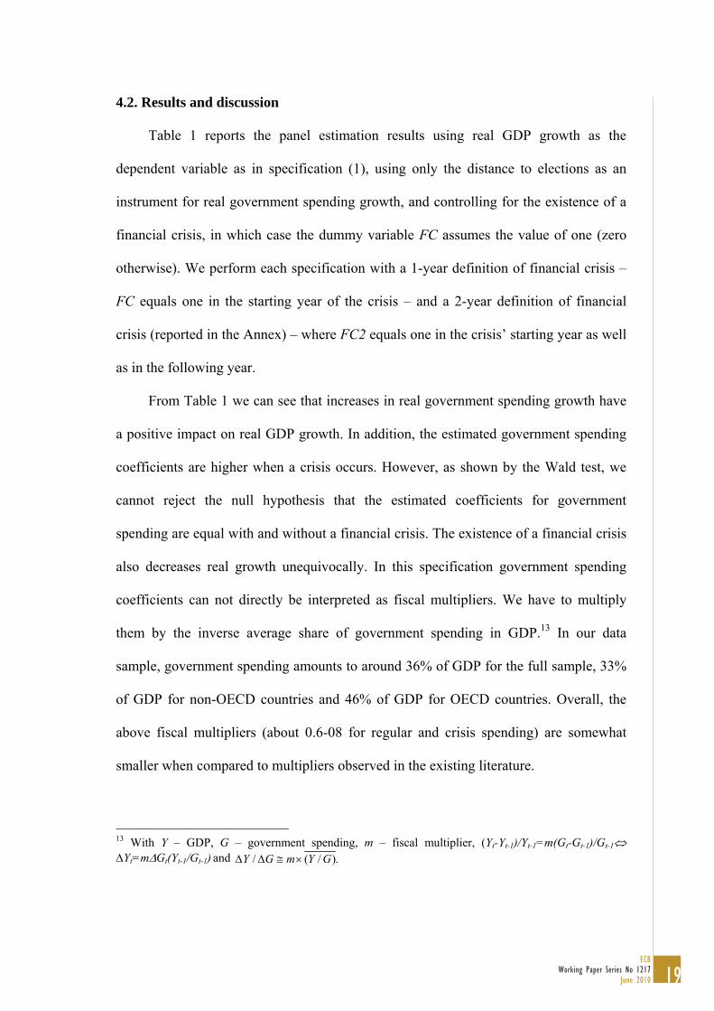
4.2. Results and discussion
Table 1 reports the panel estimation results using real GDP growth as the
dependent variable as in specification (1), using only the distance to elections as an
instrument for real government spending growth, and controlling for the existence of a
financial crisis, in which case the dummy variable FC assumes the value of one (zero
otherwise). We perform each specification with a 1-year definition of financial crisis –
FC equals one in the starting year of the crisis – and a 2-year definition of financial
crisis (reported in the Annex) – where FC2 equals one in the crisis’ starting year as well
as in the following year.
From Table 1 we can see that increases in real government spending growth have
a positive impact on real GDP growth. In addition, the estimated government spending
coefficients are higher when a crisis occurs. However, as shown by the Wald test, we
cannot reject the null hypothesis that the estimated coefficients for government
spending are equal with and without a financial crisis. The existence of a financial crisis
also decreases real growth unequivocally. In this specification government spending
coefficients can not directly be interpreted as fiscal multipliers. We have to multiply
them by the inverse average share of government spending in GDP.13 In our data
sample, government spending amounts to around 36% of GDP for the full sample, 33%
of GDP for non-OECD countries and 46% of GDP for OECD countries. Overall, the
above fiscal multipliers (about 0.6-08 for regular and crisis spending) are somewhat
smaller when compared to multipliers observed in the existing literature.
13 With Y – GDP, G – government spending, m – fiscal multiplier, (Yt-Yt-1)/Yt-1=m(Gt-Gt-1)/Gt-1 Yt=mGt(Yt-1/Gt-1) and / ( / ).Y G m Y G

20ECBWorking Paper Series No 1217June 2010
Table 1 – Results for real GDP growth (1981-2007), spending growth rates, instrument: distance to elections, 1-year crisis
(1) (2) (3) (4) Spending*(1-FC) 0.322* 0.228* 0.180 0.0858 (1.89) (1.70) (1.24) (0.68) Spending*FC 0.642 0.489* 0.428* 0.601 (1.10) (1.93) (1.80) (1.60) GDP(-1) 0.197 0.243*** 0.242** 0.142* (1.58) (2.66) (2.49) (1.73) FC -0.0797** -0.0869*** -0.0909*** (dropped) (-2.17) (-3.89) (-4.36) FC(-1) 0.000166 -0.000828 -0.00112 -0.00618 (0.03) (-0.15) (-0.22) (-1.20) Spending(-1)*(1-FC(-1)) 0.00586 0.00472 0.00541 (0.33) (0.26) (0.33) Spending(-1)*FC(-1) 0.0645 0.0583 0.0700 (1.49) (1.41) (1.05) Revenue(-1) 0.00815 0.0139 0.0246 (0.33) (0.54) (1.33) Claims on Private Sector 0.0168*** (2.65) Inflation -0.00261** (-2.20) Time Fixed Effects No No Yes Yes Observations 2605 2516 2516 1937 Cross-sections 122 122 122 101 Kleibergen-Paap LM Statistic 6.91 8.10 6.41 5.35 Kleibergen-Paap p-value 0.0086 0.0044 0.0113 0.0207 Wald Test Statistic 0.28 0.87 0.80 1.57 Wald Test p-value 0.5959 0.3502 0.3719 0.2096
Notes: unbalanced panels with country fixed effects. t-statistics are in brackets. *, ** and *** denote level of significance indicating 10%, 5% and 1% respectively. A Wald test is conducted to test whether crisis spending and regular spending are statistically different. The underlying null hypothesis of the test is that the coefficients of the interaction terms between spending and financial crisis are equal. GDP, Spending, Revenue and Claims on Private Sector are used as growth rates. FC – dummy variable for the existence of financial crisis. The Kleibergen-Paap statistic tests the null that the equation is underidentified. Constant as well as fixed effects interactions with crises dummy are partialled out.
Similar results can be observed when government spending is instrumented with
both the distance to elections and the lagged budget balance (see Table 2). In this case,
the fiscal multiplier is around 0.8. In addition, both with one and with two instruments,
we can see that claims to the private sector have a positive estimated coefficient,
implying that increases in credit concession to the private sector can positively impinge
on economic growth (see last columns of tables 1 and 2).

21ECB
Working Paper Series No 1217June 2010
Our sample comprises observations from a diverse set of countries and thus
collects information from very heterogeneous financial crises. To allow for a different
severity of crisis across countries and a reaction of economic variables to the occurrence
of financial crisis (possibly due, for instance, to institutional differences) we interact
country dummies with crisis dummies in each specification.
Table 2 – Results for real GDP growth (1981-2007), spending growth rates, instrument: distance to elections and lagged budget balance, 1-year crisis
(1) (2) (3) (4) Spending*(1-FC) 0.151*** 0.291** 0.251** 0.192 (2.95) (2.48) (2.20) (1.36) Spending*FC 0.128 0.263** 0.256** 0.140 (1.60) (2.13) (2.12) (1.09) GDP(-1) 0.307*** 0.226*** 0.216*** 0.117 (5.68) (2.92) (2.81) (1.40) GDP(-2) 0.0190 0.0227 0.0237 0.00771 (0.53) (0.64) (0.69) (0.22) FC -0.111*** -0.104*** -0.105*** (-5.79) (-5.40) (-5.53) FC(-1) -0.00835** -0.00418 -0.00427 -0.00747 (-2.06) (-0.85) (-0.92) (-1.42) Budget balance ratio(-2) -0.0315 -0.113 -0.0991 -0.134 (-1.24) (-1.48) (-1.40) (-1.40) Spending(-1)*(1-FC(-1)) 0.0367 0.0310 0.0375 (1.28) (1.15) (1.11) Spending(-1)*FC(-1) 0.0533 0.0487 0.00794 (1.01) (0.96) (0.11) Revenue(-1) -0.0163 -0.00886 -0.00289 (-0.66) (-0.38) (-0.12) Claims on Private Sector 0.0165*** (3.10) Inflation -0.00193*** (-4.13) Time Fixed Effects No No Yes Yes Observations 2504 2439 2439 1884 No. Clusters 122 122 122 101 Kleibergen-Paap LM Statistic 26.14 13.80 14.31 9.22 Kleibergen-Paap p-value 0.0000 0.0032 0.0025 0.0264 Wald Test Statistic 0.07 0.09 0.00 0.14 Wald Test p-value 0.7931 0.7691 0.9596 0.7090
Notes: unbalanced panels with country fixed effects. t-statistics are in brackets. *, ** and *** denote level of significance indicating 10%, 5% and 1% respectively. A Wald test is conducted to test whether crisis spending and regular spending are statistically different. The underlying null hypothesis of the test is that the coefficients of the interaction terms between spending and financial crisis are equal. GDP, Spending, Revenue and Claims on Private Sector are used as growth rates. FC – dummy variable for the existence of financial crisis. The Kleibergen-Paap statistic tests the null that the equation is underidentified. Equation (4) is over-identified. Constant as well as fixed effects interactions with crises dummy are partialled out.

22ECBWorking Paper Series No 1217June 2010
The above results from the IV regression with “differentiated fixed effects” are
similar to the results obtained with a sample split into crises and non-crises
observations.14 By keeping the full sample and introducing a country specific
interaction term with crises we benefit from gains in efficiency and instrument validity.
Moreover, we can directly test the hypothesis of equality between spending in crises
and non-crises times.15
A direct consequence of this approach is that – as in the case of fixed effects –
observations for countries with only one crisis-year (singleton dummies) are not
included in the analysis. Since many countries indeed experienced several financial
crises, our FC dummy variable captures 111 crises years for 45 countries with 2 to 4
crises. The coefficient of the FC dummy in the tables has to be interpreted by taking
into account that country specific crises reactions of GDP have already been partialled
out. For robustness, we run every specification with a 2-year definition of crises, which
also includes observations with only one crisis per country (see Annex).
Instrument Performance
In Tables 1 and 2 we can reject the null hypothesis that the equation is
underidentified. In Table 2, including the lagged budget ratio balance improves the
instrument performance in the first stage for crisis spending. Indeed, the Kleibergen-
Paap test statistic also passes the critical value of 10 allowing rejecting the null of
underidentification.
14 Tables are not reported and can be obtained from the authors upon request. 15 The coefficients of these interaction terms are not reported since they are partialled out in the regressions, together with the constant.

23ECB
Working Paper Series No 1217June 2010
Therefore, regular distance to elections and regular lagged budget balance ratios
are good predictors for regular spending. The closer to elections, the higher is spending
growth. The larger the buffer provided by last year’s budget balance position relative to
last year’s GDP, the higher is government spending growth during normal times. The
instrument lagged budget balance has a similar performance during financial crises as
during regular times: there is a significant and positive correlation between regular
spending and regular lagged budget balance. Distance to elections, however, changes
the sign such that the political budget cycle during crises is positively correlated with
crisis spending and is weakly (1-year crisis) to highly (2-year crisis, see Annex)
significant. The further away elections are, the more the government is reacting via
spending during crisis.16
Fiscal Multipliers
According to the results in Table 1 and 2 the fiscal multiplier for instrumented
regular spending ranges between 0.6 and 1.1 assuming an average government spending
share of GDP of about one third.17 In addition, reverse causality seems to be stronger in
crisis times. Indeed, our results show a somewhat larger marginal impact for crisis
spending. Intuitively, this is appealing, implying that social transfers and discretionary
spending react stronger during an expected and/or experienced economic downturn than
in times of an economic upswing. Overall, albeit the qualitative differences,
endogeneity does not influence our findings since the marginal impact of spending is
not statistically different in crisis and non-crisis times.
16 Exogeneity tests rejected the hypothesis that a fall in GDP leads to new elections, hence we reject the hypothesis that the instrument is correlated with the dependent variable. 17 Our estimates based on different instruments yield output multipliers that are close to the ones derived, for instance, in the papers by Baxter and King (1993), Linnemann and Schabert (2003).

24ECBWorking Paper Series No 1217June 2010
Moreover, government spending in the presence of a financial crisis, when
compared to normal times, is clearly larger in Table 1 compared to Table 2. This is
likely to be due to a weak instrument bias for crisis spending when using only the
distance to elections indicator (see above). Including the lagged budget balance ratio,
the coefficients of crisis spending and regular spending are approximately equal.
4.3. Robustness analysis
OECD and non-OECD economies
Evidence from the related literature points out that (economic) cyclical fiscal
behaviour in developed economies is somewhat different from the case of developing
economies. The conventional wisdom that emerges from such studies is that fiscal
policy is counter-cyclical or a-cyclical in most developed countries, while it is pro-
cyclical in developing countries.18 More specifically, reverse causality could be
different in developed and developing economies. It is therefore important to analyse
the instrument’s performance and instrumented fiscal multipliers in OECD and non-
OECD sub-samples.
As Table 3 shows, the results for non-OECD countries are close to the results
obtained for the full sample and fiscal multipliers, for both crisis and regular spending,
are on average 0.6. In addition, the instruments behave similarly in the first stage and
statistical significance is even stronger compared to the full sample regressions.
For OECD countries, however, distance to elections, i.e. the political budget
cycle, does not perform very well as an instrument during regular times (see Table 4).
18 See, for instance, Galí (1994), Lane (2003), Kaminsky et al. (2004), Talvi and Vegh (2005), and Alesina et al. (2008)

25ECB
Working Paper Series No 1217June 2010
Table 3 – Results for real GDP growth (1981-2007), spending growth rates, instrument: distance to elections and lagged budget balance, non-OECD countries, 1-year crisis
(1) (2) (3) (4) Spending*(1-FC) 0.153*** 0.258** 0.218** 0.177 (3.08) (2.48) (2.18) (1.53) Spending*FC 0.137* 0.258** 0.237* 0.170 (1.65) (1.97) (1.90) (1.33) GDP(-1) 0.295*** 0.229*** 0.218*** 0.0951 (5.08) (2.99) (2.96) (1.26) GDP(-2) 0.0329 0.0376 0.0295 0.0147 (0.83) (0.98) (0.80) (0.40) FC -0.111*** -0.104*** -0.105*** (dropped) (-5.72) (-5.33) (-5.47) FC(-1) -0.00756* -0.00301 -0.00337 -0.00579 (-1.66) (-0.56) (-0.68) (-0.98) Budget balance ratio(-2) -0.0324 -0.102 -0.0825 -0.160 (-0.96) (-1.20) (-1.08) (-1.39) Spending*(1-FC(-1)) 0.0332 0.0253 0.0422 (1.14) (0.93) (1.17) Spending*FC(-1) 0.0545 0.0476 0.0268 (1.03) (0.93) (0.39) Revenue(-1) -0.0121 -0.00362 -0.00673 (-0.50) (-0.16) (-0.26) Claims on Private Sector 0.0168** (2.32) Inflation -0.00204*** (-4.33) Time Fixed Effects No No Yes Yes Observations 1814 1750 1750 1261 Cross-sections 94 94 94 73 Kleibergen-Paap LM Statistic 26.99 15.79 16.36 12.42 Kleibergen-Paap p-value 0.0000 0.0013 0.0010 0.0061 Wald Test Statistic 0.04 0.00 0.04 0.00 Wald Test p-value 0.8479 0.9969 0.8329 0.9568
Notes: unbalanced panels with country fixed effects. t-statistics are in brackets. *, ** and *** denote level of significance indicating 10%, 5% and 1% respectively. A Wald test is conducted to test whether crisis spending and regular spending are statistically different. The underlying null hypothesis of the test is that the coefficients of the interaction terms between spending and financial crisis are equal. GDP, Spending, Revenue and Claims on Private Sector are used as growth rates. FC – dummy variable for the existence of financial crisis. The Kleibergen-Paap statistic tests the null that the equation is underidentified. Constant as well as fixed effects interactions with crises dummy are partialled out.

26ECBWorking Paper Series No 1217June 2010
Table 4 – Results for real GDP growth (1981-2007), spending growth rates, instrument: distance to elections and lagged budget balance, OECD countries, 1-year crisis
(1) (2) (3) (4) Spending*(1-FC) 0.784 1.029 0.719 -0.0415 (1.00) (0.85) (1.09) (-0.15) Spending*FC 0.303*** 0.327** 0.284* 0.216* (2.65) (1.99) (1.79) (1.73) GDP(-1) 0.121 -0.00886 0.0932 0.411*** (0.32) (-0.02) (0.26) (4.03) GDP(-2) -0.135 -0.141* -0.0971 -0.0642 (-1.55) (-1.65) (-1.44) (-1.29) FC (dropped) 0.0488*** (dropped) (dropped) (3.87) FC(-1) -0.0314 -0.0379 -0.0336 -0.00437 (-1.08) (-0.83) (-1.05) (-0.28) Budget balance ratio(-2) -0.135 -0.237 -0.167 -0.00491 (-0.99) (-0.90) (-1.20) (-0.06) Spending*(1-FC(-1)) -0.0234 0.0138 0.0364* (-0.46) (0.32) (1.78) Spending*FC(-1) -0.0410 0.161 -0.0359 (-0.10) (0.43) (-0.20) Revenue(-1) 0.0213 -0.00359 0.00969 (0.26) (-0.06) (0.35) Claims on Private Sector 0.00730 (1.39) Inflation -0.0198* (-1.81) Time Fixed Effects No No Yes Yes Observations 690 689 689 623 Cross-sections 28 28 28 28 Kleibergen-Paap LM Statistic 2.69 0.68 1.11 3.68 Kleibergen-Paap p-value 0.4423 0.8775 0.7740 0.2977 Wald Test Statistic 0.32 0.37 0.48 1.12 Wald Test p-value 0.5702 0.5448 0.4907 0.2907
Notes: unbalanced panels with country fixed effects. t-statistics are in brackets. *, ** and *** denote level of significance indicating 10%, 5% and 1% respectively. A Wald test is conducted to test whether crisis spending and regular spending are statistically different. The underlying null hypothesis of the test is that the coefficients of the interaction terms between spending and financial crisis are equal. GDP, Spending, Revenue and Claims on Private Sector are used as growth rates. FC – dummy variable for the existence of financial crisis. The Kleibergen-Paap statistic tests the null that the equation is underidentified. Constant as well as fixed effects interactions with crises dummy are partialled out.
Literature on the political budget cycle mostly confirms our results of different
fiscal attitudes in OECD and non-OECD countries (see, for instance, Shi and Svensson,
2006). Interestingly, distance to elections matters for crisis spending as we find a
significant negative correlation in the first stage. In other words, during financial crisis,
fiscal action is required by the electorate in OECD countries. The lagged budget

27ECB
Working Paper Series No 1217June 2010
balance-to-GDP ratio is also significant during crisis with a clearly larger coefficient
than in the non-OECD countries regressions, while it is not significant in regular times.
Overall, it proved to be difficult to build a significant instrument for regular
spending in OECD countries. Therefore, in Table 4 (and 4b in the Annex) the under
identification test is not passed. The reported value, however, only captures the average
validity of instruments over both endogenous variables. The instruments for crisis
spending, crisis distance to elections and crisis lagged budget balance, are still highly
significant in the first stage. The fiscal multiplier of crisis spending ranges between 0.5
and 0.7 and is therefore slightly larger than in non-OECD countries (the underlying
fiscal share is 46% of GDP, as described above).
Banking crisis
The previous analysis showed the impact of government spending on economic
growth during up to 141 financial crises, which included banking crises, currency crises,
and debt crises. Table 5 reports on to which extent government spending and growth are
correlated during 60 banking crises.
Given the limited number of banking crises recorded in the IMF dataset on
financial crisis, between 1981 and 2007 and, in particular, the high proportion of only
one banking crises per country, we can only use the 2-year definition of crises, which
provides us with two observations per crisis and thus allows us to use the singleton
crises. Again, country dummies are interacted with banking crisis dummy in
specifications (1)-(3) in Table 5, hence the coefficient of BC2 has to be interpreted
taking into account the country specific crises reactions. Without interactions, BC2 is
significantly negative, as in regression (1).
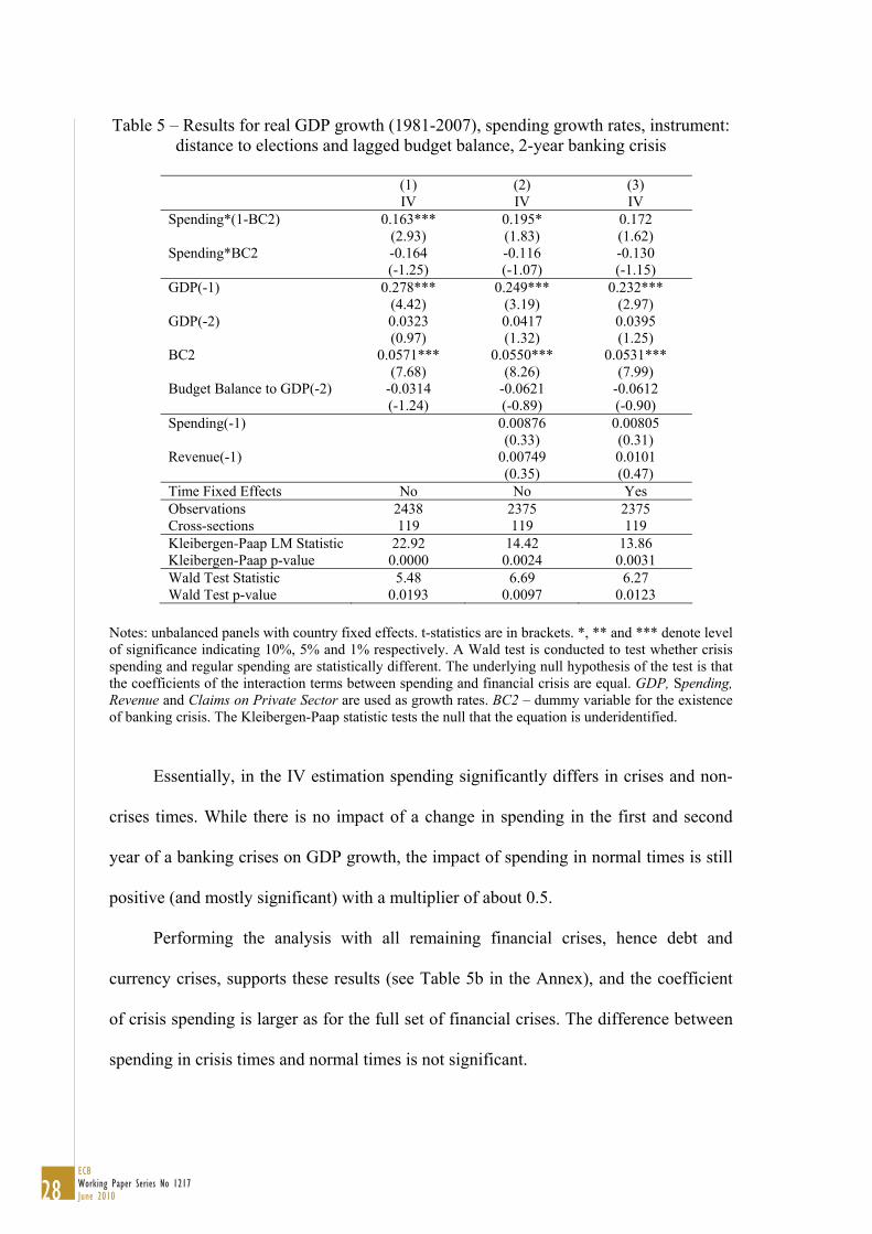
28ECBWorking Paper Series No 1217June 2010
Table 5 – Results for real GDP growth (1981-2007), spending growth rates, instrument: distance to elections and lagged budget balance, 2-year banking crisis
(1) (2) (3) IV IV IV Spending*(1-BC2) 0.163*** 0.195* 0.172 (2.93) (1.83) (1.62) Spending*BC2 -0.164 -0.116 -0.130 (-1.25) (-1.07) (-1.15) GDP(-1) 0.278*** 0.249*** 0.232*** (4.42) (3.19) (2.97) GDP(-2) 0.0323 0.0417 0.0395 (0.97) (1.32) (1.25) BC2 0.0571*** 0.0550*** 0.0531*** (7.68) (8.26) (7.99) Budget Balance to GDP(-2) -0.0314 -0.0621 -0.0612 (-1.24) (-0.89) (-0.90) Spending(-1) 0.00876 0.00805 (0.33) (0.31) Revenue(-1) 0.00749 0.0101 (0.35) (0.47) Time Fixed Effects No No Yes Observations 2438 2375 2375 Cross-sections 119 119 119 Kleibergen-Paap LM Statistic 22.92 14.42 13.86 Kleibergen-Paap p-value 0.0000 0.0024 0.0031 Wald Test Statistic 5.48 6.69 6.27 Wald Test p-value 0.0193 0.0097 0.0123
Notes: unbalanced panels with country fixed effects. t-statistics are in brackets. *, ** and *** denote level of significance indicating 10%, 5% and 1% respectively. A Wald test is conducted to test whether crisis spending and regular spending are statistically different. The underlying null hypothesis of the test is that the coefficients of the interaction terms between spending and financial crisis are equal. GDP, Spending, Revenue and Claims on Private Sector are used as growth rates. BC2 – dummy variable for the existence of banking crisis. The Kleibergen-Paap statistic tests the null that the equation is underidentified.
Essentially, in the IV estimation spending significantly differs in crises and non-
crises times. While there is no impact of a change in spending in the first and second
year of a banking crises on GDP growth, the impact of spending in normal times is still
positive (and mostly significant) with a multiplier of about 0.5.
Performing the analysis with all remaining financial crises, hence debt and
currency crises, supports these results (see Table 5b in the Annex), and the coefficient
of crisis spending is larger as for the full set of financial crises. The difference between
spending in crisis times and normal times is not significant.

29ECB
Working Paper Series No 1217June 2010
5. Conclusion
In this paper we have studied the impact of government spending on output
notably during the occurrence of financial crises, covering 127 countries for the period
1981-2007. We have performed each estimation using a 1-year and a 2-year definition
of financial crisis, with and without time fixed effects.
To address the endogeneity issue we have used two instruments: the distance to
elections – a linear distance measure between the current year and the year of the next
election – and the lagged budget balance-to-GDP ratio. According to the results, the
fiscal multiplier for instrumented regular spending ranges between 0.6 and 0.8,
considering the average government spending share of GDP of about one third. The
multipliers of instrumented government spending are higher than the simple OLS
multipliers. However, the differences between the coefficients of government spending
in crises and non-crises periods are also insignificant in most of our estimations.
More specifically, the fiscal multiplier for the full sample and for the non-OECD
sub-sample, for instrumented regular and crisis government spending, is about 0.6, with
an average government spending-to-GDP ratio of one third. For the OECD sub-sample,
government spending in the presence of a financial crisis also produces a fiscal
multiplier of 0.6 assuming an average fiscal share of GDP of around 40 percent.
Moreover, for the sub-sets of OECD and non-OECD countries our results show, that
altogether, we also cannot reject the hypothesis that government spending either in the
presence or in the absence of a financial crisis has the same impact. Interestingly, for the
cases when a banking crisis occurred, our results do not support the idea that
expansionary fiscal policies positively impact on economic growth.

30ECBWorking Paper Series No 1217June 2010
Therefore, the main result of our panel analysis is that that government spending
has essentially the same impact on economic growth with or without a financial crisis.
This result holds throughout our sample, using a variation of controls, sub-samples and
specifications. Consequently, taking into account that larger spending programmes tend
to be less targeted, this indicates that they may actually not be particularly helpful.
The present analysis is a first step and these conclusions are tentative. Additional
research is needed to further study the relevance of fiscal policies in the context of
financial crisis. One way forward would be to use more detailed data on the
composition of government spending and to distinguish between budgetary components
that react to changes in output and others that don’t.
References
Afonso, A. (2010). “Expansionary fiscal consolidations in Europe: new evidence”,
Applied Economics Letters, 17 (2), 105-109.
Afonso, A., Claeys, P. (2007). “The dynamic behaviour of budget components and
output”, Economic Modelling, 25 (1), 93-117.
Afonso, A. and Furceri, D. (2010). “Government size, composition, volatility and
economic growth,” European Journal of Political Economy, forthcoming.
Afonso, A. and González Alegre, J. (2008). “Economic Growth and Budgetary
Components: a Panel Assessment for the EU,” ECB Working Paper 848.
Afonso, A. and Sousa, R. (2009). “The Macroeconomic Effects of Fiscal Policy,” ECB
Working Paper 991.
Alesina, A., Campante, F. and Tabellini, G. (2008). “Why is Fiscal Policy Often
Procyclical?” Journal of the European Economic Association, 6 (5), 1006-1036.
Baldacci, E., Gupta, S. and Mulas-Granados, C. (2009). “How Effective is Fiscal
Policy Response in Systemic Banking Crises?”, IMF Working Paper 09/160.
Baxter, M. and King, R. (1993). “Fiscal policy in general equilibrium”, American
Economic Review, 83 (3), 315–334.

31ECB
Working Paper Series No 1217June 2010
Bénassy, J.-P. (1986). Macroeconomics: An Introduction to the Non-Walrasian
Approach, Academic Press, Orlando, FL.
Bénassy-Quéré, A. and Cimadomo, J. (2006). “Changing Patterns of Domestic and
Cross-Border Fiscal Policy Multipliers in Europe and the US”, CEPII Working
Paper 200-24.
Bernanke, B., Gertler, M. and Gilchrist, S. (2000). “The Financial Accelerator in a
Quantitative Business Cycle Framework,” in Taylor, J. and Woodford, M. (eds.)
Handbook of Macroeconomics, vol. 1C. Elsevier.
Blanchard, O. (2008). “The Tasks Ahead”, IMF Working Paper 08/262.
Blanchard, O. and Perotti, R. (2002). “An Empirical Characterization of the Dynamic
Effects of Changes in Government Spending and Taxes on Output”, Quarterly
Journal of Economics, 117 (4), 1329-1368.
Brender, A. and Drazen, A. (2005). “Political budget cycles in new versus established
democracies”, Journal of Monetary Economics, 52 (5), 1271-1295.
Cerra, V. and Saxena, S. (2008). “Growth Dynamics: The Myth of Economic
Recovery,” American Economic Review, 98 (1), 439–457.
Claessens, S., Kose, A. and Terrones, M. (2008). “What Happens During Recessions,
Crunches and Busts?” CEPR Discussion Paper N. 7085.
Cogan, J., Cwik, T.; Taylor, J. and Wieland, V. (2009). “New Keynesian versus Old
Keynesian Government Spending Multipliers”, NBER Working Paper 14782.
De Arcangelis, G. and Lamartina, S. (2003). ”Identifying Fiscal Shocks and Policy
Regimes in OECD Countries”, ECB Working Paper 281.
Fatás, A. and Mihov, I. (2001). “The Effects of Fiscal Policy on Consumption and
Employment: Theory and Evidence”, INSEAD, mimeo.
Forni, L., Monteforte, L. and Sessa, L. (2009). “The General Equilibrium Effects of
Fiscal Policy: Estimates for the Euro Area”, Journal of Public Economics, 93 (3-4),
559-585.
Galí, J. (1994). “Government Size and Macroeconomic Stability”, European Economic
Review, 38(1), 117-32.
Galí, J., Lopez-Salido, J. and Valles, J. (2007). “Understanding the Effects of
Government Spending on Consumption”, Journal of the European Economic
Association, 5 (1), 227-270.

32ECBWorking Paper Series No 1217June 2010
Giavazzi, F. and Pagano, M. (1990). “Can Severe Fiscal Contractions be Expansionary?
Tales of Two Small European Countries”, in Blanchard, O. and Fischer, S. (eds.),
NBER Macroeconomics Annual 1990, MIT Press.
Hibbs, D. (1977). “Political Parties and Macroeconomic Policy”, American Political
Science Review. 7, 1467-1487.
IMF (2009). “The State of Public Finances: Outlook and Medium-Term Policies After
the 2008 Crisis”, IMF March 2009.
Jaeger, A. and Schuknecht, L. (2004). “Boom-Bust Phases in Asset Prices and Fiscal
Policy Behavior,” IMF Working Paper 04/54.
Johnson, D., Parker, J., and Souleles, N. (2006). “Household Expenditure and the
Income Tax Rebates of 2001”, American Economic Review 96 (5), 1589-1610.
Kaminsky, G., Reinhart, C. and Végh, C. (2004). “When It Rains, It Pours: Procyclical
Capital Flows and Macroeconomic Policies”, NBER Working Paper 10780.
Krugman, P. (2005). “Is Fiscal Policy Poised for a Comeback?” Oxford Review of
Economic Policy, 21 (4), 515-523.
Laeven, L. and Valencia, F. (2008). “Systemic Banking Crises: A New Database”, IMF
Working Paper 08/224.
Lane, P. (2003). “The cyclical behaviour of fiscal policy: evidence from the OECD”,
Journal of Public Economics, 87(12), 2261-2675.
Linnemann, L. and Schabert, A. (2003) “Fiscal policy and the new neoclassical
synthesis”, Journal of Money, Credit and Banking, 35 (6), 911–929.
Malinvaud, E. (1985). The Theory of Unemployment Reconsidered, Oxford: Basil
Blackwell.
Nordhaus, W. (1975). “The Political Business Cycle”, Review of Economic Studies. 42,
169-190.
OECD (2009). OECD Economic Outlook, Interim Report March 2009.
Perotti, R. (2004). “Estimating the Effects of Fiscal Policy in OECD Countries”. CEPR
Discussion Paper 168. Center for Economic Policy Research, London.
Ramey, V. and Shapiro, M. (1998). “Costly capital reallocation and the effects of
government spending”, Carnegie Rochester Conference on Public Policy, 48, 145-
194.

33ECB
Working Paper Series No 1217June 2010
Ratto, M., Roeger, W. and in 't Veld, J. (2008). “QUEST III: An Estimated Open-
Economy DSGE Model of the Euro Area with Fiscal and Monetary Policy”,
Economic Modelling, 26 (1), 222-233.
Röger W., Székely, I. and Turrini, A. (2010). “Banking crises, Output Loss and Fiscal
Policy”. CEPR Discussion paper 7815.
Shi, M., and J. Svensson (2006). “Political budget cycles: Do they differ across
countries and why?”, Journal of Public Economics, 90, 1367-1389.
Spilimbergo, A., Symansky, S., Blanchard, O. and Cottarelli, C. (2008). “Fiscal Policy
for the Crisis”, IMF Staff Position Note SPN/08/01.
Tagkalakis, A (2008). “The effects of fiscal policy on consumption in recessions and
expansions”, Journal of Public Economics, 92 (5-6), 1486-1508.
Talvi, E. and Vegh, C. (2005). “Tax base variability and procyclical fiscal policy”,
Journal of Economic Development, 78(1), 156-190.
Van Brusselen, P. (2010). “Fiscal Stabilisation Plans andthe Outlook for the World
Economy”, mimeo, Banca d’Italia’s 12th Public Finance Workshop on “Fiscal
Policy: Lessons from the Crisis”, Perugia, 25-27 March, 2010.

34ECBWorking Paper Series No 1217June 2010
Appendix – Data description and sources
Non-performing loans: data available on the website of Luc Laeven, reported as a
percentage of GDP at the peak of a crisis. http://www.luclaeven.com/Data.htm
Year of crisis: banking, currency or sovereign debt crisis. Source: IMF database on
financial crises, Laeven and Valencia (2008), and at
http://www.luclaeven.com/Data.htm
Government spending: general government spending deflated with the GDP deflator.
For some countries only central government data are available. Source: IMF World
Economic Outlook database.
Budget balance: general government budget balance as percent of GDP. For some
countries only central government data are available. Source: IMF World Economic
Outlook database.
Government debt: government gross debt as percent of GDP. For some countries only
central government data are available. Source: IMF World Economic Outlook
database.
Real GDP: Source: IMF World Economic Outlook database.
GDP gap: difference between actual and trend real GDP, as a percentage of trend real
GDP. Trend GDP is estimated using an HP-filter on real GDP. The lambda value is
chosen as 100.
Inflation rate: Consumer price index. Source: IMF World Economic Outlook database
Long-term nominal interest rate: Data are only available for OECD countries. Source:
OECD Economic Outlook database.
Election dates: Legal and Executive Elections taken from Pippa Norris. 2009.
Democracy Time series Dataset.
http://www.hks.harvard.edu/fs/pnorris/Data/Data.htm

35ECB
Working Paper Series No 1217June 2010
List of countries
All countries OECD sub-sample Albania Ghana Oman Australia Algeria Greece Pakistan Austria Antigua and Barbuda Guinea Panama Belgium Argentina Guinea-Bissau Paraguay Canada Australia Guyana Peru Czech Republic Austria Hungary Philippines Denmark Azerbaijan Iceland Poland Finland Bahamas, The India Portugal France Bangladesh Indonesia Romania Germany Barbados Iran Russia Greece Belgium Ireland São Tomé and Príncipe Hungary Belize Israel Saudi Arabia Iceland Bolivia Italy Senegal Ireland Bosnia and Herzegovina Jamaica Seychelles Italy Brazil Japan Singapore Japan Bulgaria Jordan Slovak Republic Korea Burkina Faso Kazakhstan Slovenia Luxembourg Burundi Kenya South Africa Mexico Cambodia Korea Spain Netherlands Canada Kuwait Sri Lanka New Zealand Cape Verde Kyrgyz Republic Swaziland Norway Chile Lao Sweden Poland China Latvia Switzerland Portugal Colombia Lebanon Syrian Arab Republic Slovak Republic Costa Rica Lithuania Taiwan Spain Côte d'Ivoire Luxembourg Tajikistan Sweden Croatia Madagascar Thailand Switzerland Cyprus Malaysia Trinidad and Tobago United Kingdom Czech Republic Mauritania Turkmenistan United States Denmark Mauritius Uganda Djibouti Mexico Ukraine Dominican Republic Moldova United Arab Emirates Ecuador Mongolia United Kingdom Egypt Morocco United States El Salvador Mozambique Uruguay Equatorial Guinea Namibia Uzbekistan Estonia Nepal Venezuela Ethiopia Netherlands Vietnam Fiji New Zealand Yemen Finland Nicaragua Zambia France Niger Zimbabwe Georgia Nigeria Germany Norway

36ECBWorking Paper Series No 1217June 2010
Annex – Additional results
Table 1b – Results for real GDP growth (1981-2007), spending growth rates,
instrument: distance to elections, 2-year crisis
(1) (2) (3) (4) Spending*(1-FC2) 0.337** 0.275** 0.212* 0.146 (2.32) (2.26) (1.68) (1.40) Spending*FC2 0.512 0.399 0.339 0.271 (1.17) (1.53) (1.41) (1.42) GDP(-1) 0.131 0.160* 0.171** 0.0689 (1.29) (1.90) (2.02) (0.91) FC2 -0.0841*** -0.0837*** -0.0789*** (-12.90) (-20.14) (-16.93) Spending(-1) 0.0203 0.0178 0.00712 (1.00) (0.90) (0.47) Revenue(-1) 0.000643 0.00608 0.0166 (0.03) (0.31) (1.14) Claims on Private Sector 0.0150*** (2.76) Inflation -0.00222*** (-3.09) Time Fixed Effects No No Yes Yes Observations 2605 2516 2516 1937 Cross-sections 122 122 122 101 Kleibergen-Paap LM Statistic 11.05 12.12 10.68 9.47 Kleibergen-Paap p-value 0.0009 0.0005 0.0011 0.0021 Wald Test Statistic 0.14 0.20 0.22 0.35 Wald Test p-value 0.7040 0.6575 0.6400 0.5555
Notes: unbalanced panels with country fixed effects. t-statistics are in brackets. *, ** and *** denote level of significance indicating 10%, 5% and 1% respectively: A Wald test is conducted to test whether crisis spending and regular spending are statistically different. The underlying null hypothesis of the test is that the coefficients of the interaction terms between spending and financial crisis are equal. . GDP, Spending, Revenue and Claims on Private Sector are used as growth rates. FC2 – dummy variable for the existence of financial crisis. The Kleibergen-Paap statistic tests the null that the equation is underidentified. Constant as well as fixed effects interactions with crises dummy are partialled out.

37ECB
Working Paper Series No 1217June 2010
Table 2b – Results for real GDP growth (1981-2007), spending growth rates, instrument: distance to elections and lagged budget balance, 2-year crisis
(1) (2) (3) (4) Spending*(1-FC2) 0.164*** 0.262** 0.224** 0.207* (2.80) (2.38) (2.11) (1.82) Spending*FC2 0.0692 0.181* 0.175* 0.105 (0.95) (1.75) (1.70) (1.14) GDP(-1) 0.257*** 0.193*** 0.183** 0.0782 (4.73) (2.68) (2.55) (1.05) GDP(-2) 0.0329 0.0414 0.0450 0.0240 (1.03) (1.33) (1.52) (0.78) FC2 -0.0814*** -0.0836*** -0.0786*** (-54.12) (-40.78) (-23.58) Budget balance ratio(-2) -0.0232 -0.0898 -0.0795 -0.141* (-0.82) (-1.25) (-1.20) (-1.79) Spending(-1) 0.0291 0.0253 0.0259 (1.10) (0.98) (0.86) Revenue(-1) -0.00708 -0.00240 -0.00141 (-0.34) (-0.12) (-0.07) Claims on Private Sector 0.0158*** (3.23) Inflation -0.00203*** (-3.88) Time Fixed Effects No No Yes Yes Observations 2504 2439 2439 1884 No. Clusters 122 122 122 101 Kleibergen-Paap LM Statistic 25.54 15.53 16.71 13.60 Kleibergen-Paap p-value 0.0000 0.0014 0.0008 0.0035 Wald Test Statistic 1.08 0.55 0.21 1.19 Wald Test p-value 0.2995 0.4592 0.6488 0.2753
Notes: unbalanced panels with country fixed effects. t-statistics are in brackets. *, ** and *** denote level of significance indicating 10%, 5% and 1% respectively. A Wald test is conducted to test whether crisis spending and regular spending are statistically different. The underlying null hypothesis of the test is that the coefficients of the interaction terms between spending and financial crisis are equal. . GDP, Spending, Revenue and Claims on Private Sector are used as growth rates. FC2 – dummy variable for the existence of financial crisis. The Kleibergen-Paap statistic test the null that the equation is underidentified. Constant as well as fixed effects interactions with crises dummy are partialled out.

38ECBWorking Paper Series No 1217June 2010
Table 3b – Results for real GDP growth (1981-2007), spending growth rates, instrument: distance to elections and lagged budget balance, non-OECD countries, 2-
year crisis
(1) (2) (3) (4) Spending*(1-FC2) 0.168*** 0.248** 0.203** 0.192** (2.99) (2.54) (2.17) (2.05) Spending*FC2 0.0985 0.209** 0.183* 0.147 (1.47) (2.08) (1.85) (1.49) GDP(-1) 0.239*** 0.180** 0.174** 0.0478 (4.15) (2.48) (2.47) (0.67) GDP(-2) 0.0467 0.0588* 0.0513 0.0328 (1.33) (1.74) (1.61) (0.98) FC2 -0.0821*** -0.0847*** -0.0771*** (-54.66) (-36.37) (-18.50) Budget balance ratio(-2) -0.0204 -0.0870 -0.0663 -0.174* (-0.55) (-1.07) (-0.92) (-1.77) Spending(-1) 0.0306 0.0230 0.0346 (1.10) (0.87) (1.08) Revenue(-1) -0.00662 0.000649 -0.00635 (-0.32) (0.03) (-0.32) Claims on Private Sector 0.0147** (2.29) Inflation -0.00210*** (-4.20) Observations 1814 1750 1750 1261 Cross-sections 94 94 94 73 Kleibergen-Paap LM Statistic 27.30 17.92 19.63 17.05 Kleibergen-Paap p-value 0.0000 0.0005 0.0002 0.0007 Wald Test Statistic 0.73 0.17 0.04 0.27 Wald Test p-value 0.3927 0.6816 0.8348 0.6028
Notes: unbalanced panels with country fixed effects. t-statistics are in brackets. *, ** and *** denote level of significance indicating 10%, 5% and 1% respectively: A Wald test is conducted to test whether crisis spending and regular spending are statistically different. The underlying null hypothesis of the test is that the coefficients of the interaction terms between spending and financial crisis are equal. GDP, Spending, Revenue and Claims on Private Sector are used as growth rates. FC2 – dummy variable for the existence of financial crisis. The Kleibergen-Paap statistic test the null that the equation is underidentified. Constant as well as fixed effects interactions with crises dummy are partialled out.

39ECB
Working Paper Series No 1217June 2010
Table 4b – Results for real GDP growth (1981-2007), spending growth rates, instrument: distance to elections and lagged budget balance, OECD countries, 2-year
crisis
(1) (2) (3) (4) Spending*(1-FC2) 1.052** 1.132** 0.694** 0.157 (2.00) (2.20) (2.33) (0.66) Spending*FC2 -0.322*** -0.284** -0.143 -0.222 (-2.75) (-2.15) (-0.65) (-1.12) GDP(-1) -0.0454 -0.0615 0.0969 0.300*** (-0.17) (-0.24) (0.63) (2.80) GDP(-2) -0.131 -0.116 -0.0756 -0.0523 (-1.42) (-1.16) (-1.24) (-1.02) FC2 (dropped) 0.0423** (dropped) (dropped) (2.54) Budget balance ratio(-2) -0.181* -0.262** -0.165** -0.0624 (-1.86) (-2.23) (-2.19) (-0.89) Spending(-1) -0.0362 0.00939 0.0272 (-0.64) (0.21) (1.04) Revenue(-1) -0.00227 -0.0232 -0.00435 (-0.03) (-0.49) (-0.18) Claims on Private Sector 0.00974 (1.50) Inflation -0.0129 (-1.45) Time Fixed Effects No No Yes Yes Observations 690 689 689 623 Cross-sections 28 28 28 28 Kleibergen-Paap LM Statistic 6.16 5.73 7.27 5.53 Kleibergen-Paap p-value 0.1039 0.1254 0.0637 0.1366 Wald Test Statistic 6.97 7.70 5.40 3.57 Wald Test p-value 0.0083 0.0055 0.0201 0.0589
Notes: unbalanced panels with country fixed effects. t-statistics are in brackets. *, ** and *** denote level of significance indicating 10%, 5% and 1% respectively. A Wald test is conducted to test whether crisis spending and regular spending are statistically different. The underlying null hypothesis of the test is that the coefficients of the interaction terms between spending and financial crisis are equal. GDP, Spending, Revenue and Claims on Private Sector are used as growth rates. FC2 – dummy variable for the existence of financial crisis. The Kleibergen-Paap statistic tests the null that the equation is underidentified. Constant as well as fixed effects interactions with crises dummy are partialled out.

40ECBWorking Paper Series No 1217June 2010
Table 5b – Results for real GDP growth (1981-2007), spending growth rates, instruments: distance to elections and lagged budget balance-to-GDP ratio, 2-year debt
and currency crisis
(1) (2) (3) (4) Spending*(1-DCC2) 0.170*** 0.302*** 0.276** 0.226* (3.00) (2.72) (2.49) (1.87) Spending*DCC2 0.107 0.238* 0.226* 0.396* (1.28) (1.88) (1.90) (1.87) GDP(-1) 0.229*** 0.159** 0.143* 0.0701 (4.06) (2.00) (1.80) (0.84) GDP(-2) 0.0392 0.0413 0.0387 0.0204 (1.27) (1.34) (1.32) (0.60) DCC2 -0.141*** -0.144*** -0.136*** 0.00701 (-46.30) (-32.66) (-23.63) (0.95) Budget balance ratio(-2) -0.0248 -0.112 -0.107 -0.171* (-0.93) (-1.52) (-1.53) (-1.90) Spending(-1) 0.0392 0.0387 0.0400 (1.37) (1.36) (1.13) Revenue(-1) -0.0168 -0.0145 -0.0112 (-0.78) (-0.67) (-0.48) Claims on Private Sector 0.0143*** (2.93) Inflation -0.00225*** (-3.67) Time Fixed Effects No No Yes Yes Observations 2438 2375 2375 1863 Cross-sections 119 119 119 98 Kleibergen-Paap LM Statistic 26.64 14.68 14.77 11.74 Kleibergen-Paap p-value 0.0000 0.0021 0.0020 0.0083 Wald Test Statistic 0.48 0.35 0.21 0.87 Wald Test p-value 0.4896 0.5546 0.6470 0.3513 Notes: unbalanced panels with country fixed effects. t-statistics are in brackets. *, ** and *** denote level of significance indicating 10%, 5% and 1% respectively. A Wald test is conducted to test whether crisis spending and regular spending are statistically different. The underlying null hypothesis of the test is that the coefficients of the interaction terms between spending and financial crisis are equal. . GDP, Spending, Revenue and Claims on Private Sector are used as growth rates. DCC2 – dummy variable for the existence of a debt or currency crisis. The Kleibergen-Paap statistic tests the null that the equation is underidentified. Constant as well as fixed effects interactions with crises dummy are partialled out.

Work ing PaPer Ser i e Sno 1118 / november 2009
DiScretionary FiScal PolicieS over the cycle
neW eviDence baSeD on the eScb DiSaggregateD aPProach
by Luca Agnello and Jacopo Cimadomo